Finding Singularities in Gravitational Lensing

Abstract

The number of strong lens systems is expected to increase significantly in ongoing and upcoming surveys. With an increase in the total number of such systems we expect to discover many configurations that correspond to unstable caustics. In such cases, the instability can be used to our advantage for constraining the lens model. We have implemented algorithms for detection of different types of singularities in gravitational lensing. We apply our approach on a variety of lens models and then go on to test it with the inferred mass distribution for Abell 697 as an example application. We propose to represent lenses using $A_{3}$-lines and singular points ($A_{4}$ and $D_{4}$) in the image plane. We propose this as a compact representation of complex lens systems that can capture all the details in a single snapshot.

1 Introduction

Strong gravitational lenses are unique probes of the Universe. By producing multiple images, they provide constraints on the lens mass distribution (Kneib & Natarajan, 2011). The high magnification due to lensing gives us the opportunity to look further into the history of the Universe by observing magnified sources which otherwise would have remained unobserved, see e.g., Atek et al. (2018). In a given lensing system, the observed configuration and magnification of multiple images depends on properties of the lens and the location of the source with respect to the lens. The set of all points in the plane of the lens is called the image plane: here we are working in the small angle approximation. Each point on the image plane can be mapped to a plane at the source redshift, the so called source plane. For a given lens, and the distance to the source, there is a set of directions where the magnification is formally infinite. The set of points on the image plane representing these directions form the critical curves. As all sources have a finite size, magnification is always finite. The critical curves, mapped to the source plane form the caustics. High magnification images are formed if the source lies on or close to a caustic (Blandford et al., 1989; Schneider et. al., 1992).

We have mentioned above that the critical curves and caustics correspond to infinite magnification. This happens because the lens mapping at these points is singular: a finite solid angle element in the image plane gets mapped to a line or a point in the source plane. The structure of the caustic depends on the form of the singularity: singularities of the lensing map can be classified using catastrophe theory (Berry & Upstill, 1980; Poston & Stewart, 1978; Gilmore, 1981). The use of catastrophe theory in gravitational lensing was first discussed by Blandford $\&$ Narayan (1986) in case of elliptical lenses. Later this was discussed by Nityananda (1990), Kassiola et. al. (1992), Schneider et. al. (1992) (hereafter SEF) and Petters et. al. (2001). Independently, classification of singularities in the same map in the context of Zel’dovich approximation was done by Arnold et. al. (1982).

One can divide singularities of the lensing map into two types: stable (fold and cusp) and unstable singularities (swallowtail, umbilics). Stable caustics are called so because a small perturbation in the lensing potential leads to a correspondingly small shift in the location of fold and cusp. On the other hand, the so called unstable caustics may disappear entirely on introduction of a small perturbation. In view of this, the focus of most of the studies has been on stable caustics with only a few efforts to improve our understanding of image formation and characteristics of unstable singularities in realistic lens maps (Bagla, 2001; Xivry et. al., 2009) though these caustics have been known and studied theoretically (Schneider et. al., 1992).

In this work we propose that unstable caustics can be potentially useful to constrain lens models much more strongly than the stable caustics. The unstable caustics have a stronger variation of magnification around the singular points as compared to stable caustics. Further, if we can predict the location of unstable singularities in the image plane then these regions may be targeted for deep surveys to look for highly magnified sources (Yuan, et al., 2012; Zheng, et al., 2012; Coe, et al., 2013; McLeod, et al., 2015; Ebeling, et al., 2018). The high magnification comes with a characteristic image formation, and due to the unstable nature of the singularity the characteristic image formation is visible only for a small range of source redshift. With upcoming facilities like EUCLID (Laureijs, 2009), LSST (Ivezić, et al., 2008), Dark Energy Survey (DES) (Dark Energy Survey Collaboration, et al., 2016), JWST (Gardner, et al., 2006), WFIRST (Akeson, et al., 2019), the number of strong lenses will increase by more than an order of magnitude in the next decade. Thus the possibility of observing lensing near unstable singularities is higher and therefore it is timely that we carry out a detailed study. Preliminary results of this study were reported in Bagla (2001). We use algorithms described briefly in that work. We have developed and refined these algorithms further, and used them in case of simple lens models. The algorithms make use of the definitions of singularities, e.g., see (Arnold et. al., 1982) and are similar to those reported in Hidding et. al. (2014) for the case of Zel’dovich approximation in two dimensions. These algorithms allow us to locate all singularities of the lensing map in the image plane starting from the lensing potential. We then proceed to analyse lens models with one or two major components and study the singularities. We also study variation in singularities in presence of perturbing shear. We illustrate characteristic image formations for each type of unstable singularity. This effort is complementary to an atlas of observed images in exotic lenses (Xivry et. al., 2009) and makes the task of predicting possibility of such image formations much easier.

This paper is organized as follows. In §2 we review the basics of the gravitational lensing and introduce the quantities that are useful for the following discussion. In §3 we review the classification of singularities and their properties. §4 contains a description of the algorithm used. Results are given in §5 for a variety of lenses. Summary and conclusions are presented in §6. We discuss possibilities for future work in this section.

2 Theory

In this section we review the basics of gravitational lensing that are relevant for the following discussion. We use the formalism given in SEF. This is followed by an introduction to singularities in gravitational lensing.

The lens equation is a map between the image plane and the source plane. It can be written in a dimensionless form as:

$$\mathbf{y}=\mathbf{x}-\mathbf{\zeta}(\mathbf{x}),$$ (1)

where $\mathbf{x}$ (in the image plane) and $\mathbf{y}$ (in the source plane) are two-dimensional vectors with respect to the optic axis. The choice of optic axis is arbitrary. And $\mathbf{\zeta}(\mathbf{x})$ is the scaled deflection angle for a light ray in lens plane at $\mathbf{x}$. The scaled deflection angle $\mathbf{\alpha}(\mathbf{x})$ is related to the projected lensing potential $\psi(\mathbf{x})$: $\mathbf{\zeta}(\mathbf{x})$ = $\left(D_{ds}/D_{s}\right)\nabla\psi(\mathbf{x})$. The projected lensing potential is given by,

$$\psi(\mathbf{x})=\frac{1}{\pi}\int d^{2}x^{\prime}\kappa(\mathbf{x}^{\prime})\ln|\mathbf{x}-\mathbf{x}^{\prime}|,$$ (2)

where

$$\kappa=\frac{\Sigma\left(\mathbf{x}\right)}{\Sigma_{cr}},\quad\Sigma_{cr}=\frac{c^{2}}{4\pi GD_{d}}.$$ (3)

The convergence, $\kappa$ represents the dimensionless surface mass density of the lens and $\Sigma_{cr}$ denotes the critical density for a source at infinity. $D_{s},D_{d},D_{ds}$ represent the angular diameter distances to the source, to the lens (sometimes referred to as the deflector) and from lens to source.

The properties of the lens mapping (1) can be described by the Jacobian matrix:

$$A(\mathbf{x})=\frac{\partial\mathbf{y}}{\partial\mathbf{x}}=\delta_{ij}-\left(\frac{D_{ds}}{D_{s}}\right)\psi_{ij}$$ (4)

where subscripts of deflection potential denote partial derivatives, i.e.,

$$\psi_{ij}=\frac{\partial^{2}\psi}{\partial x_{i}\partial x_{j}}.$$

This is also known as the deformation tensor and it describes the distortion of the observed images:

$$\psi_{ij}=\left(\begin{array}[]{cc}\kappa+\gamma_{1}&\gamma_{2}\\ \gamma_{2}&\kappa-\gamma_{1}\end{array}\right),$$ (5)

where we have introduced convergence $\kappa$ and the components of the shear tensor $\gamma\equiv\gamma_{1}+\iota\gamma_{2}$, which can be written in terms of derivatives of projected lensing potential as,

$$\kappa=\frac{1}{2}\left(\psi_{11}+\psi_{22}\right),$$ (6)

$$\gamma_{1}=\frac{1}{2}\left(\psi_{11}-\psi_{22}\right),\quad\gamma_{2}=\psi_{12}.$$ (7)

The convergence $\kappa$ introduces isotropic distortion in the image, i.e., the image will be rescaled by a constant factor in all directions. Shear, as it derives from the traceless part of the deformation tensor, distorts the image by stretching it in one direction while compressing it in the other direction. As a result, for $\gamma\neq 0$, a circular source will have an elliptical image. The magnification factor for an image formed at $\mathbf{x}$ is given by:

$$\mu\left(\mathbf{x}\right)\equiv\frac{1}{detA\left(\mathbf{x}\right)}=\frac{1}{\left(1-a\alpha\right)\left(1-a\beta\right)},$$ (8)

where $\alpha$ and $\beta$ are eigenvalues of the deformation tensor($\alpha\geq\beta$) and $a={D_{ds}}/{D_{s}}$. The magnification (formally) goes to infinity at points where either $\alpha=1/a$ or $\beta=1/a$ or both $\alpha=1/a=\beta$. As mentioned in the introduction, the finite size of real sources leads to a finite magnification. These points with infinite magnification are singularities of the lens mapping. These singularities form smooth closed curves in the image plane, known as critical curves. The corresponding curves (not necessarily smooth) in the source plane are known as caustics. Following equation (8), one can see that the critical curves are eigenvalue contours with a value $1/a$. This implies that for a given lens system, the position of critical curves in the image plane can be completely determined by the deformation tensor. The following section uses the deformation tensor in terms of its eigenvalues and eigenvectors to classify the different kind of singularities that can occur in strong gravitational lensing.

Figure 1: Evolution of caustics and critical lines around a swallowtail singularity. The left column (A1, B1, C1) shows the caustics in source plane for three different redshifts including redshift at which swallowtail singularity becomes critical (panel B1). The middle column (A2, B2, C2) shows the corresponding critical lines and the singularity map including $A_{3}$-lines (red and dark green lines), swallowtail (violet point), hyperbolic umbilics (blue points). And the right column (A3, B3, C3) shows the image formation. The source used here is a circle with different colours in four quadrants. This helps us in seeing the parity of images.

Figure 2: Evolution of caustics and critical lines around a hyperbolic umbilic (purse). The left column (A1, B1, C1) shows the caustics in source plane for three different redshifts including redshift at which purse singularity becomes critical (panel B1). The middle column (A2, B2, C2) shows the corresponding critical lines and the singularity map including $A_{3}$-lines (red and dark green lines) and purse (blue point). And the right column (A3, B3, C3) shows the image formation. One can notice the exchange of the cusp between radial and tangential caustics (panel B1) and the ring shaped image formation (panel B3) at hyperbolic umbilic. Kindly note that as the umbilics are symmetric, the image formation about either one will be the same apart from a reflection. Here we show images corresponding to one of the umbilics, as marked by the source position in the left column.

Figure 3: Evolution of caustics and critical lines near a elliptic umbilic (denoted by blue point in singularity map). At elliptic umbilic triangular shaped caustic corresponding to the tangential caustic (panel A1) goes to a point caustic (panel B1) and emerge as a triangular shaped caustic corresponding to radial caustic (panel C1). The corresponding image formation shows a Y-shaped seven image configuration.

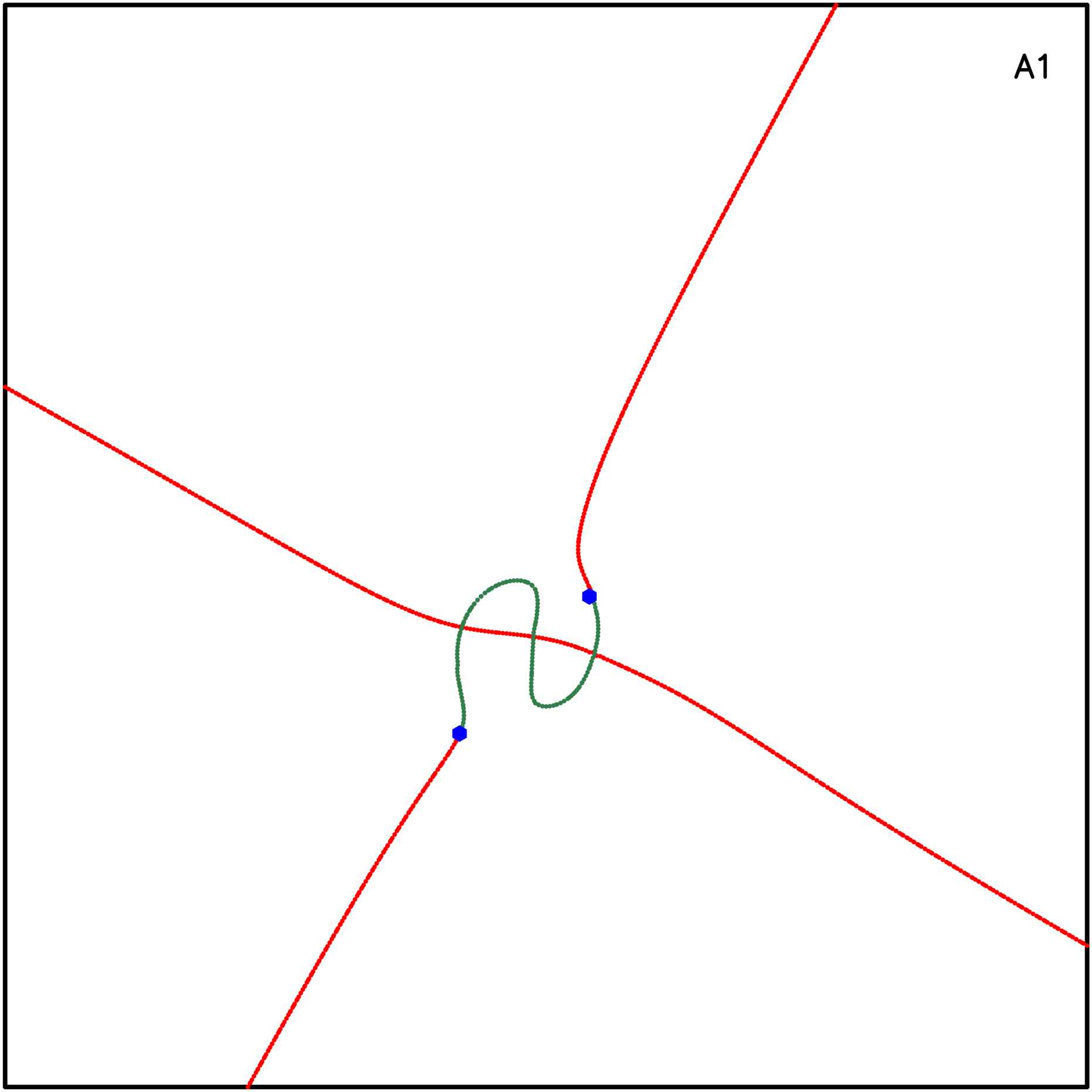
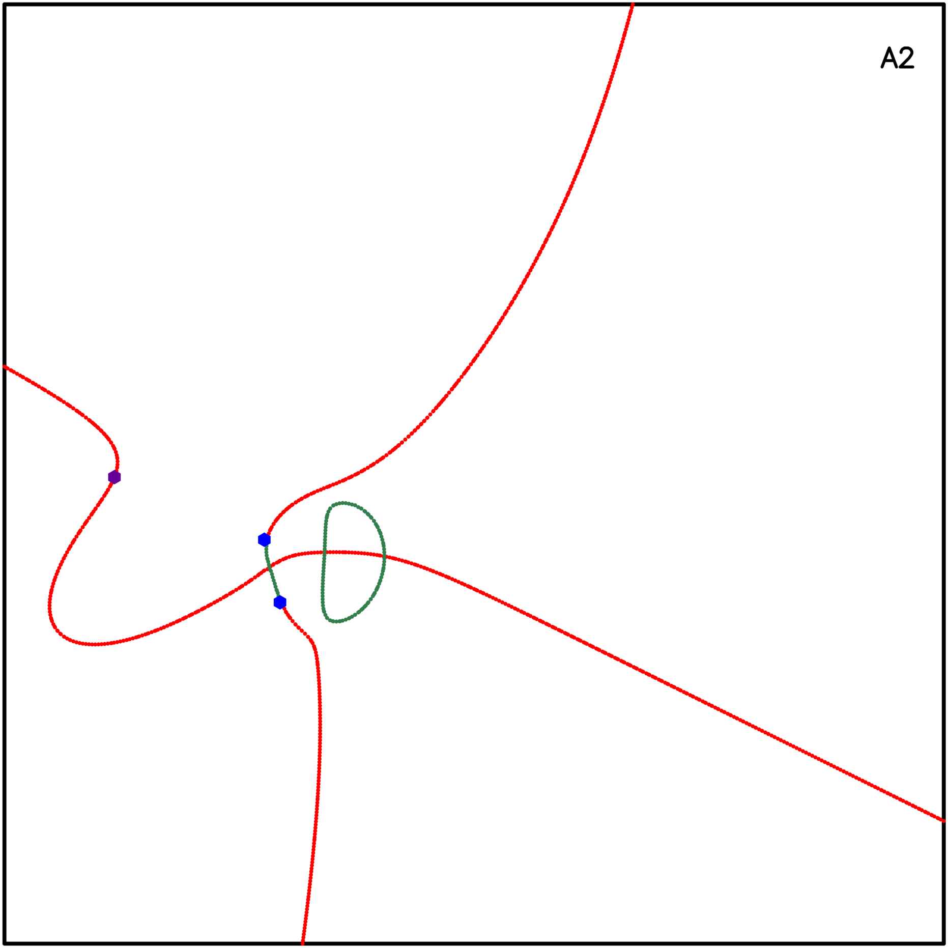
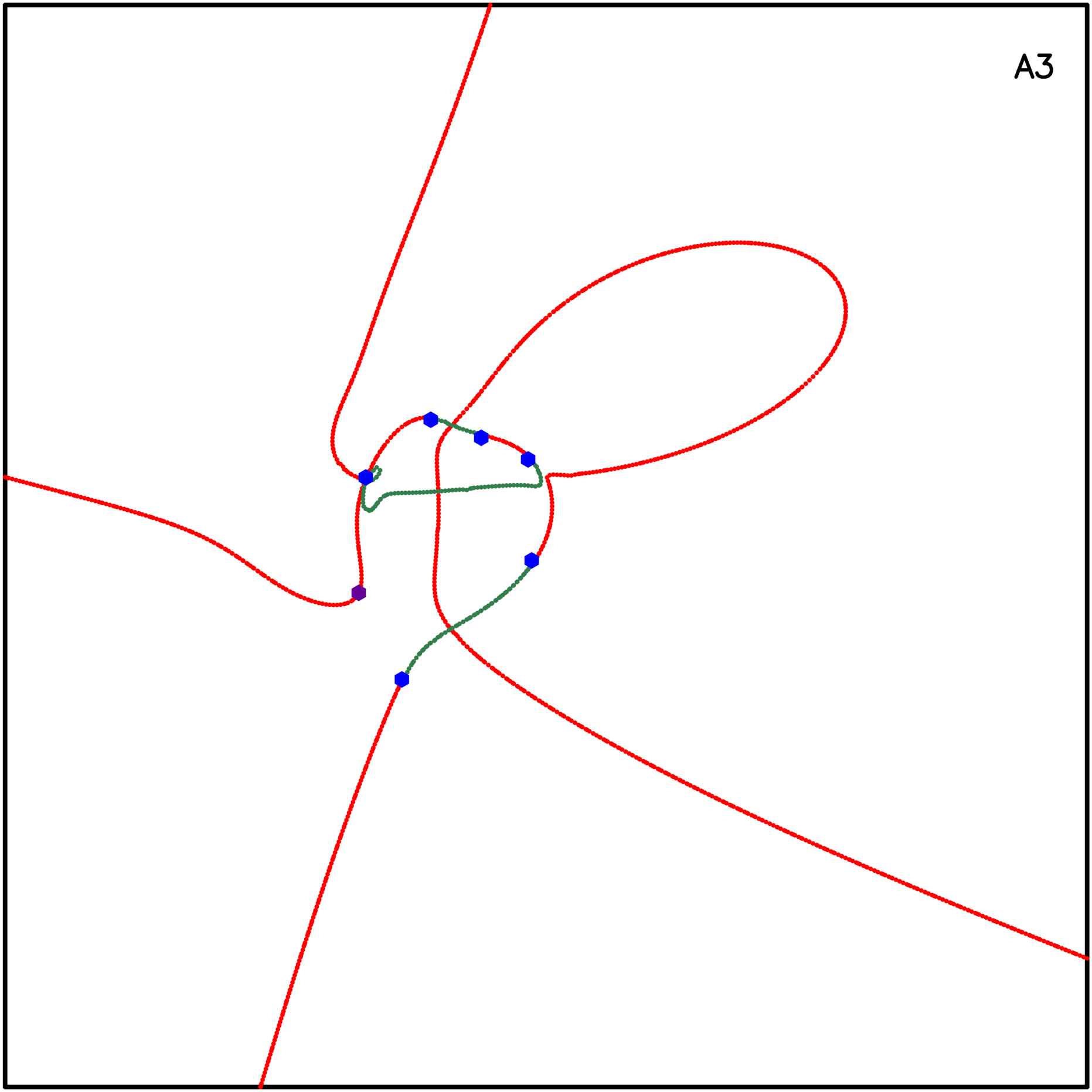
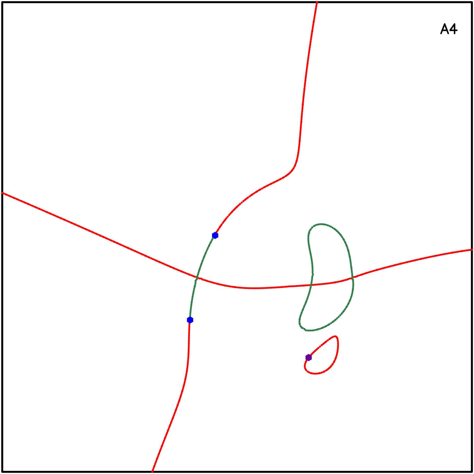
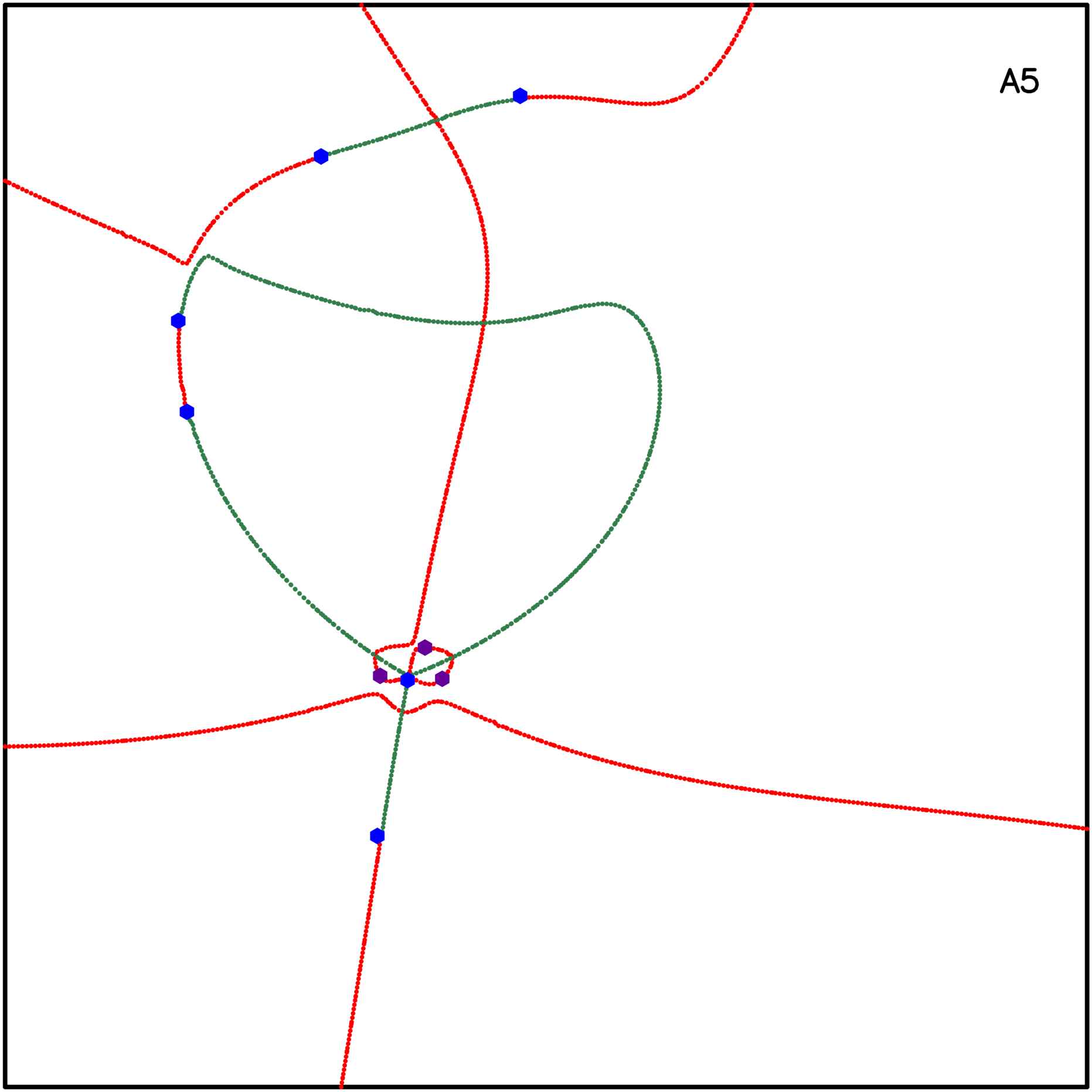
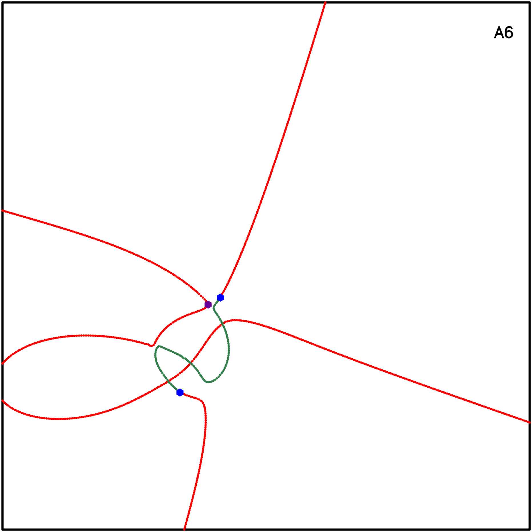
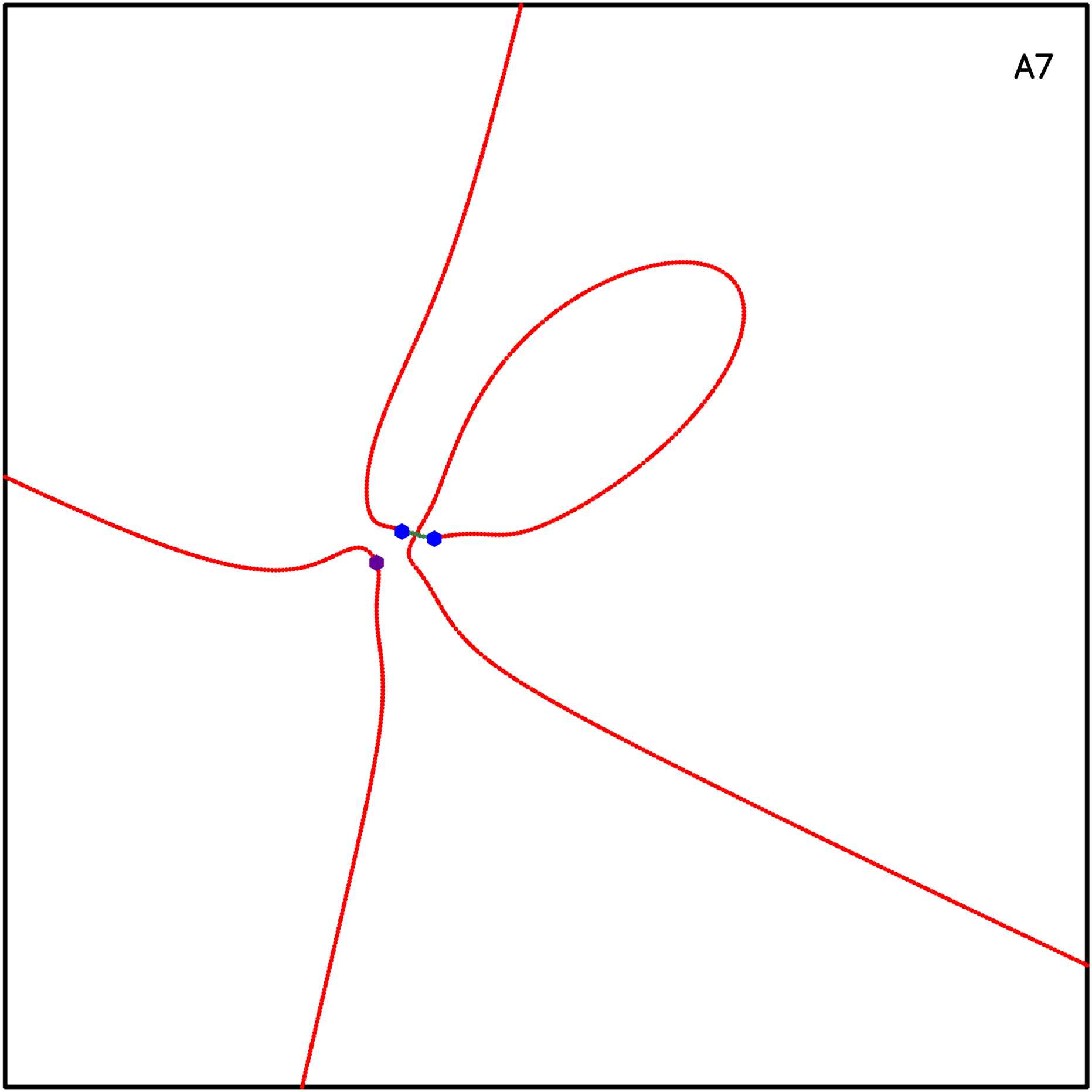
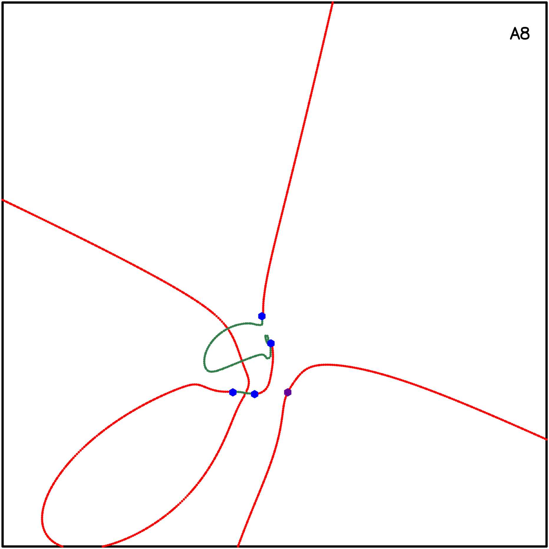
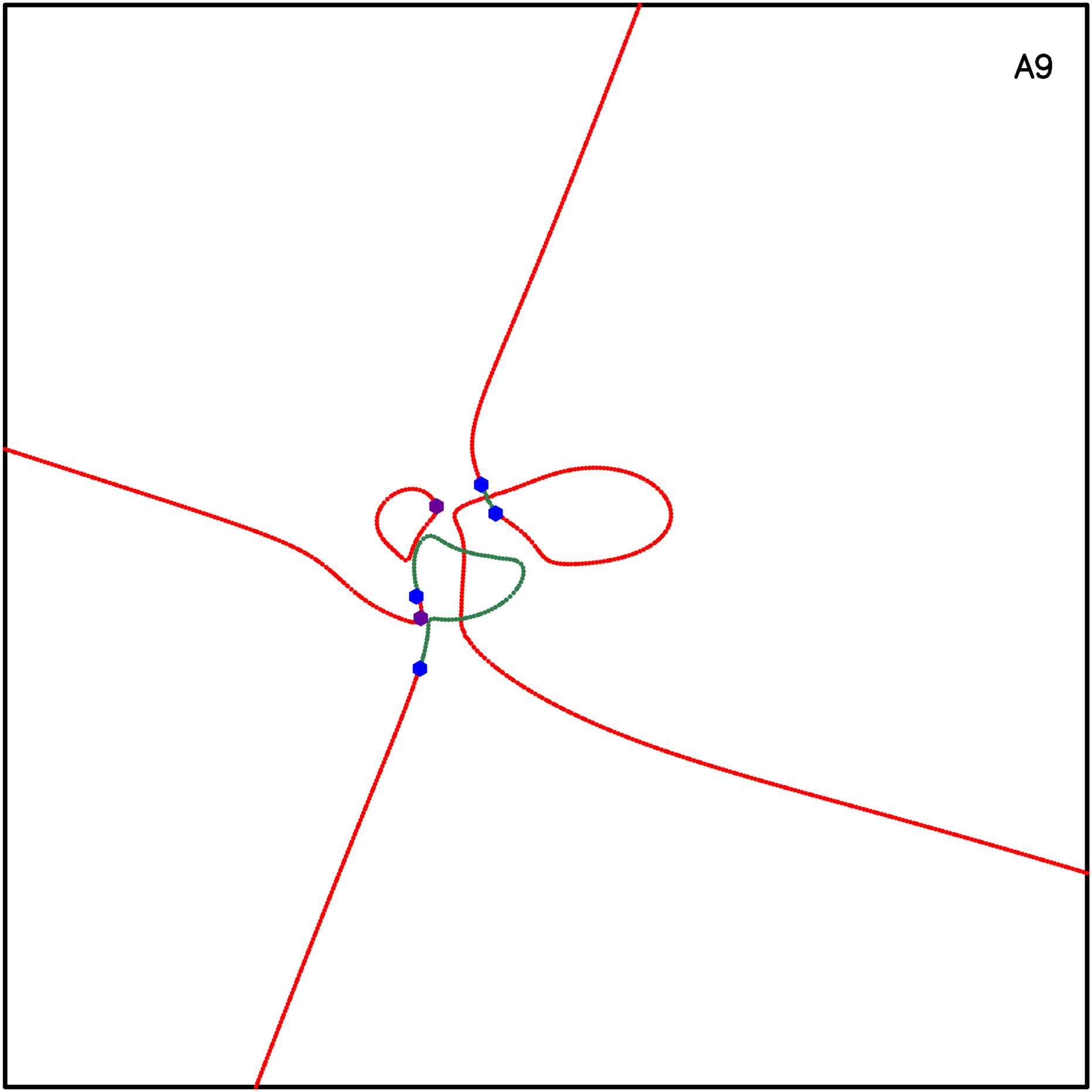
Figure 4: Singularity maps for different positions and orientations of the secondary lens in case of two-component elliptical lens with a fixed position and orientation of primary lens. The red and dark green lines are the $A_{3}$-lines with swallowtail and umbilics denoted by violet and blue points, respectively. The position and number of unstable singularities change with the change in lens parameters. Which shows the strong dependency of singularity map on the lens parameters.

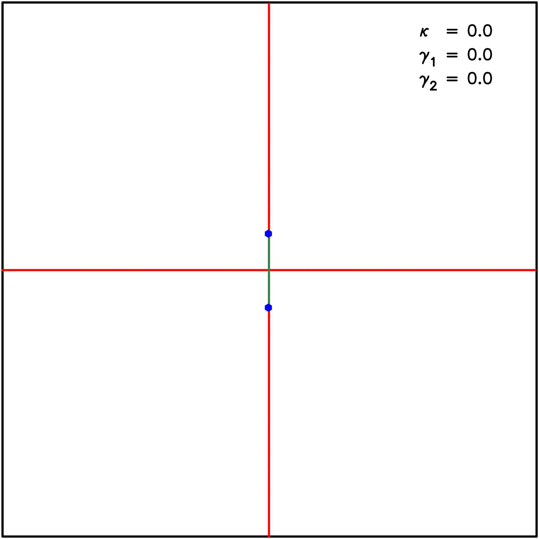
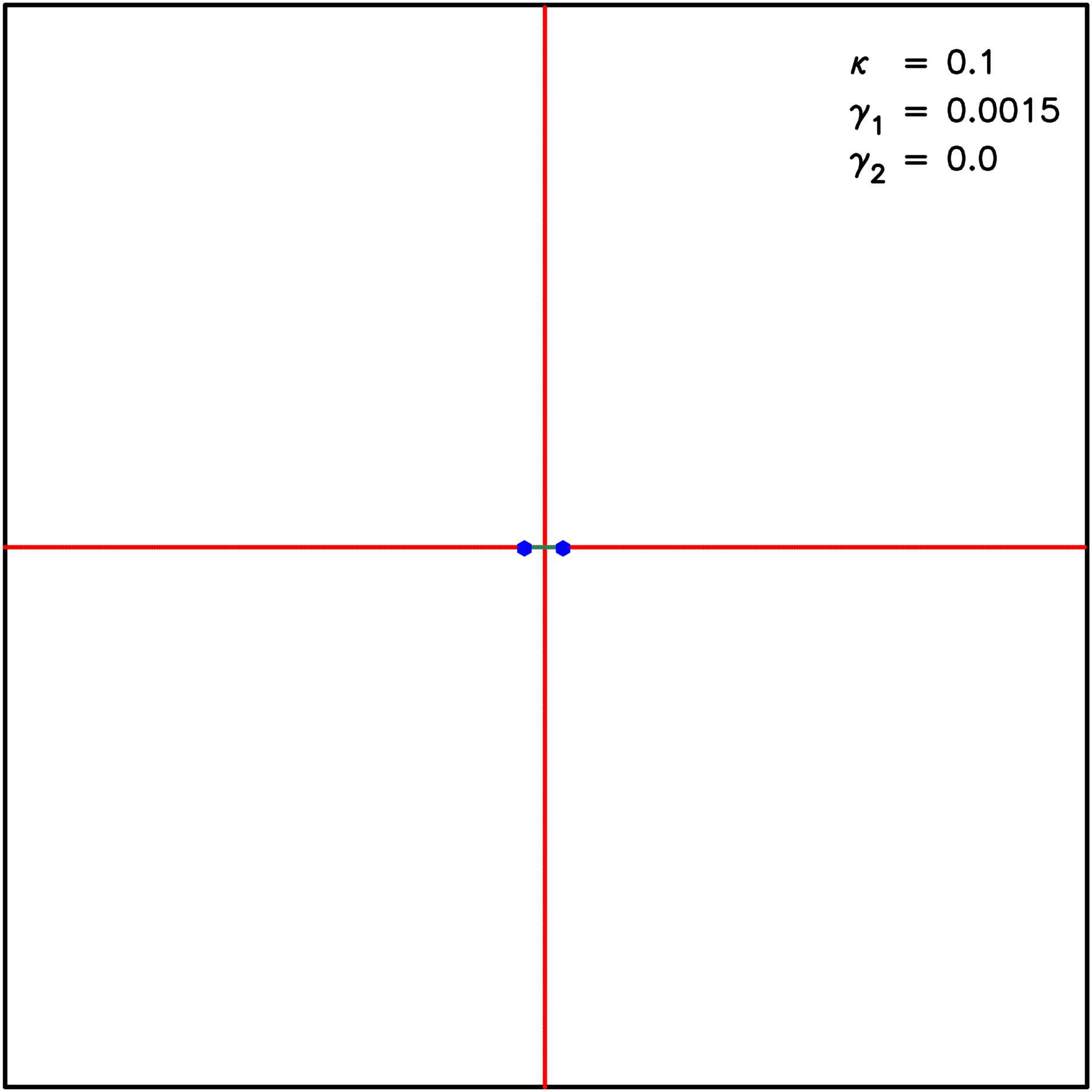
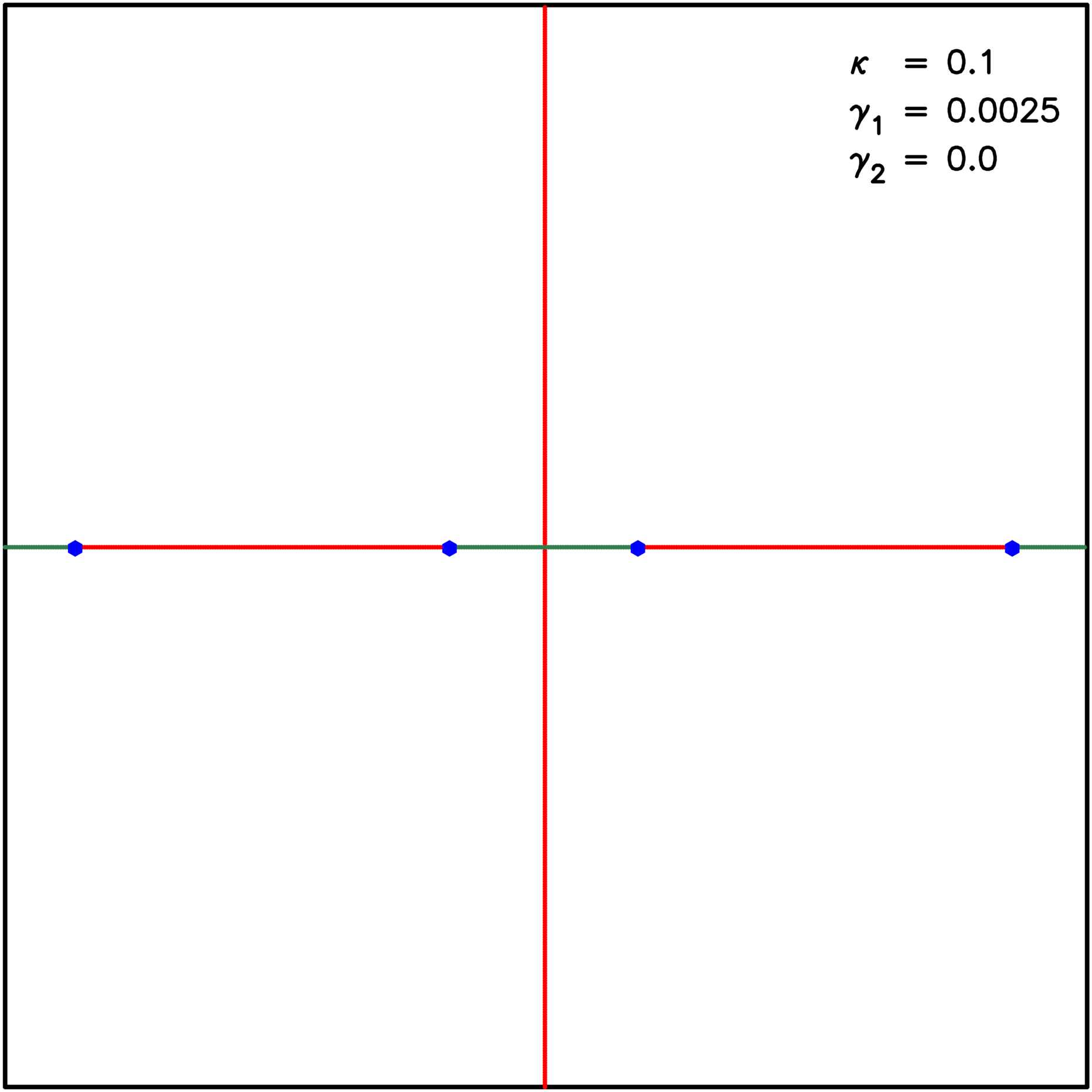
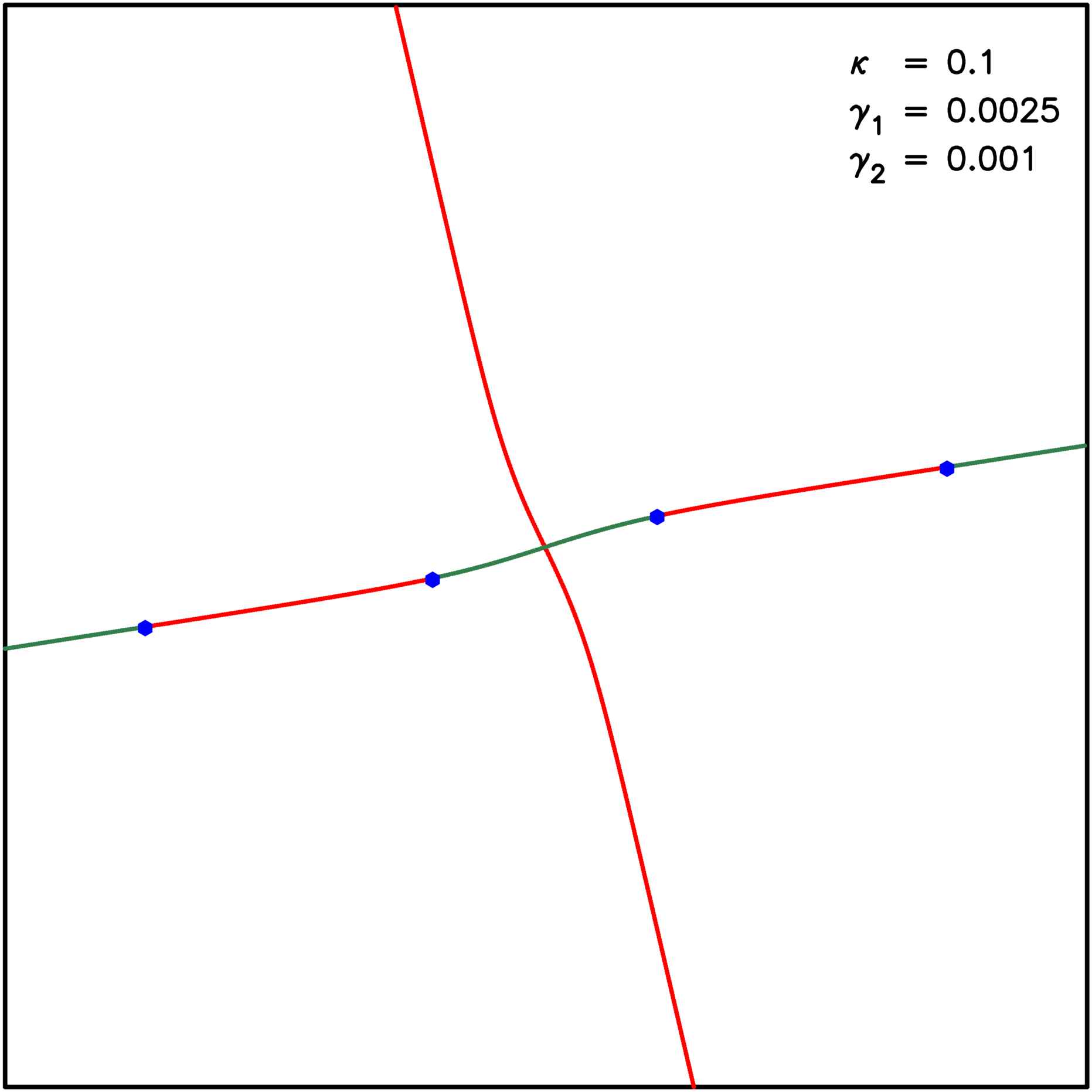
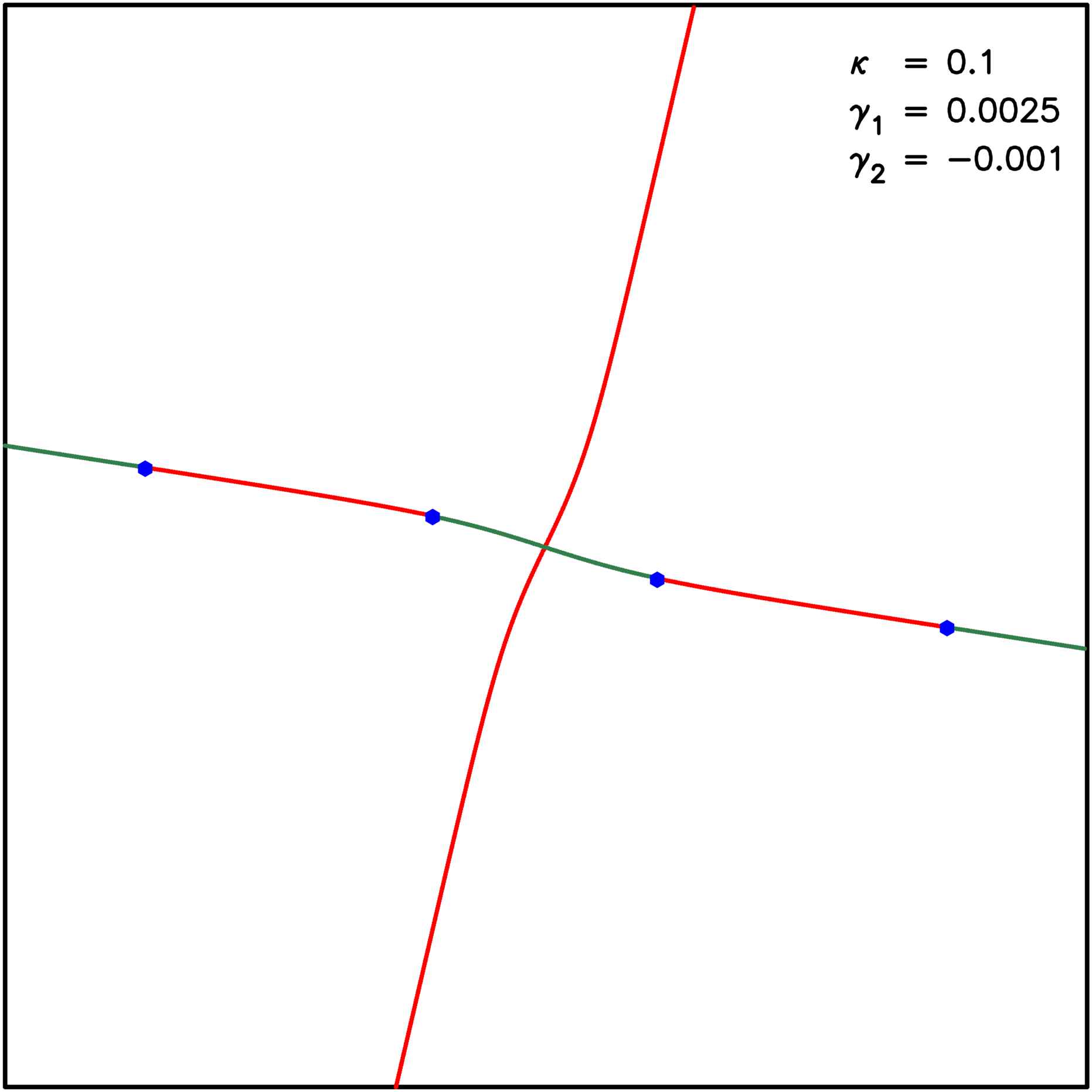
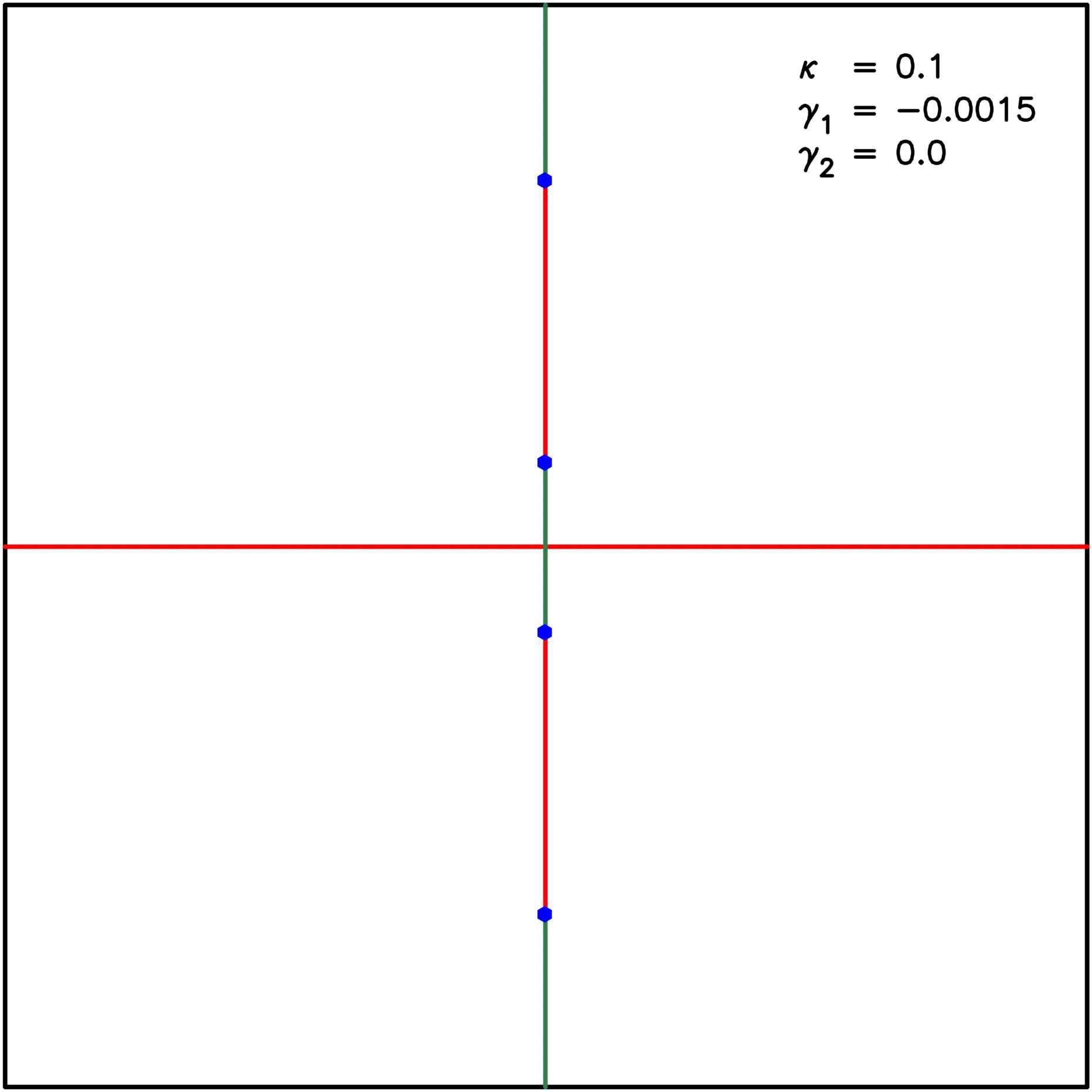
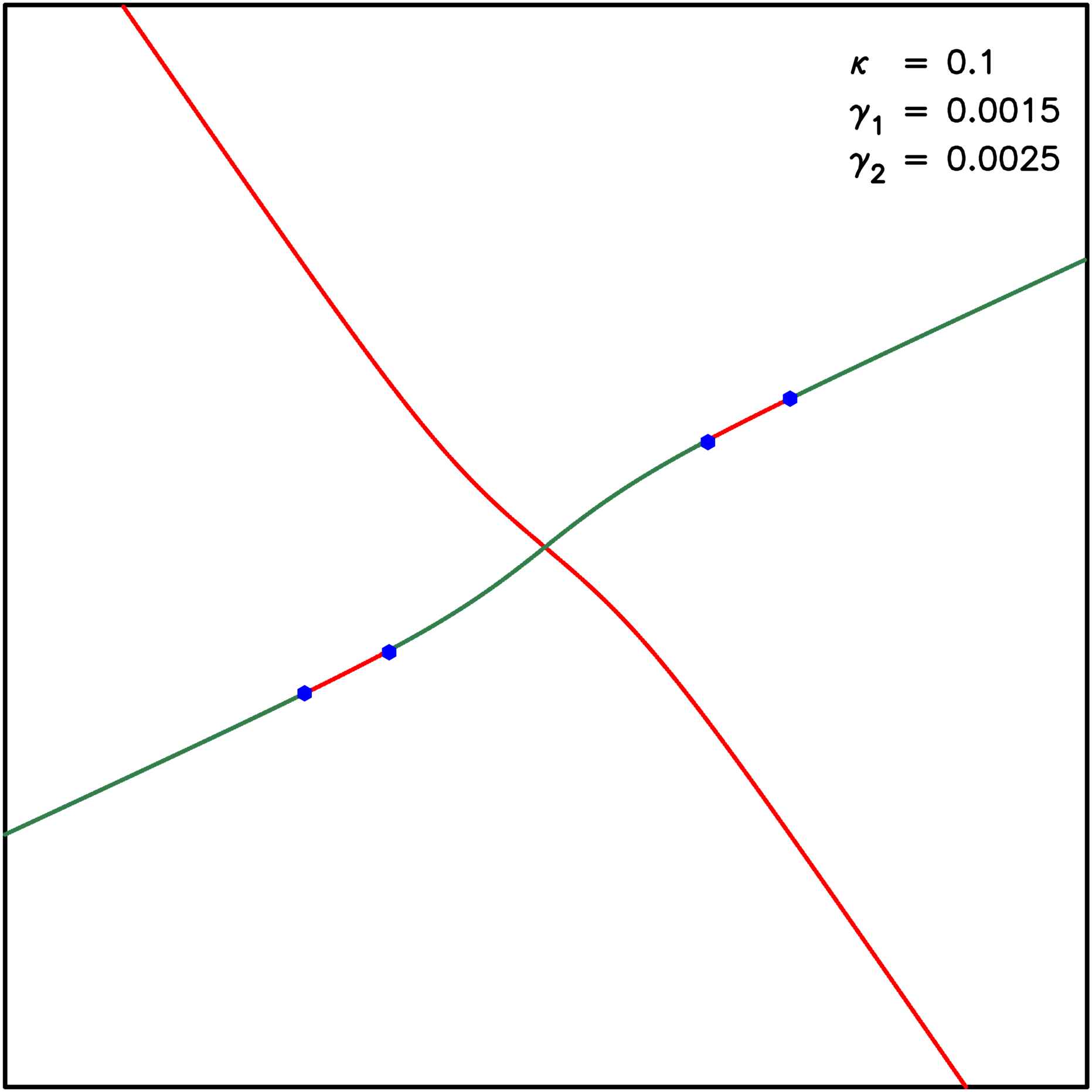
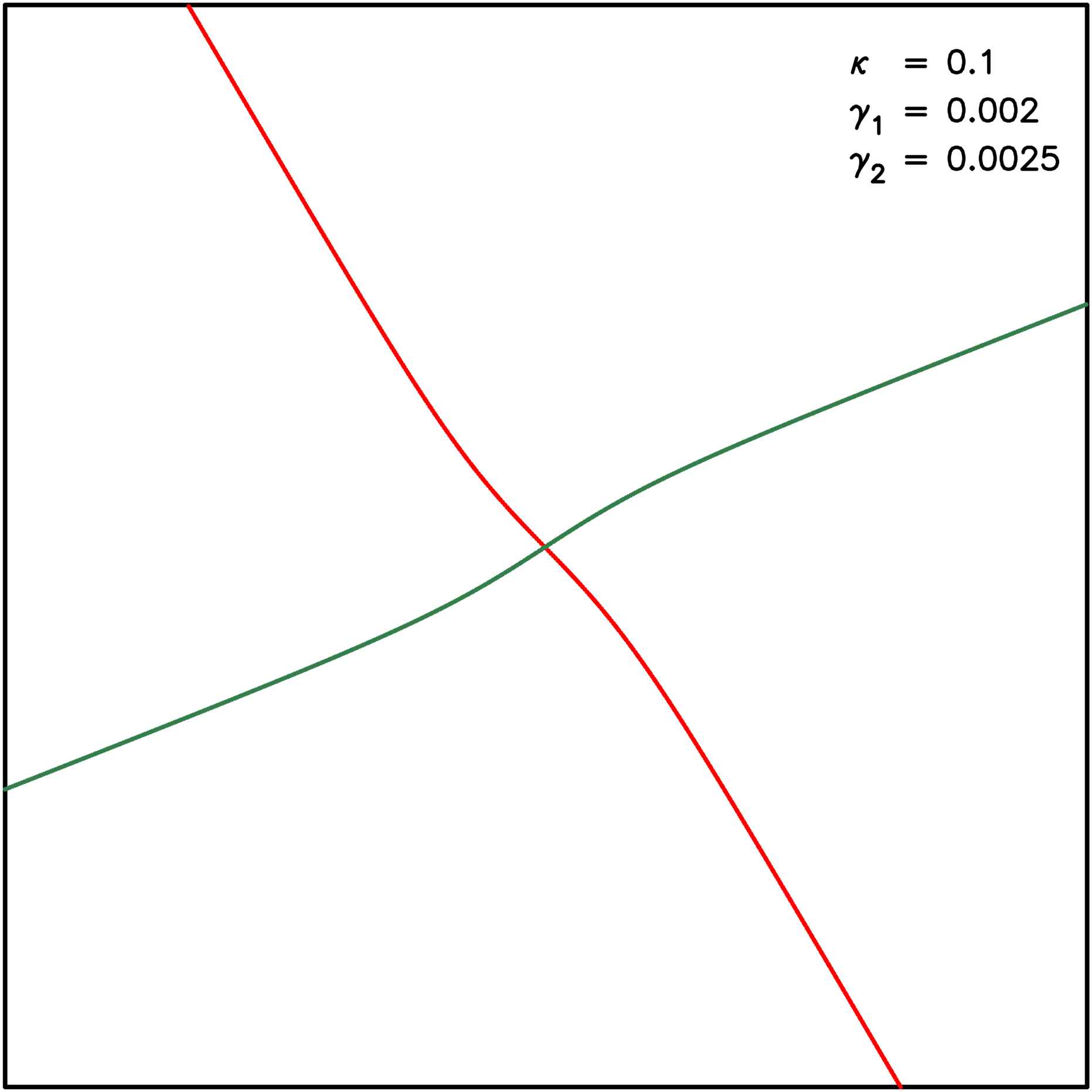
Figure 5: Effect of external convergence and shear on singularity map in case of a one-component elliptical lens. One can see the motion of extra pair of umbilics towards the already existing pair of umbilics. After a certain amount of external shear all point singularities disappear from the singularity map (bottom-right panel).

3 Classification of Singularities

In this section we discuss classification of singularities presented in the lens mapping. The singularities refer to situations where the map from the image plane to the source plane is no longer one to one, and an infinitesimal solid angle in the image plane maps to zero solid angle in the source plane. There are two stable singularities: fold and cusp, and these are present in all situations when we have formation of multiple images. Thus, in general, a caustic in source plane represents cusps connected by folds. The corresponding curve in the image plane is called the critical curve and is expected to be smooth. In the following discussion, we will encounter other singularities, e.g., beak-to-beak, swallowtail, elliptic and hyperbolic umbilics, but these are not stable. These occur only for specific source redshifts with specific lens parameters Schneider et. al. (1992); Bagla (2001). At these unstable singularities, cusps are either created or destroyed or there is an exchange of cusp between radial and tangential caustics in such a way that the total number of the cusps in source plane always remains even. All these unstable singularities are point singularities and have characteristic image formations.

The classification of all these singularities is based on catastrophe theory. In the context of lensing, catastrophe theory describes the singularities in terms of derivatives of the Fermat potential, $\phi(\mathbf{x},\mathbf{y})$ (e.g. SEF, Petters et. al. (2001)), which is related to the lensing potential $\psi(\mathbf{x})$ as,

$$\phi(\mathbf{x},\mathbf{y})=Const.\left(\frac{1}{2}\left(\mathbf{x}-\mathbf{y}\right)^{2}-\psi(\mathbf{x})\right).$$ (9)

Instead of using Fermat potential one can also use deformation tensor (which is completely determined by its eigenvalues and eigenvectors) to discuss different singularities that occur in gravitational lensing. In this way, one does not have to worry about the source parameters, which affect the Fermat potential. The benefit of using deformation tensor instead of Fermat potential is that one does not have to draw critical lines and caustics for all possible source redshift in order to find highly magnified regions in the image plane. And the study of deformation tensor gives a singularity map (in the lens plane) of all possible singularities that can occur for a given lens model for all source redshifts. In our analysis we do not focus on the source redshift but list all the singularities of the map. This approach enables us to focus on these singularities and attempt statistical analysis in typical lens models. This also brings in its own limitations: we are unable to discuss folds as these have an explicit source redshift dependence. This however can be recovered without much work after the singularities have been mapped.

3.1 $A_{3}$-lines

$A_{3}$-lines are the essential elements of the singularity map for a given lens model. In the image plane, these are the lines on which cusps form. As all point singularities are associated with creation, destruction or exchange of cusps, our first goal is to identify the $A_{3}$-lines for a lensing potential.

In the image plane $A_{3}$-lines pass through the points where the gradient of the eigenvalue of the deformation tensor is orthogonal to the corresponding eigenvector $n_{\lambda}$,

$$n_{\lambda}.\nabla_{x}\lambda=0.$$ (10)

Which implies that at $A_{3}$-lines the eigenvector $n_{\lambda}$ is tangent to the corresponding eigenvalue contour (Arnold et. al., 1982; Hidding et. al., 2014). The reader may note that this is also true at points where the eigenvalues have extrema, however such points are isolated. At generic points along these lines an infinitesimal portion of the critical curve, which essentially is a contour level for the eigenvalue, is mapped onto itself as we go from the image plane to the source plane.

In case of a spherically symmetric lens, every point in the lens plane satisfies equation (10). As a result, a spherical symmetric lens gives a formation of point caustic in source plane (SEF) at any point.

In general, we observe two different sets of $A_{3}$-lines in lens plane, one for each eigenvalue of the deformation tensor. The points in the lens plane where $A_{3}$-lines and the corresponding eigenvalue contour (with $\alpha$ or $\beta=1/a$) cross each other correspond to the cusp singularities in source plane at that redshift.

These lines do not intersect each other though as we shall see, lines corresponding to the two eigenvalues can meet at degenerate points ($\alpha=\beta$). The presence of $A_{3}$-lines itself proves the stability of cusp singularities in lens mapping: changing the redshift of the source plane merely shifts the cusp to a neighbouring point.

3.2 Swallowtail Singularities

In the image/lens plane, swallowtail singularities mark the points where eigenvector $n_{\lambda}$ of deformation tensor is tangent to the corresponding $A_{3}$-line. Which implies that at a swallowtail singularity the corresponding eigenvalue ${\lambda}$ reaches a local maxima along $A_{3}$-lines, but this is not a true local maxima (Arnold et. al., 1982; Hidding et. al., 2014). We use this method to identify swallowtail singularity in lens maps.

The characteristic image formation for a swallowtail singularity is an elongated arc. This arc is made up of four images. As we move away from swallowtail singularity the arc changes into distinct multiple images. At a swallowtail singularity, the number of cusps in source plane change by two: a section of fold bifurcates into two cusps at this point.

Figure (1) illustrates the caustics and critical curves in source and lens plane around a redshift at which a swallowtail singularity becomes critical. The lens model used here is a two-component softened elliptical isothermal lens. The first column shows the formation of tangential (radial) caustics, denoted by thick (thin) lines, in the source plane for three different redshifts including redshift $z_{s}$, at which the swallowtail singularity becomes critical (panel B1). The second column shows the corresponding critical curves and the singularity map consisting of $A_{3}$-lines (red for $\alpha$ and dark green for $\beta$ eigenvalue) and other singularities in the lens plane. Position of the swallowtail singularity is denoted by a violet point on the $A_{3}$-line: this is the point where the $A_{3}$ line is tangential to the critical curve. The blue points denote the position of hyperbolic umbilics, discussed in the following subsection. The third column shows the corresponding image formation in lens plane for a given source position in source plane. To see the multiple image formation, we take a circular source: a different color in each quadrant. Such a multi-color source is helpful to recognize positive and negative parity images. The source is shown in the source plane in panels in the left column. A circle is plotted around the source for easy localisation, this circle is not used in the lensing map. The top-left panel (A1) shows the caustics for a redshift smaller than the $z_{s}$ with a circular source lying outside to both caustics. In the lens plane (top-right panel (A3)), we observe a single distorted image. As the source redshift is set to $z_{s}$ (panel (B1)), we can see a kink (origin of two extra cusps) in the tangential caustic near the source position. In panel (B1), the centre of the source in source plane lies on this kink. In the corresponding lens plane (B2) at swallowtail singularity three vectors: tangent to the $A_{3}$-line, tangent to the eigenvalue contour and the local eigenvector are parallel to each other. As we can see in panel (B2), an $A_{3}$ line coming in from outside the critical curve just touches the critical curve at the $A_{4}$ point and falls back to the outer region. The corresponding image formation (B3) shows formation of a tangential arc made of four images. The magnification factor ($|\mu\left(r\right)|$) around a swallowtail singularity is proportional to $r^{-3/4}$, where $r$ is the distance from the singular point. Whereas in the case of fold (cusp), the magnification factor proportional to the $r^{-1/2}$ ($r^{-2/3}$). Hence, the slope of the magnification factor around the swallowtail singularities is steeper than fold and cusp (Arnold et. al., 1982).

As we further increase the source redshift (C1) newly formed cusps in source plane move away from each other and the corresponding arc in lens plane (C3) become more stretched. One can see that the arc in the lens plane is made of four images, two of them have positive parity and two of them have negative parity. Due to the finite size of the source, the images shown here are merging into one another. And the image on the upper left corner has positive parity. Eventually, the gradual increment in the source redshift changes the arc into four individual images. Formation of such giant arcs around swallowtail singularities has been already encountered in investigations of strong lens systems, see, e.g., Saha et. al. (1998); Suyu & Halkola (2010).

3.3 Umbilics

For a given lens model, the presence of umbilics in the corresponding singularity map denote the points with zero shear $\left(\gamma\right)$ in lens plane. At these points, both of the eigenvalues of the deformation tensor are equal to each other ($\alpha=\beta$). The dependence on both eigenvalues simultaneously separates these singularities from the $A_{3}$-lines and swallowtail singularities, which have dependency on one eigenvalue in their definitions. The equality of both eigenvalues implies that at umbilics, eigenvectors of the deformation tensor are degenerate. As a result, any vector at these points can behave as an eigenvector. We can always choose the eigenvector in such a way that $A_{3}$-line condition is always satisfied (for a quantitative analysis see Hidding et. al. (2014)). At these points $A_{3}$-lines corresponding to different eigenvalues meet with each other. There are two types of umbilics present in gravitational lens mapping: elliptic and hyperbolic umbilics. This division of the umbilics depends on the sign of the quantity $s_{D}$,

$$\begin{split}s_{D}\equiv t_{111}^{2}t_{222}^{2}-3t_{112}^{2}t_{122}^{2}-6t_{111}t_{112}t_{122}t_{222}\\ +4t_{111}t_{122}^{3}+4t_{222}t_{112}^{3}\,\,,\end{split}$$ (11)

where $t_{ijk}=\frac{\partial\psi_{ij}}{\partial x_{k}}$. If $s_{D}$ is positive, the singularity is called hyperbolic umbilic and if it is negative then the singularity is an elliptic umbilic. At umbilics, the number of cusps in the source plane remains unchanged but there is an exchange of one or three cusps between tangential and radial caustics depending on the type of the umbilic. In case of a hyperbolic umbilic, one cusp is exchanged between the tangential and the radial caustic: in the image plane an $A_{3}$-line corresponding to each of the two eigenvalues meet at this point. Whereas three $A_{3}$-lines of each of the two eigenvalues meet at the elliptic umbilic in the image plane, and three cusps are exchanged between the tangential and the radial caustic in the source plane.

In order to discuss the evolution of the caustics and critical curves near a hyperbolic umbilic (because of the simplicity of its singularity map) we use a one-component elliptical lens. The evolution of caustics and critical curves near a hyperbolic umbilic is shown in figure 2. The $A_{3}$-lines in the singularity map (middle column) are denoted by red and dark green lines for two different eigenvalues. The positions of hyperbolic umbilic in lens plane is denoted by blue points, at which two $A_{3}$-lines (one for $\alpha$ and one for $\beta$ eigenvalue) meet with each other. For a redshift smaller than the redshift at which hyperbolic umbilic becomes critical, $z_{u}$ both (radial and tangential) caustics in source plane each have two cusps (A1). As we increase the source redshift to $z_{u}$, there is an exchange of cusp from radial caustic to tangential caustic (panel B1) (For the single component elliptical lens model, because of the symmetry of the lens model, both of the hyperbolic umbilics become critical at the same redshift. The symmetry is broken in presence of a second component or shear.). The corresponding image formation (panel B3) shows a single demagnified image with positive parity and a loop formed by four images, two of them with positive parity and two of them with negative parity. As we increase the source redshift further, source plane has a diamond shaped tangential caustic and a smooth radial caustic (panel C1) and in lens plane the highly magnified ring shaped image changes into four individual less magnified images (panel C3). The ring and the cross (for higher redshifts) is not centered at the lens centre but is off centre. We have studied the location of the ring by varying the mass profile of the lens and we find that the ring is located where the projected surface density begins to drop sharply. The magnification factor $|\mu|$ falls as $r^{-1}$ around both umbilics as one moves away from the singular point. Thus magnification factor falls much more rapidly around umbilics than other singularities.

The characteristic image formation for the hyperbolic umbilic is a ring or a cross like system centered away from the lens centre. The curvature of the image formation is much stronger and the radius of curvature is much smaller than the size of the lens. So far only one lens system (Abell 1703) with image formation near a hyperbolic umbilic has been seen (Xivry et. al., 2009).

Unlike the hyperbolic umbilic, at an elliptic umbilic, there are six $A_{3}$-lines (three each for each of the two eigenvalues of the deformation tensor) meet with each other. For an illustration, formation of an elliptic umbilic in case of a two-component elliptical lens model is shown in the figure (3). We find that often, two of three $A_{3}$-lines of one or both eigenvalues form a small closed loop. This can be seen in examples shown in figure 4. In panel (A1), we only see tangential caustics, and the source lies inside the triangular shaped caustic. Panel (A3) shows the characteristic image formation (seven images in a shape of Y) near an elliptic umbilic. The central image has positive parity. The next three images from the central image have negative parity. And the three outer images again have positive parity. As we increase the source redshift, the size of the triangular shaped caustic decreases and at the same time, it moves away from the source position. At a redshift $z_{p}$, where the elliptic umbilic become critical it become a points caustic (panel B1) and the source lies close to this point caustic. The corresponding images still form a Y-shaped structure in lens plane but with only five images. As we further increase the source redshift, the point caustic turns into a triangular shaped radial caustic (panel C3). Which implies that at the elliptic umbilic there is an exchange of three cusps between tangential and radial caustic. In panel (C1), we moved the source inside the triangular caustic, to see whether it still gives a Y-shaped image formation. We get a different kind of image formation with central image rotated by $\pi/2$.

Figure 3, shows the singularity map close to the elliptic umbilic (shown by blue point). Swallowtail singularities are shown as violet points. The complete singularity map for figure 3 is given in figure 4 (panel A5).

The characteristic image form is six images radiating out from the singularity. The singularity need not coincide with the centre of the lens, The images do not have any tangential deformation.

4 Algorithm

We briefly discuss the algorithm used to find out the singularities for a given lens model, we focus on singularities that are discussed in above section. We set up a uniform grid in the lens plane for calculations of physical quantities in order to locate the singularities. The grid-size depends on the resolution required for the lens model, in general we require adequate resolution as we are dealing with non-linear combinations of second derivatives of the lensing potential, even the smallest features should be well resolved on the grid. We use finite difference methods to compute derivatives on the grid. To calculate the position of the umbilics in the lens plane, we use the fact that at umbilics, both components of the shear tensor vanish, identically. Our approach closely follows that of Hidding et. al. (2014). The flow of the code is as follows:

• INPUT (Lens Potential)

• CALCULATE first and second derivatives of the potential

• CALCULATE eigenvalue and eigenvectors of the deformation tensor

• CALCULATE gradient of eigenvalue

• CALUCLATE extrema

  • CALCULATE local maxima

  • CALCULATE local minima

• Identify points on $A_{3}$-lines using Equation 10.

• Identify $A_{4}$-points using the algorithm given in §3.2

• Identify $D_{4}$-points using the algorithm given in §3.3

The potential of the given lens model is the input in this algorithm. The potential can be computed from a mass model, or be provided directly. Given the potential, the deformation tensor is computed at each point followed by calculation of its eigenvalues and corresponding eigenvectors. This information along with gradient of eigenvalues is sufficient to identify points on the $A_{3}$-lines (eq. (10)). Note that points on the $A_{3}$-lines can be identified on the mesh and need not coincide with the grid points. The points need to be ordered to construct curves: this is required for identifying $A_{4}$ points as we need to locate maxima of eigenvalue along the $A_{3}$-lines. By rejecting such extrema that are also local maxima, we are left with $A_{4}$ points.

We find that it is simpler to identify umbilics by realizing that the diagonal components of the deformation tensor are equal, and the off-diagonal component of the deformation tensor (shear) vanishes. Each of these conditions specifies curves in the image plane, and intersections of these curves give us umbilics. We can classify the type of umbilics by counting the number of $A_{3}$-lines that converge at this point.

5 Results

We apply our algorithm by applying it to a single component lens where the potential can be expressed in a closed form and the image structure has been studied in detail. Then we apply it to multi-component lenses and study a variety of configurations. Lastly we apply it to one real lens model. As mentioned above in subsection 3.1, this technique does not work in case of isolated spherically symmetric lenses because of the absence of cusp formation. We study elliptical lenses with one and two components. In the case of one-component elliptical lens, there are two $A_{3}$-lines and two hyperbolic umbilics. Whereas for two-component lens, the location of $A_{3}$-lines and other singularities in lens plane depend on the lens configuration.

We also discuss the behaviour of swallowtail and umbilics in a lens model under external perturbations in case of one and two component elliptical lenses. This gives us the estimate about the amount of external shear under which a singularity does not vanish from the lens plane and hence gives us an idea about how robust these point singularities really are. In the following subsections, we will discuss the singularity maps for elliptical lenses and Abell 697 in detail. After that we study the stability of these different singularities in lens mapping.

Figure 6: Image formation and singularity map for Abell 697: The left panel shows caustics, the middle column shows critical curves in the image plane and the right column shows the lensed images. The top panel represent image formation near a swallowtail singularity at source redshift $z_{s}=0.67$. The two middle panels represent image formation for a source at $z_{s}=0.82$ and the bottom panel represent image formation for a source at redshift $z_{s}=2.0$.

5.1 One-Component Elliptical Lens

We first consider a one component elliptical lens. This is a good model for an isolated lens that is dynamically relaxed, e.g., an isolated galaxy or a cluster of galaxies. The elliptical isothermal lens with a finite core has a potential of the form:

$$\psi(x_{1},x_{2})=\psi_{0}\sqrt{r_{0}^{2}+\left(1-\epsilon\right)\left(x_{1}-x_{01}\right)^{2}+\left(1+\epsilon\right)\left(x_{2}-x_{02}\right)^{2}},$$ (12)

where $r_{0}$ is the core radius of the lens, $\epsilon$ is the ellipticity, $\left(x_{01},x_{02}\right)$ are the coordinates of the centre of the lens with respect to the optical axis and $\psi_{0}$ describes the strength of the lens.

The characteristics of this lens are described in detail in Blandford $\&$ Narayan (1986) (See Figure 10). The singularity map in lens plane for this lens model is shown in figure (2) (middle column (A2,B2,C2)). It has two $A_{3}$-lines (represented in red and dark green) for two eigenvalues of the deformation tensor, running along the major and the minor axis of the lens potential. This lens model also has two hyperbolic umbilics along the minor axis and their position depends on the lens parameters, primarily on the core radius $r_{0}$. Because of the elliptical symmetry in the lens model, both umbilics lie at the same distance from the centre of the lens. As a result, both umbilics become critical at the same source redshift. If we change the core radius, this distance from the centre and the redshift at which these hyperbolic umbilics becomes critical, also change.

5.2 Two-Component Elliptical Lens

Most realistic lenses have several components, though one of the components may dominate over others. In this section we consider two component lenses. We consider one primary (dominant) and one secondary component. Presence of the secondary component significantly affects lensing due to primary lens. In order to include the effects of the secondary lens, one has to modify the lensing potential in equation (8). If the secondary lens also an elliptical lens (for simplicity), then the lens potential becomes:

$$\psi(x_{1},x_{2})=\psi_{p}+\psi_{s},$$ (13)

with $\psi_{p}$ and $\psi_{s}$ are one component elliptical lenses centered at different points in the image plane with different core radii and ellipticities and the major axes of the two components can be at an angle. ($r_{01}\,\left(r_{02}\right)$ are the corresponding core radii for the two potentials, $\epsilon_{1}\,\left(\epsilon_{2}\right)$ is the ellipticity and $\left(x_{11},x_{12}\right)\,\left(\left(x_{21},x_{22}\right)\right)$ are the coordinates of the centre of the primary (secondary) lens with respect to the optical axis.)

Different sets of lens parameters give different kinds of singularity map and image formation. For example, figure (1) and figure (3) represent singularity map for two-component lens models with two different set of lens parameters. Figure (4) shows some other possible singularity maps for two-component elliptical lens with a fixed primary lens and different (randomly picked) position and orientation of the secondary lens. As before, red and dark green lines represent the $A_{3}$-lines with swallowtail and umbilic points denoted by violet and blue points, respectively. One can see the dependency of unstable singularities on lens parameters: as we change the secondary lens the position and critical redshift for the unstable singularities also changes. From figure (4), we also gain some knowledge about the sensitivity of the unstable singularities to the lens parameters. All panels in figure (4) have hyperbolic umbilics and swallowtail (except first panel), whereas only three panels show elliptic umbilics. We infer that elliptic umbilics are more sensitive to the lens parameters than the swallowtail and the hyperbolic umbilic.

5.3 Stability

In general, finding an isolated gravitational lens with one or two components is highly unlikely. Real gravitational lenses reside in an environment made of several structures. These external local structure perturb the lensing potential, by introducing (constant) external convergence ($\kappa_{ext}$) and shear ($\gamma_{ext}$). As a result, the perturbed lensing potential is given by,

$$\psi(x_{1},x_{2})=\psi_{p}+\frac{\kappa_{ext}}{2}\left(x_{1}^{2}+x_{2}^{2}\right)+\frac{\gamma_{1}^{\prime}}{2}\left(x_{1}^{2}-x_{2}^{2}\right)+\gamma_{2}^{\prime}x_{1}x_{2},$$ (14)

where $\psi_{p}$ is the potential of primary lens, given by equation (12) or (13) in case of elliptical lenses or given by some other profile and $\left(\gamma_{1}^{\prime},\gamma_{2}^{\prime}\right)$ denotes the component of external shear ($\gamma_{ext}$).

The effect of the external convergence ($\kappa_{ext}$) is equivalent to the addition of a constant mass sheet in the lens model, which simply changes the total strength of the primary lens. As a result, the critical redshift for unstable singularities changes, but neither the unstable singularities vanish nor the location of $A_{3}$-lines in lens plane changes due to the presence of external convergence. On the other hand, the presence of external shear ($\gamma_{ext}$) shifts the location of $A_{3}$-lines significantly and as a result it changes the singularity map for a given lens model. The presence of external shear can also introduce or remove point singularities. The effect of external shear with a fixed value of external convergence in case of a one-component elliptical lens model, (equation (12)) is shown in figure (5). One can see that, for non-zero external shear, two extra hyperbolic umbilics occur in the lens plane along the major or minor axis depending on the values of shear components. As we increase the amount of external shear, this extra pair of umbilics move towards already existing umbilics and merge with them. This implies that introducing a finite amount of external shear can also remove the already existing point singularities from the singularity map and it is possible (in highly symmetric case) to have a singularity map without any point singularities. The amount of external shear $\gamma_{ext}=\left(\sqrt{\gamma_{1}^{\prime 2}+\gamma_{2}^{\prime 2}}\right)$, under which point singularities shift but remain in the lens plane depends on the type of the singularity. In case of hyperbolic umbilic, it is of the order of $10^{-3}$. Similarly, the amount of external shear for which a swallowtail (elliptic umbilic) shifts but survives in the lens plane is of the order of $10^{-4}\left(10^{-5}\right)$. But for some particular directions of external shear, the swallowtail and elliptic umbilics show extra stability, i.e., the magnitude of external shear under which these singularities remain in the lens plane attain a higher value than the other cases. This reinforces the impression from the qualitative study in the last subsection that an elliptic umbilic is less stable as compared to the hyperbolic umbilic and swallowtail.

5.4 Abell 697

After testing our approach with simple model lenses, we apply the algorithm to a real lens to illustrate the utility and efficacy of our approach. We work with the cluster lens Abell 697 $\left(z\,=\,0.282\right)$. We use the data for the lens from RELICS (Cibirka, et al., 2018; Coe, et al., 2019). The reason for choosing the Abell 697 for the preliminary analysis is the relative simplicity of the critical lines in the lens plane. The study of more complicated lenses is under consideration, and the results for a large set of clusters will be presented in a forthcoming paper along with a statistical analysis of occurrence of point singularities. The cosmological parameters used in the calculation of different angular diameter distances are: $H_{0}=70\,kms^{-1}Mpc^{-1}$, $\Omega_{\Lambda}=0.7$, $\Omega_{m}=0.3$. Figure 6 shows the singularity map along with the critical lines and caustics in image and source plane for Abell 697. Here we only considered the central region of Abell 697 with size $440\times 440$pixels (1 pixel =$0.06"$)  (Cibirka, et al., 2018). We can see that the dominant component here is like an elliptical lens and there is a lot of small scale structure contributed by other components in the lens. The role of other components is to increase the length of $A_{3}$-lines and also to introduce point singularities.

The top panel in figure 6 shows the image formation near a swallowtail singularity for a source at redshift $z_{s}=0.67$. The second and third panel shows the image formation for a source at redshift $z_{s}=0.82$ for two different source positions. The bottom panel shows the image formation for a source at redshift $z_{s}=2.0$. Here the source position is chosen in such a way so that it can reproduce the image formation for system 1 in (Cibirka, et al., 2018). One can see that we were able to reproduce the four images for system 1 along with the fifth image, which was not observed due to the contamination from BCG, as mentioned in (Cibirka, et al., 2018). Since we considered a circular source, the shape of the images can be different from (Cibirka, et al., 2018). As one can see from the bottom panel, one pair of hyperbolic umbilic is still outside the critical curves. This means that the critical redshift for this pair is higher than the $1.1$. Locations of these singularities are optimal sites for searching for faint sources at high redshifts.

6 Conclusions

We have analyzed stable and unstable singularities that can occur in strong gravitational lensing. In order to locate these singularities, we have implemented algorithms which take lens potential as an input. We have applied our algorithm in the case of simple lens models as well as a real lens. Singularity map, which comprises all these singularities provides a compact representation of the given lens model in the lens plane. The presence of these unstable singularities in the singularity map can be used to constrain the lens model if we can find a lensed source in the vicinity. Magnification is very large in the vicinity of these singularities and each of these singularities has a characteristic image formation that can be used to identify the singularities. Multiple images in these characteristic image formations lie in a very compact region (of the order of a few arcsec around the singular point) of the lens plane. Further, the regions with $A_{3}$-lines and point singularities are obvious targets for deep surveys that use gravitational lenses to search for very faint sources at high redshifts.

The singularities can be identified using the characteristic image forms. In case of $A_{4}$ points or swallowtail, we get four images in a straight line: the images form an arc with a radius of curvature much larger than the distance from the cluster centre. Abell 370 has an image system of this type. The hyperbolic umbilic (purse) has an image formation of a ring or a cross centered away from the centre of the lens. Further, in this case the radius of curvature of the ring is much smaller than the characteristic radius of the lens system. Such an image system has been seen in Abell 1703 (Xivry et. al., 2009). The elliptic umbillic (pyramid) has images radiating out from a centre, these do not show any tangential distortion. The centre of the image system need not coincide with the centre of the lens system. To the best of our knowledge such an image system has not been seen so far.

We have studied the dependency of unstable singularities on lens parameters as well as on the external shear. The magnitude of external shear under which these singularities remain in the singularity map is different for different singularities. This is of the order of, $10^{-3}$, $10^{-4}$, $10^{-5}$ in case of hyperbolic umbilic, swallowtail and elliptic umbilic, respectively. Thus the elliptic umbilic is most sensitive to perturbations in lensing potential and hence is the most unstable.

The somewhat unstable nature of such singularities can be put to good use in two ways: finding characteristic image formations can be used to constrain lens models, and, with multiple constraints on the lens model we can potentially invert the problem and constrain redshifts of sources to better than what can be achieved with photometric redshifts. These aspects will be investigated and addressed in more detail in a follow up study of known lens systems.

We have applied our approach in case of simple lens models and one real lens: Abell 697. We are studying other lens systems using our approach and an atlas of lens singularities and their statistical analysis will be presented in a forthcoming paper. Such an atlas can be of use for refinement of lens models with further observations and also for targeting specific regions in searches for very faint sources at high redshifts. Along with an atlas of lens models we also propose to construct an atlas of variations around the characteristic image forms. Such an atlas of image forms can be used for training machine learning programs, e.g., see Davies, Serjeant & Bromley (2019). However, for a complete analysis of the lens system, one requires detailed modeling of the gravitational lens.

7 Acknowledgements

AKM would like to thank CSIR for financial support through research fellowship No.524007. This research has made use of NASA’s Astrophysics Data System Bibliographic Services. We acknowledge the HPC@IISERM, used for some of the computations presented here. Authors thank Professor D Narasimha for useful discussions and comments. JSB thanks Professor Varun Sahni and Professor Sergei Shandarin for insightful discussions on singularities and caustics, and also for useful comments on the manuscript. Authors thank Richard Ellis, Prasenjit Saha and Liliya Williams for detailed comments on the manuscript. Authors also thank Ms Soniya Sharma who worked on some aspects of this problem for her MS thesis.

References

- Saha et. al. (1998) Abdelsalam, H. M., Saha, P., Williams, L. L. R. 1998, MNRAS, 294, 734
- Abdelsalam et. al. (1998) AbdelSalam, H. M., Saha P., Williams L. L. R., 1998, AJ, 116, 1541
- Akeson, et al. (2019) Akeson R., et al., 2019, arXiv, arXiv:1902.05569
- Arnold et. al. (1982) Arnold V.I., Shandarin S.F. Zeldovich Y.B., 1982, Geophys. Astrophys. Fluid Dynamics 20, 111
- Atek et al. (2018) Atek H., Richard J., Kneib J.-P., Schaerer D., 2018, MNRAS, 479, 5184
- Bagla (2001) Bagla J. S., 2001, in Brainerd T. G., Kochanek C. S., eds, ASP Conf. Ser. Vol. 237, Gravitational Lensing: Recent Progress and Future Goals. Astron. Soc. Pac., San Francisco, p. 77
- Berry & Upstill (1980) Berry M. V., Upstill C., 1980, PrOpt, 18, 257
- Blandford Narayan (1986) Blandford R. Narayan R., 1986, APJ, 310, 568.
- Blandford et al. (1989) Blandford R. D., Kochanek C. S., Kovner I., Narayan R., 1989, Sci, 245, 824
- Cibirka, et al. (2018) Cibirka N., et al., 2018, ApJ, 863, 145
- Coe, et al. (2013) Coe D., et al., 2013, ApJ, 762, 32
- Coe, et al. (2019) Coe D., et al., 2019, arXiv e-prints, arXiv:1903.02002
- Dark Energy Survey Collaboration, et al. (2016) Dark Energy Survey Collaboration, et al., 2016, MNRAS, 460, 1270
- Davies, Serjeant & Bromley (2019) Davies A., Serjeant S., Bromley J. M., 2019, MNRAS.tmp, 1298
- Ebeling, et al. (2018) Ebeling H., Stockmann M., Richard J., Zabl J., Brammer G., Toft S., Man A., 2018, ApJ, 852, L7
- Gardner, et al. (2006) Gardner J. P., et al., 2006, SSRv, 123, 485
- Gilmore (1981) Gilmore I., 1981, Catastrophe theory for scientists and engineers, Wiley, New York
- Hidding et. al. (2014) Hidding J., Shandarin S. F., van de Weygaert R., 2014, MNRAS, 437, 3442
- Ivezić, et al. (2008) Ivezić Ž., et al., 2008, arXiv e-prints, arXiv:0805.2366
- Kassiola et. al. (1992) Kassiola A., Kovner I. Fort B., 1992, ApJ 400, 41
- Kneib & Natarajan (2011) Kneib J.-P., Natarajan P., 2011, A&ARv, 19, 47
- Laureijs (2009) Laureijs R., 2009, arXiv e-prints, arXiv:0912.0914
- McLeod, et al. (2015) McLeod D. J., McLure R. J., Dunlop J. S., Robertson B. E., Ellis R. S., Targett T. A., 2015, MNRAS, 450, 3032
- Nityananda (1990) Nityananda R., 1990, LNP, 1, LNP…360
- Xivry et. al. (2009) Orban de Xivry, G., Marshall, P. 2009, MNRAS, 399, 2
- Petters et. al. (2001) Petters A. O., Levine H., Wambsganss J., 2001, in Petters A. O., Levine H., Wambsganss J., eds, Progress in Mathematical Physics. Vol. 21. Singularity Theory and Gravitational Lensing. Birkhäuser, Boston
- Poston & Stewart (1978) PostonT., Stewart I., 1978, Catastrophe Theory and its application, Pitman, New York
- Saha et. al. (1997) Saha, P., Williams, L. L. R. 1997, MNRAS, 292, 148
- Saha et. al. (2001) Saha, P. 2000, AJ, 120, 1654
- Schneider et. al. (1992) Schneider P., Ehlers J., Falco E. E., 1992, Gravitational Lenses. Springer- Verlag, Berlin.
- Suyu & Halkola (2010) Suyu S. H., Halkola A., 2010, A&A, 524, A94
- Yuan, et al. (2012) Yuan T.-T., Kewley L. J., Swinbank A. M., Richard J., 2012, ApJ, 759, 66
- Zheng, et al. (2012) Zheng W., et al., 2012, Nature, 489, 406