On the computation of the Kummer ratio
of the class number for prime cyclotomic fields^⋆

Abstract.

Let $\zeta_{q}$ be a primitive $q^{\text{th}}$ root of unity with $q$ an arbitrary odd prime. The ratio of Kummer’s first factor of the class number of the cyclotomic number field $\mathbb{Q}(\zeta_{q})$ and its expected order of magnitude (a simple function of $q$) is called the Kummer ratio and denoted by $r(q)$. It is known that typically $r(q)$ is close to 1, but nevertheless it is believed that it is unbounded, but only large on a very thin sequence of primes $q$.

We propose an algorithm to compute $r(q)$ requiring the evaluation of $\mathcal{O}\left(q\log q\right)$ products and $\mathcal{O}\left(q\right)$ logarithms. Using it we obtain a new record maximum for $r(q)$, namely $r(6766811)=1.709379\dotsc$ (the old record being $r(5231)=1.556562\dotsc$). The program used and the results described here, are collected at the following address http://www.math.unipd.it/~languasc/rq-comput.html.

^⋆: This is a (preliminary) report about the computational part of a joint project with Pieter Moree, Sumaia Saad Eddin and Alisa Sedunova.

1. introduction

Let $\zeta_{q}$ be a primitive $q^{\text{th}}$ root of unity with $q$ an arbitrary odd prime. Put

$$G(q):=2q\Bigl{(}\frac{q}{4\pi^{2}}\Bigr{)}^{\frac{q-1}{4}}.$$

The function $G(q)$ is of super-exponential growth in $q$; for example $G(439)\approx 10^{117}$, $G(3331)\approx 10^{1607}$, $G(9689)\approx 10^{5792}$ and $G(2918643191)\approx 10^{5741570411}$.

Kummer [7] proved that $h_{1}(q)$, the first factor of the class number of the cyclotomic number field $\mathbb{Q}(\zeta_{q})$, is a positive integer and conjectured that $h_{1}(q)\sim G(q)$ as $q\to+\infty$. We define the Kummer ratio as

$$r(q):=\frac{h_{1}(q)}{G(q)}.$$ (1)

2. First method: using the digamma function

Recall that $q$ is an odd prime and let $\chi$ be a primitive odd Dirichlet character mod $q$. Using Hasse’s theorem [6] we have that

$$h_{1}(q)=G(q)\prod_{\chi\,\textrm{odd}}L(1,\chi)$$

and, by (1), it follows that

$$r(q)=\prod_{\chi\,\textrm{odd}}L(1,\chi).$$ (2)

Recalling eq. (3.1) of [2], i.e.,

$$L(1,\chi)=-\frac{1}{q}\sum_{a=1}^{q-1}\chi(a)\ \psi\bigl{(}\frac{a}{q}\bigr{)},$$ (3)

where $\psi(x)=(\Gamma^{\prime}/\Gamma)(x)$ is the digamma function, inserting (3) into (2) we can also write

$$r(q)=\Bigl{(}\frac{-1}{q}\Bigr{)}^{\frac{q-1}{2}}\prod_{\chi\,\textrm{odd}}\sum_{a=1}^{q-1}\chi(a)\ \psi\bigl{(}\frac{a}{q}\bigr{)}.$$ (4)

Computationally it is more convenient to work with $\log r(q)$ rather than $r(q),$ which leads to

$$\log r(q)=\frac{q-1}{2}\Bigl{(}i\pi-\log q\Bigr{)}+\sum_{\chi\,\textrm{odd}}\log\ \Bigl{(}\sum_{a=1}^{q-1}\chi(a)\ \psi\bigl{(}\frac{a}{q}\bigr{)}\Bigr{)},$$ (5)

in which the last logarithm is a complex one. It is clear that the sum over odd Dirichlet characters in (5) has an imaginary part equal to $-\pi(q-1)/2$; hence

$$\log r(q)=-\frac{(q-1)}{2}\log q+\sum_{\chi\,\textrm{odd}}\log\ \Bigl{|}\sum_{a=1}^{q-1}\chi(a)\ \psi\bigl{(}\frac{a}{q}\bigr{)}\Bigr{|}.$$ (6)

Since in this formula only odd Dirichlet characters appear, we can embed a decimation in frequency strategy in the Fast Fourier Transform (FFT) algorithm to perform the sum over $a$, see section 4, thus replacing the digamma function with the cotangent one.

Recalling that FFT on a vector of length $N$ costs $\mathcal{O}\left(N\log N\right)$ arithmetic operations, we get that computing $r(q)$ via (6) has a computational cost of $\mathcal{O}\left(q\log q\right)$ products plus the cost of computing $(q-1)/2$ values of the cotangent and logarithm functions. This is good but, at least from a theoretical point of view, we can do slightly better, see the next section, even if the performances in the practical computations of Table 2 below are very similar.

3. Second method: using a generalized Bernoulli number

Let $\chi$ be a primitive odd Dirichlet character mod $q$ with $q$ an odd prime. We define the first $\chi$-Bernoulli number $B_{1,\chi}$ (see Proposition 9.5.12 of Cohen [1]) as

$$B_{1,\chi}:=\frac{1}{q}\sum_{a=1}^{q-1}a\chi(a).$$ (7)

By eq. (2.1) of Shokrollahi [12] we have

$$h_{1}(q)=2q\prod_{\chi\,\textrm{odd}}\Bigl{(}-\frac{B_{1,\chi}}{2}\Bigr{)}.$$ (8)

Inserting (7) and (8) into (1), we obtain

$$r(q)=\Bigl{(}\frac{q}{4\pi^{2}}\Bigr{)}^{-{\frac{q-1}{4}}}\prod_{\chi\,\textrm{odd}}\Bigl{(}-\frac{B_{1,\chi}}{2}\Bigr{)}=\Bigl{(}-\frac{\pi}{q^{\frac{3}{2}}}\Bigr{)}^{\frac{q-1}{2}}\prod_{\chi\,\textrm{odd}}\sum_{a=1}^{q-1}a\chi(a),$$ (9)

which leads to

$$\log r(q)=\frac{q-1}{2}\Bigl{(}\log\pi-\frac{3}{2}\log q+i\pi\Bigr{)}+\sum_{\chi\,\textrm{odd}}\log\Bigl{(}\sum_{a=1}^{q-1}a\chi(a)\Bigr{)},$$ (10)

in which the last logarithm is a complex one. Moreover it is clear that the sum over the odd Dirichlet characters in (10) has an imaginary part equal to $-\pi(q-1)/2$; hence

$$\log r(q)=\frac{q-1}{2}\Bigl{(}\log\pi-\frac{3}{2}\log q\Bigr{)}+\sum_{\chi\,\textrm{odd}}\log\ \Bigl{|}\sum_{a=1}^{q-1}a\chi(a)\Bigl{|}.$$ (11)

This formula for $\log r(q),$ unlike (6), does not require the computation of values of a special function: it is enough to use the sequence $a=1,\dotsc,q-1$. Since only the sum over odd Dirichlet characters is needed, we can embed a decimation in frequency strategy in the Fast Fourier Transform (FFT) algorithm to perform the sum over $a$, see section 4. As in the previous section, it is easy to see that computing $r(q)$ via (11) has a computational cost of $\mathcal{O}\left(q\log q\right)$ arithmetic operations plus the cost of computing $(q-1)/2$ values of the logarithm function and products: so far, this is the fastest known algorithm to compute $r(q)$.

This way we were able to get a new record maximal value for $r(q)$, namely

$$r(6766811)=1.709379042\dotsc,$$

see Table 3; such a result was also double-checked using the method of section 2. The previously known record $r(5231)=1.556562\dotsc$ is due to Shokrollahi [12]. We will see more on these computations in section 4.

4. Comparing methods, results and running times

First of all we notice that PARI/Gp, v. 2.11.2, has the ability to generate Dirichlet $L$-functions (and many other $L$-functions) and hence, using (2), the value of $\log r(q)$ $=\sum_{\chi\,\textrm{odd}}$ $\log|L(1,\chi)|$ can be obtained with few instructions of the gp scripting language. This computation has a linear cost in the number of calls of the lfun function of PARI/Gp and it is, at least on our Dell Optiplex desktop machine, slower than both the approaches we are about to describe below.

The other approaches we can use to compute $\log r(q)$ are the following:

1. use formula (5) and the $\psi$-values;

2. use formula (10) and the first $\chi$-Bernoulli number.

This way we can double check the computation we will perform. In both (5) and (10) we remark that, since $q$ is prime, it is enough to determine a primitive root $g$ of $q$, which leads to the Dirichlet character $\chi_{1}$ mod $q$ uniquely determined by $\chi_{1}(g)=e^{2\pi i/(q-1)}.$ The set of non-trivial characters mod $q$ is then $\{\chi_{1}^{j}\colon j=1,2,\dotsc,q-2\}$. Hence, if, for every $k\in\{0,\dotsc,q-2\}$, we denote $g^{k}\equiv a_{k}\in\{1,\dotsc,q-1\}$, every summation in (5) and (10) is of the type $\sum_{k=0}^{q-2}e^{2\pi ijk/(q-1)}f(a_{k}/q)$, where $j\in\{1,\dotsc,q-2\}$ is odd and $f$ is a suitable function. As a consequence, such quantities are the Discrete Fourier Transform (DFT) of the sequence $\{f(a_{k}/q)\colon k=0,\dotsc,q-2\}$. This observation is due to Rader [11] and it was used in [2] and in [8] to speed up the computation of similar quantities via the use of Fast Fourier Transform dedicated software libraries.

In our case we can also use the decimation in frequency strategy: following the line in section 4.1 of [8], letting $e(x):=\exp(2\pi ix)$, $m=(q-1)/2$, for every $j=0,\dotsc,q-2$, $j=2t+\ell$, $\ell\in\{0,1\}$ and $t\in\mathbb{Z}$, we have that

$$\sum_{k=0}^{q-2}e\Bigl{(}\frac{jk}{q-1}\Bigr{)}f\Bigl{(}\frac{a_{k}}{q}\Bigr{)} =\sum_{k=0}^{m-1}e\Bigl{(}\frac{tk}{m}\Bigr{)}e\Bigl{(}\frac{\ell k}{q-1}\Bigr{)}\Bigl{(}f\Bigl{(}\frac{a_{k}}{q}\Bigr{)}+(-1)^{\ell}f\Bigl{(}\frac{a_{k+m}}{q}\Bigr{)}\Bigr{)}$$

$$=\begin{cases}\sum\limits_{k=0}^{m-1}e\bigl{(}\frac{tk}{m}\bigr{)}b_{k}&\textrm{if}\ \ell=0;\\ \sum\limits_{k=0}^{m-1}e\bigl{(}\frac{tk}{m}\bigr{)}c_{k}&\textrm{if}\ \ell=1,\\ \end{cases}$$ (12)

where $t=0,\dotsc,m-1$,

$$b_{k}:=f\Bigl{(}\frac{a_{k}}{q}\Bigr{)}+f\Bigl{(}\frac{a_{k+m}}{q}\Bigr{)}\quad\textrm{and}\quad c_{k}:=e\Bigl{(}\frac{k}{q-1}\Bigr{)}\Bigl{(}f\Bigl{(}\frac{a_{k}}{q}\Bigr{)}-f\Bigl{(}\frac{a_{k+m}}{q}\Bigr{)}\Bigr{)}.$$

Since we just need the sum over the odd Dirichlet characters for $f(x)=x$ of $f(x)=\psi(x)$, instead of computing an FFT transform of length $q-1$ we can evaluate an FFT of half a length, applied on a suitably modified sequence according to (12). Clearly this leads to a gain in speed and a reduction in memory occupation in running the actual computer program. In case $f(x)=\psi(x)$ we can simplify the expression $e(k/(q-1))\bigl{(}\psi(a_{k}/q)-\psi(a_{k+m}/q)\bigr{)}$ for $c_{k},$ where $m=(q-1)/2$ and $k=0,\dotsc,m-1$, in the following way. Recalling that $\langle g\rangle=\mathbb{Z}^{*}_{q}$, $a_{k}\equiv g^{k}\bmod q$ and $g^{m}\equiv q-1\bmod{q}$, we can write

$$\psi\Bigl{(}\frac{a_{k+m}}{q}\Bigr{)}=\psi\Bigl{(}\frac{q-a_{k}}{q}\Bigr{)}=\psi\Bigl{(}1-\frac{a_{k}}{q}\Bigr{)}$$

and hence, using the well-known reflection formula $\psi(1-x)-\psi(x)=\pi\cot(\pi x)$, we obtain

$$\psi\Bigl{(}\frac{a_{k}}{q}\Bigr{)}-\psi\Bigl{(}1-\frac{a_{k}}{q}\Bigr{)} =-\pi\cot\Bigl{(}\frac{\pi a_{k}}{q}\Bigr{)},$$

for every $k=0,\dotsc,m-1$. Inserting the last relation in the definition of $c_{k}$ in (12) we can replace in the actual computation the digamma function with the cotangent one. The case $f(x)=x$ is easier; using again $\langle g\rangle=\mathbb{Z}^{*}_{q}$, $a_{k}\equiv g^{k}\bmod q$ and $g^{m}\equiv q-1\bmod{q}$, we can write that $a_{k+m}\equiv q-a_{k}\bmod{q}$; hence

$$a_{k}-a_{k+m}=a_{k}-(q-a_{k})=2a_{k}-q$$

so that in this case we obtain $c_{k}=e(k/(q-1))(2a_{k}/q-1)$ for every $k=0,\dotsc m-1$, $m=(q-1)/2$.

4.1. Computations with trivial summing over $a$ (slower, more decimal digits available).

Unfortunately in libpari the FFT-functions work only if $q=2^{\ell}+1$, for some $\ell\in\mathbb{N}$. So we had to trivially perform these summations and hence, in practice, this part is the most time consuming one in both approach a) and b), as the cost is quadratic in $q$.

Being aware of such limitations, we performed the computation of $r(q)$ with these three approaches for every $q$ prime, $3\leq q\leq 1000$, on a Dell OptiPlex-3050, equipped with an Intel i5-7500 processor, 3.40GHz, 16 GB of RAM and running Ubuntu 18.04.2, using a precision of $30$ decimal digits, see Table 1. The results coincide up the desired precision. We also computed the values of $r(q)$ for $q=1451$, $2741$, $3331$, $4349$, $4391$, $5231$, $6101$, $6379$, $7219$, $8209$, $9049$, $9689$ and these are given in Table 2. These numbers were chosen to extend the number of available decimals for the known data (see Fung-Granville-Williams [4] and Shokrollahi [12]). In this case, in the fifth column of Table 2 we also reported the running time of the direct approach, i.e. using (2), the third and fourth columns are respectively the running times of the approaches a) and b). For these values of $q$ it became clear that the computation time spent in performing the sums over $a$ was the longest one. This means that inserting an FFT-algorithm in the approaches a) and b) is fundamental to further improve their performances. We will say more on this in the next section.

4.2. Computations summing over $a$ via FFT (much faster, less decimal digits available).

As we saw before, as $q$ becomes large, the time spent in summing over $a$ dominates the overall computational cost. So we implemented the use of the FFT in both the approaches a) and b), by using the fftw [3] library in our C programs. The performance of this part was extremely good in the sense that it was a factor 1000 faster than the same one trivially performed.

4.3. Data for the scatter plots.

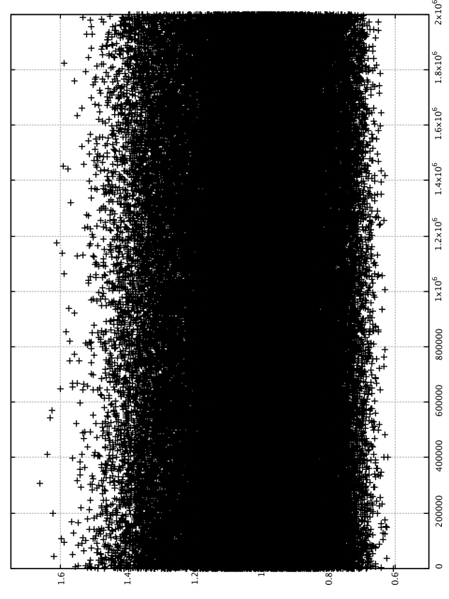
Figure 1. The values of $r(q)$, $q$ prime, $3\leq q\leq 2\cdot 10^{6}$, plotted using GNUPLOT, v.5.2, patchlevel 7. [max $=1.661436\dots$ attained at $q=305741$; min $=0.604599\dots$ attained at $q=3$; number of $r(q)>1$: $74795$ ($50.22$%); number of $r(q)<1$: $74137$; ($49.78$%) total number of data $=148932$].

We were able to compute the long double precision $r(q)$-values for every prime $3\leq q\leq 2\cdot 10^{6}$ and we provide here the scatter plot, see Figure 1, of such values. The minimal value is $r(3)=0.6045997880\dotsc$ and the maximal one is $r(305741)=1.661436\dotsc$ The data were obtained in about three days of computation time on the Dell OptiPlex machine mentioned before.

4.4. Computations for larger $q$.

If $bq+1$ is prime for many small $b,$ there is a good chance that $r(q)$ will be large. Promising, using this criterion, seemed $q=4178771$, $6766811$, $28227761$, $193894451$, $75743411$, $212634221$, $251160191$, $405386081$, $538906601$, $964477901$ and also $1139803271$, $1217434451$, $1806830951$, $2488788101$, $2830676081$, $2918643191.$ For these $q$ the $r(q)$’s were evaluated using the quadruple precision, see Table 3. We remark that the quadruple precision computation performances are affected by a lack of hardware support of the FLOAT128 type of the C programming language.

In Table 4 we evaluated some further cases with potential large $r(q)$ value: $q=4151292581$, $6406387241$, $7079770931$, $9854964401$ with the long double precision. These computations were performed on an Intel(R) Xeon(R) CPU E5-2650 v3 @ 2.30GHz, with 160 GB of RAM and running Ubuntu 16.04. The computation for $q=9109334831$ was performed on the CAPRI (“Calcolo ad Alte Prestazioni per la Ricerca e l’Innovazione”) infrastructure of the University of Padova.

The PARI/Gp scripts and the C programs used and the computational results obtained are available at the following web address: http://www.math.unipd.it/~languasc/rq-comput.html.

5. Further computation on the Euler-Kronecker constants

The Euler-Kronecker constant for the prime cyclotomic field $\mathbb{Q}(\zeta_{q})$ and for $\mathbb{Q}(\zeta_{q}+\zeta_{q}^{-1})$, the maximal real subfield of $\mathbb{Q}(\zeta_{q})$, see, e.g., [8], are defined as

$$\mathfrak{G}_{q}:=\gamma+\sum_{\chi\neq\chi_{0}}\frac{L^{\prime}(1,\chi)}{L(1,\chi)},\qquad\textrm{respectively}\qquad\mathfrak{G}_{q}^{+}:=\gamma+\sum_{\begin{subarray}{c}\chi\neq\chi_{0}\\ \chi\,\textrm{even}\end{subarray}}\frac{L^{\prime}(1,\chi)}{L(1,\chi)}.$$ (13)

Using formula (22) of [8] we have that

$$\mathfrak{G}_{q}-\mathfrak{G}_{q}^{+}=\sum_{\chi\,\textrm{odd}}\frac{L^{\prime}(1,\chi)}{L(1,\chi)}=\frac{q-1}{2}\Bigl{(}\gamma+\log(2\pi)\Bigr{)}+\sum_{\chi\,\textrm{odd}}\frac{1}{B_{1,\overline{\chi}}}\sum_{a=1}^{q-1}\overline{\chi}(a)\log\Bigl{(}\Gamma(\frac{a}{q})\Bigr{)},$$ (14)

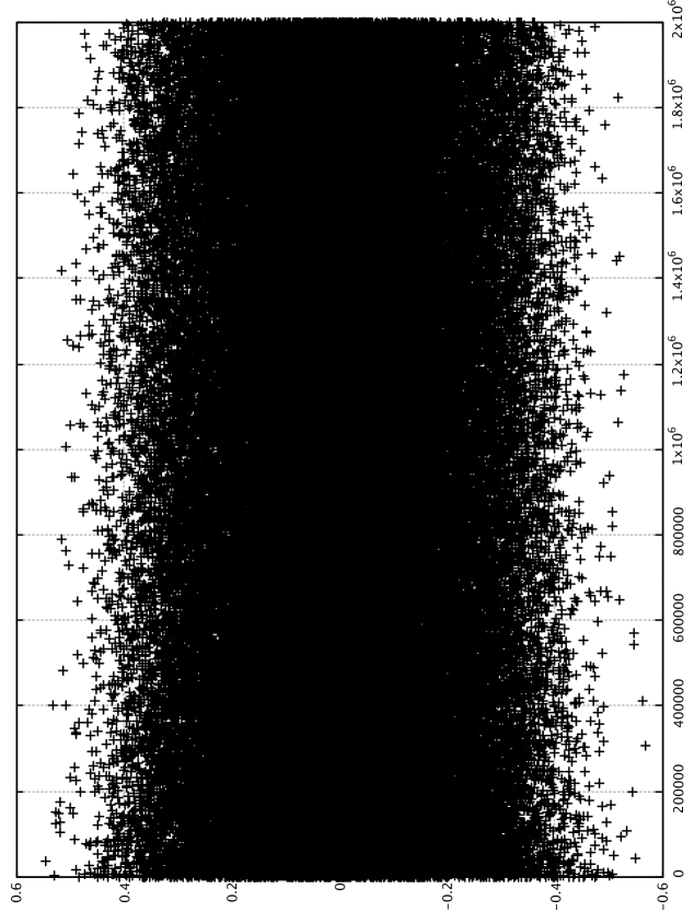
Figure 2. The values of $(\mathfrak{G}_{q}-\mathfrak{G}_{q}^{+})/\log q$, $q$ prime, $3\leq q\leq 2\cdot 10^{6}$, plotted using GNUPLOT, v.5.2, patchlevel 7. [ max $=0.546473\dots$ attained at $q=37189$; min $=-0.569200\dots$ attained at $q=305741$; number of positive data $=74190$ ($49.81$%); number of negative data $=74742$ ($50.19$%); total number of data $=148932$].

which can be easily implemented since the function $\log\Gamma$ is available in the C programming language. The scatter plot of Figure 2 represents the normalized values of $\mathfrak{G}_{q}-\mathfrak{G}_{q}^{+}$, $q$ prime, $3\leq q\leq 2\cdot 10^{6}$ and creating it took about three days on the Dell Optiplex machine mentioned before.

Since in (14) we can use a decimation in frequency strategy, we also remark that letting $f=\log\Gamma$ into (12) leads to simplify the form of $c_{k}=e(-k/(q-1))\bigl{(}\log\Gamma(a_{k}/q)-\log\Gamma(a_{k+m}/q)\bigr{)}$, where $m=(q-1)/2$ and $k=0,\dotsc,m-1$, in the following way. Recalling $\langle g\rangle=\mathbb{Z}^{*}_{q}$, $a_{k}\equiv g^{k}\bmod q$ and $g^{m}\equiv q-1\bmod{q}$, we can write that

$$\log\Bigl{(}\Gamma\bigl{(}\frac{a_{k+m}}{q}\bigr{)}\Bigr{)}=\log\Bigl{(}\Gamma\bigl{(}\frac{q-a_{k}}{q}\bigr{)}\Bigr{)}=\log\Bigl{(}\Gamma\bigl{(}1-\frac{a_{k}}{q}\bigr{)}\Bigr{)}$$

and hence, using the well-known reflection formula $\Gamma(x)\Gamma(1-x)=\pi/\sin(\pi x)$, we obtain

$$\log\Bigl{(}\Gamma\bigl{(}\frac{a_{k}}{q}\bigr{)}\Bigr{)}-\log\Bigl{(}\Gamma\bigl{(}1-\frac{a_{k}}{q}\bigr{)}\Bigr{)} =2\log\Bigl{(}\Gamma\bigl{(}\frac{a_{k}}{q}\bigr{)}\Bigr{)}+\log\Bigl{(}\sin\bigl{(}\frac{\pi a_{k}}{q}\bigr{)}\Bigr{)}-\log\pi,$$

for every $k=0,\dotsc,m-1$, $m=(q-1)/2$. Inserting the last relation in the definition of $c_{k}$ in (12) we obtain the actual sequence we used for performing the computation previously mentioned.

Acknowledgements. Part of the calculations described here were performed using the University of Padova Strategic Research Infrastructure Grant 2017: “CAPRI: Calcolo ad Alte Prestazioni per la Ricerca e l’Innovazione”. The first author, A. Languasco, thanks Luca Righi (University of Padova) for his help in using CAPRI. The second and fourth authors, P. Moree and A. Sedunova, thank the Max Planck Institute for Mathematics for providing excellent conditions while they were working on the project this paper is part of. The third author, S. Saad Eddin, is supported by the Austrian Science Fund (FWF): Project F5505-N26 and Project F5507-N26, which are part of the special Research Program “Quasi Monte Carlo Methods: Theory and Application”.

$q$	$r(q)$
$3$	$0.60459978807807261686469275254\dotsc$
$5$	$0.78956835208714868950675927999\dotsc$
$7$	$0.95667518575084187547950733813\dotsc$
$11$	$1.10916191287000575896982175317\dotsc$
$13$	$1.07714905620985756748597815892\dotsc$
$17$	$0.85539034568765268115905873936\dotsc$
$19$	$0.70704004900384729070674621978\dotsc$
$23$	$1.27303069939685502234405162961\dotsc$
$29$	$1.19507225854723141702138692301\dotsc$
$31$	$0.88988962107854407891985181571\dotsc$
$37$	$0.89617354245182624263930105684\dotsc$
$41$	$1.01095149281551337376703651618\dotsc$
$43$	$1.00032807083987921579084335194\dotsc$
$47$	$0.99510419475843763320461794597\dotsc$
$53$	$1.00231549556080469808835403497\dotsc$
$59$	$1.03111995957758588341749868917\dotsc$
$61$	$0.91541689757636152038607840584\dotsc$
$67$	$1.03230196304201968151553976333\dotsc$
$71$	$0.94652474710362368092900546271\dotsc$
$73$	$1.28217793230760538382246761185\dotsc$
$79$	$0.84579459612002975504552940763\dotsc$
$83$	$1.22326926548441461619507621390\dotsc$
$89$	$1.28632147461922346234453694590\dotsc$
$97$	$0.90467614287023765066781857933\dotsc$
$101$	$1.11049958753586448051923888082\dotsc$
$103$	$1.05565198833718743186163713482\dotsc$
$107$	$0.99260767792672501309519612375\dotsc$
$109$	$0.91554283885230186850667500246\dotsc$
$113$	$1.16185573635061808057761114590\dotsc$
$127$	$1.06269835499717635407980190888\dotsc$
$131$	$1.27897699389762867270592988247\dotsc$
$137$	$1.00188853650420792851571142833\dotsc$
$139$	$0.87166115187392327886708542130\dotsc$
$149$	$1.04886527642691194564791006449\dotsc$
$151$	$1.09613526050530812035603232922\dotsc$
$157$	$0.74304505329108896600523002862\dotsc$
$163$	$0.95167392369442992883081838307\dotsc$
$167$	$0.85404891714098835186838607451\dotsc$
$173$	$1.25750311100604863256476652232\dotsc$
$179$	$1.31898955218699008540672120548\dotsc$
$181$	$1.01646725307901783240856438797\dotsc$
$191$	$1.29850955347246763676155271715\dotsc$
$193$	$1.17384956614280523683625176108\dotsc$
$197$	$0.87142685805870225854275086741\dotsc$
$199$	$0.79775765981803261703336410970\dotsc$
$211$	$0.70965810384577007739153826881\dotsc$
$223$	$0.90016736774009107389420074861\dotsc$
$227$	$0.76298839763137122603762871170\dotsc$
$229$	$0.72414574142010494620086404196\dotsc$
$233$	$1.43102216731058063469583770264\dotsc$
$239$	$1.18520259221018381028526578871\dotsc$
$241$	$1.11908192699651325481120769078\dotsc$
$251$	$1.18041694425392859170387583509\dotsc$
$257$	$0.90559625735496576640913464538\dotsc$
$263$	$0.93717078166852960654064932319\dotsc$
$269$	$1.01052429941342866041104883014\dotsc$

$q$	$r(q)$
$271$	$0.84120880901441103034587178906\dotsc$
$277$	$1.22287167700803659996325347046\dotsc$
$281$	$1.09072312671446411507457756821\dotsc$
$283$	$0.98730045924989351176735192970\dotsc$
$293$	$1.28843023595237283191056798455\dotsc$
$307$	$0.91358725220199482220514916899\dotsc$
$311$	$1.14589374542647302213444142687\dotsc$
$313$	$0.93893317675819166180673984422\dotsc$
$317$	$0.80671823188984812849457198577\dotsc$
$331$	$0.81356274956051845902331649336\dotsc$
$337$	$0.86111511521922591268832255791\dotsc$
$347$	$1.08517941758105267446483313058\dotsc$
$349$	$0.98395731344877010445591239132\dotsc$
$353$	$0.88603505661744604503087815775\dotsc$
$359$	$1.16002644446708254566916432735\dotsc$
$367$	$0.90864101877936912063265319825\dotsc$
$373$	$1.07507614420133257646267035535\dotsc$
$379$	$0.72144618647138444694426995688\dotsc$
$383$	$0.83243809267428713960470760380\dotsc$
$389$	$0.84997782896854503971627563496\dotsc$
$397$	$0.99757781120158579094253246616\dotsc$
$401$	$1.13998328316447070631384278931\dotsc$
$409$	$1.19919809743909540748744244798\dotsc$
$419$	$1.18974458882376935926766971002\dotsc$
$421$	$0.86457966530711741177342869535\dotsc$
$431$	$1.13754261103593462461717085623\dotsc$
$433$	$1.07176135182041771385450595205\dotsc$
$439$	$0.68484134061729762055005895626\dotsc$
$443$	$1.41089988430397986980906568345\dotsc$
$449$	$0.90539643658614424895891547460\dotsc$
$457$	$0.83734634190585621778636791343\dotsc$
$461$	$1.03119557377397403645284724907\dotsc$
$463$	$0.96134625111959841778686635231\dotsc$
$467$	$0.89740454859192836870657083737\dotsc$
$479$	$1.10506715780642069705910978939\dotsc$
$487$	$1.13041022782656063139453697156\dotsc$
$491$	$1.27221465691304968352754354985\dotsc$
$499$	$0.82979024959465063669881382680\dotsc$
$503$	$1.09956174719578329093362210466\dotsc$
$509$	$1.39692082719612661320417410651\dotsc$
$521$	$0.74488579181918272860910159248\dotsc$
$523$	$0.99514847873992894203802693220\dotsc$
$541$	$0.94472655782952981521345779529\dotsc$
$547$	$0.73868505476195458996166613201\dotsc$
$557$	$1.01800618130970440243478675140\dotsc$
$563$	$0.92322125091337523644162001846\dotsc$
$569$	$0.86644384514357385272705168284\dotsc$
$571$	$0.99662480636851972762309151349\dotsc$
$577$	$0.91370293804018510239277389204\dotsc$
$587$	$0.81252459850672121660374173954\dotsc$
$593$	$1.07734617489664930780759188442\dotsc$
$599$	$0.96408773834723069779571268471\dotsc$
$601$	$0.92827339751824097250854300550\dotsc$
$607$	$0.83637312705251443247667799101\dotsc$
$613$	$0.87703659303472148910355020294\dotsc$
$617$	$0.84246084541946716141445378848\dotsc$

$q$	$r(q)$
$619$	$0.80463918636548231818097049238\dotsc$
$631$	$1.13964698072442766479584447731\dotsc$
$641$	$1.34299156432328475445263673245\dotsc$
$643$	$1.01836205611360685304417553494\dotsc$
$647$	$0.90233667317118875595490772209\dotsc$
$653$	$1.27087727805772466468796098338\dotsc$
$659$	$1.39106317898226550143998268526\dotsc$
$661$	$0.83544430975232146569368385972\dotsc$
$673$	$1.03660206982398637181187353211\dotsc$
$677$	$0.92424013312497364401792044662\dotsc$
$683$	$1.13528281402409476998254691134\dotsc$
$691$	$0.76921427957454050696406411036\dotsc$
$701$	$0.92089882867969861041626254382\dotsc$
$709$	$1.05648934917801861606174800341\dotsc$
$719$	$1.20306325855333927681117243729\dotsc$
$727$	$0.99856921422780328631340639607\dotsc$
$733$	$0.98014910177261986736078022621\dotsc$
$739$	$1.10263546824053086630671245464\dotsc$
$743$	$1.03495494096205775904091176831\dotsc$
$751$	$1.01856200583585073878095848975\dotsc$
$757$	$0.96706876118708598545541455447\dotsc$
$761$	$1.46958285813141552491322656984\dotsc$
$769$	$0.89892230367392111314972716474\dotsc$
$773$	$1.06810947197031447130333305035\dotsc$
$787$	$0.97178232843986336686451556474\dotsc$
$797$	$1.03075130387360942943641986527\dotsc$
$809$	$1.31970441406018712251949567645\dotsc$
$811$	$0.80283817264815420707856818905\dotsc$
$821$	$1.06528437036549643319352814656\dotsc$
$823$	$0.96769318476182048656465705918\dotsc$
$827$	$0.86555993675758442057691969953\dotsc$
$829$	$0.82250033541615549748400919644\dotsc$
$839$	$0.91871090540765761610044317666\dotsc$
$853$	$1.08223582880253347548004283614\dotsc$
$857$	$1.05075311490694694576396382027\dotsc$
$859$	$0.88080094180568178476397675721\dotsc$
$863$	$1.05694231206444764180240401289\dotsc$
$877$	$0.72289398522705741218284637854\dotsc$
$881$	$1.09738994199075350184435336371\dotsc$
$883$	$1.13318227639393214982039012685\dotsc$
$887$	$0.96917974196790823108417719936\dotsc$
$907$	$0.90262558866311480478051623607\dotsc$
$911$	$1.07798557536304873099351043701\dotsc$
$919$	$1.04003346554199950901317303457\dotsc$
$929$	$1.04414904452989167744813201725\dotsc$
$937$	$0.90017934857750019784132262523\dotsc$
$941$	$1.09400867179752235523397214847\dotsc$
$947$	$1.22587448270510743026091490433\dotsc$
$953$	$1.16083173031283885682226845601\dotsc$
$967$	$0.72860004404668861481436825047\dotsc$
$971$	$1.07939115916440046258710381604\dotsc$
$977$	$0.83890885880371282354125472475\dotsc$
$983$	$0.78867677202973854047246566763\dotsc$
$991$	$0.90943936153505129760069639750\dotsc$
$997$	$0.85575754491350654466545217865\dotsc$

Table 1. Values of $r(q)$ for every odd prime up to $1000$ with a precision of $30$ digits; computed with PARI/Gp, v. 2.11.2, with a trivial way of executing the sum over $a$. Total computation time: 8s., 947ms. using the first $\chi$-Bernoulli number. [s=seconds; msec=milliseconds]

$q$	$r(q)$	time $\psi$-version	time Bernoulli-version	time direct version
$1451$	$1.489316072\dotsc$	292ms.	299ms.	2s. 083ms.
$2741$	$1.498121015\dotsc$	1s. 019ms.	1s. 061ms.	5s. 231ms.
$3331$	$0.642429297\dotsc$	1s. 496ms.	1s. 566ms.	7s. 236ms.
$4349$	$1.518570512\dotsc$	2s. 536ms.	2s. 657ms.	10s. 572ms.
$4391$	$1.507776410\dotsc$	2s. 586ms.	2s. 710ms.	11s. 276ms.
$5231$	$1.556562248\dotsc$	3s. 361ms.	3s. 385ms.	14s. 730ms.
$6101$	$1.511405291\dotsc$	4s. 964ms.	5s. 086ms.	17s. 490ms.
$6379$	$0.673523026\dotsc$	5s. 436ms.	5s. 699ms.	19s. 859ms.
$7219$	$0.658084090\dotsc$	6s. 978ms.	7s. 293ms.	23s. 966ms.
$8209$	$0.672045039\dotsc$	8s. 950ms.	9s. 416ms.	27s. 322ms.
$9049$	$0.667614244\dotsc$	10s. 870ms.	11s. 461ms.	32s. 610ms.
$9689$	$1.524371504\dotsc$	12s. 487ms.	13s. 113ms.	36s. 855ms.

Table 2. A few other values of $r(q)$ with a precision of $10$ digits; computed with PARI/Gp, v. 2.11.2, with a trivial way of executing the sum over $a$. [s=seconds; msec=milliseconds]

$q$	$r(q)$	total time	total time
		(long double)	(quadruple)
$4178771$	$1.611588128\dotsc$	2s. 471ms.	42s. 007ms.
$6766811$	$1.709379041\dotsc$	4s. 200ms.	1m. 01s. 314ms.
$28227761$	$1.528720351\dotsc$	16s. 267ms.	4m. 30s. 804ms.
$75743411$	$1.645759517\dotsc$	1m. 05s. 078ms.	19m. 04s. 250ms.
$193894451$	$1.548501406\dotsc$	2m. 18s. 739ms.	38m. 27s. 838ms.
$212634221$	$1.652149469\dotsc$	2m. 44s. 018ms.	48m. 24s. 277ms.
$251160191$	$1.611898472\dotsc$	3m. 02s. 783ms.	54m. 20s. 875ms.
$405386081$	$1.545118923\dotsc$	4m. 31s. 634ms.	58m. 49s. 163ms.
$538906601$	$1.693680145\dotsc$	6m. 44s. 584ms.	114m. 59s. 330ms.
$964477901$	$1.612596619\dotsc$	12m. 21s. 793ms.	217m. 40s. 768ms.
$1139803271$	$1.398836497\dotsc$	21m. 56s. 349ms.	298m. 29s. 058ms.
$1217434451$	$1.707310115\dotsc$	15m. 00s. 374ms.	277m. 58s. 390ms.
$1806830951$	$1.621464926\dotsc$	23m. 00s. 240ms.	417m. 46s. 183ms.
$2488788101$	$1.662760638\dotsc$	29m. 54s. 639ms.	512m. 29s. 915ms.
$2830676081$	$1.616923086\dotsc$	32m. 46s. 208ms.	552m. 42s. 941ms.
$2918643191$	$1.693092857\dotsc$	38m. 40s. 423ms.	697m. 10s. 305ms.

Table 3. Few other values of $r(q)$; computed using the first $\chi$-Bernoulli number with PARI/Gp, v. 2.11.2. and fftw, v. 3.3.8., with long double and quadruple precisions. The sum over $a$ was performed using the FFT algorithm on the Xeon machine mentioned before. [m=minutes; s=seconds; msec=milliseconds, n.a.=not available]

$q$	$r(q)$	total time (long double)
$4151292581$	$1.669735\dotsc$	63m. 00s.
$6406387241$	$1.625741\dotsc$	75m. 38s.
$7079770931$	$1.688607\dotsc$	187m. 20s.
$9109334831$	$1.657855\dotsc$	120m. 28s.
$9854964401$	$1.688033\dotsc$	177m. 14s.

Table 4. Few other values of $r(q)$; computed using the first $\chi$-Bernoulli number with PARI/Gp, v. 2.11.2. and fftw, v. 3.3.8., with long double precision. The sum over $a$ was performed using the FFT algorithm on the Xeon machine mentioned before with the only exception of $q=9109334831$ for which we used the CAPRI infrastructure of the University of Padova. [m=minutes; s=seconds]

1223

References

- [1] H. Cohen, Number Theory. Volume II: Analytic and Modern Tools, Graduate Texts in Mathematics, vol. 240, Springer, 2007.
- [2] K. Ford, F. Luca, P. Moree, Values of the Euler -function not divisible by a given odd prime, and the distribution of Euler-Kronecker constants for cyclotomic fields, Math. Comp. 83 (2014), 1447–1476.
- [3] M. Frigo, S. G. Johnson, The Design and Implementation of FFTW3, Proceedings of the IEEE 93 (2), 216–231 (2005). The C library is available at http://www.fftw.org.
- [4] G. Fung, A. Granville, H. C. Williams, Computation of the first factor of the class number of cyclotomic fields, J. Number Theory 42 (1992), 297–312.
- [5] Gnu Scientific Library, version 2.5, 2018. Available from http://www.gnu.org/software/gsl/.
- [6] H. Hasse, Über die Klassenzahl abelscher Zahlkörper, Akademie-Verlag, Berlin, 1952, reprinted with an introduction by J. Martinet, Springer-Verlag, 1985.
- [7] E. E. Kummer, Memoire sur la théorie des nombres complexes composes de racines de l’unité et des nombres entiers, J. Math. Pures Appl. (1851), 377–498, reprinted in his Collected papers, Vol. I, Springer-Verlag, 1975, pp. 363–484.
- [8] A. Languasco, A note on the computation of the Euler-Kronecker constants for prime cyclotomic fields, Arxiv, 2019, http://arxiv.org/abs/1903.05487.
- [9] P. Moree, Irregular Behaviour of Class Numbers and Euler-Kronecker Constants of Cyclotomic Fields: The Log Log Log Devil at Play, Irregularities in the Distribution of Prime Numbers. From the Era of Helmut Maier’s Matrix Method and Beyond (J. Pintz and M.Th. Rassias, eds.), Springer, 2018, pp. 143–163.
- [10] The PARI Group, PARI/GP version 2.11.2, Bordeaux, 2019. Available from http://pari.math.u-bordeaux.fr/.
- [11] C. M. Rader, Discrete Fourier transforms when the number of data samples is prime, Proc. IEEE 56 (1968), 1107–1108.
- [12] M. A. Shokrollahi, Relative class number of imaginary abelian fields of prime conductor below , Math. Comp. 68 (1999), 1717–1728.