A Gray Level Indicator-Based Regularized Telegraph Diffusion Equation Applied to Image Despeckling

Abstract

In this work, a gray level indicator based non-linear telegraph diffusion model is presented for multiplicative noise removal problem. Most of the researchers focus only on diffusion equation-based model for multiplicative noise removal problem. The suggested model uses the benefit of the combined effect of diffusion equation as well as the wave equation. Wave nature of the model preserves the high oscillatory and texture pattern in an image. In this model, the diffusion coefficient depends not only on the image gradient but also on the gray level of the image, which controls the diffusion process better than only gradient-based diffusion models. Moreover, we prove the well-posedness of the present model using Schauder fixed point theorem. Furthermore, we show the superiority of the proposed model over a recently developed method on a set of gray level test images which are corrupted by speckle noise.

Keywords Speckle noise  $\cdot$ Despeckling  $\cdot$ Telegraph diffusion equation  $\cdot$ Gray level indicator  $\cdot$ Weak solution  $\cdot$ Schauder fixed point theorem.

1 Introduction

In the real scenario, images are often corrupted by different types of noises, e.g., additive, multiplicative, or mixed nature. Hence the noise removal process is a very initial stage for high-level image analysis. In this work, we focus our interest only on multiplicative speckle noise removal process. Purity of the edge/texture information in the synthetic aperture radar(SAR) images, ultrasound images, and laser images are usually diminished by speckle noise [10, 37, 41]. Due to the contamination by speckle noise, it is challenging to distinguish the hidden details in the images. Therefore the development of an advance speckle noise removal algorithm is always an essential aspect for the image processing society. A Mathematical representation is still required to develop an efficient noise removal algorithm so that we can express each pixel of an image as a function of the speckle noise. The popularly used model for the noise image can be express as a product of the original signal and the speckle noise [17]

$$J=I\eta,$$

where $J$ indicates the noisy image, $I$ is the noise-free image, and $\eta$ signifies the speckle-noise process.

In general, the probability density function of the multiplicative speckle noise process $\eta$ follows the Gamma Law as,

$$g(\eta)=\begin{cases}\frac{L^{L}}{\Gamma\left(L\right)}\eta^{L-1}\text{exp}\left(-L\eta\right),\hskip 14.22636pt\text{for}\hskip 2.84544pt\eta>0,\\ \hskip 42.67912pt0,\hskip 54.06006pt\text{for}\hskip 2.84544pt\eta=0,\end{cases}$$

where $L\in{\rm I\!N}$ signifies the number of looks which correspond to the noise level in the corrupted images [7, 22, 35] and $\Gamma\left(\cdot\right)$ denotes the Gamma function.

A large number of study reports the fundamentals and the statistical attributes of the speckle noise [1, 7, 19, 32, 33, 41]. Futuristic despeckling approaches include Bayesian methods in spatial domain [19, 32, 33], Bayesian methods in transformed domain [4, 21, 39], order-statistics and morphological filters [6, 5, 14, 41], simulated annealing despeckling [50], nonlocal filtering [9, 13, 15, 48], wavelet-based approaches [1, 46], nonlinear diffusion in Laplacian pyramid domain [53], anisotropic diffusion based methods [25, 27, 29, 44, 52, 55, 56], and variational methods [8, 16, 23, 28, 30, 31, 36, 43, 45].

From the initiation of PM model [40], the partial differential equations(PDEs) are extensively used to develop noise removal algorithms, among different types of PDE based models, the total variational (TV) based algorithms are achieved remarkable results. First variational based strategy to deal with multiplicative noise is proposed by Rudin et al. [43], with the principles,

$$\int_{\Omega}\frac{J}{I}dx=1,\quad{\rm and}\quad\int_{\Omega}{\left(\frac{J}{I}-1\right)}^{2}dx=\sigma^{2}\,,$$

where $\sigma^{2}$ represents the variance of the noise $\eta$. Due to the non-convexity of their proposed energy function, the model may not give a globally unique solution. To succeed over this shortcoming, several authors suggested various convex functional with different data fidelity terms [8, 23, 31, 36]. Recently, Dong et al. [16] suggest a convex total variation model for multiplicative speckle-noise reduction with the following form:

$$I=\min_{I\in\text{BV}\left(\Omega\right)}\left\{\int_{\Omega}\alpha(x)|\nabla I|dx+\lambda\int_{\Omega}\left(I+J\log\frac{1}{I}\right)dx\right\}.$$

They choose the gray level indicator function $\alpha$, as

$$\left(1-\frac{1}{1+k|G_{\xi}\ast J|^{2}}\right)\frac{1+kM^{2}}{kM^{2}},\,\,\,\,\text{or}\,\,\,\,\,\dfrac{G_{\xi}\ast J}{M},$$

with $M=\underset{x\in\Omega}{\text{sup}}(G_{\xi}\ast J)(x)$, where $\xi>0$, $k>0$, “$\ast$" is the convolution operator, $G_{\xi}$ is the two dimensional Gaussian kernel and $\lambda$ is a given parameter, see [16]. Later, based on a gray level indicator function, Zhou et al. proposed a diffusion model (DDD model)[55] for multiplicative noise removal problem. Their model takes the form:

$$I_{t}=\text{div}(g(I,|\nabla I|)\nabla I),\hskip 8.5359pt\text{in}\hskip 5.69046pt\Omega_{T}:=\Omega\times(0,T),$$

$$\partial_{n}I=0,\hskip 73.97733pt\text{in}\hskip 5.69046pt\partial\Omega_{T}:=\partial\Omega\times(0,T),$$

$$I(x,0)=I_{0}(x),\hskip 42.67912pt\text{in}\hskip 5.69046pt\Omega,$$

where $\Omega$ is the domain of original image $I$ and the observed noise image $I_{0}$, div and $\nabla$ represents the divergence and gradient operator respectively. They choose the diffusion coefficient as

$$g\left(I,|\nabla I|\right)=\dfrac{2|I|^{\nu}}{M^{\nu}+|I|^{\nu}}\cdot\dfrac{1}{\left(1+|\nabla I|^{2}\right)^{(1-\beta)/2}},$$

where $\nu>0,$ $0<\beta<1,$ and $M=\underset{x\in\Omega}{\text{sup}}I$. In this case, the gray level indicator and edge detector function are $a(I):=\dfrac{2|I|^{\nu}}{M^{\nu}+|I|^{\nu}}$ and $b(I):=\dfrac{1}{\left(1+|\nabla I|^{2}\right)^{(1-\beta)/2}}$ respectively. However because of the degeneracy of the edge detector function, i.e., $b(|\nabla I|)\rightarrow 0$ as $|\nabla I|\rightarrow\infty$, it is challenging to establish the well-posedness of their model. Recently Shan et al. [44] proposed a regularized version of the above-discussed model [55]. In [44], the model takes of the form

$$I_{t}=\text{div}(g(I_{\xi},|\nabla I_{\xi}|)\nabla I),\hskip 5.69046pt\text{in}\hskip 5.69046pt\Omega_{T},$$

$$\partial_{n}I=0,\hskip 73.97733pt\text{in}\hskip 5.69046pt\partial\Omega_{T},$$

$$I(x,0)=I_{0}(x),\hskip 42.67912pt\text{in}\hskip 5.69046pt\Omega\,.$$

They choose the diffusion coefficient as

$$g\left(I,|\nabla I|\right)=\left(\dfrac{I_{\xi}}{M_{\xi}^{I}}\right)^{\nu}\cdot\dfrac{1}{1+|\nabla I_{\xi}|^{\beta}},$$

where $I_{\xi}=G_{\xi}\ast I$, $M_{\xi}^{I}=\underset{x\in\Omega}{\text{max}}|I_{\xi}(x,t)|$, $I_{0}$ is the initial image, and $\nu,\beta$ and $\xi$ are positive constants. Due to the introduction of the Gaussian kernel in the diffusion coefficient, which avoids the degeneracy in the model, the authors able to study the wellposedness of the underlying problem.

To the best of our knowledge, most of the researcher concentrated their interest only on parabolic PDE based models, which are developed either from the variational bases approach or diffusion based approach, for the speckle-noise removal process. The hyperbolic PDEs could upgrade the quality of the detected edges and improve the image better than parabolic PDEs [2]. In the existing literature, the first hyperbolic model for image denoising is telegraph-diffusion model [42], where the image was viewed as an elastic sheet placed in a damping environment, which interpolates between the diffusion equation and the wave equation. The telegraph-diffusion model takes the form,

$$I_{tt}+\gamma I_{t}=\text{div}(g(|\nabla I|)\nabla I),\hskip 17.07182pt\text{in}\hskip 5.69046pt\Omega_{T},$$

$$\partial_{n}I=0,\hskip 99.58464pt\text{in}\hskip 5.69046pt\partial\Omega_{T},$$

$$I(x,0)=I_{0}(x),\hskip 5.69046ptI_{t}(x,0)=0,\hskip 8.5359pt\text{in}\hskip 5.69046pt\Omega,$$

where $g(|\nabla I|)=1/(1+({|\nabla I|^{2}}/{k^{2}}))$ is an edge-controlled diffusion function which preserves the important features and smoothen the unwanted signals, and $\gamma$ is the damping parameter. It is quite interesting to note that for a very higher value of $g$ and $\gamma$, this telegraph-diffusion equation (TDE model) converges to the original PM model [40] in a long time scenario. Although the TDE model performs better, it is challenging to confirm the well-posedness of their model. To overcome the ill-posedness issue in the TDE model [42], Cao et al. suggest a regularized TDE model [11]. They replace the gradient $|\nabla I|$ by $|\nabla G_{\xi}\ast I|$ in the edge-controlled function $g$ in the TDE model [42] and establish the well-posedness of their proposed model. Even though the TDE model can effectively preserve the sharp edges but failed to produce satisfactory smoothing in the presence of a large level of noise. To overcome this issue, several non-linear telegraph diffusion-based method have been proposed [11, 24, 47, 51, 54]. However, in spite of their impressive applications in the additive noise removal process, hyperbolic PDE based approaches have not successfully used for speckle noise removal process.

Recently Sudeb et al. suggest a fuzzy edge detector based telegraph total variation model [38] for the speckle noise removal problem. To the best of our knowledge, this is the first hyperbolic PDE based model in the existing literature applied to speckle noise removal process. The model [38] takes the form,

$$I_{tt}+\gamma I_{t}=\text{div}\left(\theta(I)\frac{\nabla I}{|\nabla I|}\right)-\lambda\left(1-\frac{I_{0}}{I}\right),\hskip 17.07182pt\text{in}\hskip 5.69046pt\Omega_{T},$$

$$\partial_{n}I=0,\hskip 173.56198pt\text{in}\hskip 5.69046pt\partial\Omega_{T},$$

$$I(x,0)=I_{0}(x),\hskip 2.84544ptI_{t}(x,0)=0,\hskip 85.35826pt\text{in}\hskip 5.69046pt\Omega,$$

where $\theta$ is the fuzzy edge detector function [12], $\gamma$ is a positive parameter and $\lambda$ is the weight parameter.

Further continuing to demonstrate the importance of hyperbolic PDE based model for image despeckling, the present work suggests a gray level indicator based telegraph diffusion model for multiplicative speckle noise removal. In this model, we choose a different diffusivity function from our previous model [38]. Also, instead of total variation framework [38], we designed the present model in an anisotropic diffusion-based fashion as discussed in [55]. Furthermore, we study the well-posedness of the suggested model in an appropriate function space. We opt an explicit numerical method to solve the present model. Our numerical implementation allows computing despeckled results on some standard test images. Quality of the despeckled images using the suggested model compare with the recently developed model [44]. We compare the quantitative and qualitative results at different noise levels. The experiment results confirm that the proposed model performs better as compared to the model considered for the comparison.

The rest of the paper is organized as follows. Section 2 describes the proposed telegraph diffusion method for image despeckling. In section 3, we study the wellposedness of weak solution of the proposed model. Section 4 describes the numerical discretization of the present model. The simulated despeckling results obtained by the proposed approach are compared with other discussed diffusion methods in Section 5. We conclude the paper in Section 6 with a scope on future work.

2 Telegraph Diffusion Model for Speckle Noise Removal

Inspired by the ideas of [38] and [55] initially we developed the model

$$I_{tt}+\gamma I_{t}-\text{div}\left(g\left(I,|\nabla I|\right)\nabla I\right)=-\lambda h(I_{0},I)\,,\hskip 5.69046pt\text{in}\,\,\,\Omega_{T}\,,$$ (2.1)

$$\partial_{n}I=0\,,\hskip 162.18062pt\text{on}\,\,\,\partial\Omega_{T}\,,$$ (2.2)

$$I(x,0)=I_{0}(x)\,,\hskip 5.69046ptI_{t}(x,0)=0\,,\hskip 71.13188pt\text{in}\,\,\,\Omega\,.$$ (2.3)

The function $g$ is defined as

$$g\left(I,|\nabla I|\right)=\dfrac{2|I|^{\nu}}{\big{(}M^{I}\big{)}^{\nu}+|I|^{\nu}}.\dfrac{1}{1+\left(\frac{|\nabla I|}{K}\right)^{2}},$$ (2.4)

where, $\nu\geq 1,$ $\gamma,K>0$ are constants, $M^{I}=\underset{x\in\Omega}{\text{max}}|I(x,t)|$, and $h(I_{0},I)$ is the source term which comes due to the fidelity control term in the energy functional as discussed in [38]. Although the presence of fidelity term in the equation keeps the restored image close to the original image, the noise may not be removed sufficiently. Therefore we would like to choose $h(I_{0},I)=0.$ Also, because of the degeneracy in the diffusion coefficient 2.4, the suggested model (2.1)-(2.3) may not be a well-posed problem[44]. To overcome these issues, we invoke the ideas of [11] and [44], and finally designe the following model in the anisotropic diffusion-based framework:

$$I_{tt}+\gamma I_{t}-\text{div}\left(g\left(I_{\xi},|\nabla I_{\xi}|\right)\nabla I\right)=0\,,\hskip 31.2982pt\text{in}\,\,\,\Omega_{T}\,,$$ (2.5)

$$\partial_{n}I=0\,,\hskip 153.6447pt\text{on}\,\,\,\partial\Omega_{T}\,,$$ (2.6)

$$I(x,0)=I_{0}(x)\,,\hskip 5.69046ptI_{t}(x,0)=0\,,\hskip 62.59596pt\text{in}\,\,\,\Omega\,,$$ (2.7)

where the diffusion function $g$ as given by

$$g\left(I_{\xi},|\nabla I_{\xi}|\right)=\dfrac{2|I_{\xi}|^{\nu}}{\big{(}M^{I}_{\xi}\big{)}^{\nu}+|I_{\xi}|^{\nu}}\cdot\dfrac{1}{1+\left(\frac{|\nabla I_{\xi}|}{K}\right)^{2}}\,.$$

In the above, $I_{\xi}=G_{\xi}\ast I$, $M^{I}_{\xi}=\underset{x\in\Omega}{\text{max}}|I_{\xi}(x,t)|.$ Moreover the gray level indicator function

$$b(I)=\dfrac{2|I_{\xi}|^{\nu}}{\big{(}M^{I}_{\xi}\big{)}^{\nu}+|I_{\xi}|^{\nu}}$$

can be transformed into $b(s)=\dfrac{2s^{\nu}}{1+s^{\nu}}$, where $s=\dfrac{|I_{\xi}|}{M_{\xi}^{I}}\in[0,1].$

The use of Gaussian convolution in the proposed model has a lot of advantages, not only the robustness in denoising viewpoint but also the well-posedness in the theoretical perspective. There are two key advantages of this proposed approach:

• it provides the sharp and true edges during noise removal process than other non-telegraph based algorithms as the model (2.5)-(2.7) consists of telegraph diffusion model [42]

• it controls the diffusion process very well along with the gradient based edge detector coefficient specially for the speckle noise removal process [16] as the gray level indicator function in the proposed model is incorporated into the telegraph diffusion framework.

3 Wellposedness of weak solution

In this section, we prove the existence and uniqueness of weak solution of the proposed model (2.5)-(2.7). Since the problem (2.5)-(2.7) is nonlinear, we first consider the linearized problem, and then use Schauder’s fixed-point theorem [18] to show the existence of a weak solution. Without loss of generality, we assume $\gamma=1$ in (2.5).

3.1 Technical framework $\&$ statement of the main result

Throughout this section, $C$ denotes a generic positive constant. For $1\leq p\leq\infty$, we denote by $(L^{p},\|\cdot\|_{L^{p}})$ the standard spaces of $p$-th order integrable functions on $\Omega$. For $r\in\mathbb{N}$, we write $(H^{r},\|\cdot\|_{H^{r}})$ for usual Sobolev spaces on $\Omega$, and $(H^{1})^{\prime}$ for the dual space of $H^{1}$. We introduce the solution space $W(0,T)$ for the problem (2.5)-(2.7), where

$$W(0,T) =\Big{\{}w\in L^{\infty}(0,T;H^{1})\,,w_{t}\in L^{\infty}(0,T;L^{2});\,w_{tt}\in L^{2}(0,T;(H^{1})^{\prime})\Big{\}}\,.$$

Note that the space $W(0,T)$ is a Hilbert space for the graph norm, see [34].

Definition 3.1 (Weak solution)

A function $I$ is called a weak solution of (2.5)-(2.7) if

• $I\in W(0,T)$ and (2.7) holds.

• For all $\phi\in H^{1}$ and a.e $t\in(0,T)$, there hold

  $$\left\langle I_{tt},\phi\right\rangle+{\displaystyle\int_{\Omega}}\Big{(}I_{t}\phi+g\left(I_{\xi},|\nabla I_{\xi}|\right)\nabla I\cdot\nabla\phi\Big{)}\,dx=0.$$

As we mentioned, our aim is to establish wellposedness of weak solutions of the underlying problem (2.5)-(2.7), and we will do so under the following assumption:

1. The initial data $I_{0}$ is an $H^{2}$-valued function such that

   $$0<\alpha:=\inf_{x\in\Omega}I_{0}(x)\,.$$

Theorem 3.1

Let the assumption A.1 be true. Then the problem (2.5)-(2.7) admits a unique weak solution in the sense of Definition 3.1.

3.2 Linearized problem $\&$ existence of weak solution:

For any positive constant $M_{1}>0$, define

$$W_{M_{1}}=\big{\{} \bar{I}\in W(0,T):~{}\|\bar{I}\|_{L^{\infty}(0,T;H^{1})}+\|\bar{I}_{t}\|_{L^{\infty}(0,T;L^{2})}\leq M_{1}\|I_{0}\|_{H^{1}},\,$$

$$\hskip 14.22636pt0<\alpha\leq\bar{I}(x,t)~{}~{}{\rm for~{}a.e.}~{}~{}(x,t)\in\Omega_{T}\,\big{\}}.$$

For any $\bar{I}\in W_{M_{1}}$, consider the linearized problem:

$$I_{tt}+I_{t}-{\rm div}\big{(}\bar{g}(x,t)\nabla I\big{)}=0\hskip 28.45274pt{\rm in}~{}~{}~{}\Omega_{T}\,,$$ (3.1)

with the initial condition (2.7), where the function $\bar{g}$ is given by

$$\bar{g}(x,t)\equiv g_{\bar{I}}(x,t):=\frac{|\bar{I}_{\xi}|^{\nu}}{\big{(}M_{\xi}^{\bar{I}}\big{)}^{\nu}+|\bar{I}_{\xi}|^{\nu}}\cdot\dfrac{1}{1+\left(\frac{|\nabla\bar{I}_{\xi}|}{K}\right)^{2}}\,.$$

Claim 3.1

There exist positive constants $\kappa,C>0$, depending only on $G_{\xi},I_{0},M_{1},K,\alpha$ and $\nu$, such that

$${\rm i)}~{}0<\kappa\leq\bar{g}\leq 1\,,$$ (3.2)

$${\rm ii)}~{}|\bar{g}_{t}|\leq C\,.$$

Proof: Proof of ${\rm i)}$: Since $\bar{I}\in W_{M_{1}}$, by convolution property, we have

$$\alpha\|G_{\xi}\|_{L^{1}}\leq|G_{\xi}\ast\alpha|\leq|\bar{I}_{\xi}|\leq M_{1}C_{\xi}\|I_{0}\|_{H^{1}}\,;\quad\big{(}\alpha\|G_{\xi}\|_{L^{1}}\big{)}^{\nu}\leq\big{(}M_{\xi}^{\bar{I}}\big{)}^{\nu}\leq\big{(}M_{1}C_{\xi}\|I_{0}\|_{H^{1}}\big{)}^{\nu}\,,$$

and hence

$$\frac{\big{(}\alpha\|G_{\xi}\|_{L^{1}}\big{)}^{\nu}}{2\,\big{(}M_{1}C_{\xi}\|I_{0}\|_{H^{1}}\big{)}^{\nu}}\leq\frac{|\bar{I}_{\xi}|^{\nu}}{\big{(}M_{\xi}^{\bar{I}}\big{)}^{\nu}+|\bar{I}_{\xi}|^{\nu}}\leq 1\,.$$ (3.3)

Again by Young’s convolution inequality, we observe that

$$\dfrac{1}{1+\left(\frac{C_{\xi}M_{1}\left\|I_{0}\right\|_{H^{1}}}{K}\right)^{2}}\leq\frac{1}{1+\left(\frac{|\nabla\bar{I}_{\xi}|}{K}\right)^{2}}\leq 1.$$ (3.4)

Now ${\rm i)}$ follows from (3.3)-(3.4) for $\kappa=\frac{\big{(}\alpha\|G_{\xi}\|_{L^{1}}\big{)}^{\nu}}{2\,\big{(}M_{1}C_{\xi}\|I_{0}\|_{H^{1}}\big{)}^{\nu}}\cdot\dfrac{1}{1+\left(\frac{C_{\xi}M_{1}\left\|I_{0}\right\|_{H^{1}}}{K}\right)^{2}}$.

Proof of ${\rm ii)}:$ Observe that, since $0<\alpha\|G_{\xi}\|_{L^{1}}<M_{\xi}^{\bar{I}}$, we have

$$|\bar{g}_{t}| \leq C(\nu,\alpha,\xi,M_{1},\|I_{0}\|_{H^{1}})+C(\xi,K,M_{1})\|I_{0}\|^{2}_{H^{1}}\,.$$

Thus ${\rm ii)}$ holds. This finishes the proof of claim. Thanks to Claim 3.1, one can apply classical Galerkin method [18] to show that there exists a unique weak solution $I\in W(0,T)$ of the linearized problem (3.1) with the initial condition (2.7).

Lemma 3.2

The unique solution $I\in W(0,T)$ of the linearized problem (3.1) with the initial condition (2.7) satisfies the following: there exists a constant $C>0$, depending only on $G_{\xi},I_{0},M_{1},\nu,\alpha,K$ such that

• $\|I\|_{L^{\infty}(0,T;H^{1})}+\|I_{t}\|_{L^{\infty}(0,T;L^{2})}\leq C\|I_{0}\|_{H^{1}}$,
  

• $\int_{0}^{T}\|I_{tt}\|_{(H^{1})^{\prime}}^{2}\,dt\leq CT\|I_{0}\|_{H^{1}}^{2}$.
  

Proof: Proof of ${\rm a)}$: Note that $I_{t}\in L^{\infty}(0,T;H^{1})$. Taking $\phi=I_{t}$ in (3.1), integrating by parts and using the inequality $\int_{\Omega}\bar{g}\nabla I\cdot\nabla I_{t}\,dx\geq\frac{1}{2}\dfrac{d}{dt}\int_{\Omega}\bar{g}|\nabla|^{2}\,dx-\frac{C}{2}\|\nabla I\|_{L^{2}}^{2}$, which follows from integration by parts formula and (3.2), and the fact

$$\|\nabla I\|_{L^{2}}^{2}\leq\frac{1}{\kappa}\int_{\Omega}\bar{g}|\nabla I|^{2}\,dx\,,$$ (3.5)

we obtain

$$\frac{d}{dt}\Big{[}\|I_{t}|_{L^{2}}^{2}+\int_{\Omega}\bar{g}|\nabla I|^{2}\,dx\Big{]}\leq C\,\Big{(}\|I_{t}\|_{L^{2}}^{2}+\int_{\Omega}\bar{g}|\nabla I|^{2}\,dx\Big{)}\,.$$

An application of Gronwall’s lemma along with (3.5) gives: for a.e. $t\in(0,T]$

$$\|I_{t}(t)\|_{L^{2}}^{2}+\|\nabla I(t)\|_{L^{2}}^{2}\leq Ce^{C\,t}\,.$$ (3.6)

Since $I(x,t)=I_{0}(x)+\displaystyle\int_{0}^{t}I_{t}(x,s)\,ds$, thanks to Young’s inequality and (3.6), we have $\|I(t)\|_{L^{2}}^{2}\leq C_{T}\|I_{0}\|_{H^{1}}^{2}$ and hence

$$\|I\|_{L^{\infty}(0,T;H^{1})}+\|I_{t}\|_{L^{\infty}(0,T;L^{2})}\leq C\|I_{0}\|_{H^{1}}\,.$$

Proof of ${\rm b)}$: Choose $\phi\in H^{1}$ with $||\phi||_{H^{1}}\leq 1$ in (3.1), and use Cauchy-Schwarz inequality along with ${\rm a)}$, Lemma 3.2 to obtain $\big{|}\langle I_{tt},\phi\rangle\big{|}\leq C\,\|I_{0}\|_{H^{1}}\|\phi\|_{H^{1}}$ and hence

$$\|I_{tt}\|_{(H^{1})^{\prime}}\leq C\|I_{0}\|_{H^{1}}\,.$$

Therefore ${\rm b)}$ follows once we take square both side of the above inequality and then integrate over $(0,T)$.

3.3 Proof of Theorem 3.1

In this section, we prove wellposedness of weak solution of the underlying problem via Schauder’s fixed-point theorem. To proceed further, we introduce the subspace $W_{0}$ of $W(0,T)$ defined by

$$W_{0}=\Big{\{} w\in W(0,T):\,\|w\|_{L^{\infty}(0,T;H^{1})}+\|w_{t}\|_{L^{\infty}(0,T;L^{2})}\leq C\|I_{0}\|_{H^{1}}^{2}\,;$$

$$\hskip 56.9055pt~{}~{}0<\alpha\leq w(x,t)~{}{\rm for~{}a.e.}~{}(x,t)\in\Omega_{T}\,,~{}~{}\text{and}~{}~{}w~{}{\rm satisfies}~{}\eqref{mainc}\Big{\}}\,.$$

Moreover, one can prove that $W_{0}$ is a non-empty, convex and weakly compact subset of $W$. Consider a mapping

$$\mathcal{P}:~{} W_{0}\rightarrow W_{0}$$

$$w\mapsto I_{w}\,.$$

In order to use Schauder’s fixed-point theorem on $\mathcal{P}$, we need to prove only that the mapping $\mathcal{P}:w\rightarrow I_{w}$ is weakly continuous from $W_{0}$ into $W_{0}$. Let $w_{k}$ be a sequence that converges weakly to some $w$ in $W_{0}$ and let $I_{k}=I_{w_{k}}$. We have to show that $\mathcal{P}(w_{k}):=I_{k}$ converges weakly to $\mathcal{P}(w):=I_{w}$.

Thanks to Lemma 3.2, one can use classical results of compact inclusion in Sobolev spaces [3], to extract subsequences $\{w_{k_{n}}\}$ of $\{w_{k}\}$ and $\{I_{k_{n}}\}$ of $\{I_{k}\}$ such that for some $I\in W_{0}$, the following hold as $k\rightarrow\infty:$

$$\begin{cases}w_{k}\longrightarrow w\hskip 5.69046pt\text{in}\hskip 5.69046ptL^{2}(0,T;L^{2})\hskip 5.69046pt\text{ and a.e. on }\hskip 5.69046pt\Omega_{T},\\[5.0pt] G_{\xi}\ast w_{k}\longrightarrow G_{\xi}\ast w\hskip 5.69046pt\text{in}\hskip 5.69046ptL^{2}(0,T;L^{2})\hskip 5.69046pt\text{and a.e. on}\hskip 5.69046pt\Omega_{T},\\[10.00002pt] |G_{\xi}\ast w_{k}|^{\nu}\longrightarrow|G_{\xi}\ast w|^{\nu}\hskip 5.69046pt\text{in}\hskip 5.69046ptL^{2}(0,T;L^{2})\hskip 5.69046pt\text{and a.e. on}\hskip 5.69046pt\Omega_{T},\\[10.00002pt] \dfrac{|G_{\xi}\ast w_{k}|^{\nu}}{\big{(}M_{\xi}^{w_{k}}\big{)}^{\nu}+|G_{\xi}\ast w_{k}|^{\nu}}\rightarrow\dfrac{|G_{\xi}\ast w|^{\nu}}{\big{(}M_{\xi}^{w}\big{)}^{\nu}+|G_{\xi}\ast w|^{\nu}}\hskip 5.69046pt{\rm in}~{}~{}L^{2}(0,T;L^{2})\hskip 5.69046pt{\rm and~{}a.e.~{}on}~{}~{}\Omega_{T}\,,\\[10.00002pt] \partial_{x_{i}}G_{\xi}\ast w_{k}\rightarrow\partial_{x_{i}}G_{\xi}\ast w~{}(i=1,2)\hskip 5.69046pt{\rm in}~{}~{}L^{2}(0,T;L^{2})\hskip 5.69046pt{\rm and~{}a.e.~{}on}~{}~{}\Omega_{T}\,,\\[10.00002pt] \dfrac{1}{1+\left(\frac{|\nabla G_{\xi}\ast w_{k}|}{K}\right)^{2}}\longrightarrow\dfrac{1}{1+\left(\frac{|\nabla G_{\xi}\ast w|}{K}\right)^{2}}\hskip 5.69046pt\text{in}\hskip 5.69046ptL^{2}(0,T;L^{2})\hskip 5.69046pt\text{and a.e. on}\hskip 5.69046pt\Omega_{T},\\[15.00002pt] \displaystyle I_{k}\rightarrow I\,\hskip 5.69046pt\text{weakly}*~{}\text{in}~{}~{}L^{\infty}(0,T;H^{1})\,,\\[10.00002pt] \displaystyle I_{k}\rightarrow I\,\hskip 5.69046pt\text{in}~{}~{}L^{2}(0,T;L^{2})\,,\\[10.00002pt] \partial_{t}I_{k}\rightarrow\partial_{t}I\,\hskip 5.69046pt\text{weakly}*~{}\text{in}~{}~{}L^{\infty}(0,T;L^{2})\,,\\[10.00002pt] \partial_{tt}I_{k}\rightarrow\partial_{tt}I\hskip 5.69046pt\text{weakly}*~{}\text{in}~{}~{}L^{2}(0,T;(H^{1})^{\prime})\,.\end{cases}$$

The above convergence allow us to pass to the limit in the problem (3.1) and obtain $I=\mathcal{P}(w)$. Moreover, since the solution of (3.1) is unique, the whole sequence $I_{k}=\mathcal{P}(w_{k})$ converges weakly in $W_{0}$ to $I=\mathcal{P}(w)$. Hence $\mathcal{P}$ is weakly continuous. Consequently, thanks to the Schauder fixed point theorem, there exists $w\in W_{0}$ such that $w=\mathcal{P}(w)=I_{w}$. Thus, the function $I_{w}$ solves the problem (2.5)-(2.7).

Uniqueness of weak solution: Following the idea as in [18], we prove the uniqueness of weak solutions of the underlying problem (2.5)-(2.7). Let $I_{1}$ and $I_{2}$ be two weak solutions of (2.5)-(2.7). Then, we have

$$I_{tt}+I_{t}-\text{div}\big{(}g_{I_{1}}\nabla I\big{)}={\rm div}\big{(}\big{(}g_{I_{1}}-g_{I_{2}}\big{)}\nabla I_{2}\big{)}\hskip 28.45274pt\text{in}~{}~{}\Omega_{T}\,,$$ (3.7)

$$\begin{cases}I(x,0)=0\,,~{}I_{t}(x,0)=0\,\hskip 108.12054pt{\rm in}~{}~{}~{}\Omega\,,\\ \partial_{n}I=0\hskip 179.25244pt{\rm on}~{}~{}~{}\partial\Omega_{T}\,,\end{cases}$$ (3.8)

where $I=I_{1}-I_{2}$. It suffices to show that $I\equiv 0$ . To verify this, fix $0<s<T$, and set for $i=1,2$,

$$v_{i}(\cdot,t)=\begin{cases}\displaystyle\int_{t}^{s}I_{i}(\cdot,\tau)d\tau,\hskip 14.22636pt0<t\leq s\,,\\ 0\hskip 71.13188pts\leq t<T\,.\end{cases}$$ (3.9)

Note that, for $t\in(0,T)$,

$$\begin{cases}\partial_{t}v_{i}(x,t)=-I_{i}(x,t)\quad i=1,2\,,\\ v_{i}(\cdot,t)\in H^{1}\,,~{}~{}~{}\partial_{n}v_{i}=0~{}~{}~{}\text{on}\,\,\partial\Omega\,\,\text{in the sence of distribution}.\end{cases}$$ (3.10)

Set $v=v_{1}-v_{2}$. Then $v(\cdot,s)=0$. Multiplying (3.7) by $v$, integrating over $\Omega\times(0,s)$ along with the integration by parts formula, (3.10), Cauchy-Schwarz inequality and the equality

$$g_{I_{1}}\partial_{t}\nabla v\cdot\nabla v=\frac{1}{2}\partial_{t}\big{(}g_{I_{1}}|\nabla v|^{2}\big{)}-\frac{1}{2}\partial_{t}g_{I_{1}}|\nabla v|^{2}\,,~{}~{}{\rm and}~{}~{}\nabla v(x,s)=0\,,$$

we obtain

$$\frac{1}{2}\|I(s)\|_{L^{2}}^{2}+\int_{0}^{s}\|I(t)\|_{L^{2}}^{2}\,dt+\frac{1}{2}\int_{\Omega}g_{I_{1}}(x,0)|\nabla v(x,0)|^{2}\,dx$$

$$\leq\frac{1}{2}\Big{|}\int_{0}^{s}\int_{\Omega}|\nabla v|^{2}\partial_{t}g_{I_{1}}\,dx\,dt\Big{|}+\int_{0}^{s}\|(g_{1}-g_{2})(t)\|_{L^{\infty}}\|\nabla I_{2}(t)\|_{L^{2}}\|\nabla v(t)\|_{L^{2}}\,dt\,.$$ (3.11)

As seen in the proof of Claim 3.1, there exist positive constants $\kappa_{1},C_{1}>0$ such that

$$\kappa_{1}\leq g_{I_{1}}\leq 1\,,\quad|\partial_{t}g_{I_{1}}|\leq C_{1}\,.$$

Moreover, one can use property of convolution along the fact that solution $I_{i}$ has positive lower bound to show that

$$\|(g_{I_{1}}-g_{I_{2}})(t)\|_{L^{\infty}}\leq C(\xi,\nu,\alpha,KI_{0})\|I(t)\|_{L^{2}}^{\nu}\,.$$

Thus, using the above estimates in (3.3), we have for $\nu\geq 1$

$$\frac{1}{2}\|I(s)\|_{L^{2}}^{2}+\int_{0}^{s}\|I(t)\|_{L^{2}}^{2}\,dt+C\|\nabla v(0)\|_{L^{2}}^{2} \leq C\,\int_{0}^{s}\big{(}\|\nabla v(t)\|_{L^{2}}^{2}+\|I(t)\|_{L^{2}}^{2}\big{)}\,dt\,.$$

Since $\|v(0)\|_{L^{2}}^{2}\leq T\int_{0}^{s}\|I(t)\|_{L^{2}}^{2}\,dt$, we have

$$\frac{1}{2}\|I(s)\|_{L^{2}}^{2}+\int_{0}^{s}\|I(t)\|_{L^{2}}^{2}\,dt+C\|v(0)\|_{H^{1}}^{2}\leq C\,\int_{0}^{s}\big{(}\|v(t)\|_{H^{1}}^{2}+\|I(t)\|_{L^{2}}^{2}\big{)}\,dt\,.$$ (3.12)

Set

$$w_{i}(\cdot,t)= \int_{0}^{t}I_{i}(\cdot,\tau)d\tau\,;\quad w(\cdot,t)=(w_{1}-w_{2})(\cdot,t)\,,\hskip 14.22636pt0<t\leq T.$$

Observe that

$$v(x,0)=w(x,s)\quad{\rm and}~{}~{}v(x,t)=w(x,s)-w(x,t)~{}~{}{\rm for}~{}~{}0<t\leq s\,.$$

Hence (3.12) reduces to

$$\frac{1}{2}\|I(s)\|_{L^{2}}^{2}+\int_{0}^{s}\|I(t)\|_{L^{2}}^{2}\,dt+C\|w(s)\|_{H^{1}}^{2}$$

$$\leq\tilde{C}s\,\|w(s)\|_{H^{1}}^{2}+C\,\int_{0}^{s}\Big{(}\|w(t)\|_{H^{1}}^{2}+\|I(t)\|_{L^{2}}^{2}\Big{)}\,dt\,.$$ (3.13)

Choose $T_{1}$ sufficiently small such that $C-\tilde{C}T_{1}>0$. Then, for $0<s\leq T_{1},$ we have, from (3.3)

$$\|I(s)\|_{L^{2}}^{2}+\|w(s)\|_{H^{1}}^{2}\leq C\int_{0}^{s}\Big{(}\|w(t)\|_{H^{1}}^{2}+\|I(t)\|_{L^{2}}^{2}\Big{)}\,dt\,.$$ (3.14)

Consequently, an application of Gronwall’s lemma then implies $I\equiv 0$ on $[0,T_{1}]$. Finally, we utilize a similar logic on the intervals $(T_{1},2T_{1}]$, $(2T_{1},3T_{1}],\ldots$ step by step, and eventually deduce that $I_{1}=I_{2}$ on $(0,T)$. This finishes the proof of Theorem 3.1.

Lemma 3.3

Let $I$ be a weak solution of the problem (2.5)-(2.7), and $\beta_{1}:=\underset{x\in\Omega}{\sup}I_{0}(x)<\infty$. Then

$$0<\alpha\leq I(t,x)\leq\beta_{1}\quad{\rm for~{}a.e.}~{}(x,t)\in\Omega_{T}\,.$$ (3.15)

Proof: Integrating the equation (2.5) w.r.to time variable and using (2.7), we get that

$$I_{t}+(I-I_{0})-\int_{0}^{t}{\rm div}\big{(}g_{I}(x,s)\nabla I\big{)}\,ds=0\quad\forall~{}(x,t)\in\Omega_{T}\,.$$ (3.16)

Note that, $(I-\beta)_{+}\in H^{1}$, where $(\cdot)_{+}$ is the truncated function defined as $(\theta)_{+}=\max\{0,\theta\}$. Multiplying the PDE (3.16) by $(I-\beta_{1})_{+}$ and then integrating over $\Omega$ to have

$$\frac{1}{2}\frac{d}{dt}\int_{\Omega}|(I-\beta_{1})_{+}|^{2}\,dx+\int_{\Omega}(I-I_{0})(I-\beta_{1})_{+}\,dx+\int_{0}^{t}\int_{\{I\geq\beta_{1}\}}g_{I}(x,s)|\nabla I|^{2}\,dx\,ds=0\,.$$

Observe that, $g_{I}\geq 0$ and $(I-I_{0})(I-\beta_{1})_{+}\geq 0$. Thus, we have $\frac{d}{dt}\int_{\Omega}|(I-\beta_{1})_{+}|^{2}\,dx\leq 0$. Again, since $I_{0}\leq\beta_{1}$, we obtain $\int_{\Omega}|(I-\beta_{1})_{+}|^{2}\,dx\leq 0$ for a.e. $t\in[0,T]$. Therefore, $I(x,t)\leq\beta_{1}$ for a.e. $(x,t)\in\Omega_{T}$.

Similarly, multiplying the equation (3.16) with $(I-\alpha)_{-}\in H^{1}$ and then integrating over $\Omega$ to conclude that $0<\alpha\leq I(x,t)$ for a.e. $(x,t)\in\Omega_{T}$, where $(\cdot)_{-}$ is the truncated function defined as $(\theta)_{-}=\min\{0,\theta\}$. Hence (3.15) holds true. This completes the proof.

4 Numerical Implementation

To solve the present model numerically, we choose an explicit finite difference scheme, which is the most straightforward option for solving a hyperbolic PDE.
(a). Discretize the time domain using a step $\tau$ and the space domain using a step $h.$ Denote $I^{n}_{i,j}=I(x_{i},y_{j},t_{n})$ where $x_{i}=ih,\hskip 5.69046pti=0,1,2...,N;$ $y_{j}=jh,\hskip 5.69046ptj=0,1,2...,M;$ $t_{n}=n\tau,\hskip 5.69046ptn=0,1,2...$ where $n$ is the number of iterations and $M\times N$ is the size of the image.
(b). Boundary conditions are given as: $I_{-1,j}^{n}=I_{0,j}^{n},I_{N+1,j}^{n}=I_{N,j}^{n},\hskip 5.69046ptI_{i,-1}^{n}=I_{i,0}^{n},I_{i,M+1}^{n}=I_{i,M}^{n}.$
(c). The approximation of derivative terms are given as follows:

$\begin{array}[]{lll}\displaystyle\frac{\partial I_{i,j}^{n}}{\partial t}&\approx&\displaystyle\frac{I_{i,j}^{n+1}-I_{i,j}^{n}}{\tau},\displaystyle\frac{\partial^{2}I_{i,j}^{n}}{\partial t^{2}}\approx\displaystyle\frac{I_{i,j}^{n+1}-2I_{i,j}^{n}+I_{i,j}^{n-1}}{\tau^{2}},\\[22.76228pt] \nabla_{x}I_{i,j}^{n}&\approx&\displaystyle\frac{I_{i+h,j}^{n}-I_{i-h,j}^{n}}{2h},\nabla_{y}I_{i,j}^{n}\approx\displaystyle\frac{I_{i,j+h}^{n}-I_{i,j-h}^{n}}{2h},\\[22.76228pt] |\nabla I_{i,j}^{n}|&\approx&\sqrt{(\nabla_{x}I_{i,j}^{n})^{2}+(\nabla_{y}I_{i,j}^{n})^{2}}.\end{array}$

(d). The discrete form of the proposed model (2.5) could be written as follows:

$$(1+\gamma\tau)I_{i,j}^{n+1}=(2+\gamma\tau)I_{i,j}^{n}-I_{i,j}^{n-1}+{\tau^{2}}\big{\{}\nabla_{x}\left(g_{i,j}^{n}\nabla_{x}I_{i,j}^{n}\right)+\nabla_{y}\left(g_{i,j}^{n}\nabla_{y}I_{i,j}^{n}\right)\big{\}},$$

where

$$g_{i,j}^{n}=b(s^{n}_{i,j})\cdot\dfrac{1}{1+\left(\frac{|\nabla G_{\xi}\ast I^{n}_{i,j}|}{K}\right)^{2}},$$

with the conditions,

$$\begin{split}I_{i,j}^{0}&=I_{0}(ih,jh),\hskip 42.67912pt0\leq i\leq N,0\leq j\leq M,\\ I_{i,j}^{1}&=I_{i,j}^{0},\hskip 71.13188pt0\leq i\leq N,0\leq j\leq M.\end{split}$$

Apart from the discretization of (2.5)-(2.7), we need to specify a stopping criterion for the convergence of the numerical simulation process. For this, we start the simulation with the initial value $I_{0}$ and utilize the system (2.5) repeatedly, resulting in a family of smoother images ${I(x,t)};t>0$, which represents filtered versions of $I_{0}$. And then we stop the noise elimination process after getting the best PSNR value of the restored image.

5 Experiment Results and Discussion

This section displayed the performance of the present model in terms of visual quality and quantitative results. We compare the despeckling result of the proposed model using three standard test images corrupted by the multiplicative speckle noise with a different number of looks ($L$). We have artificially added multiplicative speckle noise level $L=\{1,3,5,10,33\}$ by using our MATLAB program. All the numerical tests are performed under windows $7$ and MATLAB version $R2018b$ running on a desktop with an Intel Core $i5$ dual-core CPU at $2.53$ GHz with $4$ GB of memory. Image denoising using the present model has been compared with the Shan model [44]. In this process, the considered existing model is discretized using the same explicit numerical scheme as in the proposed model. We choose an uniform time step size $\tau=0.2$ and $\xi=1$ for each models. Details of the other parameter values for the numerical computation are given in the right-hand of Table 1.

5.1 Image quality measurement

Since the proposed model is claimed to be an improvement over the existing diffusion models, our main aim is to compare the edge detection and denoising results, in terms of both qualitative and quantitative measures. For each experiment, we compute the values of the two standard parameters peak signal to noise ratio (PSNR)[20] and Structural similarity index (SSIM)[49] for the quantitative comparison with the other existing model. A higher numerical value of PSNR and SSIM suggests that the reconstructed image is closer to the noise-free image. The considered parameters are defined as follows:
(a). PSNR can measure the match between the clean and denoised data,

$$\text{PSNR}=10\,\text{log}_{10}\left(\frac{\text{max}(I)^{2}}{\frac{1}{\text{MN}}\sum\limits_{i=1}^{\text{M}}\sum\limits_{j=1}^{\text{N}}(I(i,j)-I_{t}(i,j))^{2}}\right).$$

Here $I$ denotes the clean image of size $\text{M}\times\text{N}$ and max($I$) is the maximum possible pixel value of $I,$ and $I_{t}$ denotes the denoised image at a certain time $t.$
(b). SSIM is used to calculate the similarity between structure of clean and reconstructed image and can be given as,

$$\text{SSIM}(x,y)=\frac{(2\mu_{x}\mu_{y}+k_{1})(2\sigma_{xy}+k_{2})}{({\mu_{x}}^{2}+{\mu_{y}}^{2}+k_{1})({\sigma_{x}}^{2}+{\sigma_{y}}^{2}+k_{2})}.$$

Here $\mu_{x},\mu_{y},{\sigma_{x}}^{2},{\sigma_{y}}^{2},\sigma_{xy}$ are the average, variance and covariance of $x$ and $y$, respectively. $k_{1}$ and $k_{2}$ are the variables to stabilize the division with weak denominator.
(c). Other typical qualitative measures have also been computed in terms of the ratio image, which can be defined as the point-by-point ratio between the degraded and the despeckled image [7]. Apart from the ratio image, we also compute the 2D contour plot, 3D surface plot for the better visualization of the computational result for the proposed model as well as for the other discussed models.

5.2 Computational Results & Discussion

In figure 1, we represent the restored results of a Boat image (Natural Image) which is contaminated by multiplicative speckle noise with $L=1$. From the visual quality of the restored images, it is easy to perceive that Shan model leaves some spikes in the restored images but the results computed by the present model is more apparent than the results of Shan model.

In figures 2-3, we describe the reconstructed results of a Brick image (Texture Image) which is corrupted by speckle noise with $L=\{1,3\}$. From the figures, it is easy to see that the result computed by the present model is more apparent as well as less blurry than the Shan model.

To check the more reconstruction capability of the present model in figures 4- 9 illustrate the qualitative results of a Circle image (Synthetic Image) which is corrupted by speckle noise with $L=\{1,3,5,10\}$. In the images 4- 6 we demonstrate the despeckling images by the present model and Shan model when the image is corrupted by the noise level $L=\{1,3,5\}$. From these figures, we easily visualize the performance of the present model.

In figure 7, we represent the restored image along with their ratio image for a better comparison of the qualitative result. From the figures 7(c)-7(d) it can be easily concluded that the present model gives promising results in terms of image despeckling than the Shan model. Figure 7(e) represent the ratio image for the clear circle image 7(a).Figure 7(e) indicates that ratio image for the clear image has no background information. From the figures 7(f)- 7(g) we can see that ratio image corresponding to the present model has very less background information. Which confirms that the present model works better in terms of edge preservation than the Shan model.

To more visualize the noise removal ability in figures 8-9 we illustrate the contour maps and 3D surface plots corresponding to the images 7(a)-7(d). One can easily observe that from the contour maps, and 3D surface plots, Shan model left some speckles in the homogeneous regions, but the present model produces fewer artifacts with better edge preservation.

Along with the qualitative comparison, the quantitative results in terms of PSNR and SSIM values are displayed in Table 1. The highest values of PSNR and SSIM for each noise level clearly shows that the suggested model is better than the Shan model.

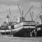
(a) Original

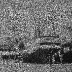
(b) Noisy

(c) Shan

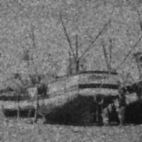
(d) Proposed

Figure 1: Image corrupted with speckle look L=1 and restored by different models.

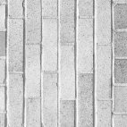
(a) Original

(b) Noisy

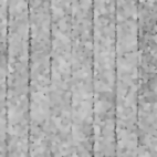
(c) Shan

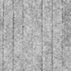
(d) Proposed

Figure 2: Image corrupted with speckle look L=1 and restored by different models.

(a) Original

(b) Noisy

(c) Shan

(d) Proposed

Figure 3: Image corrupted with speckle look L=3 and restored by different models.

(a) Original

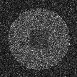
(b) Noisy

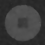
(c) Shan

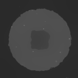
(d) Proposed

Figure 4: Image corrupted with speckle look L=1 and restored by different models.

(a) Original

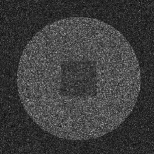
(b) Noisy

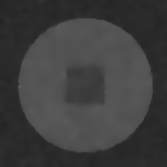
(c) Shan

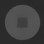
(d) Proposed

Figure 5: Image corrupted with speckle look L=3 and restored by different models.

(a) Original

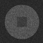
(b) Noisy

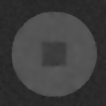
(c) Shan

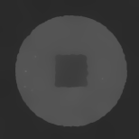
(d) Proposed

Figure 6: Image corrupted with speckle look L=5 and restored by different models.

(a) Original

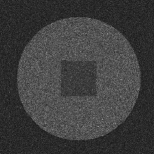
(b) Noisy

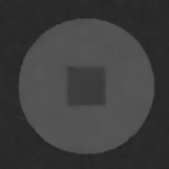
(c) Shan

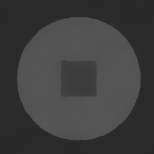
(d) Proposed

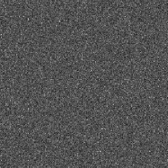
(e) Original

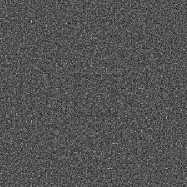
(f) Shan

(g) Proposed

Figure 7: Upper row: Image corrupted with speckle look L=10 and restored images. Lower row: Ratio images.

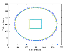
(a) Original

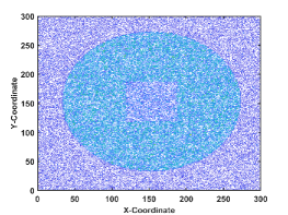
(b) Noisy

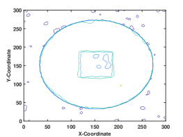
(c) Shan

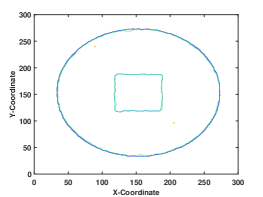
(d) Proposed

Figure 8: Contour maps of the restored imgaes in figure 7.

(a) Original

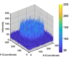
(b) Noisy

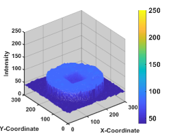
(c) Shan

(d) Proposed

Figure 9: 3D surface plots of the restored imgaes in figure 7.

Table 1: Left table: Comparison of SSIM and PSNR values of despeckled images. Right table: Parameter values for the numerical experiments.

Image $L$ Shan Model[44] Proposed Model SSIM PSNR SSIM PSNR Boat 1 0.5975 17.10 0.6096 17.12 3 0.7087 22.71 0.7347 22.85 5 0.7508 24.73 0.7905 24.93 10 0.8325 26.98 0.8422 27.12 33 0.8941 29.57 0.9057 29.72 Brick 1 0.2930 12.17 0.2954 12.19 3 0.3837 17.08 0.3861 17.11 5 0.4291 19.34 0.4355 19.40 10 0.4947 22.06 0.4960 22.18 33 0.5943 25.40 0.5961 25.53 Circle 1 0.9582 34.30 0.9644 34.70 3 0.9735 38.10 0.9772 39.53 5 0.9765 39.36 0.9806 40.73 10 0.9817 41.26 0.9865 42.85 33 0.9870 43.64 0.9889 44.62

Image $L$ Shan[44] Proposed $\alpha$ $\beta$ $\gamma$ $\nu$ $K$ Boat 1 1 1 5 1 2 3 1.2 1 4 1.5 2 5 1.3 1 2 1.5 1 10 1.4 1.2 2 2 1 33 1.5 1.5 2 3 1 Brick 1 1 1 5 1 4 3 1.2 1 4 1.3 3 5 1.4 1 2 1.5 2 10 1.6 1 2 2 1 33 1.7 1 2 3 1 Circle 1 1.5 2 10 1 1 3 1.5 2 10 1 1 5 2 2.25 5 1 1 10 2 2.25 2 1 1 33 2 2.5 2 1 1

6 Conclusion

This work suggests an efficient telegraph diffusion-based multiplicative speckle noise removal model. Such a new method intends to preserve the image edges during the noise removal process. To overcome the limitations of gradient-based despeckling models as well as parabolic PDE based models, we considered a hybrid approach. Here we combine a gray level indicator function with gradient-based diffusion in a telegraph diffusion framework for image restoration. To the best of our knowledge, the gray level indicator based telegraph diffusion model has not been used before for speckle noise suppression. Also, we established the existence and uniqueness of a weak solution to the suggested model using Schauder’s fixed point theorem. Moreover, we prove the boundedness of the weak solution. Numerical experiments have been conducted to highlight the efficiency of the proposed model for despeckling using different types of test images. Computational result of the present model compares with a recently developed model. From the experiment results of the proposed model, we can conclude that the images are suitably recovered without introducing undesired artifacts. A potential direction that the telegraph diffusion model can be extended to handle texture preservation issues in various real-life images, which are degraded by mixed noises. Another significant step might be the study of the advanced numerical solver to enhance the convergence speed of the proposed model.

References

• [1] Achim, A., Bezerianos, A., Tsakalides, P.: Novel bayesian multiscale method for speckle removal in medical ultrasound images. IEEE transactions on medical imaging 20(8), 772-783 (2001)
• [2] A. Averbuch, B. Epstein, N. Rabin, E. Turkel, Edge-enhancement postprocessing using artificial dissipation, IEEE transactions on image processing 15 (6) (2006) 1486-1498.
• [3] R. Adam, Sobolev spaces, in: Pure and Applied Mathematics Series of Monographs and Textbooks, Vol. 65, Academic Press, Inc., New York, San Francisco, London,, 1975.
• [4] Aiazzi, B., Alparone, L., Baronti, S.: Multiresolution local-statistics speckle filtering based on a ratio laplacian pyramid. IEEE Transactions on Geoscience and Remote Sensing 36(5), 1466-1476 (1998)
• [5] Alparone, L., Baronti, S., Carla, R.: Two-dimensional rank-conditioned median filter. IEEE Transactions on Circuits and Systems II: Analog and Digital Signal Processing 42(2), 130-132 (1995)
• [6] Alparone, L., Garzelli, A.: Decimated geometric filter for edge-preserving smoothing of non-white image noise. Pattern recognition letters 19(1), 89-96 (1998)
• [7] Argenti, F., Lapini, A., Bianchi, T., Alparone, L.: A tutorial on speckle reduction in synthetic aperture radar images. IEEE Geoscience and remote sensing magazine 1(3), 6-35 (2013)
• [8] Aubert, G., Aujol, J.F.: A variational approach to removing multiplicative noise. SIAM Journal on Applied Mathe- matics 68(4), 925-946 (2008)
• [9] Buades, A., Coll, B., Morel, J.M.: A non-local algorithm for image denoising. In: Computer Vision and Pattern Recognition, 2005. CVPR 2005. IEEE Computer Society Conference on, vol. 2, pp. 60-65. IEEE (2005)
• [10] Burckhardt, C.B.: Speckle in ultrasound b-mode scans. IEEE Transactions on Sonics and ultrasonics 25(1), 1-6 (1978)
• [11] Cao, Y., Yin, J., Liu, Q., Li, M.: A class of nonlinear parabolic-hyperbolic equations applied to image restoration. Nonlinear Analysis: Real World Applications 11(1), 253-261 (2010)
• [12] Chaira, T., Ray, A.: A new measure using intuitionistic fuzzy set theory and its application to edge detection. Applied soft computing 8(2), 919-927 (2008)
• [13] Coupé, P., Hellier, P., Kervrann, C., Barillot, C.: Bayesian non local means-based speckle filtering. In: Biomedical Imaging: From Nano to Macro, 2008. ISBI 2008. 5th IEEE International Symposium on, pp. 1291-1294. IEEE (2008)
• [14] Crimmins, T.R.: Geometric filter for speckle reduction. Applied optics 24(10), 1438-1443 (1985)
• [15] Deledalle, C.A., Denis, L., Tupin, F.: Iterative weighted maximum likelihood denoising with probabilistic patch-based weights. IEEE Transactions on Image Processing 18(12), 2661-2672 (2009)
• [16] Dong, G., Guo, Z., Wu, B.: A convex adaptive total variation model based on the gray level indicator for multiplicative noise removal. In: Abstract and Applied Analysis, vol. 2013. Hindawi Publishing Corporation (2013)
• [17] Dutt, V.: Statistical analysis of ultrasound echo envelope. Ultrasound Research Laboratory p. 181 (1995)
• [18] Evans, L.: Partial Differential Equations, in: Graduate Studies in Mathematics, vol. 19. American Mathematical Society, Providence, Rhode Island (1998)
• [19] Frost, V.S., Stiles, J.A., Shanmugan, K.S., Holtzman, J.C.: A model for radar images and its application to adaptive digital filtering of multiplicative noise. IEEE Transactions on pattern analysis and machine intelligence (2), 157-166 (1982)
• [20] Gonzalez, R.C., Woods, R.E.: Digital image processing (2002)
• [21] Hao, X., Gao, S., Gao, X.: A novel multiscale nonlinear thresholding method for ultrasonic speckle suppressing. IEEE Transactions on Medical Imaging 18(9), 787-794 (1999)
• [22] Hao, Y., Xu, J., Li, S., Zhang, X.: A variational model based on split bregman method for multiplicative noise removal. AEU-International Journal of Electronics and Communications 69(9), 1291-1296 (2015)
• [23] Huang, L.L., Xiao, L., Wei, Z.H.: Multiplicative noise removal via a novel variational model. EURASIP Journal on image and video processing 2010(1), 1 (2010)
• [24] Jain, S.K., Ray, R.K.: Edge detectors based telegraph total variational model for image filtering. In: Information Systems Design and Intelligent Applications, pp. 119-126. Springer (2016)
• [25] Jain, S.K., Ray, R.K.: Non-linear diffusion models for despeckling of images: achievements and future challenges. IETE Technical Review pp. 1-17 (2019)
• [26] Jain, S.K., Ray, R.K., Bhavsar, A.: Iterative solvers for image denoising with diffusion models: A comparative study. Computers $\&$ Mathematics with Applications 70(3), 191-211 (2015)
• [27] Jain, S.K., Ray, R.K., Bhavsar, A.: A nonlinear coupled diffusion system for image despeckling and application to ultrasound images. Circuits, Systems, and Signal Processing pp. 1-30 (2018)
• [28] Jidesh, P., Bini, A.: A complex diffusion driven approach for removing data-dependent multiplicative noise. In: Inter- national Conference on Pattern Recognition and Machine Intelligence, pp. 284-289. Springer (2013)
• [29] Jin, J.S.,Wang, Y., Hiller, J.: An adaptive nonlinear diffusion algorithm for filtering medical images. IEEE Transactions on Information Technology in Biomedicine 4(4), 298-305 (2000)
• [30] Jin, Z., Yang, X.: Analysis of a new variational model for multiplicative noise removal. Journal of Mathematical Analysis and Applications 362(2), 415-426 (2010)
• [31] Jin, Z., Yang, X.: A variational model to remove the multiplicative noise in ultrasound images. Journal of Mathematical Imaging and Vision 39(1), 62-74 (2011)
• [32] Kuan, D.T., Sawchuk, A.A., Strand, T.C., Chavel, P.: Adaptive noise smoothing lter for images with signal-dependent noise. IEEE Transactions on Pattern Analysis and Machine Intelligence (2), 165-177 (1985)
• [33] Lee, J.S.: Digital image enhancement and noise filtering by use of local statistics. IEEE transactions on pattern analysis and machine intelligence (2), 165-168 (1980)
• [34] J. L. Lions, Contrôle Optimal de Systèmes Gouvernés par des Équations aux Dérivées Partielles, Dunod, Paris, 1968.
• [35] Liu, M., Fan, Q.: A modified convex variational model for multiplicative noise removal. Journal of Visual Communi- cation and Image Representation 36, 187-198 (2016)
• [36] Liu, Q., Li, X., Gao, T.: A nondivergence p-laplace equation in a removing multiplicative noise model. Nonlinear Analysis: Real World Applications 14(5), 2046-2058 (2013)
• [37] Loizou, C.P., Pattichis, C.S., Christodoulou, C.I., Istepanian, R.S., Pantziaris, M., Nicolaides, A.: Comparative evalu- ation of despeckle filtering in ultrasound imaging of the carotid artery. IEEE transactions on ultrasonics, ferroelectrics, and frequency control 52(10), 1653-1669 (2005)
• [38] Majee, S., Jain, S.K., Ray, R.K., Majee, A.K.: A fuzzy edge detector driven telegraph total variation model for image despeckling, a preprint, arXiv https://128.84.21.199/abs/1908.01134 (2019)
• [39] Meer, P., Park, R.H., Cho, K.: Multiresolution adaptive image smoothing. CVGIP: Graphical Models and Image Processing 56(2), 140-148 (1994)
• [40] Perona, P., Malik, J.: Scale-space and edge detection using anisotropic diffusion. Pattern Analysis and Machine Intel- ligence, IEEE Transactions on 12(7), 629-639 (1990)
• [41] Prager, R., Gee, A., Treece, G., Berman, L.: Speckle detection in ultrasound images using first order statistics. University of Cambridge, Department of Engineering (2001)
• [42] Ratner, V., Zeevi, Y.Y.: Image enhancement using elastic manifolds. In: Image Analysis and Processing, 2007. ICIAP 2007. 14th International Conference on, pp. 769-774. IEEE (2007)
• [43] Rudin, L., Lions, P.L., Osher, S.: Multiplicative denoising and deblurring: Theory and algorithms. In: Geometric Level Set Methods in Imaging, Vision, and Graphics, pp. 103-119. Springer (2003)
• [44] Shan, X., Sun, J., Guo, Z.: Multiplicative noise removal based on the smooth diffusion equation. Journal of Mathe- matical Imaging and Vision pp. 1-17 (2019)
• [45] Shi, J., Osher, S.: A nonlinear inverse scale space method for a convex multiplicative noise model. SIAM Journal on Imaging Sciences 1(3), 294-321 (2008)
• [46] Sudha, S., Suresh, G., Sukanesh, R.: Speckle noise reduction in ultrasound images by wavelet thresholding based on weighted variance. International journal of computer theory and engineering 1(1), 7 (2009)
• [47] Sun, J., Yang, J., Sun, L.: A class of hyperbolic-parabolic coupled systems applied to image restoration. Boundary Value Problems 2016(1), 187 (2016)
• [48] A new similarity measure for nonlocal filtering in the presence of multiplicative noise. Compu- tational Statistics $\&$ Data Analysis 56(12), 3821-3842 (2012)
• [49] Wang, Z., Bovik, A.C., Sheikh, H.R., Simoncelli, E.P.: Image quality assessment: from error visibility to structural similarity. Image Processing, IEEE Transactions on 13(4), 600-612 (2004)
• [50] White, R.G.: A simulated annealing algorithm for sar and mti image cross-section estimation. In: Proc. SPIE, vol. 2316, pp. 137-145. vol (1994)
• [51] Yang, Y.Q., Zhang, C.Y.: Kernel based telegraph-diffusion equation for image noise removal. Mathematical Problems in Engineering 2014 (2014)
• [52] Yu, Y., Acton, S.T.: Speckle reducing anisotropic diffusion. IEEE Transactions on image processing 11(11), 1260-1270 (2002)
• [53] Zhang, F., Yoo, Y.M., Koh, L.M., Kim, Y.: Nonlinear diffusion in laplacian pyramid domain for ultrasonic speckle reduction. IEEE Transactions on Medical Imaging 26(2), 200-211 (2007)
• [54] Zhang, W., Li, J., Yang, Y.: Spatial fractional telegraph equation for image structure preserving denoising. Signal Processing 107, 368-377 (2015)
• [55] Zhou, Z., Guo, Z., Dong, G., Sun, J., Zhang, D., Wu, B.: A doubly degenerate diffusion model based on the gray level indicator for multiplicative noise removal. IEEE Transactions on Image Processing 24(1), 249-260 (2015)
• [56] Zhou, Z., Guo, Z., Zhang, D., Wu, B.: A nonlinear diffusion equation-based model for ultrasound speckle noise removal. Journal of Nonlinear Science 28(2), 443-470 (2018)