Social Optima in Robust Mean Field LQG Control: From Finite to Infinite Horizon

Abstract – This paper studies social optimal control of mean field LQG (linear-quadratic-Gaussian) models with uncertainty. Specially, the uncertainty is represented by a uncertain drift which is common for all agents. A robust optimization approach is applied by assuming all agents treat the uncertain drift as an adversarial player. In our model, both dynamics and costs of agents are coupled by mean field terms, and both finite- and infinite-time horizon cases are considered. By examining social functional variation and exploiting person-by-person optimality principle, we construct an auxiliary control problem for the generic agent via a class of forward-backward stochastic differential equation system. By solving the auxiliary problem and constructing consistent mean field approximation, a set of decentralized control strategies is designed and shown to be asymptotically optimal.

Index Terms – Linear quadratic optimal control, mean field control, model uncertainty, social functional variation, forward-backward stochastic differential equation.

I Introduction

I-A Background and Motivation

Mean field games and control have drawn increasing attention in many fields, including system control, applied mathematics and economics [4, 6, 10]. The mean field game involves a very large population of small interacting players with the feature that while the influence of each one is negligible, the impact of the overall population is significant. By now, mean field games and control have been intensively studied in the linear-quadratic-Gaussian (LQG) framework [16, 17, 22, 32, 27], and there is a large body of works on nonlinear models [19, 21, 7]. Huang et al. designed $\epsilon$-Nash equilibrium strategies for LQG mean field games with discount costs based on the proposed Nash certainty equivalence (NCE) approach [16, 17]. The NCE approach was then applied to the cases with long run average costs [22] and with Markov jump parameters [33], respectively. Lasry and Lions independently introduced the model of mean field games and studied the well-posedness problem of the limiting partial differential equations [21]. For further literature, readers are referred to [15, 33, 34] on mean field games with major players in continuous- or discrete-time, [7] on probabilistic analysis of mean field games, and [36] on the oblivious equilibrium in dynamic games.

Besides noncooperative games, social optima in mean field models have also drawn much attention. The social optimum control refers to that all the players cooperate to optimize the common social cost—the sum of individual costs, which is usually regarded as a type of team decision problem [11]. Huang et al. considered social optima in mean field LQG control, and provided an asymptotic team-optimal solution [18]. Wang and Zhang investigated a mean field social optimal problem where a Markov jump parameter appears as a common source of randomness [35]. Also, see [20] for social optima in mixed games, [2] for team-optimal control with finite population and partial information, and [24] for social optima of static mean field games.

Mathematical models can only be approximations of the real world. Actually, some parts of a model may be inexact. Thus, it is worthwhile to study the mean field control with model uncertainty [3]. The works [13, 14, 31] investigated the mean field games and control with a global uncertainty term. The “hard constraint” case (the disturbance is specified with a bound) was considered in [13] under which the substantial difficulty arises after the Lagrange multiplier is introduced. Authors in [14, 31] adopted the “soft constraint” approach ([3, 5, 8]) by removing the bound of the disturbance while the effort is penalized in the cost function. The works [30, 27] considered the case that each agent is paired with the local disturbance as an adversarial player, and provided an $\epsilon$-Nash equilibrium by tackling a Hamilton-Jacobi-Isaacs equation combined with a fixed-point analysis.

I-B Challenge and Contribution

This paper investigates mean field LQG social optimum control with a common uncertain drift, where both dynamics and costs of agents involve mean field coupled terms. To address the model uncertainty, a minus quadratic penalty term of drift is incorporated into the cost functional. There exist some substantial challenges in studying the problem. First, the socially optimal control with respect to drift uncertainty is a high-dimensional optimization problem with indefinite state weights. The corresponding convexity condition is very hard to verify. Second, by social variational derivation, the resulting limit system is governed by a controlled forward-backward stochastic differential equation (FBSDE). To design decentralized strategies, we need to solve the auxiliary optimal control problem subject to an FBSDE system. Meanwhile, the asymptotic optimality analysis is different from the general mean field LQG problems. Third, for the social optimum problem in the infinite horizon, we are faced with tackle infinite-horizon FBSDEs and the relevant optimal control problems.

In this paper, the social optimum control for the robust mean field LQG model is tackled by using stochastic maximum principle [38, 39, 40]. For the finite-horizon problem, we first obtain some low-dimensional convexity conditions and a set of FBSDEs by analyzing the variation of the centralized maximization cost to drift uncertainty. With the help of the Riccati equation, we further obtain a feedback type of the “worst-case” drift for the social optimum problem. Next, we construct an auxiliary optimal control problem based on the social variational derivation and the person-by-person optimality principle. By solving the auxiliary problem combined with consistent mean field approximations, a set of decentralized control laws is designed and further shown to be asymptotically robust social optimal by perturbation analysis. Finally, from asymptotic analysis to FBSDEs we design decentralized strategies and show their robust optimality for the infinite-horizon social optimum problem.

The main contributions of the paper are summarized as follows. (i) Social optimum control is studied for mean field models with a common uncertain drift, where coupled terms are included in both costs and dynamics of agents. By FBSDE and Riccati equation approaches we design a set of decentralized feedback control laws. (ii) By examining the social cost variation, we give low-dimensional convexity conditions and asymptotic convexity analysis for robust social optimum problems. (iii) From consistency requirements in mean field approximations, a system of differential equations is derived. The existence condition of solutions to consistency equations is characterized by a Riccati equation, instead of a fixed-point analysis. (iv) From the perturbation analysis to FBSDE, the decentralized strategies are shown to have asymptotic robust optimality. (v) By analyzing the asymptotic behavior of FBSDE, decentralized strategies for the infinite-horizon problem are designed and further shown be robust social optimal.

I-C Organization and Notation

The organization of the paper is as follows. In Section II, we consider the finite-horizon social optimization problem with drift uncertainty. By variational analysis, the centralized control with respect to drift uncertainty is obtained. Then an auxiliary optimal control problem is constructed based on person-by-person optimality. By solving this problem combined with consistent mean field approximations, a set of decentralized strategies is designed and further proved to be robust social optimal. Section III tackles the infinite-horizon social optimum problem. In Section IV, a numerical example is provided to verify the result. Section V concludes the paper.

Notation: Suppose that $(\Omega,\mathcal{F},\{\mathcal{F}_{t}\}_{0\leq t\leq T},\mathbb{P})$ is a complete filtered probability space. Throughout this paper, we denote by $\otimes$ the Kronecker product, $I_{m}$ m-dimensional identity matrix ($I_{n}$ abbreviated as $I$). We use $\|\cdot\|$ to denote the norm of a Euclidean space, or the Frobenius norm for matrices. For a symmetric matrix $Q$ and a vector $z$, $\|z\|_{Q}^{2}=z^{T}Qz$; for two vectors $x,y$, $\langle x,y\rangle=x^{T}y$. For a matrix (vector) $M$, $M^{T}$ denotes its transpose, $M>0$ means that $M$ is positive definite. Let $L^{2}_{\mathcal{F}}(0,T;\mathbb{R}^{k})$ denote the space of all $\mathbb{R}^{k}$-valued $\mathcal{F}_{t}$-progressively measurable processes $x(\cdot)$ satisfying $\mathbb{E}\int_{0}^{T}\|x(t)\|^{2}dt<\infty$, and $L^{2}_{\mathcal{F},\frac{\rho}{2}}(0,\infty;\mathbb{R}^{k})$ denote the space of all $\mathbb{R}^{k}$-valued $\mathcal{F}_{t}$-progressively measurable processes $x(\cdot)$ satisfying $\mathbb{E}\int_{0}^{\infty}e^{-\rho t}\|x(t)\|^{2}dt<\infty.$ $C([0,T],\mathbb{R}^{k})$ is the space of all $\mathbb{R}^{k}$-valued functions defined on $[0,T]$ which are continuous; $C_{\rho/2}([0,\infty),\mathbb{R}^{k})$ is a subspace of $C([0,\infty),\mathbb{R}^{k})$ which is given by $\{f|\int_{0}^{\infty}e^{-\rho t}\|f(t)\|^{2}dt<\infty\}.$ For convenience of presentation, we use $C$ (or $C_{1},C_{2},\ldots$) to denote a generic constant which may vary from place to place.

II Mean Field Social Control over a Finite Horizon

Consider a large population systems with $N$ agents. The $i$th agent evolves by the following stochastic differential equation:

$$dx_{i}(t)= [Ax_{i}(t)+Bu_{i}(t)+Gx^{(N)}(t)+f(t)]dt$$ (1)

$$+\sigma dW_{i}(t),\ 1\leq i\leq N,$$ (2)

where $x_{i}\in\mathbb{R}^{n}$ and $u_{i}\in\mathbb{R}^{r}$ are the state and the input of agent $i$, respectively. $x^{(N)}(t)=\frac{1}{N}\sum_{j=1}^{N}x_{j}(t)$. $\{W_{i},1\leq i\leq N\}$ are a sequence of mutually independent $d$-dimensional Brownian motions. $f\in L^{2}_{\mathcal{F}}(0,T;\mathbb{R}^{n})$ is an unknown disturbance, which reflects the effect imposed to each agent by the eternal environment. The cost function of agent $i$ is given by

$$J_{i}^{\rm F}(u)= \frac{1}{2}\mathbb{E}\int_{0}^{T}\Big{\{}\big{\|}x_{i}(t)-\Gamma x^{(N)}(t)-\eta\big{\|}^{2}_{Q}$$ (3)

$$+\|u_{i}(t)\|^{2}_{R_{1}}-\|f(t)\|^{2}_{R_{2}}\Big{\}}dt$$ (4)

$$+\frac{1}{2}\mathbb{E}\|x_{i}(T)\|^{2}_{H},$$ (5)

where $Q,R_{1},R_{2},H\in\mathbb{R}^{n\times n}$ are symmetric, $\Gamma\in\mathbb{R}^{n\times n}$ and $\eta\in\mathbb{R}^{n}$. $u=\{u_{1},\ldots,u_{N}\}$. Take $\{{\mathcal{F}}_{t}\}_{0\leq t\leq T}$ as the natural filtration generated by the $Nd$-dimensional Brownian motion $(W_{1},\cdots,W_{N})$. The decentralized control set is given by

$${\cal U}_{i}^{\rm F}=\Big{\{}u_{i}\ |\ u_{i}(t)\in\sigma(x_{i}(s),0\leq s\leq t),$$ (6)

$$\mathbb{E}\int_{0}^{T}\|u_{i}(t)\|^{2}dt<\infty\Big{\}}.$$

For comparison, define the centralized control set as

$${\cal U}_{c}^{\rm F}=\Big{\{}u_{i}| \ u_{i}(t)\in\sigma(x_{i}(0),W_{i}(s),0\leq s\leq t,\ 1\leq i\leq N),$$

$$\mathbb{E}\int_{0}^{T}\|u_{i}(t)\|^{2}dt<\infty\Big{\}}.$$

Denote $J_{\rm soc}^{\rm F}(u)=\sum_{i=1}^{N}J_{i}^{\rm F}(u)$. Let the social cost under the worst-case disturbance be

$$J_{\rm soc}^{\rm wo}({u})=\sup_{f\in{\mathcal{U}}_{c}^{\rm F}}J_{\rm soc}^{\rm F}({u},f).$$

Problem (PF): Seek a set of decentralized control laws $(\hat{u}_{1},\cdots,\hat{u}_{N})$ to minimize the social cost under the worst-case disturbance for System (1)-(3), i.e., $\inf_{u_{i}\in{\cal U}_{i}^{\rm F}}J_{\rm soc}^{\rm wo}({u})$.

Remark II.1

Different from [14, 30], we assume the disturbance $f$ is a common stochastic process. $f$ may stand for the impact from tax, subsidy or natural disaster. In this case, agents may be pessimistic to suppose the disturbance would use the information of all the agents to play against them.

We make the following assumptions.

(A0) $\{x_{i}(0)\}$ are independent random variables with the same mathematical expectation. $x_{i}(0)=x_{i0}$, $\mathbb{E}x_{i}(0)=\bar{x}_{0},1\leq i\leq N$. There exists a constant $C_{0}$ such that $\max_{1\leq i\leq N}\mathbb{E}\|x_{i0}\|^{2}<C_{0}$. Furthermore, $\{x_{i0},i=1,...,N\}$ and $\{W_{i},i=1,...,N\}$ are independent of each other.

(A1) $Q\geq 0$, $R_{1}>0$, $R_{2}>0$, and $H\geq 0$.

From now on, the time variable $t$ might be suppressed if necessary and no confusion occurs.

II-A The Control Problem with Respect to Model Uncertainty

Let $u_{i}=\check{u}_{i}\in{\cal U}_{c}^{\rm F},i=1,\cdots,N$ be fixed. The optimal control problem with respect to drift uncertainty is as follow:

$$\hbox{{(P1)} maximize}_{f\in{\mathcal{U}}_{c}^{\rm F}}J_{\rm soc}^{\rm F}(\check{u},f).$$

Clearly, (P1) is equivalent to the following problem:

$$\hbox{{(P1${}^{\prime}$)} minimize}_{f\in{\mathcal{U}}_{c}^{\rm F}}\check{J}_{\rm soc}^{\rm F}(f),$$

where

$$\check{J}_{\rm soc}^{\rm F}(f)= \frac{1}{2}\sum_{i=1}^{N}\mathbb{E}\int_{0}^{T}\Big{\{}-\big{\|}x_{i}-\Gamma x^{(N)}-\eta\big{\|}^{2}_{Q}+\|f\|^{2}_{R_{2}}\Big{\}}dt$$

$$-\frac{1}{2}\mathbb{E}\|x_{i}(T)\|^{2}_{H}.$$

Let $\textbf{x}=(x_{1}^{T},\cdots,x_{N}^{T})^{T}$, $\textbf{u}=(u_{1}^{T},\cdots,u_{N}^{T})^{T}$, $\textbf{1}=(1,\cdots,1)^{T}$, $\textbf{W}=(W_{1}^{T},\cdots,W_{N}^{T})^{T}$, $\textbf{A}=diag(A,\cdots,A)$, $\textbf{B}=diag(B,\cdots,B)$, ${\hat{\sigma}}=diag(\sigma,\cdots,\sigma)$, $\textbf{H}=diag(H,\cdots,H)$, $\hat{\textbf{Q}}=diag\{Q,\cdots,Q\}-\frac{1}{N}\textbf{11}^{T}\otimes\Psi,$ and $\hat{\bf{\eta}}=\textbf{1}\otimes\bar{\eta}$, where $\Psi\stackrel{{\scriptstyle\Delta}}{{=}}\Gamma^{T}Q+Q\Gamma-\Gamma^{T}Q\Gamma$ and $\bar{\eta}\stackrel{{\scriptstyle\Delta}}{{=}}Q\eta-\Gamma^{T}Q\eta$. We can write Problem (P1^′) as to minimize

$$\check{J}_{\rm soc}^{\rm F}(f)= \frac{1}{2}\mathbb{E}\int_{0}^{T}\Big{(}-\textbf{x}^{T}\hat{\textbf{Q}}\textbf{x}+2\hat{\bf{\eta}}^{T}\textbf{x}+{N}f^{T}R_{2}f\Big{)}dt$$

$$-\frac{1}{2}\mathbb{E}[\textbf{x}^{T}(T)\textbf{Hx}(T)],$$

subject to

$$d\textbf{x}(t)=\check{\textbf{A}}\textbf{x}(t)dt+\textbf{Bu}(t)dt+\textbf{1}\otimes f(t)dt+{\hat{\sigma}}d\textbf{W}(t).$$

where $\check{\textbf{A}}\stackrel{{\scriptstyle\Delta}}{{=}}{\textbf{A}}+\frac{1}{N}(\textbf{11}^{T}\otimes G).$

For the further existence analysis, we introduce the following assumptions:

(A2) Problem (P1^′) is convex in $f$;

(A2^′) Problem (P1^′) is uniformly convex in $f$.

Below are some necessary and sufficient conditions to ensure (A2) or (A2^′).

Proposition II.1

The following statements are equivalent:

(i) Problem (P1^′) is convex in $f$.

(ii) For any $f\in{\mathcal{U}}_{c}^{\rm F}$,

$$\int_{0}^{T}\Big{(}-\textbf{y}^{T}\hat{\textbf{Q}}\textbf{y}+{N}f^{T}R_{2}f\Big{)}dt-\|\textbf{y}(T)\|^{2}_{\textbf{H}}\geq 0,$$

where $\textbf{y}\in\mathbb{R}^{nN}$ satisfies

$$d\textbf{y}=(\check{\textbf{A}}\textbf{y}+\textbf{1}\otimes f)dt,\ \textbf{y}(0)=0.$$

(iii) For any $f\in{\mathcal{U}}_{c}^{\rm F}$,

$$\mathbb{E}\int_{0}^{T}\Big{\{}-\big{\|}(I-\Gamma)y_{i}\big{\|}^{2}_{Q}+\|f\|^{2}_{R_{2}}\Big{\}}dt-\|y_{i}(T)\|_{H}^{2}\geq 0,$$

where for $i=1$, 2, $\cdots$, $N$, $y_{i}$ satisfies

$$dy_{i}=[Ay_{i}+Gy^{(N)}+f]dt,\quad y_{i}(0)=0.$$ (7)

Proof. (i) $\Leftrightarrow$ (ii) is given in [14, 23]. From (7), we have $y_{1}=y_{2}=\cdots=y_{N}=y^{(N)}$. Thus,

$$\int_{0}^{T}\Big{(}-\textbf{y}^{T}\hat{\textbf{Q}}\textbf{y}+{N}f^{T}R_{2}f\Big{)}dt-\|\textbf{y}(T)\|^{2}_{\textbf{H}}$$ (8)

$$= \sum_{i=1}^{N}\!\!\int_{0}^{T}\!\!\Big{(}\!\!-\big{\|}y_{i}-\Gamma y_{i}\big{\|}^{2}_{Q}+\|f\|^{2}_{R_{2}}\Big{)}dt\!-\!\!\sum_{i=1}^{N}\!\|y_{i}(T)\|_{H}^{2}$$ (9)

$$= N\!\Big{[}\!\int_{0}^{T}\!\!\Big{(}\!\!-\big{\|}(I\!-\!\Gamma)y_{i}\big{\|}^{2}_{Q}\!+\!\|f\|^{2}_{R_{2}}\Big{)}dt\!-\!\|y_{i}(T)\|_{H}^{2}\Big{]},$$ (10)

which implies that (ii) is equivalent to (iii). $\hfill\Box$

Proposition II.2

The following statements are equivalent:

(i) Problem (P1^′) is uniformly convex in $f$.

(ii) There exists $\delta>0$ such that

$$\int_{0}^{T}\!\!\Big{(}\!-\textbf{y}^{T}\hat{\textbf{Q}}\textbf{y}+{N}f^{T}R_{2}f\Big{)}dt-\|\textbf{y}(T)\|^{2}_{\textbf{H}}\geq\delta\!\int_{0}^{T}\!\!\|f\|^{2}dt.$$

(iii) The equation

$$\dot{\textbf{P}}+\check{\textbf{A}}^{T}\textbf{P}+\textbf{P}\check{\textbf{A}}-\hat{\textbf{Q}}-\textbf{P}(\textbf{1}\otimes I)(NR_{2})^{-1}(\textbf{1}^{T}\otimes I)\textbf{P}=0,$$

with $\textbf{P}(T)=-\textbf{H}$ admits a solution in $C([0,T];\mathbb{R}^{nN})$.

(iv) The following equation admits a solution in $C([0,T];\mathbb{R}^{n})$,

$$\dot{P}+(A+G)^{T}P+P(A+G)-PR_{2}^{-1}P$$

$$-(I-\Gamma)^{T}Q(I-\Gamma)=0,\quad P(T)=-H.$$

(v) For any $t\in[0,T],$ $\det[(0,I)e^{\mathbb{A}t}(0,I)^{T}]>0,$ where

$$\mathbb{A}=\left(\begin{array}[]{cc}A+G+R^{-1}_{2}H&-R^{-1}_{2}\\[8.5359pt] \mathbb{A}_{21}&-(A+G+R^{-1}_{2}H)^{T}\end{array}\right)$$

with $\mathbb{A}_{21}=HR^{-1}_{2}H\!+\!(I\!-\!\Gamma)^{T}Q(I\!-\!\Gamma)\!+\!(A\!+\!G)^{T}H\!+\!H(A\!+\!G).$

Proof. (i)$\Leftrightarrow$(ii) is implied from [14, 23]. (i)$\Leftrightarrow$(iii) is given by Theorem 4.5 of [28]. By (8) and (ii), we have

$$\mathbb{E}\int_{0}^{T}\!\!\!\big{\{}-\|y_{i}\|^{2}_{Q(I-\Gamma)}+\|f\|^{2}_{R_{2}}\big{\}}dt-\|y_{i}(T)\|_{H}^{2}\geq\frac{\delta}{N}\mathbb{E}\int_{0}^{T}\!\!\|f\|^{2}dt.$$

By [28, Theorem 4.5], we obtain (ii)$\Leftrightarrow$(iv), which further implies (i)$\Leftrightarrow$(iv). (iv)$\Leftrightarrow$(v) is given by [14, 25]. $\hfill\Box$

By examining the variation of $\check{J}_{\rm soc}^{\rm F}$, we first obtain the necessary and sufficient conditions for the existence of centralized optimal control of (P1).

Theorem II.1

(P1^′) has a minimizer in ${\mathcal{U}}_{c}^{\rm F}$ if and only if (A2) holds and the following equation system admits a set of adapted solutions $(x_{i},p_{i},i=1,\cdots,N)$:

$$\left\{\begin{aligned} d\check{x}_{i}=&(A\check{x}_{i}+B\check{u}_{i}+{G}\check{x}^{(N)}\!-\!{R_{2}^{-1}}\check{p}_{j}^{(N)})dt\!+\!\sigma dW_{i},\\ d\check{p}_{i}=&-[A^{T}\check{p}_{i}+{G^{T}}\check{p}_{j}^{(N)}-Q\check{x}_{i}+{\Psi}\check{x}^{(N)}+\bar{\eta}]dt\cr&+\sum_{j=1}^{N}\beta_{i}^{j}dW_{j},\\ \check{x}_{i}(0)&={x_{i0}},\ \check{p}_{i}(T)=-H\check{x}_{i}(T),\ 1\leq i\leq N,\end{aligned}\right.$$ (12)

where $p^{(N)}=\frac{1}{N}\sum_{j=1}^{N}p_{j}$, and furthermore the minimizer is $\check{f}=-{R_{2}^{-1}}p^{(N)}$.

Proof. Suppose that $\check{f}=-R_{2}^{-1}p^{(N)}$, where $p_{i},i=1,\cdots,N$ are a set of solutions to the equation system

$$dp_{i}=\alpha_{i}dt+\beta_{i}^{i}dW_{i}+\sum_{j\not=i}\beta_{i}^{j}dW_{j},\ p_{i}(T)=-Hx_{i}(T),$$ (13)

where $i=1$, $\cdots$, $N$; $\alpha_{i}$ and $\beta_{i}^{j}$ are to be determined. Denote by $\check{x}_{i}$ the state of agent $i$ under the control $\check{u}_{i}$ and the drift $\check{f}$. For any $f\in{\mathcal{U}}_{c}^{\rm F}$ and $\varepsilon\in\mathbb{R}$, let $f^{\varepsilon}=\check{f}+\varepsilon f$. Let $x_{i}^{\varepsilon}$ be the solution of the following perturbed state equation

$$dx_{i}^{\varepsilon}=\big{(}Ax_{i}^{\varepsilon}+B\check{u}_{i}+\check{f}+\varepsilon f+\frac{G}{N}\sum_{i=1}^{N}x^{\varepsilon}_{i}\big{)}dt+\sigma dW_{i},$$

with $x_{i}^{\varepsilon}(0)=x_{i0}$, $i=1$, 2, $\cdots$, $N$.

Let $y_{i}=(x_{i}^{\varepsilon}-\check{x}_{i})/\varepsilon$, and $y^{(N)}=\sum_{i=1}^{N}y_{i}/{N}$. It can be verified that ${y}_{i}$ satisfies (7). Then, by Itô’s formula,

$$-\mathbb{E}\langle H\check{x}_{i}(T),y_{i}(T)\rangle$$ (14)

$$= \mathbb{E}[\langle p_{i}(T),y_{i}(T)\rangle-\langle p_{i}(0),y_{i}(0)\rangle]$$ (15)

$$= \mathbb{E}\int_{0}^{T}\big{[}\langle\alpha_{i},y_{i}\rangle+\langle p_{i},Ay_{i}+Gy^{(N)}+f\rangle\big{]}dt.$$ (16)

We have

$$\check{J}_{\rm soc}^{\rm F}(\check{f}+\varepsilon f)-\check{J}_{\rm soc}^{\rm F}(\check{f})=\varepsilon\Lambda_{1}+\frac{\varepsilon^{2}}{2}\Lambda_{2}$$ (17)

where

$$\Lambda_{1}\stackrel{{\scriptstyle\Delta}}{{=}} \sum_{i=1}^{N}\mathbb{E}\int_{0}^{T}\!\!\Big{[}\big{\langle}\!\!-\!Q\big{(}\check{x}_{i}\!-\!(\Gamma\check{x}^{(N)}\!+\!\eta)\big{)},y_{i}\!-\!\Gamma y^{(N)}\big{\rangle}$$

$$+\langle R_{2}\check{f},f\rangle\Big{]}dt-\sum_{i=1}^{N}\mathbb{E}\langle H\check{x}_{i}(T),y_{i}(T)\rangle,$$

$$\Lambda_{2}\stackrel{{\scriptstyle\Delta}}{{=}} \sum_{i=1}^{N}\mathbb{E}\int_{0}^{T}\Big{\{}-\big{\|}y_{i}-\Gamma y^{(N)}\big{\|}^{2}_{Q}+\|f\|^{2}_{R_{2}}\Big{\}}dt.$$

Note that

$$\sum_{i=1}^{N}\mathbb{E}\int_{0}^{T}\big{\langle}-Q\big{(}\check{x}_{i}-(\Gamma\check{x}^{(N)}+\eta)\big{)},\Gamma y^{(N)}\big{\rangle}dt$$

$$= \mathbb{E}\int_{0}^{T}\!\!\big{\langle}\!-\!\Gamma^{T}Q\sum_{i=1}^{N}\big{(}\check{x}_{i}-(\Gamma\check{x}^{(N)}+\eta)\big{)},\frac{1}{N}\sum_{j=1}^{N}y_{j}\big{\rangle}dt$$

$$= \sum_{j=1}^{N}\mathbb{E}\int_{0}^{T}\!\!\big{\langle}-\frac{\Gamma^{T}Q}{N}\sum_{i=1}^{N}\big{(}\check{x}_{i}-(\Gamma\check{x}^{(N)}+\eta)\big{)},y_{j}\big{\rangle}dt$$

$$= \sum_{j=1}^{N}\mathbb{E}\int_{0}^{T}\!\!\big{\langle}-{\Gamma^{T}Q}\big{(}(I-\Gamma)\check{x}^{(N)}-\eta\big{)},y_{j}\big{\rangle}dt.$$

From (14), one can obtain that

$$\Lambda_{1}= \mathbb{E}\sum_{i=1}^{N}\int_{0}^{T}\Big{[}\big{\langle}-Q\big{(}\check{x}_{i}-(\Gamma\check{x}^{(N)}+\eta)\big{)},$$

$$y_{i}-\Gamma y^{(N)}\big{\rangle}+\langle R_{2}\check{f},f\rangle\Big{]}dt$$

$$+ \sum_{i=1}^{N}\mathbb{E}\int_{0}^{T}\big{[}\langle\alpha_{i},y_{i}\rangle+\langle p_{i},Ay_{i}+Gy^{(N)}+f\rangle\big{]}dt$$

$$= \mathbb{E}\int_{0}^{T}\Big{\langle}NR_{2}\check{f}+\sum_{i=1}^{N}p_{i},f\Big{\rangle}dt$$

$$+ \sum_{i=1}^{N}\mathbb{E}\int_{0}^{T}\Big{\langle}-Q\big{(}\check{x}_{i}-(\Gamma\check{x}^{(N)}+\eta)\big{)}+A^{T}p_{i}$$

$$+ {\Gamma^{T}Q}\big{(}(I-\Gamma)\check{x}^{(N)}-\eta\big{)}+\alpha_{i}+{G^{T}}p^{(N)},y_{i}\Big{\rangle}dt,$$

From (17), $\check{f}$ is a minimizer to Problem (P1^′) if and only if $\Lambda_{2}\geq 0$ and $\Lambda_{1}=0$. By Proposition II.1, $\Lambda_{2}\geq 0$ if and only if (A2) holds. $\Lambda_{1}=0$ is equivalent to

$$\alpha_{i}= -\big{[}A^{T}p_{i}+{G^{T}}p^{(N)}+\Gamma^{T}Q\big{(}(I-\Gamma)\check{x}^{(N)}-\eta\big{)}$$

$$-Q\big{(}\check{x}_{i}-(\Gamma\check{x}^{(N)}+\eta))\big{]},$$

$$\check{f}= -{R_{2}^{-1}}p^{(N)}.$$

Thus, we have the optimality system (12). Namely, $\Lambda_{1}=0$ if and only if (12) admits a solution $(\check{x}_{i},\check{p}_{i},i=1,\cdots,N)$. $\Box$

Let $\check{u}^{(N)}=\frac{1}{N}\sum_{i=1}^{N}\check{u}_{i}$, and $\check{p}^{(N)}=\frac{1}{N}\sum_{i=1}^{N}\check{p}_{i}$. It follows from (12) that

$$\left\{\begin{aligned} d\check{x}^{(N)}=&\big{(}(A+G)\check{x}^{(N)}+B\check{u}^{(N)}-R_{2}^{-1}\check{p}^{(N)}\big{)}dt\\ &+\frac{1}{N}\sum_{i=1}^{N}\sigma dW_{i},\\ d\check{p}^{(N)}=&-\!\Big{[}(A+G)^{T}\check{p}^{(N)}+(\Psi-Q)\check{x}^{(N)}+\bar{\eta}\Big{]}dt\\ &+\frac{1}{N}\sum_{i=1}^{N}\sum_{j=1}^{N}{\beta}_{i}^{j}dW_{j},\\ \check{x}^{(N)}(0)&=\frac{1}{N}\sum_{i=1}^{N}x_{i0},\ \check{p}^{(N)}(T)=-H\check{x}^{(N)}(T).\end{aligned}\right.$$ (18)

Proposition II.3

The FBSDE (12) admits a set of adapted solutions $(x_{i},p_{i},i=1,\cdots,N)$ if and only if (18) admits an adapted solution $(x^{(N)},p^{(N)})$.

Proof. If (18) admits an adapted solution $(x^{(N)},p^{(N)})$, then (12) is decoupled. The existence of a set of solutions to (12) follows. The part of necessity is straightforward. $\Box$

We further discuss the optimal feedback control of (P1^′). Let $\check{p}^{(N)}(t)=P(t)\check{x}^{(N)}(t)+\check{s}(t)$, $t\geq 0$, where $P\in\mathbb{R}^{n\times n}$ and $\check{s}\in\mathbb{R}^{n}$. Then by (18) we have

$$d\check{p}^{(N)}= P\Big{[}(A+G)\check{x}^{(N)}+B\check{u}^{(N)}-R_{2}^{-1}\check{p}^{(N)})dt$$

$$+\frac{1}{N}\sum_{i=1}^{N}\sigma dW_{i}\Big{]}+\dot{P}\check{x}^{(N)}dt+d\check{s}$$

$$= -\Big{[}(A+G)^{T}(P\check{x}^{(N)}+\check{s})+(\Psi-Q)\check{x}^{(N)}$$

$$+\bar{\eta}\Big{]}dt+\frac{1}{N}\sum_{i=1}^{N}\sum_{j=1}^{N}{\beta}_{i}^{j}dW_{j}.$$

This implies

$$\dot{P}+(A+G)^{T}P+P(A+G)-PR_{2}^{-1}P$$ (19)

$$-(I-\Gamma)^{T}Q(I-\Gamma)=0,\ P(T)=-H,$$ (20)

$$d\check{s}+\big{[}(A+\bar{G})^{T}\check{s}+PB\check{u}^{(N)}+\bar{\eta}\big{]}dt$$ (21)

$$+\frac{1}{N}\sum_{i=1}^{N}\sum_{j=1}^{N}\big{(}\frac{\sigma}{N}-\beta_{i}^{j}\big{)}dW_{j}=0,\ \check{s}(T)=0,$$ (22)

where $\bar{G}\stackrel{{\scriptstyle\Delta}}{{=}}G-R_{2}^{-1}P$.

By the local Lipschitz continuous property of the quadratic (matrix) function, (19) must admit a unique local solution in a small time duration $[T_{0},T]$. The global existence of the solution for $t\in[-\infty,T]$ or $[0,T]$ can be referred to [9, 1]. From Proposition II.2, we obtain that under (A2^′), (19) has a unique solution in $C([0,T],\mathbb{R}^{n\times n})$.

Theorem II.2

Under (A0), (A1), (A2^′), Problem (P1^′) has a minimizer

$$\check{f}(t)=-{R_{2}^{-1}}[P(t)\check{x}^{(N)}(t)+\check{s}(t)],\ t\geq 0,$$ (23)

where $P$ and $\check{s}$ are solutions of (19) and (21), respectively.

Proof. Under (A2^′), (19) admits a unique solution $P$, which implies (21) has a unique solution $\check{s}$ in $C([0,T],\mathbb{R}^{n})$. By [25, Theorem 2.4.1], (18) admits a unique solution $(\check{x}^{(N)},\check{p}^{(N)}),$ where $\check{p}^{(N)}=P\check{x}^{(N)}+\check{s}$. From Proposition II.3, (12) is solvable. This with Theorem II.1 completes the proof. $\Box$

Remark II.2

From the above analysis, (A2^′) is sufficient for solvability of FBSDE (12). Indeed, from [25], (A2^′) is also a necessary condition to ensure that the solvability of (12) holds for any $\check{u}_{i}\in{\mathcal{U}}_{c}^{\rm F}$.

II-B Distributed Strategy Design

After the “worst-case” drift $\check{f}$ is applied, we have the following optimal control problem.

(P2): Minimize ${J}_{\rm soc}^{\rm F}(u,\check{f}(u))$ over $\{u_{i}\in{\mathcal{U}}_{c}^{\rm F},i=1,\cdots,N\}$, where

$$dx_{i}= [Ax_{i}+Bu_{i}+Gx^{(N)}\!-\!{R_{2}^{-1}}(Px^{(N)}+s)]dt$$ (24)

$$+\sigma dW_{i},\ 1\leq i\leq N,$$ (25)

$$ds= -\big{[}(A+\bar{G})^{T}s+PB{u}^{(N)}+\bar{\eta}\big{]}dt$$ (26)

$$+\frac{1}{N}\sum_{i=1}^{N}\sum_{j=1}^{N}(\beta_{i}^{j}-\frac{\sigma}{N})dW_{j},s(T)=0.$$ (27)

$${J}_{\rm soc}^{\rm F}(u)= \frac{1}{2}\sum_{i=1}^{N}\mathbb{E}\int_{0}^{T}\Big{\{}\big{\|}x_{i}-\Gamma x^{(N)}-\eta\big{\|}^{2}_{Q}+\|u_{i}\|^{2}_{R_{1}}$$ (28)

$$\!-\!\|Px^{(N)}+s\|^{2}_{R_{2}^{-1}}\Big{\}}dt\!+\!\frac{1}{2}\mathbb{E}\|x_{i}(T)\|_{H}^{2}.$$ (29)

We first show that Problem (P2) has the property of uniformly convexity under certain conditions.

Lemma II.1

Assume that A0), A1), A2^′) hold. There exists a sufficiently large $C_{0}>0$ with $R_{1}>C_{0}I$ and $R_{2}>C_{0}I$ such that Problem (P2) is uniformly convex in u.

Proof. Denote ${\bf{\bar{Q}}}=diag\{Q,\cdots,Q\}-\frac{1}{N}\textbf{11}^{T}\otimes(\Psi+PR_{2}^{-1}P)$, $\textbf{R}_{1}=diag\{R_{1},\cdots,R_{1}\}$, ${\bf{\bar{A}}}=diag\{A,\cdots,A\}+\frac{1}{N}\textbf{11}^{T}\otimes(G-R_{2}^{-1}P)$. By a similar argument with [23], we obtain that Problem (P2) is uniformly convex if for any $u_{i}\in{\mathcal{U}}_{c}^{\rm F}$,

$$\mathbb{E}\int_{0}^{T}\Big{(}\textbf{z}^{T}{\bf{\bar{Q}}}\textbf{z}+\textbf{u}^{T}\textbf{R}_{1}\textbf{u}-N\grave{s}^{T}R_{2}^{-1}\grave{{s}}\Big{)}dt$$

$$+\mathbb{E}\|\textbf{z}(T)\|_{\bf{H}}^{2}\geq\delta\mathbb{E}\int_{0}^{T}\|\textbf{u}\|^{2}dt$$

where $\textbf{z}\in\mathbb{R}^{nN}$ and $\grave{s}\in\mathbb{R}^{n}$ satisfy

$$d\textbf{z}= (\bar{\textbf{A}}\textbf{z}+\textbf{B}\textbf{u}-\textbf{1}\otimes R_{2}^{-1}\grave{s})dt,\ \textbf{z}(0)=0,$$ (30)

$$d\grave{s}= -\big{[}(A+\bar{G})^{T}\grave{s}+\frac{1}{N}PB(\textbf{1}^{T}\otimes I)\textbf{u}\big{]}dt$$ (31)

$$+\frac{1}{N}\sum_{i=1}^{N}\sum_{j=1}^{N}\grave{\beta}_{i}^{j}dW_{j},\ \grave{s}(T)=0.$$ (32)

By [38, Chapter 7] and (31),

$$\mathbb{E}\int_{0}^{T}\|\grave{s}(t)\|^{2}dt\leq\frac{C_{1}}{N^{2}}\mathbb{E}\int_{0}^{T}\|\textbf{1}^{T}\otimes I\|^{2}\|\textbf{u}(t)\|^{2}dt$$ (33)

$$\leq \frac{C_{1}}{N}\mathbb{E}\int_{0}^{T}\|\textbf{u}(t)\|^{2}dt.$$ (34)

This with (30) leads to $\mathbb{E}\int_{0}^{T}\|\textbf{z}\|^{2}dt\leq C_{2}\int_{0}^{T}\mathbb{E}\|\textbf{u}\|^{2}dt$. Note that

$$\lambda_{min}({\bf{\bar{Q}}})\geq \lambda_{min}(Q)\!-[\lambda_{max}(\Psi)\!+\!\lambda_{max}(PR_{2}^{-1}P)]$$

$$\geq -[\lambda_{max}(\Psi)+\lambda_{max}(PR_{2}^{-1}P)],$$

where $\lambda_{min}(Q)$ and $\lambda_{max}(Q)$ are smallest and largest eigenvalues of $Q$, respectively. From this with (33), there exists $\delta>0$ and $C_{0}>0$ such that for $R_{1}>C_{0}I$ and $R_{2}>C_{0}I$,

$$\mathbb{E}\int_{0}^{T}\Big{(}\textbf{z}^{T}{\bf{\bar{Q}}}\textbf{z}\!+\!\textbf{u}^{T}\textbf{R}_{1}\textbf{u}-N\grave{s}^{T}R_{2}^{-1}\grave{{s}}\Big{)}dt+\mathbb{E}\|\textbf{z}(T)\|_{\bf{H}}^{2}$$

$$\geq\mathbb{E}\int_{0}^{T}\Big{[}\textbf{u}^{T}(\textbf{R}_{1}-{C}_{0}I_{nN})\textbf{u}\Big{]}dt\geq\delta\mathbb{E}\int_{0}^{T}(\textbf{u}^{T}\textbf{u})dt.$$

$\Box$

II-B1 The Social Variational Derivation

Note that the social optimum implies the person-by-person optimality [11]. If the social cost is convex, then the socially optimal solution exists and coincides with the person-by-person optimal solution [35]. We now provide a transformation of the original social optimum problem by variational derivation and person-by-person optimality. Suppose that $\hat{u}=(\hat{u}_{1},\cdots,\hat{u}_{N})$ is a minimizer to Problem (P2), where $\hat{u}_{j}\in{\mathcal{U}}_{c}^{\rm F}$. Let $\hat{x}_{j}$ correspond to $\hat{u}_{j}$, $j=1,\cdots,N$ and $\hat{x}^{(N)}=\frac{1}{N}\sum_{j=1}^{N}\hat{x}_{j}$. Let $\hat{s}$ correspond to $\hat{u}_{1}$, $\cdots$, $\hat{u}_{N}$. Fix $\hat{u}_{-i}=(\hat{u}_{1},\cdots,\hat{u}_{i-1},\hat{u}_{i+1},\cdots,\hat{u}_{N})$, and perturb $u_{i}$. Denote $\delta u_{i}=u_{i}-\hat{u}_{i}$, $\delta x_{j}=x_{j}-\hat{x}_{j}$, $\delta x^{(N)}=\frac{1}{N}\sum_{j=1}^{N}\delta x_{j}$ and $\delta s=s-\hat{s}$. Let the strategy variation $\delta{u}_{i}$ be adapted to ${\mathcal{F}}_{t}$ and satisfy $\mathbb{E}\int_{0}^{T}\|\delta{u}_{i}\|^{2}dt<\infty.$ Let $\delta{J}_{i}$ be the variation of ${J}_{i}$ with respect to $\delta u_{i}$. By (24) and (26),

$$\frac{d\delta x_{j}}{dt}= A\delta x_{j}+\frac{\bar{G}}{N}\delta x_{i}+\frac{\bar{G}}{N}\sum_{k\not=i}\delta x_{k}-R_{2}^{-1}\delta s,$$ (35)

$$\ j\not=i,\ \delta x_{j}(0)=0,$$ (36)

$$d\delta s= -\big{[}(A+\bar{G})^{T}\delta s+\frac{1}{N}PB\delta u_{i}\big{]}dt$$ (37)

$$+\frac{1}{N}\sum_{i=1}^{N}\sum_{j=1}^{N}\delta\beta_{i}^{j}dW_{j},\ \delta s(T)=0.$$ (38)

where $\bar{G}\stackrel{{\scriptstyle\Delta}}{{=}}G-R_{2}^{-1}P$. This implies $\delta x_{j}=\delta x_{k}$, for any $j,k\not=i$. Thus,

$$\frac{d\delta x_{j}}{dt}\!=\!(A+\frac{N-1}{N}\bar{G})\delta x_{j}+\frac{\bar{G}}{N}\delta x_{i}\!-\!R_{2}^{-1}\delta s,\delta x_{j}(0)\!=\!0,$$

which gives that

$$\delta x_{j}(t)\!=\!\!\int_{0}^{t}\!\!e^{(A+\frac{N-1}{N}\bar{G})(t-\tau)}\big{(}\frac{\bar{G}}{N}\delta x_{i}(\tau)-R_{2}^{-1}\delta s(\tau)\big{)}d\tau\!.$$

We further have

$$\delta x^{(N)}(t)= \frac{1}{N}\delta x_{i}(t)+\frac{N-1}{N}\int_{0}^{t}e^{(A+\frac{N-1}{N}\bar{G})(t-\tau)}$$

$$\times\Big{(}\frac{\bar{G}}{N}\delta x_{i}(\tau)-R_{2}^{-1}\delta s(\tau)\Big{)}d\tau.$$

By this with (26), one can obtain

$$\delta J_{i}(u,\check{f})= \mathbb{E}\int_{0}^{T}\Big{\{}[\hat{x}_{i}-\Gamma\hat{x}^{(N)}-\eta]^{T}Q\big{[}\delta x_{i}-{\Gamma}\delta x^{(N)}\big{]}$$

$$-(P\hat{x}^{(N)}+s)^{T}R_{2}^{-1}(P\delta x^{(N)}+\delta s)$$

$$+\hat{u}_{i}^{T}R_{1}\delta u_{i}\Big{\}}dt+\mathbb{E}[x_{i}^{T}(T)H\delta x_{i}(T)],$$

and for $j\not=i$,

$$\delta J_{j}(u,\check{f})$$

$$= \mathbb{E}\int_{0}^{T}\big{[}(\hat{x}_{j}-\Gamma\hat{x}^{(N)}-\eta)^{T}Q(\delta x_{j}-\Gamma\delta x^{(N)})$$

$$-(P\hat{x}^{(N)}+s)^{T}R_{2}^{-1}(P\delta x^{(N)}+\delta s)\big{]}dt$$

$$+\mathbb{E}[x_{j}^{T}(T)H\delta x_{j}(T)].$$

The above equation further implies that

$$\sum_{j\not=i}\delta J_{j}(u,\check{f})$$

$$= \mathbb{E}\int_{0}^{T}\big{(}\hat{x}_{-i}^{(N)}-\textstyle{\frac{N-1}{N}}(\Gamma\hat{x}^{(N)}+\eta)\big{)}^{T}Q\Big{[}(I-\textstyle{\frac{N-1}{N}}\Gamma)$$

$$\cdot\int_{0}^{t}e^{(A+\frac{N-1}{N}\bar{G})(t-\tau)}(\bar{G}\delta x_{i}-NR_{2}^{-1}\delta s)d\tau-{\Gamma}\delta x_{i}\Big{]}$$

$$-(P\hat{x}^{(N)}+s)^{T}R_{2}^{-1}\Big{[}P\big{(}\textstyle{\frac{(N-1)^{2}}{N^{2}}}\int_{0}^{t}e^{(A\!+\!\frac{N-1}{N}\bar{G})(t-s)}$$

$$\cdot\bar{G}\delta x_{i}ds\!+\!\textstyle{\frac{N-1}{N}}\delta x_{i}\big{)}\!+\!(N-1)\delta s\Big{]}dt+\mathbb{E}\Big{[}x_{-i}^{(N)}(T)^{T}$$

$$\cdot H\int_{0}^{T}e^{(A+\frac{N-1}{N}\bar{G})(T-t)}(\bar{G}\delta x_{i}-NR_{2}^{-1}\delta s)dt\Big{]},$$

where $\hat{x}_{-i}^{(N)}=\frac{1}{N}\sum_{j\not=i}\hat{x}_{j}$. Let $\delta\psi_{i}=N\delta s$. Then from (38),

$$d\delta\psi_{i}= -\big{[}(A+\bar{G})^{T}\delta\psi_{i}+PB\delta u_{i}\big{]}dt$$ (39)

$$+\sum_{i=1}^{N}\sum_{j=1}^{N}\delta\beta_{i}^{j}dW_{j},\delta\psi_{i}(T)=0.$$ (40)

For large $N$, it is plausible to approximate $\hat{x}^{(N)}$ by a deterministic function $\bar{x}$. The zero first-order variational condition combined with the mean field approximation gives

$$\mathbb{E}\int_{0}^{T}\Big{\{}(\hat{x}_{i}-\Gamma\bar{x}-\eta)^{T}Q\delta x_{i}-\big{[}((I-\Gamma)\bar{x}-\eta)^{T}Q\Gamma$$ (41)

$$+(P\bar{x}+\bar{s})^{T}R_{2}^{-1}P\big{]}\delta x_{i}+\big{[}((I-\Gamma)\bar{x}-\eta)^{T}Q(I-\Gamma)$$ (42)

$$\!-\!(P\bar{x}\!+\!\bar{s})^{T}R_{2}^{-1}P\big{]}\!\!\int_{0}^{t}e^{(A+\bar{G})(t-\tau)}(\bar{G}\delta x_{i}\!-\!R_{2}^{-1}\delta\psi_{i})d\tau$$ (43)

$$-(P\bar{x}+\bar{s})^{T}R_{2}^{-1}\delta\psi_{i}+\hat{u}_{i}^{T}R_{1}\delta u_{i}$$ (44)

$$+\bar{x}^{T}(T)He^{(A+\bar{G})(T-t)}(\bar{G}\delta x_{i}-R_{2}^{-1}\delta\psi_{i})\Big{\}}dt$$ (45)

$$+\mathbb{E}[x_{i}^{T}(T)H\delta x_{i}(T)]=0,$$ (46)

where $\bar{x}\in C([0,T],\mathbb{R}^{n})$ is an approximation of $\hat{x}^{(N)}$. From observation, the equation (41) is the zero variation condition for the optimal control problem with the cost function:

$$J_{i}^{\prime}(u_{i})$$ (47)

$$= \frac{1}{2}\mathbb{E}\int_{0}^{T}\Big{\{}x^{T}_{i}Qx_{i}+2\big{[}-\left((I-\Gamma)\bar{x}-\eta\right)^{T}Q\Gamma$$ (48)

$$-(\Gamma\bar{x}+\eta)^{T}Q-(P\bar{x}+\bar{s})^{T}R_{2}^{-1}P\big{]}x_{i}$$ (49)

$$+2\big{[}((I-\Gamma)\bar{x}-\eta)^{T}Q(I-\Gamma)-(P\bar{x}+\bar{s})^{T}R_{2}^{-1}P\big{]}$$ (50)

$$\times\int_{0}^{t}e^{(A+\bar{G})(t-\tau)}(\bar{G}x_{i}-R_{2}^{-1}\psi_{i})d\tau$$ (51)

$$+\bar{x}^{T}(T)He^{(A+\bar{G})(T-t)}(\bar{G}x_{i}-R_{2}^{-1}\psi_{i})$$ (52)

$$+{u}_{i}^{T}R_{1}u_{i}\Big{\}}dt+\frac{1}{2}\mathbb{E}[x_{i}^{T}(T)Hx_{i}(T)]$$ (53)

$$= \frac{1}{2}\mathbb{E}\int_{0}^{T}\!\!\Big{\{}x_{i}^{T}Qx_{i}-2\big{[}\Psi\bar{x}+\bar{\eta}+(P\bar{x}+\bar{s})^{T}R_{2}^{-1}P\big{]}x_{i}$$ (54)

$$+2v^{T}(\bar{G}x_{i}-R_{2}^{-1}\psi_{i})+u_{i}^{T}R_{1}u_{i}\Big{\}}dt$$ (55)

$$+\frac{1}{2}\mathbb{E}[x_{i}^{T}(T)Hx_{i}(T)],$$ (56)

where the second equality holds by an exchange of order of the integration, and

$$v(t)\stackrel{{\scriptstyle\Delta}}{{=}} \int_{t}^{T}e^{({A+\bar{G}})^{T}(\tau-t)}\big{[}(I-\Gamma)^{T}Q((I-\Gamma)\bar{x}-\eta)$$

$$-PR_{2}^{-1}(P\bar{x}+\bar{s})\big{]}d\tau+e^{(A+\bar{G})^{T}(T-t)}H\bar{x}(T).$$

II-B2 Mean field approximation

Based on (24), (39) and (47), we construct the following auxiliary optimal control problem.

(P3): minimize $\bar{J}_{i}(u_{i})$ over $u_{i}\in{\cal U}_{i}$, where

$$d\grave{x}_{i}= [A\grave{x}_{i}+Bu_{i}+G\bar{x}-{R_{2}^{-1}}(P\bar{x}+\bar{s})]dt$$ (57)

$$+\sigma dW_{i},\ \grave{x}_{i}(0)=x_{i0},$$ (58)

$$d\psi_{i}= -\big{[}(A+\bar{G})^{T}\psi_{i}+PBu_{i}\big{]}dt$$ (59)

$$+z_{i}^{i}dW_{i},\ \psi_{i}(T)=0.$$ (60)

$$\bar{J}_{i}(u_{i})= \frac{1}{2}\mathbb{E}\int_{0}^{T}\Big{[}\grave{x}_{i}^{T}Q\grave{x}_{i}-2(P\bar{x}+\bar{s})^{T}R_{2}^{-1}P\grave{x}_{i}$$ (61)

$$-2(\Psi\bar{x}+\bar{\eta})^{T}\grave{x}_{i}+2v^{T}(\bar{G}\grave{x}_{i}-R_{2}^{-1}\psi_{i})$$ (62)

$$-2(P\bar{x}+\bar{s})^{T}R_{2}^{-1}\psi_{i}+u_{i}^{T}R_{1}u_{i}\Big{]}dt$$ (63)

$$+\frac{1}{2}\mathbb{E}[\grave{x}_{i}^{T}(T)H\grave{x}_{i}(T)].$$ (64)

Here $\bar{s},v$ are determined by

$$\dot{\bar{s}} =-(A+G-R_{2}^{-1}P)^{T}\bar{s}-PB\bar{u}-\bar{\eta},\ \bar{s}(T)=0,$$ (65)

$$\dot{v} =-(A+\bar{G})^{T}v-\big{[}(I-\Gamma)^{T}Q((I-\Gamma)\bar{x}-\eta)$$ (66)

$$-PR_{2}^{-1}(P\bar{x}+\bar{s})\big{]},\ v(T)=H\bar{x}(T),$$ (67)

and $\bar{x},\bar{u}\in C([0,T],\mathbb{R}^{n})$ are given for approximations to $\hat{x}^{(N)},\hat{u}^{(N)}$, respectively.

Theorem II.3

Assume that (A0)-(A1), (A2^′) hold. Problem (P3) has a unique optimal control

$$\hat{u}_{i}(t)=-R_{1}^{-1}B^{T}[k_{i}(t)-P(t)l(t)],\ 1\leq i\leq N,$$ (68)

where $(l,k_{i},\zeta_{i})$ is a unique adaptive solution to the following (decoupled) FBSDE

$$dl= [(A+\bar{G})l+R_{2}^{-1}v+R_{2}^{-1}(P\bar{x}+\bar{s})]dt,l(0)=0,$$ (69)

$$dk_{i}= -\Big{\{}A^{T}k_{i}+Q\grave{x}_{i}-(\Psi\bar{x}+\bar{\eta})-PR_{2}^{-1}(P\bar{x}+\bar{s})$$ (70)

$$+\bar{G}^{T}v\Big{\}}dt+\zeta_{i}dW_{i},\ k_{i}(T)=H\grave{x}_{i}(T).$$ (71)

Proof. Since $Q\geq 0$ and $R_{1}>0$, then from [23, 14], (P3) is uniformly convex in $u_{i}$ and there exists a unique optimal control for (P3), denoted as $\hat{u}_{i}$. Then

$$0= \delta{\bar{J}}_{i}(\hat{u}_{i})$$ (72)

$$= \mathbb{E}\int_{0}^{T}\!\Big{[}(Q\grave{x}_{i}\!-\!\Psi\bar{x}\!-\!\bar{\eta})^{T}\delta\grave{x}_{i}-(P\bar{x}+\bar{s})^{T}R_{2}^{-1}P\delta\grave{x}_{i}$$ (73)

$$+v^{T}(\bar{G}\delta\grave{x}_{i}-R_{2}^{-1}\psi_{i})-(P\bar{x}+\bar{s})R_{2}^{-1}\psi_{i}$$ (74)

$$+u_{i}^{T}R_{1}\delta u_{i}\Big{]}dt+\mathbb{E}[\grave{x}_{i}^{T}(T)H\delta\grave{x}_{i}(T)],$$ (75)

where $\delta u_{i}=u_{i}-\hat{u}_{i}$, $\delta\grave{x}_{i}=\grave{x}_{i}-\hat{x}_{i}$, and $\delta\psi_{i}=\psi_{i}-\hat{\psi}_{i}$. Note that (69) and (71) are decoupled. Given $\bar{x},\bar{u}\in C([0,T],\mathbb{R}^{n})$, (69) is a standard linear BSDE and so has a unique solution $(k_{i},\zeta_{i})$. Note that

$$d(\delta\grave{x}_{i})= (A\delta\grave{x}_{i}+B\delta u_{i})dt,$$

$$d(\delta\psi_{i})= -\big{[}(A+\bar{G})^{T}\delta\psi_{i}+PB\delta u_{i}\big{]}dt$$

$$+\sum_{i=1}^{N}\sum_{j=1}^{N}\delta\beta_{i}^{j}dW_{j},\ \delta\psi_{i}(T)=0.$$

By Itô’s formula, we have

$$\mathbb{E}[\grave{x}_{i}^{T}(T)H\delta\grave{x}_{i}(T)]$$

$$= \mathbb{E}[k_{i}^{T}(T)\delta\grave{x}_{i}(T)-k_{i}^{T}(0)\delta\grave{x}_{i}(0)]$$

$$= \mathbb{E}\int_{0}^{T}\Big{\{}-\big{[}Q\grave{x}_{i}-(\Psi\bar{x}+\bar{\eta})$$

$$-PR_{2}^{-1}(P\bar{x}+\bar{s})+\bar{G}^{T}v\big{]}^{T}\delta\grave{x}_{i}+k_{i}^{T}B\delta u_{i}\Big{\}}dt,$$

and

$$\mathbb{E}[l^{T}(T)\delta\psi_{i}(T)-l^{T}(0)\delta\psi_{i}(0)]$$

$$= \mathbb{E}\!\int_{0}^{T}\!\!\big{[}(R_{2}^{-1}v+R_{2}^{-1}(P\bar{x}+\bar{s}))^{T}\delta\psi_{i}\!-\!l^{T}PB\delta u_{i}\big{]}dt.$$

This and (72) gives

$$0=\mathbb{E}\int_{0}^{T}(R_{1}u_{i}+B^{T}k_{i}-B^{T}Pl)^{T}\delta u_{i}dt,$$

which implies $\hat{u}_{i}=R_{1}^{-1}B^{T}(Pl-k_{i}),\ 1\leq i\leq N$. $\Box$

Let $k_{i}=K\grave{x}_{i}+\varphi$. Then by (57) and (69),

$$dk_{i}= K(A\grave{x}_{i}-BR_{1}^{-1}B^{T}(K\grave{x}_{i}-Pl+\varphi)+G\bar{x}$$

$$-{R_{2}^{-1}}(P\bar{x}+\bar{s}))dt+K\sigma dW_{i}+\dot{K}\grave{x}_{i}+\dot{\varphi}$$

$$= -\Big{\{}A^{T}(K\grave{x}_{i}+\varphi)+Q\grave{x}_{i}-(\Psi\bar{x}+\bar{\eta})$$

$$-PR_{2}^{-1}(P\bar{x}+\bar{s})+\bar{G}^{T}v\Big{\}}+\zeta_{i}dW_{i},$$

which implies

$$\dot{K}+A^{T}K+KA-KBR_{1}^{-1}B^{T}K+Q=0,\$$ (76)

$$\ K(T)=H,$$ (77)

$$\dot{\varphi}+(A-BR_{1}^{-1}B^{T}K)^{T}\varphi+KBR_{1}B^{T}Pl$$ (78)

$$+K\bar{G}\bar{x}-KR^{-1}_{2}\bar{s}-(\Psi\bar{x}+\bar{\eta})$$ (79)

$$-PR_{2}^{-1}(P\bar{x}+\bar{s})+\bar{G}^{T}v=0,\ \varphi(T)=0.$$ (80)

Besides, applying (68) into (57), we obtain

$$d{\hat{x}}^{(N)}= [A{\hat{x}}^{(N)}-BR_{1}^{-1}B^{T}(K{\hat{x}}^{(N)}-Pl+\varphi)$$

$$+\bar{G}{\bar{x}}-{R_{2}^{-1}}\bar{s}]dt+\frac{1}{N}\sum_{i=1}^{N}\sigma dW_{i},\quad$$

where ${\hat{x}}^{(N)}(0)=\frac{1}{N}\sum_{i=1}^{N}{x}_{i0}.$ As an approximation, one can obtain

$$\dot{\bar{x}}= (\bar{A}\!+\!\bar{G})\bar{x}+BR_{1}^{-1}B^{T}(Pl\!-\!\varphi)\!-\!{R_{2}^{-1}}\bar{s},\bar{x}(0)=\bar{x}_{0},$$ (81)

where $\bar{A}\stackrel{{\scriptstyle\Delta}}{{=}}A-BR_{1}^{-1}B^{T}K$.

By (81), (61), (66), and (78),

$$\left\{\begin{aligned} \dot{\bar{x}}=&(\bar{A}+\bar{G})\bar{x}+BR_{1}^{-1}B^{T}(Pl-\varphi)\cr&-{R_{2}^{-1}}\bar{s},\ \bar{x}(0)=\bar{x}_{0},\cr\dot{l}=&(A+\bar{G})l+R_{2}^{-1}v+R_{2}^{-1}(P\bar{x}+\bar{s}),\ l(0)=0,\cr\dot{\bar{s}}=&-(A+\bar{G})^{T}\bar{s}+PBR_{1}^{-1}B^{T}(K\bar{x}-Pl+\varphi)\cr&-\bar{\eta},\ \bar{s}(T)=0,\cr\dot{\varphi}=&-\bar{A}^{T}\varphi-KBR_{1}^{-1}B^{T}Pl-K\bar{G}\bar{x}+KR^{-1}_{2}\bar{s}\cr&+\Psi\bar{x}+\bar{\eta}+PR_{2}^{-1}(P\bar{x}+\bar{s})\!-\!\bar{G}^{T}v,\varphi(T)=0,\cr\dot{v}=&-(A+\bar{G})^{T}v+(\Psi-Q)\bar{x}+\bar{\eta}\cr&+PR_{2}^{-1}(P\bar{x}+\bar{s}),\ v(T)=H\bar{x}(T).\end{aligned}\right.$$ (82)

For further analysis, we assume:

(A3) (82) admits a unique solution in $C([0,T],\mathbb{R}^{5n})$.

Note that (82) can be taken as an FBSDE without diffusion terms. The condition of contraction mapping in Theorem 5.1 of [25] holds necessarily. Thus, (82) must admit a unique solution in a small time duration $[T_{0},T]$. However, some additional conditions are needed for existence of a (global) solution to (82) in the time duration $[0,T]$. We now give a sufficient condition that ensures (A3).

Let

$$M_{11}=\left[\begin{array}[]{cc}\bar{A}+\bar{G}&BR_{1}^{-1}B^{T}P\\ R_{2}^{-1}P&A+\bar{G}\end{array}\right],$$

$$M_{12}=\left[\begin{array}[]{ccc}-R_{2}^{-1}&-BR_{1}^{-1}B^{T}&0\\ R_{2}^{-1}&0&R_{2}^{-1}\end{array}\right],$$

$$M_{21}=\left[\begin{array}[]{cc}PBR_{1}^{-1}B^{T}K&\!-PBR_{1}^{-1}B^{T}P\!\\ -K\bar{G}+\Psi+PR_{2}^{-1}P&0\\ \Psi-Q+PR_{2}^{-1}P&0\end{array}\right]\!\!,$$

$$M_{22}=\left[\begin{array}[]{ccc}-(A+\bar{G})&\!\!PBR_{1}^{-1}B^{T}K\!\!&0\\ \!(K+P)R_{2}^{-1}\!&-\bar{A}&-\bar{G}^{T}\\ PR_{2}^{-1}&0&\!-(A+\bar{G})\!\end{array}\right]\!\!.$$

Then (82) can be written as

$$\left[\begin{array}[]{c}\dot{\bar{x}}\\ \dot{{l}}\\ \dot{s}\\ \dot{\varphi}\\ \dot{v}\end{array}\right]=\left[\begin{array}[]{cc}M_{11}&M_{12}\\ M_{21}&M_{22}\end{array}\right]\left[\begin{array}[]{c}{\bar{x}}\\ l\\ {s}\\ {\varphi}\\ {v}\end{array}\right]+\left[\begin{array}[]{c}0\\ 0\\ -\bar{\eta}\\ \bar{\eta}\\ \bar{\eta}\end{array}\right].$$ (83)

Proposition II.4

If the Riccati differential equation

$$\dot{Y} =M_{21}+M_{22}Y-YM_{11}-YM_{12}Y,$$

$$\textstyle{Y(T)=\left[\begin{array}[]{ccc}0&\ 0&\ H^{T}\\ 0&\ 0&\ 0\end{array}\right]^{T}}$$

admits a solution $Y\in\mathbb{R}^{3n\times 2n}$ in $[0,T]$, then (A3) holds. Furthermore, under the assumption $\bar{\eta}=0$, if the Riccati differential equation

$$\dot{Z}=M_{12}+M_{11}Z-ZM_{22}-ZM_{21}Z,Z(0)=0$$ (84)

admits a solution $Z\in\mathbb{R}^{2n\times 3n}$ in $[0,T]$, then (A3) holds.

Proof. Denote $m=[\bar{x}^{T},l^{T}]^{T}$, and $z=[s^{T},\varphi^{T},v^{T}]^{T}$. Let $z=Ym+\alpha$, $\alpha(T)=0$. Then $\textstyle{Y(T)=\left[\begin{array}[]{ccc}0&\ 0&\ H^{T}\\ 0&\ 0&\ 0\end{array}\right]^{T}}\!.$ By (83),

$$\dot{z}= \dot{Y}m+Y(M_{11}m+M_{12}z)+\dot{\alpha}$$

$$= (\dot{Y}+YM_{11}+YM_{12}Y)\bar{x}+YM_{12}\alpha+\dot{\alpha}$$

$$= M_{21}\bar{x}+M_{22}(Y\bar{x}+\alpha)+[-\bar{\eta}^{T},\bar{\eta}^{T},\bar{\eta}^{T}]^{T}.$$

Thus, we obtain

$$\dot{Y}= M_{21}+M_{22}Y-YM_{11}-YM_{12}Y,$$ (85)

$$\dot{\alpha}= (M_{22}-YM_{12})\alpha+[-\bar{\eta}^{T},\bar{\eta}^{T},\bar{\eta}^{T}]^{T},$$ (86)

where $\textstyle{Y(T)=\left[\begin{array}[]{ccc}0&\ 0&\ H^{T}\\ 0&\ 0&\ 0\end{array}\right]^{T}}$ and $\alpha(T)=0$. Since (85) admits a solution, then (86) has a solution. Applying $z=Ym+\alpha$ into (83), we have

$$\dot{m}=M_{11}m+M_{12}(Ym+\alpha),\ m(0)=[\bar{x}_{0}^{T},0]^{T},$$

which implies (82) admits a unique solution in $[0,T]$.

Denote $Z=\textstyle{\left[\begin{array}[]{ccc}Z_{11}&Z_{12}&Z_{13}\\ Z_{21}&Z_{22}&Z_{23}\end{array}\right]}$. Note that ${s}(T)=\varphi(T)=0$, and $v(T)=H\bar{x}(T)$. We have

$$\left[\begin{array}[]{cc}0&0\\ 0&0\\ H&0\end{array}\right]\left[\begin{array}[]{ccc}Z_{11}&Z_{12}&Z_{13}\\ Z_{21}&Z_{22}&Z_{23}\end{array}\right]$$

$$= \left[\begin{array}[]{ccc}0&0&0\\ 0&0&0\\ HZ_{11}(T)&HZ_{12}(T)&HZ_{13}(T)\end{array}\right]\not=I_{3n}.$$

By the modified Radon’s Lemma (see e.g., [1, Theorem 3.1.3]), the proposition follows. $\Box$

II-C Asymptotic Optimality

For Problem (PF), we may design the following decentralized control:

$$\hat{u}_{i}(t)=-R^{-1}_{1}B^{T}[K(t)x_{i}(t)-P(t)l(t)+\varphi(t)],$$ (87)

where $K,P$ are given by (76) and (19), respectively, and $l$ and $\varphi$ are determined by (82). After the control laws (87) are applied, we obtain the state equations of agents as follows:

$$d\hat{x}_{i}= [\bar{A}\hat{x}_{i}+\bar{G}\hat{x}^{(N)}\!+\!BR_{1}^{-1}B^{T}(Pl-\varphi)-{R_{2}^{-1}}\hat{s}]dt$$ (88)

$$+\sigma dW_{i},\ i=1,\cdots,N.$$ (89)

$$d\hat{s}= -\big{[}(A+\bar{G})^{T}\hat{s}+PB\hat{u}^{(N)}+\bar{\eta}\big{]}dt$$ (90)

$$+\frac{1}{N}\sum_{i=1}^{N}\sum_{j=1}^{N}(\beta_{i}^{j}-\frac{\sigma}{N})dW_{j},\ \hat{s}(T)=0.$$ (91)

For further analysis, we assume

(A4) The Riccati equation admits a solution:

$$\begin{split}&\dot{\tilde{P}}+\tilde{P}(\bar{A}+\bar{G})+({A}+\bar{G})^{T}\tilde{P}-\tilde{P}R_{2}^{-1}\tilde{P}\cr&+PBR_{1}^{-1}B^{T}K=0,\ \tilde{P}(T)=0.\end{split}$$

Lemma II.2

Assume that (A0)-(A1), (A2^′), (A3)-(A4) hold. For the system (1)-(3), we have

$$\sup_{0\leq t\leq T}\mathbb{E}\big{(}\|\hat{x}^{(N)}-\bar{x}\|^{2}+\|\hat{s}-\bar{s}\|^{2}\big{)}=O(1/N).$$ (92)

Proof. It follows by (88) and (90) that

$$d\hat{x}^{(N)}= [(\bar{A}+\bar{G})\hat{x}^{(N)}+BR_{1}^{-1}B^{T}(Pl-\varphi)$$

$$-{R_{2}^{-1}}\hat{s}]dt+\frac{1}{N}\sum_{i=1}^{N}\sigma dW_{i},$$

$$d\hat{s}= (A+\bar{G})^{T}\hat{s}+PB\hat{u}^{(N)}+\bar{\eta}\big{]}dt$$

$$+\frac{1}{N}\sum_{i=1}^{N}\sum_{j=1}^{N}(\beta_{i}^{j}-\frac{\sigma}{N})dW_{j},\ \hat{s}(T)=0.$$

Denote $\xi\stackrel{{\scriptstyle\Delta}}{{=}}\hat{x}^{(N)}-\bar{x}$ and $\chi\stackrel{{\scriptstyle\Delta}}{{=}}\hat{s}-\bar{s}$. From the above two equations and (82),

$$d\xi= (\bar{A}+\bar{G})\xi dt-{R_{2}^{-1}}\chi dt+\frac{1}{N}\sum_{i=1}^{N}\sigma dW_{i},$$ (93)

$$\quad\xi(0)=\textstyle{\frac{1}{N}\sum_{i=1}^{N}x_{i0}-\bar{x}_{0}},$$ (94)

$$d\chi= -\big{[}(A+\bar{G})^{T}\chi+PBR_{1}^{-1}B^{T}K\xi\big{]}dt$$ (95)

$$+\frac{1}{N}\sum_{i=1}^{N}\sum_{j=1}^{N}(\beta_{i}^{j}-\frac{\sigma}{N})dW_{j},\ \chi(T)=0.$$ (96)

Let $\chi(t)=\tilde{P}(t)\xi(t)+\psi(t)$, $t\geq 0$. By Itô formula,

$$d\chi= \dot{\tilde{P}}\xi+\tilde{P}\Big{\{}[(\bar{A}+\bar{G})\xi-R_{2}^{-1}(\tilde{P}\xi+\psi)]dt$$

$$+\frac{1}{N}\sum_{j=1}^{N}\sigma dW_{j}\Big{\}}+\dot{\psi}$$

$$= -\big{[}(A+\bar{G})^{T}(\tilde{P}\xi+\psi)+PBR_{1}^{-1}B^{T}K\xi\big{]}dt$$

$$+\frac{1}{N}\sum_{i=1}^{N}\sum_{j=1}^{N}(\beta_{i}^{j}-\frac{\sigma}{N})dW_{j},$$

which gives $\sum_{i=1}^{N}\beta_{i}^{j}=(\tilde{P}+I)\sigma$, and

$$\dot{\tilde{P}}+\tilde{P}(\bar{A}+\bar{G})+({A}+\bar{G})^{T}\tilde{P}-\tilde{P}R_{2}^{-1}\tilde{P}$$

$$+PBR_{1}^{-1}B^{T}K=0,\ \tilde{P}(T)=0,$$

$$\dot{\psi}+(A+\bar{G}-R_{2}^{-1}\tilde{P})^{T}\psi=0,\ \psi(T)=0.$$

From (A4), we have $\tilde{P}$ is existent and $\psi(t)\equiv 0$. Thus,

$$\xi(t)= e^{\Upsilon t}\xi(0)+\frac{1}{N}\int_{0}^{t}e^{\Upsilon(t-\mu)}\sum_{i=1}^{N}\sigma dW_{i}(\mu),$$

where $\Upsilon=\bar{A}+\bar{G}-R_{2}^{-1}\tilde{P}$. By (A0), one can obtain

$$\mathbb{E}\|\xi(t)\|^{2}\leq \frac{2}{N}\big{\|}e^{\Upsilon t}\big{\|}^{2}\Big{\{}\max_{1\leq i\leq N}\mathbb{E}\|x_{i0}\|^{2}\!+\!\int_{0}^{t}\!\!\big{\|}e^{-\Upsilon\mu}\sigma\big{\|}^{2}d\mu\Big{\}},$$

which completes the proof. $\Box$

Lemma II.3

If $u=(u_{1},\cdots,u_{N})$ satisfies

$$\sup_{f\in\mathcal{U}_{c}^{\rm F}}J_{\rm soc}^{(N)}(u)\leq C,$$

then there exists $C_{1}$ independent of $N$ such that $\mathbb{E}\int_{0}^{T}\|{u}_{i}\|^{2}dt\leq C_{1}$ for all $i=1,\cdots,N$.

Proof. Let $f=0$. Since $R_{1}>0$, then $\sup_{f}J_{\rm soc}^{(N)}(u)\leq C$ implies $\mathbb{E}\int_{0}^{T}\|{u}_{i}\|^{2}dt\leq C_{1}$ for all $i=1,\cdots,N$. $\Box$

Lemma II.4

Assume that (A0)-(A1), (A2^′), (A3)-(A4) hold. Then there exists a constant $C_{0}$ independent of $N$ such that

$$\sup_{f\in\mathcal{U}_{c}^{\rm F}}\sum_{i=1}^{N}J_{i}(\hat{u},f)\leq NC_{0}.$$

Proof. Under (A0), (A1) and (A2^′), $\check{f}=-R_{2}^{-1}(P\check{x}^{(N)}+s)$ is a maximizer of $\sum_{i=1}^{N}J_{i}(\hat{u},f)$, i.e., $\sum_{i=1}^{N}J_{i}(\hat{u},\check{f})=\sup_{f}\sum_{i=1}^{N}J_{i}(\hat{u},f)$. By Lemma II.2, we obtain

$$\sup_{0\leq t\leq T}\mathbb{E}\|\hat{x}^{(N)}\|^{2}\sup_{0\leq t\leq T}\big{(}2\mathbb{E}\|\hat{x}^{(N)}-\bar{x}\|^{2}+2\|\bar{x}\|^{2}\big{)}\leq C,$$

$$\sup_{0\leq t\leq T}\mathbb{E}\|s(t)\|^{2}\leq\sup_{0\leq t\leq T}\big{(}2\mathbb{E}\|\bar{s}\|^{2}+2\mathbb{E}\|s-\bar{s}\|^{2}\big{)}\leq C.$$

Denote $g\stackrel{{\scriptstyle\Delta}}{{=}}\bar{G}\hat{x}^{(N)}+BR_{1}^{-1}B^{T}(Pl-\varphi)-{R_{2}^{-1}}s$. Note that $l,\varphi\in C([0,T],\mathbb{R}^{n})$. Then we have $\sup_{0\leq t\leq T}\mathbb{E}\|g(t)\|^{2}\leq C.$ It follows from (88) that

$$\mathbb{E}\|\hat{x}_{i}\|^{2}\leq C+3C\Big{\|}\mathbb{E}\int_{0}^{T}e^{\bar{A}(T-\tau)}d\tau\Big{\|}^{2}$$

$$+3\mathbb{E}\int_{0}^{T}\Big{\|}e^{\bar{A}(T-\tau)}\sigma\Big{\|}^{2}d\tau.$$

From this with (87), we have

$$\sum_{i=1}^{N}\sup_{f}J_{i}(\hat{u},f)= \frac{1}{2}\sum_{i=1}^{N}\mathbb{E}\!\int_{0}^{T}\!\Big{\{}\big{\|}\hat{x}_{i}-\Gamma\hat{x}^{(N)}-\eta\big{\|}^{2}_{Q}$$

$$+\|\hat{u}_{i}\|^{2}_{R_{1}}-\|\check{f}\|^{2}_{R_{2}}\Big{\}}dt\leq NC_{0}.$$

$\Box$

Let $\hat{k}_{i}\stackrel{{\scriptstyle\Delta}}{{=}}K\hat{x}_{i}+\varphi$, where $\varphi$ is given by (82). We have the following approximation result.

Lemma II.5

Assume that (A0)-(A1), (A2^′), (A3)-(A4) hold. Then for problem (PF), we have

$$\sup_{0\leq t\leq T}\mathbb{E}\|\hat{k}^{(N)}-v\|^{2}=O(1/N),$$

where $\hat{k}^{(N)}=\frac{1}{N}\sum_{i=1}^{N}\hat{k}_{i}$ and $v$ is given by (82).

Proof. Let $\vartheta=v-K\bar{x}-\varphi$. By (82) and some elementary calculations, we obtain

$$d\vartheta(t)=-A^{T}\vartheta(t)dt,\quad\vartheta(T)=0,$$

which implies $\vartheta(t)\equiv 0$. This further gives $v=K\bar{x}+\varphi$. By Lemma II.2, we have

$$\begin{split}&\sup_{0\leq t\leq T}\mathbb{E}\|\hat{k}^{(N)}-v\|^{2}=\sup_{0\leq t\leq T}\mathbb{E}\|K(\hat{x}^{(N)}-\bar{x})\|^{2}\cr&\leq C\sup_{0\leq t\leq T}\mathbb{E}\|\hat{x}^{(N)}-\bar{x}\|^{2}=O(1/N).\end{split}$$

This completes the proof. $\Box$

We are in a position to state the result of asymptotic optimality of the decentralized control.

Theorem II.4

Let (A0)-(A1), (A2^′), (A3)-(A4) hold. Assume that (P2) is convex. For Problem (PF), the set of control laws $\hat{u}=(\hat{u}_{1},\cdots,\hat{u}_{N})$ given by (87) has asymptotic robust social optimality, i.e.,

$$\left|\frac{1}{N}J_{\rm soc}^{\rm wo}(\hat{u})-\frac{1}{N}\inf_{u\in{\mathcal{U}}_{c}^{\rm F}}J_{\rm soc}^{\rm wo}({u})\right|=O(\frac{1}{\sqrt{N}}).$$

Proof. See Appendix A. $\Box$

III Robust mean field social control over an infinite horizon

In this section, we consider social optimum control in robust mean field model over an infinite horizon. Let

$${\cal U}_{i} =\Big{\{}u_{i}\ |\ u_{i}(t)\in\sigma(x_{i}(s),0\leq s\leq t),$$

$$\mathbb{E}\int_{0}^{\infty}e^{-\rho t}\|x_{i}(t)\|^{2}dt<\infty\Big{\}},$$

and

$$J_{i}(u,f) = \frac{1}{2}\mathbb{E}\int_{0}^{\infty}e^{-\rho t}\Big{\{}\big{\|}x_{i}(t)-\Gamma x^{(N)}(t)-\eta\big{\|}^{2}_{Q}$$ (98)

$$+\|u_{i}(t)\|^{2}_{R_{1}}-\|f(t)\|^{2}_{R_{2}}\Big{\}}dt,$$

where $\rho\geq 0$.

Problem (PI): Seek a set of decentralized control to optimize the social cost under the worst-case disturbance for System (1) and (98), i.e., $\inf_{u_{i}\in{\cal U}_{i}}\sup_{f\in{\cal U}_{c}}J_{\rm soc},$ where $J_{\rm soc}(u,f)=\sum_{i=1}^{N}J_{i}(u,f),$ and

$${\cal U}_{c} =\Big{\{}u_{i}|\ u_{i}(t)\in{\mathcal{F}}_{t},\mathbb{E}\int_{0}^{\infty}e^{-\rho t}\|x_{i}(t)\|^{2}dt<\infty\Big{\}}.$$

III-A Decentralized Control Design

Let $u_{i}=\check{u}_{i}\in{\cal U}_{c},i=1,\cdots,N$ be fixed. The optimal control problem with respect to drift uncertainty is as follow:

$$\hbox{{(P4)} minimize}_{f\in{\mathcal{U}}_{c}}\check{J}_{\rm soc}(\check{u},f),$$

where

$$\check{J}_{\rm soc}(\check{u},f) = \frac{1}{2}\sum_{i=1}^{N}\mathbb{E}\int_{0}^{\infty}e^{-\rho t}\Big{\{}-\big{\|}x_{i}(t)-\Gamma x^{(N)}(t)$$ (100)

$$\qquad\qquad-\eta\big{\|}^{2}_{Q}+\|f(t)\|^{2}_{R_{2}}\Big{\}}dt.$$

An example of scalar model. Consider the case of uniform agents with scalar states. Let $A=a,\eta=0,G=0,Q=1,\Gamma=\gamma$, $R_{2}=r_{2}$, $x_{i}\in\mathbb{R}$ and $\check{u}_{i}=0,i=1,\cdots,N$. By rearranging the integrand of ${J}_{\rm soc}$, we have

$$\check{J}_{\rm soc}=\frac{1}{2}\mathbb{E}\int_{0}^{\infty}e^{-\rho t}\Big{(}-x^{T}\hat{Q}x+Nr_{2}f^{2}\Big{)}dt,$$

where $x=(x_{1},\cdots,x_{N})^{T}$, and $\hat{Q}=(\hat{q}_{ij})$ is given by

$$\hat{q}_{ii}=1+(\gamma^{2}-2\gamma)/N,\quad\hat{q}_{ij}=(\gamma^{2}-2\gamma)/N,\ i\neq j.$$

Introduce the Riccati equation

$$2(a-\frac{\rho}{2})P-\frac{1}{Nr_{2}}P\textbf{11}^{T}P-\hat{Q}=0.$$ (101)

By observation, $P$ has the form $p_{ij}=\left\{\begin{array}[]{l}p\quad\hbox{if}\ i=j\\ q\quad\hbox{if}\ i\neq j.\end{array}\right.$ Denote $\bar{a}=a-\frac{\rho}{2}$. By solving (101), we obtain the maximal solution as follows: $p=q+\frac{1}{2\bar{a}}$ and

$$q=\frac{1}{N}\left(r_{2}\bar{a}-\frac{1}{2\bar{a}}+\sqrt{r_{2}^{2}\bar{a}^{2}+r_{2}(\gamma^{2}-2\gamma-1)}\right).$$

The optimal control is given by

$$\check{f}=\frac{1}{Nr_{2}}\textbf{1}^{T}Px= \left[\bar{a}\!+\!\sqrt{\bar{a}^{2}\!+\!\frac{1}{r_{2}}(\gamma^{2}\!-\!2\gamma\!\!-1)}\right]x^{(N)}.$$

$\Box$

For general systems, we make the following assumptions:

(A5) Problem (P4) is uniformly convex in $f$;

(A6) $A+G-\frac{\rho}{2}I$ is Hurwitz.

Below are some sufficient conditions to guarantee (A5).

Proposition III.1

Let (A6) hold. (P4) is uniformly convex in $f$, i.e., (A5) holds, if and only if one of (i)-(iv) holds.

(i) For any $f\in{\cal U}_{c}$, there exists $\delta>0$ such that

$$J^{\prime}_{\rm soc}(f)=\mathbb{E}\int_{0}^{\infty}e^{-\rho t}\Big{(}-\textbf{y}^{T}\hat{\textbf{Q}}\textbf{y}+{N}f^{T}R_{2}f\Big{)}dt$$

$$\qquad\quad\geq\delta\mathbb{E}\int_{0}^{\infty}e^{-\rho t}\|f\|^{2}dt,$$

where $\textbf{y}\in\mathbb{R}^{nN}$ satisfies

$$d\textbf{y}=(\check{\textbf{A}}\textbf{y}+\textbf{1}\otimes f)dt,\ \textbf{y}(0)=0.$$

(ii) The equation

$$\rho{\textbf{P}}=\check{\textbf{A}}^{T}\textbf{P}+\textbf{P}\check{\textbf{A}}-\hat{\textbf{Q}}-\textbf{P}(\textbf{1}\otimes I)(NR_{2})^{-1}(\textbf{1}^{T}\otimes I)\textbf{P}$$

admits a solution such that $\check{\textbf{A}}-(\textbf{1}\otimes I)(NR_{2})^{-1}(\textbf{1}^{T}\otimes I)\textbf{P}-\frac{\rho}{2}(I_{N}\otimes I)$ is Hurwitz.

(iii) The equation

$$\rho P= (A+G)^{T}P+P(A+G)-PR_{2}^{-1}P+\Psi-Q$$

admits a solution such that $A+\bar{G}-\frac{\rho}{2}I$ is Hurwitz.

(iv) The real part of any eigenvalue of $M$ is not zero, where

$$M=\left[\begin{array}[]{cc}{A}+G-\frac{\rho}{2}I&R_{2}^{-1}\\ -(I-\Gamma)^{T}Q(I-\Gamma)&-{A}^{T}-G^{T}+\frac{\rho}{2}I\end{array}\right].$$

Proof. (A5)$\Leftrightarrow$(i) follows by Lemma 1 of [23]. We now prove (ii)$\Rightarrow$(A5). If (ii) holds, then by the completion of squares technique, we can obtain

$$J^{\prime}_{\rm soc}(f)$$

$$= \mathbb{E}\int_{0}^{\infty}e^{-\rho t}N\Big{\|}f(t)+\frac{1}{N}R_{2}^{-1}(\textbf{1}^{T}\otimes I)\textbf{P}\textbf{y}(t)\Big{\|}^{2}_{R_{2}}dt\geq 0.$$

Clearly, $J^{\prime}_{\rm soc}(f)=0$ leads to $f(t)=-\frac{1}{N}R_{2}^{-1}(\textbf{1}^{T}\otimes I)\textbf{P}\textbf{y}(t)$, which together with $\textbf{y}(0)=0$ further implies $f(t)\equiv 0$. From [14] we obtain that $J^{\prime}_{\rm soc}(f)$ is positive definite, which implies that (P4) is uniformly convex. Note that $(\check{\textbf{A}}-\frac{\rho}{2}(I_{N}\otimes I)),I_{N}\otimes I)$ is stabilizable. From (8) and (A5)$\Leftrightarrow$(i), (P4) is uniformly convex if and only if there exists $\delta>0$ such that

$$\int_{0}^{\infty}e^{-\rho t}\big{(}-\|(I-\Gamma)y_{i}\|^{2}_{Q}+f^{T}R_{2}f\big{)}dt\geq\int_{0}^{\infty}e^{-\rho t}\delta\|f\|^{2}dt.$$

Following the proof of (ii)$\Rightarrow$(A5), we obtain (iii)$\Rightarrow$(A5). Since (A6) holds, it follows by [29] that (A5)$\Rightarrow$(iii). Note that $(\textbf{1}^{T}\otimes I)\check{\textbf{A}}=\textbf{1}^{T}\otimes(A+G)$, $\check{\textbf{A}}(\textbf{1}\otimes I)=\textbf{1}\otimes(A+G)$, and $\frac{1}{N}(\textbf{1}^{T}\otimes I)\hat{\textbf{Q}}(\textbf{1}^{T}\otimes I)=Q-\Psi$. We have $\frac{1}{N}(\textbf{1}^{T}\otimes I){\textbf{P}}(\textbf{1}^{T}\otimes I)=P.$ From (7) and $y_{1}=y_{2}=\cdots=y^{(N)}$, we obtain (iii)$\Leftrightarrow$(ii). (iii)$\Leftrightarrow$(iv) is implied from [26]. $\hfill\Box$

Remark III.1

From the proof of Proposition III.1, Assumption (A5) implies

$$J^{\prime}_{soc}(f)=\mathbb{E}\int_{0}^{\infty}e^{-\rho t}\Big{(}-\textbf{y}^{T}\hat{\textbf{Q}}\textbf{y}+{N}f^{T}R_{2}f\Big{)}dt\geq 0,$$

i.e., (P4) is convex in $f$.

With some abuse of notation, later we still use $P,K,Y,Z,s,\bar{s},\varphi,v\cdots$. But in this section $P,K,Y,Z$ are time-invariant and $s,\bar{s},\varphi,v$ are functions of time $t$, $t\in[0,\infty)$. Following (19)-(23), we may construct

$$\check{f}=-{R_{2}^{-1}}(Px^{(N)}+\check{s}),$$

where $P\in\mathbb{R}^{n\times n}$ and $\check{s}\in L^{2}_{\mathcal{F},\frac{\rho}{2}}(0,\infty;\mathbb{R}^{n})$ are determined by

$$(A+G-\frac{\rho}{2}I)^{T}P+P(A+G-\frac{\rho}{2}I)$$ (102)

$$-PR_{2}^{-1}P-(I-\Gamma)^{T}Q(I-\Gamma)=0,$$ (103)

$$d\check{s}+[(A+G-R_{2}^{-1}P-{\rho}I)^{T}\check{s}+PB\check{u}^{(N)}+\bar{\eta}]dt$$ (104)

$$+\frac{1}{N}\sum_{i=1}^{N}\zeta_{i}dW_{i}=0.$$ (105)

Theorem III.1

Under (A1) and (A5), Problem (P4) has a minimizer $\check{f}=-{R_{2}^{-1}}(Px^{(N)}+\check{s})$, where $P$ is the maximal solution of (102) and $\check{s}$ is the unique solution of (104) in $L^{2}_{\mathcal{F},\frac{\rho}{2}}(0,\infty;\mathbb{R}^{n})$.

Proof. Denote $\acute{x}_{i}=e^{-\frac{\rho}{2}t}x_{i}$, $\acute{u}_{i}=e^{-\frac{\rho}{2}t}u_{i}$ and $\acute{f}=e^{-\frac{\rho}{2}t}f$. It follows by (1) and (100) that

$$d\acute{x}_{i}(t)= [(A\!-\!\frac{\rho}{2}I)\acute{x}_{i}(t)\!+\!B\acute{u}_{i}(t)+\!G\acute{x}^{(N)}(t)\!+\!\acute{f}(t)]dt$$

$$+e^{-\frac{\rho}{2}t}\sigma dW_{i}(t),\quad 1\leq i\leq N,$$

$$\!\!\!\!\!\!\!\!\!\!\!\!\check{J}_{\rm soc}(\check{u},f)=\frac{1}{2}\sum_{i=1}^{N}\mathbb{E}\int_{0}^{\infty}\Big{\{}-\big{\|}\acute{x}_{i}(t)-\Gamma\acute{x}^{(N)}(t)$$

$$-e^{-\frac{\rho}{2}t}\eta\big{\|}^{2}_{Q}+\|\acute{f}(t)\|^{2}_{R_{2}}\Big{\}}dt.$$

By a similar argument in the proof of Theorem II.1, we obtain $\check{J}_{\rm soc}(\check{u},f)=\varepsilon\Lambda^{\prime}_{1}+\frac{\varepsilon^{2}}{2}\Lambda^{\prime}_{2},$ where

$$\Lambda^{\prime}_{1}\stackrel{{\scriptstyle\Delta}}{{=}} \sum_{i=1}^{N}\mathbb{E}\int_{0}^{\infty}\Big{[}\big{\langle}-Q\big{(}\acute{x}_{i}-(\Gamma\acute{x}^{(N)}+\eta)\big{)},\acute{y}_{i}$$

$$-\Gamma\acute{y}^{(N)}\big{\rangle}+\langle R_{2}\acute{f},\acute{f}\rangle\Big{]}dt,$$

$$\Lambda^{\prime}_{2}\stackrel{{\scriptstyle\Delta}}{{=}} \sum_{i=1}^{N}\mathbb{E}\int_{0}^{\infty}\Big{\{}-\big{\|}\acute{y}_{i}-\Gamma\acute{y}^{(N)}\big{\|}^{2}_{Q}+\|\acute{f}\|^{2}_{R_{2}}\Big{\}}dt,$$

and $\acute{y}_{i}$ satisfies

$$d\acute{y}_{i}=\big{[}(A-\frac{\rho}{2})\acute{y}_{i}+G\acute{y}^{(N)}+\acute{f}\big{]}dt,\quad\acute{y}_{i}(0)=0.$$

By (A5), $\Lambda^{\prime}_{2}\geq 0$. Problem (P4) has a unique minimizer $\acute{f}=-{R_{2}^{-1}}\acute{p}^{(N)}$ if and only if

$$\left\{\begin{aligned} d\acute{x}_{i}=&\big{[}(A-\frac{\rho}{2}I)\acute{x}_{i}+B\acute{u}_{i}-{R_{2}^{-1}}\acute{p}^{(N)}+G\acute{x}^{(N)}\big{]}dt\\ &+e^{-\rho t}\sigma dW_{i},\ x_{i}(0)={x_{i0}},\\ d\acute{p}_{i}=&-\big{[}(A-\frac{\rho}{2}I)^{T}\acute{p}_{i}+G^{T}\acute{p}^{(N)}-Q\acute{x}_{i}+\Psi\acute{x}^{(N)}\\ &+e^{-\rho t}\bar{\eta}\big{]}dt+\sum_{j=1}^{N}\acute{\beta}_{i}^{j}dW_{j},\end{aligned}\right.$$ (106)

admits a set of solutions $(\acute{x}_{i},\acute{p}_{i},i=1,\cdots,N)$ in $L^{2}_{\mathcal{F},\frac{\rho}{2}}(0,\infty;\mathbb{R}^{n})$. It follows from (106) that

$$\left\{\begin{aligned} d\acute{x}^{(N)}=&\big{[}(A+G-\frac{\rho}{2}I)\acute{x}^{(N)}+B\acute{u}^{(N)}\cr&-{R_{2}^{-1}}\acute{p}^{(N)}\big{]}dt+e^{-\rho t}\sigma dW_{i},\!\ x_{i}(0)={x_{i0}},\\ d\acute{p}^{(N)}=&-\big{[}(A+G-\frac{\rho}{2}I)^{T}\acute{p}^{(N)}+(\Psi-Q)\acute{x}^{(N)}\cr&+e^{-\rho t}\bar{\eta}\big{]}dt+\sum_{j=1}^{N}\acute{\beta}_{i}^{j}dW_{j}.\end{aligned}\right.$$ (107)

Note that $A+G-\frac{\rho}{2}I$ is Hurwitz. By (A5) and Proposition III.1, we obtain that (102) admits a maximal solution such that ${A}+G-\frac{\rho}{2}I-R_{2}^{-1}P$ is Hurwitz, which with [SZ17, Theorem 3.3] gives that (104) admits a unique solution in $L^{2}_{\mathcal{F},\frac{\rho}{2}}(0,\infty;\mathbb{R}^{n})$. Let $\acute{p}^{(N)}=P\acute{x}^{(N)}+\acute{s}$, where $\acute{s}=e^{-\frac{\rho}{2}t}\check{s}$. Then we have that $(\acute{x}^{(N)},\acute{p}^{(N)})$ is a solution of (107). By a similar argument to Theorem II.2, the proof is completed. $\Box$

After the worst-case drift $\check{f}$ is applied, we have the following optimal control problem.

(P2^′): Minimize ${J}_{\rm soc}(u,\check{f}(u))$ over $\{u_{i},1\leq i\leq N)|u_{i}\in{\mathcal{U}}_{c}\}$, where $s\in L^{2}_{\mathcal{F},\frac{\rho}{2}}(0,\infty;\mathbb{R}^{n})$,

$$dx_{i}= [Ax_{i}\!+Bu_{i}+Gx^{(N)}\!-{R_{2}^{-1}}(Px^{(N)}+s)]dt$$ (108)

$$+\sigma dW_{i},x_{i}(0)=x_{i0},1\leq i\leq N,$$ (109)

$$ds= -\big{[}(A+\bar{G})^{T}s+PB{u}^{(N)}+\bar{\eta}\big{]}dt$$ (110)

$$+\frac{1}{N}\sum_{i=1}^{N}\sum_{j=1}^{N}(\beta_{i}^{j}-\frac{\sigma}{N})dW_{j},$$ (111)

$$J_{\rm soc}(u) =\frac{1}{2}\sum_{i=1}^{N}\mathbb{E}\int_{0}^{\infty}e^{-\rho t}\Big{\{}\big{\|}x_{i}-\Gamma x^{(N)}-\eta\big{\|}^{2}_{Q}$$ (112)

$$+\|u_{i}\|^{2}_{R_{1}}-\|Px^{(N)}+s\|^{2}_{R_{2}^{-1}}\Big{\}}dt.$$ (113)

Lemma III.1

Assume that A0), A5), A6) hold. Then there exists ${C}_{0}^{\prime}>0$ such that $R_{1}>{C}_{0}^{\prime}I$ and $R_{2}>{C}_{0}^{\prime}I$, then Problem (P2^′) is uniformly convex.

Proof. Let $\textbf{z}\in\mathbb{R}^{nN}$ and $\grave{s}\in\mathbb{R}^{n}$ satisfy

$$d\textbf{z}= (\bar{\textbf{A}}\textbf{z}+\textbf{B}\textbf{u}-\textbf{1}\otimes R_{2}^{-1}\grave{s})dt,\ \textbf{z}(0)=0,$$ (114)

$$d\grave{s}= -\big{[}(A+\bar{G})^{T}\grave{s}+\frac{1}{N}PB(\textbf{1}^{T}\otimes I)\textbf{u}\big{]}dt$$ (115)

$$+\frac{1}{N}\sum_{i=1}^{N}\sum_{j=1}^{N}\grave{\beta}_{i}^{j}dW_{j}.$$ (116)

By a similar argument with [23], we obtain that Problem (P2) is uniformly convex if for any $u_{i}\in{\mathcal{U}}_{c}$, there exists $\delta>0$ such that

$$\mathbb{E}\int_{0}^{\infty}e^{-\rho t}\Big{(}\textbf{z}^{T}{\bf{\bar{Q}}}\textbf{z}+\textbf{u}^{T}\textbf{R}_{1}\textbf{u}-N\grave{s}^{T}R_{2}^{-1}\grave{{s}}\Big{)}dt$$ (117)

$$\geq \delta\mathbb{E}\int_{0}^{\infty}e^{-\rho t}\|\textbf{u}\|^{2}dt.$$ (118)

Note that $A+\bar{G}-\frac{\rho}{2}I$ is Hurwitz. By [29, Lemma 2.5] and (115),

$$\begin{split}&\mathbb{E}\int_{0}^{\infty}e^{-\rho t}\|\acute{s}(t)\|^{2}dt\leq\frac{C_{1}}{N}\mathbb{E}\int_{0}^{\infty}e^{-\rho t}\|\textbf{u}(t)\|^{2}dt.\end{split}$$ (119)

Since ${\bf{\bar{A}}}-\frac{\rho}{2}I$ is Hurwitz, then from (114) and (119), we obtain

$$\mathbb{E}\int_{0}^{\infty}e^{-\rho t}\|\textbf{z}\|^{2}dt\leq C\int_{0}^{\infty}e^{-\rho t}\mathbb{E}\|\textbf{u}\|^{2}dt.$$

Note $\lambda_{min}({\bf{\bar{Q}}})\geq-\lambda_{max}(\Psi+PR_{2}^{-1}P).$ Thus, there exists $C_{0}^{\prime}>0$ such that for $R_{1}\geq C_{0}^{\prime}I$ and $R_{2}\geq C_{0}^{\prime}I$, (117) holds. $\Box$

Based on the analysis in Section II-B, we construct an auxiliary optimal control problem.

(P5): Minimize $\bar{J}_{i}(u_{i})$ over $u_{i}\in{\cal U}_{i}$, where

$$d\grave{x}_{i}\!= [A\grave{x}_{i}\!+\!Bu_{i}\!+G\bar{x}\!-{R_{2}^{-1}}(P\bar{x}\!+\!\bar{s})]dt+\sigma dW_{i},$$ (120)

$$\grave{x}_{i}(0)=x_{i0},$$ (121)

$$d\psi_{i}= -\big{[}(A+\bar{G})^{T}\psi_{i}+PBu_{i}\big{]}dt+z_{i}^{i}dW_{i}$$ (122)

$$\bar{J}_{i}(u_{i})= \frac{1}{2}\mathbb{E}\int_{0}^{\infty}e^{-\rho t}\Big{[}\grave{x}_{i}^{T}Q\grave{x}_{i}-2(\Psi\bar{x}+\bar{\eta})^{T}\grave{x}_{i}$$ (123)

$$-2(P\bar{x}+\bar{s})^{T}R_{2}^{-1}P\grave{x}_{i}+2v^{T}(\bar{G}\grave{x}_{i}-R_{2}^{-1}\psi_{i})$$ (124)

$$-2(P\bar{x}+\bar{s})^{T}R_{2}^{-1}\psi_{i}+u_{i}^{T}R_{1}u_{i}\Big{]}dt.$$ (125)

Here $\bar{s},v\in C_{\rho/2}([0,\infty),\mathbb{R}^{n})$ are determined by

$$\dot{\bar{s}}= -(A+\bar{G}-\rho I)^{T}\bar{s}-PB\bar{u}-\bar{\eta},$$

$$\dot{v}= -(A+\bar{G}-\rho I)^{T}v+(\Psi-Q)\bar{x}+\bar{\eta}+PR_{2}^{-1}(P\bar{x}+s).$$

By using the method in [38, 33], we can show that if (A6) holds and $Q\geq 0$, (P5) admits the unique optimal control

$$\hat{u}_{i}(t)= -{R_{1}^{-1}}B^{T}(Kx_{i}(t)-Pl(t)+\varphi(t)),$$ (126)

where $K\in\mathbb{R}^{n\times n}$ and $l,\varphi\in C_{\rho/2}([0,\infty),\mathbb{R}^{n})$ are determined by

$$\rho K= A^{T}K+KA-KBR_{1}^{-1}B^{T}K+Q,$$

$$\dot{l}= (A+\bar{G})l+R_{2}^{-1}v+R_{2}^{-1}(P\bar{x}+\bar{s}),\ l(0)=0,$$

$$\rho\varphi= \dot{\varphi}+\bar{A}^{T}\varphi+KBR_{1}^{-1}B^{T}Pl+K\bar{G}\bar{x}$$

$$-KR^{-1}_{2}\bar{s}-(\Psi\bar{x}+\bar{\eta})\!-\!PR_{2}^{-1}(P\bar{x}+\bar{s})+\bar{G}^{T}v.$$

By applying the control (126) into (108) combined with mean field approximations, we obtain the following equation system:

$$\left\{\begin{aligned} \dot{\bar{x}}=&(\bar{A}\!+\!\bar{G})\bar{x}\!+\!B\!R_{1}^{-1}\!B^{T}\!(Pl\!-\!\varphi)\!-\!{R_{2}^{-1}}\!\bar{s},\bar{x}(0)=\!\bar{x}_{0}\!,\cr\dot{l}=&(A+\bar{G})l+R_{2}^{-1}v+R_{2}^{-1}(P\bar{x}+\bar{s}),\ l(0)=0,\cr\dot{\bar{s}}=&\!-\!(A+\bar{G}\!-\!\rho I)^{T}\bar{s}+PBR_{1}^{-1}B^{T}(K\bar{x}+\varphi)\!-\!\bar{\eta},\cr\dot{\varphi}\!=\!&-(\bar{A}-\!\rho I)^{T}\varphi-\!KBR_{1}^{-1}B^{T}Pl-K\bar{G}\bar{x}\\ &+KR^{-1}_{2}\bar{s}+\Psi\bar{x}+\bar{\eta}+PR_{2}^{-1}(P\bar{x}+\bar{s})\!-\!\bar{G}^{T}v,\cr\dot{v}=&-(A+\bar{G}-\rho I)^{T}v+(\Psi-Q)\bar{x}+\bar{\eta}\\ &+\!PR_{2}^{-1}(P\bar{x}+\bar{s}).\end{aligned}\right.$$ (127)

For further analysis, we assume:

(A7) (127) admits a unique solution $(\bar{x},l,s,\varphi,v)$ in $C_{\rho/2}([0,\infty),\mathbb{R}^{5n})$.

The existence and uniqueness of a solution to (127) may be obtained by using fixed-point methods similar to those in [17] and [33]. We now give a sufficient condition that ensures (A7) by virtue of Riccati equations. Using the notation in Section II-B, we have

$$\left[\begin{array}[]{c}\dot{\bar{x}}\\ \dot{{l}}\\ \dot{s}\\ \dot{\varphi}\\ \dot{v}\end{array}\right]=\left[\begin{array}[]{cc}M_{11}&M_{12}\\ M_{21}&M_{22}+\rho I_{3n}\end{array}\right]\left[\begin{array}[]{c}{\bar{x}}\\ l\\ {s}\\ {\varphi}\\ {v}\end{array}\right]+\left[\begin{array}[]{c}0\\ 0\\ -\bar{\eta}\\ \bar{\eta}\\ \bar{\eta}\end{array}\right]\!\!.$$ (128)

Proposition III.2

If the algebraic Riccati equation

$$M_{21}+\rho Y+M_{22}Y-YM_{11}-YM_{12}Y=0$$

admits a solution $Y\in\mathbb{R}^{3n\times 2n}$ such that both $M_{11}+M_{12}Y-\frac{\rho}{2}I_{2n}$ and $-M_{22}+YM_{12}-\frac{\rho}{2}I_{3n}$ are Hurwitz, then (A7) holds.

Proof. Denote $m=[\bar{x}^{T},l^{T}]^{T}$, $z=[s^{T},\varphi^{T},v^{T}]^{T}$. Let $z=Ym+\alpha$. By (128) and Itô’s formula, we obtain

$$\dot{Y}= M_{21}+M_{22}Y-YM_{11}-YM_{12}Y,$$ (129)

$$\dot{\alpha}= (M_{22}-YM_{12})\alpha+[-\bar{\eta}^{T},\bar{\eta}^{T},\bar{\eta}^{T}]^{T}.$$ (130)

Since (129) admits a solution such that $-M_{22}+YM_{12}-\frac{\rho}{2}I_{3n}$ is Hurwitz, then (130) has a unique solution

$$\alpha(t)\equiv -\int_{0}^{\infty}\!\exp\big{[}\big{(}-M_{22}+YM_{12}-\frac{\rho}{2}I_{3n}\big{)}\tau\big{]}$$

$$\cdot[-\bar{\eta}^{T},\bar{\eta}^{T},\bar{\eta}^{T}]^{T}d\tau.$$

Applying $z=Y\bar{x}+\alpha$ into (127), we have

$$\dot{m}=(M_{11}+M_{12}Y)m+M_{12}\alpha.$$

Since $M_{11}+M_{12}Y-\frac{\rho}{2}I_{2n}$ is Hurwitz, then $[\bar{x}^{T},l^{T}]^{T}\in C_{\rho/2}([0,\infty),\mathbb{R}^{2n})$, and this further implies that (127) admits a unique solution in $C_{\rho/2}([0,\infty),\mathbb{R}^{5n})$. $\Box$

III-B Asymptotic Optimality

Let

$$\hat{u}_{i}(t)= -{R_{1}^{-1}}B^{T}(Kx_{i}(t)-Pl(t)+\varphi(t)),$$ (131)

where $l$ and $\varphi$ are determined by (127). After the control $\hat{u}_{i}$ is applied, the closed-loop dynamics can be written as

$$\begin{split}d\hat{x}_{i}=[\bar{A}\hat{x}_{i}+\bar{G}\hat{x}^{(N)}+BR_{1}^{-1}B^{T}(Pl-\varphi)\cr-{R_{2}^{-1}}\hat{s}]dt+\sigma dW_{i}.\end{split}$$ (132)

For further analysis, we assume

(A8) The equation

$$\tilde{P}(\bar{A}+\bar{G})+({A}+\bar{G})^{T}\tilde{P}-\tilde{P}R_{2}^{-1}\tilde{P}+PBR_{1}^{-1}B^{T}K=0$$ (133)

admits a solution $\tilde{P}$ such that $\bar{A}+\bar{G}-\frac{\rho}{2}I-R_{2}^{-1}\tilde{P}$ and ${A}+\bar{G}-\frac{\rho}{2}I-R_{2}^{-1}\tilde{P}$ are Hurwitz, where $\bar{A}=A-BR_{1}^{-1}B^{T}K$ and $\bar{G}=G-R_{2}^{-1}P$.

Theorem III.2

Assume (i) (A0)-(A1), (A5)-(A8) hold, (ii) $A-\frac{\rho}{2}I$ is Hurwitz (iii) (P2^′) is convex. For Problem (PI), the set of control laws $\hat{u}=(\hat{u}_{1},\cdots,\hat{u}_{N})$ given by (87) has asymptotic robust social optimality, i.e.,

$$\left|\frac{1}{N}\sup_{f\in{\mathcal{U}}_{c}}J_{\rm soc}(\hat{u},f)-\frac{1}{N}\inf_{u_{i}\in{\mathcal{U}}_{c}}\sup_{f\in{\mathcal{U}}_{c}}J_{\rm soc}({u},f)\right|=O(\frac{1}{\sqrt{N}}).$$

Proof. See Appendix B. $\Box$

IV Numerical Example

We now give a numerical example for Problem (PF) to verify the result. Take the parameters $A=B=R_{1}=R_{2}=Q=H=1$, $G=-1.5$, $\Gamma=0.5$, $\eta=0$, and $T=1$. By solving (19), we can obtain that $P(t)=-\frac{1}{\left(t+1\right)}-\frac{1}{2}$, which is shown in Fig. 1. By Proposition II.2, (A2^′) holds. For (84) in Proposition II.4, the curves of all entries of the solution $Z$ are given in Fig. 2. It can be seen that when $t\in[0,0.7]$, (84) admits a solution. By Matlab computation, the solution blows up at $t=0.758276$. From Proposition II.4, when $t\in[0,0.7]$, (A3) holds. The curve of $\tilde{P}$ is shown in Fig. 3. It can seen that the Riccati equation in (A4) adimits a solution $\tilde{P}$ when $t\in[0,0.8]$. As a conclusion, when $t\in[0,0.7]$, (A0)-(A1), (A2^′), (A3)-(A4) hold. By Theorem II.4, Problem (PF) admits a set of control laws which has asymptotic robust social optimality.

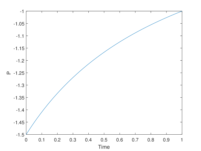
Figure 1: The curve of $P(t)$

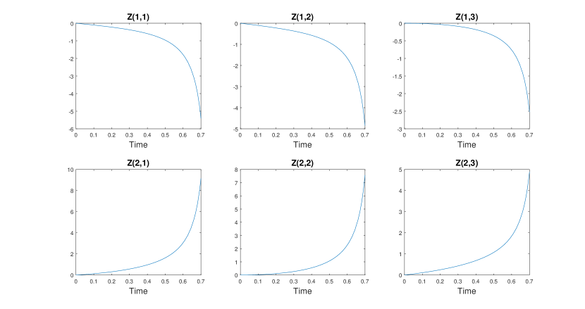
Figure 2: The curves of all entries of $Z\in\mathbb{R}^{2\times 3}$ when $t\in[0,0.7]$

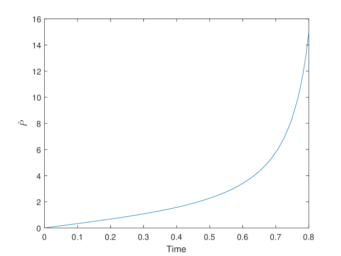
Figure 3: The curve of $\tilde{P}(t)$

V Concluding Remarks

This paper considered a class of mean field LQG social optimum problem with global drift uncertainty. Based on the soft control approach, a set of decentralized strategies is designed by optimizing the worst-case cost subject to consistent requirements in mean field approximations. Such set of strategies is further shown to be robust social optimal by perturbation analysis.

For further work, it is of interest to consider mean field team optimization with volatility-uncertain common noise. Due to common noise and volatility uncertainty, all states of agents are coupled via some high-dimensional FBSDE systems. Another interesting topic is the mean field Stackelberg game with a leader and many followers [34, 37]. The team problem with hierarchical structure is worthwhile to study further.

Appendix A Proof of Theorem II.4

Proof. Note that we only need to optimize the social cost under worst-case disturbance $J_{\rm soc}^{\rm wo}({u})$. By Theorem II.2, we can restrict to consider Problem (P2) instead of (PF). From Lemma II.4, one obtains that for (P2),

$$\mathbb{E}\int_{0}^{T}(\|\hat{x}_{i}\|^{2}+\|\hat{u}_{i}\|^{2})dt<C.$$ (A.1)

It suffices to consider all $u_{i}\in{\mathcal{U}}_{c}^{\rm F}$ such that $J_{\rm soc}^{\rm wo}({u})\leq J_{\rm soc}^{\rm wo}(\hat{u})\leq NC_{0}.$ By Lemma II.3,

$$\mathbb{E}\int_{0}^{T}\|{u}_{i}\|^{2}dt<C,\ i=1,\cdots,N,$$ (A.2)

which implies

$$\mathbb{E}\int_{0}^{T}\|{u}^{(N)}\|^{2}dt<C.$$ (A.3)

By (26) and [38, Chaper 7], we have

$$\mathbb{E}\int_{0}^{T}\|s\|^{2}dt\leq C_{1}\mathbb{E}\int_{0}^{T}\|u^{(N)}\|^{2}dt<C.$$

From (24),

$$dx^{(N)}\!=\!\big{[}(A\!+\!\bar{G})x^{(N)}\!+\!Bu^{(N)}\!-\!R_{2}^{-1}s\big{]}dt\!+\!\frac{1}{N}\!\sum_{i=1}^{N}\sigma dW_{i},$$

which together with (A.3) implies $\mathbb{E}\int_{0}^{T}\|{x}^{(N)}\|^{2}dt\!<C\!\!.$ This with (A.2) leads to

$$\mathbb{E}\int_{0}^{T}(\|{x}_{i}\|^{2}+\|{u}_{i}\|^{2}+\|s\|^{2})dt<C.$$ (A.4)

Let $\tilde{x}_{i}=x_{i}-\hat{x}_{i}$, $\tilde{u}_{i}=u_{i}-\hat{u}_{i}$, $i=1,\cdots,N$, $\tilde{x}^{(N)}=\frac{1}{N}\sum_{j=1}^{N}\tilde{x}_{j}$ and $\tilde{s}=s-\hat{s}$. Then by (24),

$$d\tilde{x}_{i}= (A\tilde{x}_{i}+\bar{G}\tilde{x}^{(N)}+B\tilde{u}_{i}-R_{2}^{-1}\tilde{s})dt,\ \tilde{x}_{i}(0)=0.$$ (A.5)

$$d\tilde{s}= -\big{[}(A+\bar{G})^{T}\tilde{s}+PB\tilde{u}^{(N)}\big{]}dt$$ (A.6)

$$+\frac{1}{N}\sum_{i=1}^{N}\sum_{j=1}^{N}\tilde{\beta}_{i}^{j}dW_{j},\ \tilde{s}(T)=0.$$ (A.7)

By (A.1) and (A.4),

$$\mathbb{E}\int_{0}^{T}(\|\tilde{x}_{i}\|^{2}+\|\tilde{u}_{i}\|^{2}+\|\tilde{s}\|^{2})dt<C.$$ (A.8)

From (26), we have

$$J^{\rm F}_{\rm soc}(u)= \frac{1}{2}\sum_{i=1}^{N}\mathbb{E}\int_{0}^{T}\Big{[}\big{\|}\hat{x}_{i}-\Gamma\hat{x}^{(N)}-\eta+\tilde{x}_{i}$$ (A.9)

$$-\Gamma\tilde{x}^{(N)}\big{\|}^{2}_{Q}+\big{\|}\hat{u}_{i}+\tilde{u}_{i}\big{\|}^{2}_{R_{1}}$$

$$-\big{\|}P(\hat{x}^{(N)}+\tilde{x}^{(N)})+\hat{s}+\tilde{s}\big{\|}^{2}_{R_{2}^{-1}}\Big{]}dt$$

$$+\frac{1}{2}\mathbb{E}\big{\|}\hat{x}_{i}(T)+\tilde{x}_{i}(T)\big{\|}^{2}_{H}$$

$$= \sum_{i=1}^{N}(J_{i}^{\rm F}(\hat{u})+\tilde{J}_{i}^{\rm F}(\tilde{u})+I_{i}),$$

where

$$\tilde{J}_{i}^{\rm F}(\tilde{u})\stackrel{{\scriptstyle\Delta}}{{=}} \frac{1}{2}\mathbb{E}\int_{0}^{T}\big{[}\|\tilde{x}_{i}-\Gamma\tilde{x}^{(N)}\|^{2}_{Q}+\|\tilde{u}_{i}\|^{2}_{R_{1}}$$

$$-\|P\tilde{x}^{(N)}\|^{2}_{R_{2}}\big{]}dt+\frac{1}{2}\mathbb{E}\big{\|}\tilde{x}_{i}(T)\big{\|}^{2}_{H},$$

$$I_{i}= \mathbb{E}\int_{0}^{T}\Big{[}\big{(}\hat{x}_{i}-\Gamma\hat{x}^{(N)}-\eta\big{)}^{T}Q\big{(}\tilde{x}_{i}-\Gamma\tilde{x}^{(N)}\big{)}$$

$$+\hat{u}_{i}^{T}R_{1}\tilde{u}_{i}-\big{(}P(\hat{x}^{(N)}+\hat{s})\big{)}^{T}{R_{2}^{-1}}(P\tilde{x}^{(N)}$$

$$+\tilde{s})\Big{]}dt+\mathbb{E}[\hat{x}_{i}^{T}(T)H\tilde{x}_{i}(T)].$$

By Lemma II.1, Problem (P2) is uniformly convex for $N\geq N_{0}$, which with Proposition II.1 gives $\tilde{J}_{i}(\tilde{u})\geq 0$. We now prove $\frac{1}{N}\sum_{i=1}^{N}I_{i}=O(\frac{1}{\sqrt{N}})$. By straightforward computation,

$$\sum_{i=1}^{N}I_{i}=\sum_{i=1}^{N}\mathbb{E}\int_{0}^{T}\Big{\{}\tilde{x}_{i}^{T}\big{[}Q(\hat{x}_{i}-\Gamma\hat{x}^{(N)}-\eta)$$ (A.10)

$$-\Gamma^{T}Q((I-\Gamma)\hat{x}^{(N)}-\eta)\big{]}+\hat{u}_{i}^{T}R_{1}\tilde{u}_{i}\Big{\}}dt$$ (A.11)

$$-N\mathbb{E}\int_{0}^{T}\big{(}P\hat{x}^{(N)}+\hat{s}\big{)}^{T}{R_{2}^{-1}}(P\tilde{x}^{(N)}+\tilde{s})dt$$ (A.12)

$$+\sum_{i=1}^{N}\mathbb{E}[\hat{x}_{i}^{T}(T)H\tilde{x}_{i}(T)]$$ (A.13)

$$= \sum_{i=1}^{N}\mathbb{E}\int_{0}^{T}\Big{\{}\tilde{x}_{i}^{T}(Q\hat{x}_{i}-\Psi\bar{x}-\eta)+\hat{u}_{i}^{T}R_{1}\tilde{u}_{i}$$ (A.14)

$$-\big{(}P\bar{x}+\hat{s}\big{)}^{T}{R_{2}^{-1}}P\tilde{x}_{i}\Big{\}}dt$$ (A.15)

$$+\sum_{i=1}^{N}\mathbb{E}\!\int_{0}^{T}\!\!\xi^{T}\big{[}(\Psi\!-\!PR_{2}^{-1}P)\tilde{x}_{i}\!-\!PR_{2}^{-1}\tilde{s}\big{]}dt$$ (A.16)

$$-N\mathbb{E}\!\!\int_{0}^{T}\!\!(P\bar{x}+\hat{s})^{T}R_{2}^{-1}\tilde{s}dt+\sum_{i=1}^{N}\mathbb{E}\|\hat{x}_{i}^{T}(T)\|_{H}^{2},$$ (A.17)

where $\xi=\hat{x}^{(N)}-\bar{x}$. By (82) and (88),

$$d\hat{k}_{i}= \big{\{}-A^{T}\hat{k}_{i}-Q\hat{x}_{i}+(\Psi\bar{x}+\bar{\eta})+PR_{2}^{-1}(P\bar{x}+\bar{s})$$ (A.18)

$$-\!\bar{G}^{T}v\!+\!KG(\hat{x}^{(N)}-\bar{x})-KR_{2}^{-1}(\hat{s}-\bar{s})\big{\}}dt$$ (A.19)

$$+K\sigma dW_{i},\ \hat{k}_{i}(T)=H\hat{x}_{i}(T).$$ (A.20)

By (A.5) and Itô’s formula,

$$\sum_{i=1}^{N}\mathbb{E}[\hat{x}_{i}^{T}(T)H\tilde{x}_{i}(T)]$$

$$= \sum_{i=1}^{N}\mathbb{E}\int_{0}^{T}\Big{\{}-\big{[}Q\hat{x}_{i}-(\Psi\bar{x}+\bar{\eta})-PR_{2}^{-1}(P\bar{x}+\bar{s})$$

$$+\bar{G}^{T}v-KG(\hat{x}^{(N)}-\bar{x})+KR_{2}^{-1}(\hat{s}-\bar{s})\big{]}^{T}\tilde{x}_{i}$$

$$+\hat{k}_{i}^{T}(\bar{G}\tilde{x}^{(N)}+B\tilde{u}_{i}-R_{2}^{-1}\tilde{s})\Big{\}}dt,$$

and

$$0= \sum_{i=1}^{N}\mathbb{E}[l^{T}(T)\tilde{s}(T)-l^{T}(0)\tilde{s}(0)]$$

$$= N\mathbb{E}\int_{0}^{T}[R_{2}^{-1}v+R_{2}^{-1}(P\bar{x}+\bar{s})]^{T}\tilde{s}dt$$

$$-N\mathbb{E}\int_{0}^{T}(l^{T}PB\tilde{u}^{(N)})dt.$$

The above two equations lead to

$$\sum_{i=1}^{N}\mathbb{E}[\hat{x}_{i}^{T}(T)H\tilde{x}_{i}(T)]$$

$$= \sum_{i=1}^{N}\mathbb{E}\int_{0}^{T}\Big{\{}-\big{[}Q\hat{x}_{i}-(\Psi\bar{x}+\bar{\eta})-PR_{2}^{-1}(P\bar{x}+\bar{s})$$

$$-KG(\hat{x}^{(N)}-\bar{x})+KR_{2}^{-1}(\hat{s}-\bar{s})\big{]}^{T}\tilde{x}_{i}$$

$$-\hat{u}_{i}^{T}R_{1}\tilde{u}_{i}+(\hat{k}^{(N)}-v)^{T}\bar{G}\tilde{x}_{i}$$

$$-(\hat{k}^{(N)}-v)R_{2}^{-1}\tilde{s}+(P\bar{x}+\bar{s})^{T}R_{2}^{-1}\tilde{s}\Big{\}}dt.$$

From this and (A.10),

$$\sum_{i=1}^{N}I_{i}= \sum_{i=1}^{N}\mathbb{E}\int_{0}^{T}\big{[}\xi^{T}(\Psi-PR_{2}^{-1}P+KG)\tilde{x}_{i}$$

$$+(\hat{k}^{(N)}-v)^{T}(\bar{G}\tilde{x}_{i}-R_{2}^{-1}\tilde{s})$$

$$+((P+K)\tilde{x}_{i}+\tilde{s})R_{2}^{-1}(\bar{s}-\hat{s})\big{]}dt.$$

By Lemmas II.2, II.5 and Schwarz inequality, we obtain

$$\frac{1}{N}\sum_{i=1}^{N}I_{i}=O(\frac{1}{\sqrt{N}}).$$

From this with (A.9), the theorem follows. $\hfill{\Box}$

Appendix B Proof of Theorem III.2

To prove Theorem III.2, we need three lemmas.

Lemma B.1

Assume that (A0)-(A1), (A5)-(A8) hold. For Problem (PI), we have

$$\mathbb{E}\int_{0}^{\infty}e^{-\rho t}\big{(}\|\hat{x}^{(N)}-\bar{x}\|^{2}+\|\hat{s}-\bar{s}\|^{2}\big{)}dt=O(\frac{1}{N}).$$ (B.1)

Proof. By a similar argument to (93)-(95), we obtain

$$d\xi= (\bar{A}+\bar{G})\xi dt-{R_{2}^{-1}}\chi dt+\frac{1}{N}\sum_{i=1}^{N}\sigma dW_{i},$$

$$\textstyle{\xi(0)=\frac{1}{N}\sum_{i=1}^{N}x_{i0}-\bar{x}_{0}},$$

$$d\chi= -\big{[}(A+\bar{G})^{T}\chi+PBR_{1}^{-1}B^{T}K\xi\big{]}dt$$

$$+\frac{1}{N}\sum_{i=1}^{N}\sum_{j=1}^{N}(\beta_{i}^{j}-\frac{\sigma}{N})dW_{j},$$

where $\xi{=}\hat{x}^{(N)}-\bar{x}$ and $\chi{=}\hat{s}-\bar{s}$. By Itô’s formula and (A8), we have $\chi=\tilde{P}\xi+\psi$, where $\tilde{P}$ is given by (133). Denote $\Upsilon=\bar{A}+\bar{G}-R_{2}^{-1}\tilde{P}$. Then

$$\xi(t)= e^{\Upsilon t}\xi(0)+\frac{1}{N}\int_{0}^{t}e^{\Upsilon(t-\mu)}\sum_{i=1}^{N}\sigma dW_{i}(\mu).$$

This with (A8) gives $\mathbb{E}\int_{0}^{\infty}e^{-\rho t}\|\xi(t)\|^{2}dt=O({1}/{N})$. $\Box$

Lemma B.2

Assume that (A0)-(A1), (A5)-(A8) hold. For Problem (PI) and any $N$,

$$\max_{1\leq i\leq N}\mathbb{E}\int_{0}^{\infty}e^{-\rho t}\left(\|\hat{x}_{i}\|^{2}+\|\hat{u}_{i}\|^{2}\right)dt<\infty.$$ (B.2)

Proof. By (A7) and Lemma B.1, we obtain that

$$\mathbb{E}\int_{0}^{\infty}e^{-\rho t}(\|\hat{x}^{(N)}(t)\|^{2}+\|\hat{s}(t)\|^{2})dt<\infty.$$

Note that $\bar{A}-\frac{\rho}{2}I$ is Hurwitz. By Schwarz’s inequality,

$$\mathbb{E}\int_{0}^{\infty}e^{-\rho t}\|\hat{x}_{i}(t)\|^{2}dt$$

$$\leq\ C\!+\!3\mathbb{E}\!\int_{0}^{\infty}\!\!e^{-\rho\mu}\|g(\mu)\|^{2}\!\int_{\mu}^{\infty}\!\!t\big{\|}e^{(\bar{A}-\frac{\rho}{2}I)(t-\mu)}\big{\|}^{2}dtd\mu$$

$$+3C\mathbb{E}\!\int_{0}^{\infty}\!\!e^{-\rho\mu}\|\sigma(\mu)\|^{2}\!\int_{\mu}^{\infty}\!\!\big{\|}e^{(\bar{A}-\frac{\rho}{2}I)(t-\mu)}\sigma\big{\|}^{2}dtd\mu$$

$$\leq\ C+3C\mathbb{E}\int_{0}^{\infty}e^{-\rho\mu}\|g(\mu)\|^{2}d\mu$$

$$+3C\mathbb{E}\int_{0}^{\infty}e^{-\rho\mu}\|\sigma(\mu)\|^{2}d\mu\leq C_{1}.$$

This with (A7) completes the proof. $\Box$

Lemma B.3

Assume $A-\frac{\rho}{2}I$ is Hurwitz. Then

$$\mathbb{E}\int_{0}^{\infty}e^{-\rho t}\|\hat{k}^{(N)}-v\|^{2}dt\leq O(1/N).$$

Proof. By (127) and some elementary computations, we obtain $d\vartheta(t)=-(A-\frac{\rho}{2}I)^{T}\vartheta(t)dt,$ where $\vartheta=v-K\bar{x}-\varphi$. This leads to $\vartheta(t)=e^{-(A-\frac{\rho}{2}I)t}\vartheta(0)$. Since $A-\frac{\rho}{2}I$ is Hurwitz, and $\vartheta\in C_{\rho/2}([0,\infty),\mathbb{R}^{n})$, then we have $\vartheta(t)\equiv 0$, which implies $v=K\bar{x}+\varphi$. By Lemma B.1, $\int_{0}^{\infty}e^{-\rho t}\mathbb{E}\|\hat{k}^{(N)}-v\|^{2}dt\leq O(1/N).$ This completes the proof. $\Box$

Proof of Theorem III.2. As in the proof of Theorem II.4, we restrict to Problem (P2^′). It suffices to consider all $u_{i}\in{\mathcal{U}}_{c}$ such that $\sup_{f\in{\mathcal{U}}_{c}}J_{\rm soc}({u},f)\leq\sup_{f\in{\mathcal{U}}_{c}}J_{\rm soc}(\hat{u},f)\leq NC_{0}.$ Taking $f=0$, we have

$$\mathbb{E}\int_{0}^{\infty}e^{-\rho t}\|{u}_{i}\|^{2}dt<C.$$ (B.3)

By (110) and [29], we have

$$\mathbb{E}\int_{0}^{\infty}e^{-\rho t}\|s\|^{2}dt\leq C_{1}\mathbb{E}\int_{0}^{\infty}e^{-\rho t}\|u^{(N)}\|^{2}dt<C.$$

Noticing $A+\bar{G}-\frac{\rho}{2}I$ is Hurwitz, one can obtain $\mathbb{E}\int_{0}^{\infty}e^{-\rho t}\|{x}^{(N)}\|^{2}dt<C$ which with (B.3) implies

$$\mathbb{E}\int_{0}^{\infty}e^{-\rho t}\big{(}\|{x}_{i}\|^{2}+\|{u}_{i}\|^{2}+\|s\|^{2}\big{)}dt\leq C.$$ (B.4)

From this and (B.2),

$$\mathbb{E}\int_{0}^{\infty}(\|\tilde{x}_{i}\|^{2}+\|\tilde{u}_{i}\|^{2}+\|\tilde{s}\|^{2})dt<C.$$ (B.5)

We have $J_{\rm soc}(u)=\sum_{i=1}^{N}(J_{i}(\hat{u})+\tilde{J}_{i}(\tilde{u})+\mathcal{I}_{i}),$ where

$$\tilde{J}_{i}(\tilde{u})\stackrel{{\scriptstyle\Delta}}{{=}}\frac{1}{2}\mathbb{E} \int_{0}^{\infty}e^{-\rho t}\big{[}\|\tilde{x}_{i}-\Gamma\tilde{x}^{(N)}\|^{2}_{Q}$$

$$+\|\tilde{u}_{i}\|^{2}_{R_{1}}-\|P\tilde{x}^{(N)}\|^{2}_{R_{2}}\big{]}dt,$$

$$\mathcal{I}_{i}\stackrel{{\scriptstyle\Delta}}{{=}}\mathbb{E} \int_{0}^{\infty}e^{-\rho t}\Big{[}\big{(}\hat{x}_{i}-\Gamma\hat{x}^{(N)}-\eta\big{)}^{T}Q\big{(}\tilde{x}_{i}$$

$$-\Gamma\tilde{x}^{(N)}\big{)}+\hat{u}_{i}^{T}R_{1}\tilde{u}_{i}$$

$$-\big{(}P(\hat{x}^{(N)}+s)\big{)}^{T}{R_{2}^{-1}}(P\tilde{x}^{(N)}+\tilde{s})\Big{]}dt.$$

From Lemma III.1 and Proposition III.1, $\tilde{J}_{i}(\tilde{u})\geq 0$ for $N\geq N_{0}$. By making use of Itô’s formula and straightforward computations,

$$\sum_{i=1}^{N}\mathcal{I}_{i}= \sum_{i=1}^{N}\mathbb{E}\int_{0}^{\infty}e^{-\rho t}\Big{\{}\tilde{x}_{i}^{T}\big{[}Q\hat{x}_{i}-\Psi\bar{x}-\bar{\eta}\big{]}$$

$$+\hat{u}_{i}^{T}R_{1}\tilde{u}_{i}-\big{(}P\bar{x}+\hat{s}\big{)}^{T}{R_{2}^{-1}}P\tilde{x}_{i}\Big{\}}dt$$

$$+\sum_{i=1}^{N}\mathbb{E}\int_{0}^{\infty}e^{-\rho t}\xi^{T}[(\Psi-PR_{2}^{-1}P)\tilde{x}_{i}-PR_{2}^{-1}\tilde{s}]dt$$

$$-N\mathbb{E}\int_{0}^{\infty}e^{-\rho t}(P\bar{x}+\hat{s})^{T}R_{2}^{-1}\tilde{s}dt,$$

$$= \sum_{i=1}^{N}\mathbb{E}\int_{0}^{\infty}e^{-\rho t}\big{[}\xi^{T}(\Psi-PR_{2}^{-1}P+KG)\tilde{x}_{i}$$

$$+(\hat{k}^{(N)}-v)^{T}(\bar{G}\tilde{x}_{i}-R_{2}^{-1}\tilde{s})$$

$$+((P+K)\tilde{x}_{i}+\tilde{s})R_{2}^{-1}(\bar{s}-\hat{s})\big{]}dt.$$

From (B.1) and (B.5), we obtain

$$\frac{1}{N}\sum_{i=1}^{N}\mathcal{I}_{i}=O(\frac{1}{\sqrt{N}}).$$

$\Box$

Bingchang Wang received the M.Sc. degree in Mathematics from Central South University, Changsha, China, in 2008, and the Ph.D. degree in System Theory from Academy of Mathematics and Systems Science, Chinese Academy of Sciences, Beijing, China, in 2011. From September 2011 to August 2012, he was with Department of Electrical and Computer Engineering, University of Alberta, Canada, as a Postdoctoral Fellow. From September 2012 to September 2013, he was with School of Electrical Engineering and Computer Science, University of Newcastle, Australia, as a Research Academic. From October 2013, he has been with School of Control Science and Engineering, Shandong University, China, as an associate Professor. He held visiting appointments as a Research Associate with Carleton University, Canada, from November 2014 to May 2015, and with the Hong Kong Polytechnic University from November 2016 to January 2017. His current research interests include mean field games, stochastic control, multiagent systems and event based control. He received the IEEE CSS Beijing Chapter Young Author Prize in 2018.

Jianhui Huang Jianhui Huang received his B.S. degree in operational research and control theory, M.Sc. degree in probability theory and mathematical statistics from the School of Mathematics and System Sciences, Shandong University, Jinan, China, respectively, in 1998 and 2001. He received his Ph.D. degree in mathematical finance from the Department of Mathematical and Statistical Sciences, University of Alberta, Edmonton, Canada, in 2007. Since 2007, he has been with The Hong Kong Polytechnic University, where he is currently an assistant professor at the Department of Applied Mathematics. His current research interests include stochastic control and optimization, stochastic dynamic games, large population systems and their applications. He has published in journals such as SIAM Journal on Control and Optimization, IEEE Transactions on Automatic Control and Automatica.

Ji-Feng Zhang (M’92-SM’97-F’14) received the B.S. degree in mathematics from Shandong University, China, in 1985 and the Ph.D. degree from the Institute of Systems Science (ISS), Chinese Academy of Sciences (CAS), China, in 1991. Since 1985, he has been with the ISS, CAS, and now is the Director of ISS. He is a Deputy Editor-in-Chief of Science China Information Sciences, and was the Editor-in-Chief of Journal of Systems Science and Mathematical Sciences, the founding Editor-in-Chief of All About Systems and Control, a Managing Editor of Journal of Systems Science and Complexity, Deputy Editor-in-Chief of Acta Automatica Sinica, Control Theory and Applications and Systems Engineering — Theory and Practice, Associate Editor of several other journals, including IEEE Trans. on Automatic Control, SIAM Journal on Control and Optimization etc. His current research interests include system modeling, adaptive control, stochastic systems, and multi-agent systems. Besides IEEE Fellow, Dr. Zhang is also an IFAC Fellow, CAA Fellow, a Member of the European Academy of Sciences and Arts, and an Academician of the International Academy for Systems and Cybernetic Sciences. He received twice the Second Prize of the State Natural Science Award of China in 2010 and 2015, respectively, the Distinguished Young Scholar Fund from National Natural Science Foundation of China in 1997, the First Prize of the Young Scientist Award of CAS in 1995, the Outstanding Advisor Award of CAS in 2007, 2008 and 2009, respectively. He is a Vice-Chair of the IFAC Technical Board, and a Convenor of Systems Science Discipline, Academic Degree Committee of the State Council of China; and was a member of the Board of Governors, IEEE Control Systems Society; Vice President of the Systems Engineering Society of China, Vice President of the Chinese Association of Automation, General Co-Chair of the 33rd and the 36th Chinese Control Conferences; IPC Chair of the 2012 IEEE Conference on Control Applications, the 9th World Congress on Intelligent Control and Automation, and the 17th IFAC Symposium on System Identification; and is an IPC Vice-Chair of the 20th IFAC World Congress, etc.

References

• [1] H. Abou-Kandil, G. Freiling, V. Ionescu, and G. Jank, Matrix Riccati Equations in Control and Systems Theory, Birkhiiuser Verlag, 2003.
• [2] J. Arabneydi and A. Mahajan, “Team-optimal solution of finite number of mean-field coupled LQG subsystems”, Proc. 54th IEEE Conf. Decision Control, pp. 5308-5313, Osaka, Japan, 2015.
• [3] T. Basar and P. Bernhard, $H^{\infty}$-optimal Control and Related Minimax Design Problems: A Dynamic Game Approach, 2nd ed., Boston, MA: Birkhauser, 1995.
• [4] A. Bensoussan, J. Frehse, and P. Yam, Mean Field Games and Mean Field Type Control Theory, Springer, New York, 2013.
• [5] W. A. van den Broek, J. C. Engwerda, and J. M. Schumacher, “Robust equilibria in indefinite linear-quadratic differential games”, Journal of Optimization Theory and Applications, vol. 119, no. 3, pp. 565-595, 2003.
• [6] P. E. Caines, M. Huang, and R. P. Malhame, “Mean field games”, in Handbook of Dynamic Game Theory, T. Basar and G. Zaccour Eds., Springer, Berlin, 2017.
• [7] R. Carmona and F. Delarue, “Probabilistic analysis of mean-field games”, SIAM J. Control Optim., vol. 51, no. 4, pp. 2705-2734, 2013.
• [8] J. Engwerda, “A numerical algorithm to find soft-constrained Nash equilibria in scalar LQ-games”, International Journal of Control, vol. 79, no. 6, pp. 592-603, 2006.
• [9] G. Freiling and G. Jank, “Existence and comparison theorems for algebraic and continuous-time Riccati differential and difference equations”, Journal of Dynamical Control Systems, 2, pp. 529-547, 1996.
• [10] D. A. Gomes and J. Saude, “Mean field games models–a brief survey”, Dynamic Games and Applications, vol. 4, no. 2, pp. 110-154, 2014.
• [11] Y. C. Ho, “Team decision theory and information structures”, Proceedings of IEEE, vol. 68, pp. 644-654, 1980.
• [12] R. A. Horn and C. R. Johnson, Matrix Analysis, 2nd ed. Cambridge University Press, 2013.
• [13] J. Huang and M. Huang, “Mean field LQG games with model uncertainty”, Proc. 52nd IEEE Conf. Decision Control, pp. 3103-3108, Florence, Italy, 2013.
• [14] J. Huang and M. Huang, “Robust mean field linear-quadratic-Gaussian games with model uncertainty”, SIAM J. Control Optim., vol. 55, no. 5, pp. 2811-2840, 2017.
• [15] M. Huang, “Large-population LQG games involving a major player: the Nash certainty equivalence principle”, SIAM J. Control Optim., vol. 48, pp. 3318-3353, 2010.
• [16] M. Huang, P. E. Caines, and R. P. Malhamé, “Individual and mass behaviour in large population stochastic wireless power control problems: Centralized and Nash equilibrium solutions”, Proc. 52nd IEEE Conf. Decision Control, pp. 98-103, Maui, HI, 2003.
• [17] M. Huang, P. E. Caines, and R. P. Malhamé, “Large-population cost-coupled LQG problems with non-uniform agents: individual-mass behavior and decentralized $\varepsilon$-Nash equilibria”, IEEE Trans. Autom. Control, vol. 52, pp. 1560-1571, 2007.
• [18] M. Huang, P. Caines, and R. Malhame, “Social optima in mean field LQG control: centralized and decentralized strategies”, IEEE Trans. Autom. Control, vol. 57, no. 7, pp. 1736-1751, 2012.
• [19] M. Huang, R. P. Malhamé, and P. E. Caines, “Large population stochastic dynamic games: closed-loop McKean-Vlasov systems and the Nash certainty equivalence principle”, Communication in Information and Systems, vol. 6, pp. 221-251, 2006.
• [20] M. Huang and L. Nguyen, “Linear-quadratic mean field teams with a major agent”, Proc. 55th IEEE Conf. Decision Control, pp. 6958-6963, Las Vegas, USA, 2016.
• [21] J. M. Lasry, and P. L. Lions, “Mean field games”, Japn. J. Math., vol. 2, pp. 229-260, 2007.
• [22] T. Li and J. F. Zhang, “Asymptotically optimal decentralized control for large population stochastic multiagent systems”, IEEE Trans. Automat. Control, vol. 53, no. 7, pp. 1643-1660, August 2008.
• [23] A. Lim and X. Y. Zhou, “Stochastic optimal LQR control with integral quadratic constraints and indefinite control weights”, IEEE Trans. Autom. Control, vol. 44, no. 7, pp. 1359-1369, July, 1999.
• [24] S. Li, W. Zhang, and L. Zhao “On social optima of non-cooperative mean field games”, Proc. 55th IEEE Conf. Decision Control, pp. 3584-3590, Las Vegas, USA, 2016.
• [25] J. Ma and J. Yong, Forward-backward Stochastic Differential Equations and their Applications, Lecture Notes in Math. 1702, Springer-Verlag, New York, 1999.
• [26] B. P. Molinari, “The time-invariant linear-quadratic optimal control problem”, Automatica, vol. 13, pp. 347-357, 1977.
• [27] J. Moon and T. Basar, “Linear quadratic risk-sensitive and robust mean field games”, IEEE Trans. Autom. Control, vol. 62, no. 3, 2017.
• [28] J. Sun, X. Li, and J. Yong, “Open-loop and closed-loop solvabilities for stochastic linear quadratic optimal control problems”, SIAM J. Control Optim., vol. 54, no. 5, 2274-2308, 2016.
• [29] J. Sun, and J. Yong. Stochastic linear quadratic optimal control problems in infinite horizon, Applied Mathematics & Optimization, pp. 1C39, 2017.
• [30] H. Tembine, D. Bauso, and T. Basar, “Robust linear quadratic mean-field games in crowd-seeking social networks”, Proc. 52nd IEEE Conf. Decision Control, pp. 3134-3139, Florence, Italy, 2013.
• [31] B. C. Wang and J. Huang, “Social optima in robust mean field LQG control”, Proc. 11th Asian Control Conference, pp. 2089-2094, Gold Coast, Australia, 2017.
• [32] B. C. Wang and J. F. Zhang, “Mean field games for large-population multiagent systems with Markov jump parameters”, SIAM J. Control Optim., vol. 50, no. 4, pp. 2308-2334, 2012.
• [33] B. C. Wang and J. F. Zhang, “Distributed control of multi-agent systems with random parameters and a major agent”, Automatica, vol. 48, no. 9, 2093-2106, 2012.
• [34] B. C. Wang and J. F. Zhang, “Hierarchical mean field games for multiagent systems with tracking-type costs: Distributed $\varepsilon$-Stackelberg equilibria”, IEEE Trans. Autom. Control, vol. 59, no. 8, 2241-2247, 2014.
• [35] B. C. Wang and J. F. Zhang, “Social optima in mean field linear-quadratic-Gaussian models with Markov jump parameters”, SIAM J. Control Optim., vol. 55, no. 1, pp. 429-456, 2017.
• [36] G. Weintraub, C. Benkard, and B. van Roy, “Markov perfect industry dynamics with many firms”, Econometrica, vol. 76, no. 6, pp. 1375-1411, 2008.
• [37] J. Xu, J. Shi, and H. Zhang, A leader-follower stochastic linear quadratic differential game with time delay. Science China Information Sciences, vol. 61, no. 3-13, 2018.
• [38] J. Yong and X. Y. Zhou, Stochastic Controls: Hamiltonian Systems and HJB Equations, Springer-Verlag, New York, 1999.
• [39] H. Zhang and Q. Qi, Optimal control for mean-field system: Discrete-time case. Proc. 55th IEEE Conf. Decision Control, pp. 4474-4480, Las Vegas, USA, 2016.
• [40] S. Zhang, J. Xiong, and X. Liu, Stochastic maximum principle for partially observed forward-backward stochastic differential equations with jumps and regime switching, Science China Information Sciences, vol. 61, no. 7, pp. 1-13, 2018.