The Use of Binary Choice Forests to Model and Estimate Discrete Choices

Abstract

We show the equivalence of discrete choice models and a forest of binary decision trees. This suggests that standard machine learning techniques based on random forests can serve to estimate discrete choice models with an interpretable output: the underlying trees can be viewed as the internal choice process of customers. Our data-driven theoretical results show that random forests can predict the choice probability of any discrete choice model consistently. Moreover, our algorithm predicts unseen assortments with mechanisms and errors that can be theoretically analyzed. We also prove that the splitting criterion in random forests, the Gini index, is capable of recovering preference rankings of customers. The framework has unique practical advantages: it can capture behavioral patterns such as irrationality or sequential searches; it handles nonstandard formats of training data that result from aggregation; it can measure product importance based on how frequently a random customer would make decisions depending on the presence of the product; it can also incorporate price information and customer features. Our numerical results show that using random forests to estimate customer choices can outperform the best parametric models in synthetic and real datasets when presented with enough data or when the underlying discrete choice model cannot be correctly specified by existing parametric models.

1 Introduction

Discrete choice models (DCM) have become central to revenue management and e-commerce as they enable firms to predict consumer’s choice behavior when confronted with a given assortment of products. Firms that can get inside the mind of their consumers enjoy unique advantages that allow them to implement effective strategies to improve profits or market shares. Firms can then further invest in technologies that sharpen their predictive power. This virtuous cycle has created a number of market juggernauts while those incapable of playing in this field are disappearing from the landscape.

To understand and predict consumers’ choice behavior, academics and practitioners have proposed several frameworks, some of which are widely adopted in the industry. One ubiquitous framework is model-then-estimate. In this framework, a parametric DCM is proposed to explain how a consumer chooses a product when offered an assortment. The parameters are then estimated using historical data. Once the model has been estimated properly, it can then be used as a workhorse to predict the choice behavior of future consumers.

In the model-then-estimate framework, there is a trade-off between flexibility and accuracy. A flexible DCM incorporates a wide range of patterns of consumers’ behavior, but it may be difficult to estimate and may overfit the training data. A parsimonious model, on the other hand, may fail to capture complex choice patterns in the data. Even estimated correctly, it would be misspecified and not perform well in prediction. The key to a successful model is to reach a delicate balance between flexibility and predictability. Not surprisingly, it is not straightforward to find the “sweet spot” when selecting among the large class of parametric DCMs. For this reason a variety of models are usually tested and calibrated and the one which performs the best on test data is then used until more data is collected and the process is repeated.

Another framework favored by data scientists is to estimate without models. Advanced machine learning algorithms are applied to historical sales data, and used to predict future choice behavior. The framework skips “modeling” entirely and does not attempt to understand the rationality (or irrationality) hidden behind the patterns observed in the training data. With engineering tweaks, the algorithms can be implemented efficiently and capture a wide range of choice behavior. For example, neural networks are known to be able to approximate any continuous functions.

This approach may sound appealing: if an algorithm achieves impressive accuracy when predicting the choice behavior of consumers, why do we care about the actual rationale in consumers’ minds when they make choices? There are two counterarguments. First, the firm may be interested in not only making accurate predictions but also in other goals such as finding an optimal assortment that maximizes the expected revenue, which may not have appeared in the data. Without a proper model, it is unclear if the goal can be formulated as an optimization problem. Second, when the market environment is subject to secular changes, having a reasonable model often provides a certain degree of generalizability while black-box algorithms may fail to capture an obvious pattern just because the pattern has not appeared frequently in the past.

In this paper, we introduce a data-driven framework which we call estimate-and-model that combines machine learning with interpretable models, and thus retains the strengths of both frameworks mentioned previously. The model we propose, binary choice forests, is a mixture of binary choice trees, each of which reflects the internal decision-making process of a potential customer. We show that the binary choice forest can be used to approximate any DCM, and is thus sufficiently flexible. Moreover, it can be efficiently estimated using random forests (Breiman, 2001), a popular machine learning technique that has stood the test of time. Random forests are easy to implement using R or Python (Pedregosa et al., 2011; Liaw and Wiener, 2002) and have been shown to have extraordinary predictive power in other applications. We provide theoretical analyses: as the sample size increases, random forests can successfully recover the binary choice forest, and thus any DCM; random forests serve as adaptive nearest neighbors and effectively use the historical data to extrapolate the choice of future customers; moreover, the splitting criterion used by the random forests is intrinsically connected to the preference ranking of customers.

Besides the theoretical properties, the framework we propose has the following practical advantages: (1) It can capture patterns of behavior that elude other models, such as irregularity and sequential searches (Weitzman, 1979); details can be found in Section 5.1. (2) It can deal with nonstandard formats of historical data, which is a major challenge in practice; details can be found in Section 5.2. (3) It can return an importance index for all products, based on how frequently a random customer would make decisions depending on the presence of the product; details can be found in Section 5.3. (4) It can incorporate prices and reflect the information in the decision-making of consumers. (5) It can naturally incorporate customer features and is compatible with personalized online retailing.

1.1 Literature Review

We first review DCMs proposed in the literature following the model-then-estimate framework, in the order of increasing flexibility but more difficult estimation. The independent demand model and the MNL model (McFadden, 1973) have very few parameters (one per product), which are easy to estimate (Train, 2009). Although the MNL model is still widely used, its inherent property of independence of irrelevant alternatives (IIA) has been criticized for being unrealistic (see Anderson et al. 1992 for more details). The nested logit model, the Markov chain DCM, the mixed logit model and the rank-based DCM (see, e.g., Williams 1977; Train 2009; Farias et al. 2013; Blanchet et al. 2016) are able to capture more complex choice behavior than the MNL model. In fact, the mixed logit model and the rank-based DCM can approximate any random utility model (RUM), encompassing an important class of DCMs. The estimation of these models is challenging, but there has been exciting progress in recent years (Farias et al., 2013; van Ryzin and Vulcano, 2014, 2017; Şimşek and Topaloglu, 2018; Jagabathula et al., 2019). However, the computational feasibility and susceptibility to overfitting remain a challenge in practice. In addition, the class of RUM belongs to the class of regular models with the property that the probability of choosing an alternative cannot increase if the offered set is enlarged. Experimental studies show strong evidence that regularity may be violated in practice (Simonson and Tversky, 1992). Several models are proposed to capture more general behavior than RUM (Natarajan et al., 2009; Flores et al., 2017; Berbeglia, 2019; Feng et al., 2017), but it is not yet clear if the estimation for such models can be done efficiently.

The binary choice forest in this paper can be seen as a mixture of customer segments, where each segment has the choice behavior represented by a decision tree. In this sense, it is related to recent studies on consumer segmentation such as Bernstein et al. (2018); Jagabathula et al. (2018); Aouad et al. (2019). This paper focuses on the estimation of DCMs and the segments emerge as a byproduct to improve the predictive accuracy: the trees have equal weights and we do not control for the number of trees (segments). In contrast, Bernstein et al. (2018); Jagabathula et al. (2018); Aouad et al. (2019) design specific clustering/segmentation algorithms so the objectives differ. It is worth noticing that Aouad et al. (2019) also use the tree structure for market segmentation; however, their input consists of customer features while ours is the inclusion of a product.

The specifications of random forests used in this paper are introduced by Breiman (2001), although many of the ideas were discovered earlier. The readers may refer to Hastie et al. (2009) for a general introduction. Although random forests have been very successful in practice, little is known about their theoretical properties relatively. Most studies are focused on isolated setups or simplified versions of the procedure. For example, Lin and Jeon (2006) study the connection between random forests and adaptive nearest-neighbor methods under stylized assumptions. Biau and Scornet (2016) provide an excellent survey of the recent theoretical and methodological developments in the field. There are recent papers on theoretical properties (consistency and asymptotic normality) under less restrictive assumptions. Scornet et al. (2015) establish the consistency of random forests in regression problems. Wager (2014); Wager and Athey (2018) show that asymptotic normality can be established from the “honest” assumption. These three papers require the regression function to be continuous and the samples to have positive density in the input domain, which do no hold in the context of discrete choice models. We show that consistency can be established under general assumptions, using standard techniques such as concentration inequalities. Our result is similar to the consistency of single decision trees in Györfi et al. (2006); Devroye et al. (2013), but we need to handle the additional issue of resampling in random forests. Moreover, in Section 4.2 we utilize the nearest-neighbor interpretation of random forests to explain why the algorithm performs well on assortments that have not appeared in the data. Such connection is also specific to the application to discrete choice models.

A recent paper by Chen and Mišić (2019) proposes a similar tree-based DCM. They are the first to show that the so-called “decision forest” can approximate any DCMs with arbitrary precision; a similar result is proved with a different approach in this paper. Our studies differ substantially in the estimation step: we focus on random forests, while Chen and Mišić (2019) follow an optimization approach based on column generation. On the theoretical side, Chen and Mišić (2019) focus on the complexity of the optimization problem. We establish the consistency of random forests, explain why the algorithm works well for unseen assortments, and show that the estimation can accommodate the price information and aggregated choice data. For the numerical studies, Chen and Mišić (2019) focus on the irrational behavior in the data. In contrast, we investigate the performance of random forests more broadly. We find that random forests are quite robust and have good performance even compared with the Markov chain model estimated using the expectation-maximization (EM) algorithm, which has been shown to have outstanding empirical performance compared to MNL, the nested logit, the mixed logit and rank-based DCM (Berbeglia et al., 2018), especially when the training data is large. It is worth noticing that the applicability of the modeling framework in Chen and Mišić (2019) and our paper is greatly extended by an exciting recent study (Mišić, 2020) that provides an optimization framework to solve the optimal assortment planning problem for tree-based DCMs.

2 Discrete Choice Models and Binary Choice Forests

Consider a set $[N]\triangleq\left\{1,\ldots,N\right\}$ of $N$ products and define $[N]_{+}\triangleq[N]\cup\{0\}$ where $0$ represents the no-purchase option. Let $\bm{x}\in\left\{0,1\right\}^{N}$ be a binary vector representing an assortment of products, where $\bm{x}(i)=1$ indicates the inclusion of product $i$ in the assortment and $\bm{x}(i)=0$ otherwise. A discrete choice model (DCM) is a non-negative mapping $p(i,\bm{x}):[N]_{+}\times\left\{0,1\right\}^{N}\to[0,1]$ such that

$$\sum_{i\in[N]_{+}}p(i,\bm{x})=1,\quad p(i,\bm{x})=0\;\leavevmode\nobreak\ \leavevmode\nobreak\ \text{if }\leavevmode\nobreak\ \leavevmode\nobreak\ \bm{x}(i)=0.$$ (1)

Here $p(i,\bm{x})\in[0,1]$ represents the probability that a customer selects product $i$ from assortment $\bm{x}$. We refer to a subset $S$ of $[N]$ as an assortment associated with $\bm{x}\in\{0,1\}^{N}$, i.e., $i\in S$ if and only if $\bm{x}(i)=1$. In the remaining paper, we use $p(i,S)$ and $p(i,\bm{x})$ interchangeably.

A binary choice tree $t(\bm{x})$ maps $\bm{x}\in\{0,1\}^{N}$ into $[N]_{+}$ by sequentially splitting $[0,1]^{N}$ along $N$ products, as illustrated by the right panel of Figure 1. Moreover, to be consistent with DCMs, we require that $t(\bm{x})=i$ only if $\bm{x}(i)=1$. Equivalently, a binary choice tree partitions $\{0,1\}^{N}$ into a number of regions, denoted as $\{R_{i}\}$. Each $R_{i}$ corresponding to a leaf node of the tree. The tree assigns a label $c_{i}$ for all $\bm{x}\in R_{i}$. Therefore, one can write $t(\bm{x})=\sum_{R_{i}}c_{i}\cdot\mathbb{I}_{\left\{\bm{x}\in R_{i}\right\}}$. A binary choice tree representation of a partition when $N=2$ is demonstrated in Figure 1.

for tree=l sep+=.8cm,s sep+=.5cm,shape=rectangle, rounded corners, draw, align=center, top color=white, bottom color=gray!20 [$\bm{x}(1)\geq 0.5$ [1,edge label=node[midway,left]Y ] [$\bm{x}(2)\geq 0.5$,edge label=node[midway,right]N [2, edge label=node[midway,left]Y] [0, edge label=node[midway,right]N] ] ]

Figure 1: A binary choice tree representation of the partition.

A binary choice forest (BCF) is a convex combination or a mixture of multiple binary choice trees. More precisely, a binary choice forest can be written as

$$f(i,\bm{x})=\sum_{b=1}^{B}w_{b}\mathbb{I}_{\left\{t_{b}(\bm{x})=i\right\}}$$

where the $t_{b}(\bm{x})$ and $w_{b}$ are, respectively, binary choice trees and non-negative weights summing up to one. A BCF can be interpreted as decisions made by $B$ consumer types or segments, with consumers of type $b$ having weight $w_{b}$ and making decisions based on binary choice tree $t_{b}(\bm{x})$.

Notice that $f(i,\bm{x})$ maps $[N]_{+}\times\left\{0,1\right\}^{N}\mapsto[0,1]$ just like DCMs do, so a BCF is always a DCM according to the definition (1). The converse is also true by the next theorem.

Theorem 1.

Every BCF is a DCM. Every DCM can be represented as a BCF with at most $N\cdot 2^{N-1}+1$ binary choice trees.

A recent paper by Chen and Mišić (2019) has independently shown, by construction, that any choice model can be represented by a decision forest where each of the trees has depth $N+1$. Our result provides a smaller number of binary choice trees needed for the representation.

3 Data and Estimation

The main goal of this paper is to provide a practical method to estimate BCFs using random forests, which have been shown to be able to approximate all DCMs. The numerical recipe for random forests is widely available and implementable.

We assume that arriving consumers make selections independently based on an unknown DCM $p(i,\bm{x})$, and that a firm collects data of the form $(i_{t},\bm{x}_{t})$ (or equivalently $(i_{t},S_{t})$) where $\bm{x}_{t}$ is the assortment offered to the $t$th consumer and $i_{t}\in S_{t}\cup\{0\}$ is the choice made by consumer $t=1,\ldots,T$. Our goal is to use the data to construct a family of binary choice trees as a means to estimate the underlying DCM $p(i,\bm{x})$ represented by a BCF. We view the problem as a classification problem: given the input $\bm{x}$, we would like to provide a classifier that maps the input to a class label $i\in[N]_{+}$, or the class probabilities.

To this end we use a random forest as a classifier. The output of a random forest consists of $B$ individual binary decision trees (CART), $\left\{t_{b}(\bm{x})\right\}_{b=1}^{B}$, where $B$ is a tunable parameter. Although a single tree only outputs a class label in each region, the aggregation of the trees, i.e., the forest, is naturally equipped with the class probabilities. Then the choice probability of item $i$ in the assortment $\bm{x}$ is estimated as

$$\sum_{b=1}^{B}\frac{1}{B}\mathbb{I}_{\left\{t_{b}(\bm{x})=i\right\}},$$ (2)

which is a BCF measuring the proportion of trees that assign label $i\in[N]_{+}$ to input $\bm{x}$.

We now review the basic mechanism of CART and describe how it can be used to estimate random forests. The CART mechanism performs recursive binary splitting of the input space $[0,1]^{N}$, which is extended from $\left\{0,1\right\}^{N}$. In each iteration, it selects a product $i\in[N]$ and a split point to split the input space. More precisely, the split $(i,s_{i})$ divides the observations to $\left\{(i_{t},\bm{x}_{t}):\bm{x}_{t}(i)\leq s_{i}\right\}$ and $\left\{(i_{t},\bm{x}_{t}):\bm{x}_{t}(i)>s_{i}\right\}$. In our problem, because $\bm{x}_{t}\in\left\{0,1\right\}^{N}$ is at the corner of the hypercube, all split points between 0 and 1 create the same partition of the observations and thus we simply set $s_{i}\equiv 0.5$. To select a product for splitting, an empirical criterion is optimized to favor splits that create “purer” regions. That is, the resulting region should contain data points that mostly belong to the same class. We use a common measure called Gini index: $\sum_{R_{j}}\frac{t_{j}}{T}\sum_{k=0}^{N}\hat{p}_{jk}(1-\hat{p}_{jk})$ where $t_{j}$ is the number of observations in region $R_{j}$ of the partition and $\hat{p}_{jk}$ is the empirical frequency of class $k$ in $R_{j}$. It is not hard to see that the Gini index takes smaller values when the regions contain predominantly observations from a single class. In this case, a product is selected that minimizes the measures and the partition is further refined by a binary split. This splitting operation is conducted recursively for the regions in the resulting partition until a stopping rule is met.

The main drawback of CART is its tendency to overfitting the training data. If a deep decision tree is built (having a large number of splits), then it may fit the training data well but introduce large variances when applied to test data. If the tree is pruned and only has a few leaves (or regions in the input space), then it loses the predictive accuracy. Random forests, by creating a number of decision trees and then aggregating them, significantly improve the power of single trees and moves the bias-variance trade-off toward the favorable direction. The basic idea behind random forests is to “shake” the original training data in various ways in order to create decision trees that are as uncorrelated as possible. Because the decision trees are deliberately “decorrelated”, they can afford to be deep, as the large variances are remedied by aggregating the “almost independent” trees. Interested readers may refer to Hastie et al. (2009) for a formal discussion.

Next, we explain the details of random forests. To create $B$ randomized trees, for each $b=1,\dots,B$, we randomly choose $z$ samples with replacement from the $T$ observations (a bootstrap sample). Only the sub-sample of $z$ observations is used to train the $b$th decision tree. Splits are performed only on a random subset of $[N]$ of size $m$ to minimize the resulting Gini index. The random sub-sample of training data and random products to split are two key ingredients in creating less correlated decision trees in the random forest. The depth of the tree is controlled by the minimal number of observations, say $l$, in a leaf node for the tree to keep splitting.

These ideas are formalized in Algorithm 1.

Algorithm 1 Random forests for DCM estimation

1:Data: $\left\{(i_{t},\bm{x}_{t})\right\}_{t=1}^{T}$

2:Tunable hyper-parameters: number of trees $B$, sub-sample size $z\in\left\{1,\dots,T\right\}$, number of products to split $m\in\left\{1,\dots,N\right\}$, terminal leaf size $l\in\{1,\dots,z\}$

3:for $b=1$ to $B$ do

4:     Select $z$ observations from the training data with replacement, denoted by $Z$

5:     Initialize the tree $t_{b}(\bm{x})\equiv 0$ with a single root node

6:     while some leaf has greater than or equal to $l$ observations belonging to $Z$ and can be split do

7:         Select $m$ products without replacement among $\left\{1,\dots,N\right\}$

8:         Select the optimal one to split among the $m$ products that minimizes the Gini index

9:         Split the leaf node into two

10:     end while

11:     Denote the partition associated with the leaves of the tree by $\left\{R_{1},\dots,R_{M}\right\}$; let $c_{i}$ be the class label of a randomly chosen observation in $R_{i}$ from the training data

12:     Define $t_{b}(\bm{x})=\sum_{i=1}^{M}c_{i}\mathbb{I}_{\left\{\bm{x}\in R_{i}\right\}}$

13:end for

14:The trees $\left\{t_{b}(\cdot)\right\}_{b=1}^{B}$ are used to estimate the class probabilities as (2)

The use of random forests as a generic classifier has a few benefits: (1) Many machine learning algorithms such as neural networks have numerous hyper-parameters to tune and the performance crucially depends on a suitable choice of hyper-parameters. Random forests, on the other hand, have only a few hyper-parameters. In the numerical studies in this paper, we simply choose a set of hyper-parameters that are commonly used for classification problems, without cross-validation or tuning, in order to demonstrate the robustness of the algorithm. In particularly, we mostly use $B=1000$, $z=T$, $m=\sqrt{N}$ and $l=50$. The effect of the hyper-parameters is studied in Appendix C. (2) The numerical recipe for the algorithm is implemented in many programming languages such as R and Python and ready to use. In Appendix B, we provide a demonstration using scikit-learn, a popular machine learning package in Python that implements random forests, to estimate customer choice. As one can see, it takes less than 20 lines to implement the procedure.

More specifically, because of the structure of the application, there are three observations. (1) Because the entries of $\bm{x}$ are binary $\left\{0,1\right\}$, the split position of decision trees is always $0.5$. Therefore, along a branch of a decision tree, there can be at most one split on a particular product, and the depth of a decision tree is at most $N$. (2) The output random forest is not necessarily a BCF. In particular, the probability of class $i$, or the choice probability of product $i$ given assortment $\bm{x}$, may be positive even when $\bm{x}(i)=0$, i.e., product $i$ is not included in the assortment. To fix the issue, we adjust the probability of class $i$ by conditioning on the trees that output reasonable class labels:

$$\sum_{b=1}^{B}\frac{1}{\sum_{j:\bm{x}(j)=1}\sum_{b=1}^{B}\mathbb{I}_{\left\{t_{b}(\bm{x})=j\right\}}}\mathbb{I}_{\left\{t_{b}(\bm{x})=i,\bm{x}(i)=1\right\}}.$$

(3) When returning the class label of a leaf node in a decision tree, we use a randomly chosen tree instead of taking a majority vote (Step 11 in Algorithm 1). While not being a typical choice, it seems crucial in deriving our consistency result (Theorem 2), because a majority vote would favor the choice of product that most consumers make and ignore less attractive products.

4 Why Do Random Forests Work Well?

Many machine learning algorithms, including random forests, have strong performances in practice. However, with a few exceptions, they do not provide an explanation for the predictions. For example, consistency and asymptotic normality, two most fundamental properties a statistician would demand, are only recently established for random forests under restrictive assumptions (Wager, 2014; Scornet et al., 2015). The lack of theoretical understandings can worry practitioners when stakes are high and the failure may have harmful consequences. In this section, we attempt to answer the “why” question. The section consists of three parts: (1) random forests are consistent for any DCM, (2) random forests can be viewed as nearest neighbors, whose performance are explained by a few crucial factors, and (3) the splitting rule (Gini index) can help random forests recover DCMs represented by decision trees. Note that all three theoretical explanations depend specifically on the structure of the discrete choice problem and do not hold for general classification problems. Therefore, our findings reveal the benefits of applying random forests to DCMs.

4.1 Random Forests are Consistent for Any Discrete Choice Model

We now show that given enough data, random forests can recover the choice probability of any DCM. To obtain our theoretical results, we impose mild assumptions on how the data is generated.

Assumption 1.

There is an underlying DCM from which all $T$ consumers independently make choices from the offered assortments, generating data $(i_{t},\bm{x}_{t})$, $t=1,\ldots T$.

Notice that the assumption only requires consumers to make choices independently. We do not assume that the offered assortments $\bm{x}_{t}$s are IID, and allow the sequence of assortments offered $\bm{x}_{t}$ to be arbitrary as the assortments are chosen by the firm and are typically not randomly generated. Such a design reflects how firms select assortments to maximize expected revenues or to explore customer preferences.

For a given assortment $\bm{x}$, let $k_{T}(\bm{x})\triangleq\sum_{t=1}^{T}\mathbb{I}_{\left\{\bm{x}_{t}=\bm{x}\right\}}$ be the number of consumers who see assortment $\bm{x}$. We are now ready to establish the consistency of random forests.

Theorem 2.

Suppose Assumption 1 holds, then for any $\bm{x}$ and $i$, if $\leavevmode\nobreak\ \liminf_{T\to\infty}k_{t}(x)/T>0$, $l_{T}$ is fixed, $z_{T}\to\infty$, $B_{T}\to\infty$, then the random forest is consistent:

$$\lim_{T\to\infty}\mathsf{P}\left(\left|\sum_{b=1}^{B_{T}}\frac{1}{B_{T}}\mathbb{I}_{\left\{t_{b}(\bm{x})=i\right\}}-p(i,\bm{x})\right|>\epsilon\right)=0$$

for all $\epsilon>0$.

The consistency of individual decision trees have been shown under certain conditions, typically including the diminishing diameter and the increasing number of data points in terminal nodes. See Theorem 13.1 in Györfi et al. (2006) or Chapters 20 and 21 of Devroye et al. (2013). While these conditions hold in our setting, because of the clustering of data points at the corners, we have to handle the additional issue of resampling in Step 4 in Algorithm 1. The proof is based on standard concentration inequalities.

According to Theorem 2, the random forest can accurately predict the choice probability of any DCM, given that the firm offers the assortment for many times. Practically, the result can guide us about the choice of parameters. In fact, we just need to generate many trees in the forest ($B_{T}\to\infty$), resample many observations in a decision tree ($z_{T}\to\infty$), and keep the terminal leaf small ($l_{T}$ is fixed). The requirement is easily met by the choice of parameters in the remarks following Algorithm 1, i.e., $z=T$, $m=\sqrt{N}$ and $l=50$. Theorem 2 guarantees good performance of the random forest when the seller has collected a large dataset. This is a typical case in online retailing, especially in the era of “big data.” Random forests thus provide a novel data-driven approach to model customer choices. In particular, the model is first trained from data, and then used to interpret the inherent thought process of consumers when they make purchases. By Theorem 2, when the historical data has a large sample size, the model can accurately predict how consumers make decisions in reality.

4.2 Random Forests and Nearest Neighbors

In Section 4.1, we state that when an assortment is offered frequently, the choice probabilities estimated by random forests of this assortment are consistent. However, this doesn’t explain the strong performance of random forests on assortments that have not been offered frequently in the training data (so-called unseen assortments). In this section, following the intuition provided in Lin and Jeon (2006), we attempt to provide a unique perspective based on nearest neighbors. To motivate, consider the following examples.

Example 1.

Consider $N=4$ products. Suppose only four assortments are offered in the training data: $S_{1}=\{1,2,3\}$, $S_{2}=\{1,2,4\}$, $S_{3}=\{3,4\}$, $S_{4}=\{1,2\}$. As a result, the assortment $S=\left\{1,2,3,4\right\}$ (or $\bm{x}=(1,1,1,1)$) is never offered in the data. How would random forests predict the choice probabilities of the unseen $S$? By searching for the terminal leaves which $S$ falls in among individual trees, Step 11 in Algorithm 1 uses the samples of the assortment appearing in the training data which happens to be in the same leaf node to extrapolate the choice probabilities of $S$. If we use Algorithm 1 with $B=1000,z=T,m=\sqrt{N},l=1$, then Figure 2 illustrates the frequencies of the three assortments appearing in the same leaf node as $S$ (a deeper color indicates a higher frequency). As we can see, $S_{1}$ and $S_{2}$ are more likely to fall in the same leaf node as $S$, while $S_{3}$ is less frequent and $S_{4}$ is never used to predict the choice probabilities of $S$. The frequency roughly aligns with the “distance” from $S_{i}$ to the unseen $S$ in the graph, defined as the number of edges to traverse between two vertices. However, the distance doesn’t explain why $S_{4}$, which is of the same distance as $S_{3}$, is never used. We will address this puzzle later in the section.

Figure 2: The frequency (number of trees in the forest) at which the assortments in the training data are used to predict the unseen assortment for $N=4$.

Example 2.

To provide a more concrete example, we consider $N=10$ and only allow $100$ out of $2^{10}=1024$ assortments to be included in the training data. After generating $T=1000$ samples for the training data using the MNL model, we use Algorithm 1 with $B=1000,z=T,m=\sqrt{N},l=1$ to predict the choice probability of the unseen assortment $S=\{1,2,3,4,5,6\}$. The 10 most frequent assortments in the training data that fall into the same leaf node as $S$ are listed in Table 1 as well as their frequencies. We also count the number of different products between the assortments and $S$, in terms of the symmetric difference of two sets. Clearly, the frequency is strongly negatively associated with the number of different products, a distance measure of two assortments.

Assortment	#Different products	Frequency
$\{1,2,3,4,5\}$	1	0.328
$\{1,2,3,4,5,6,8\}$	1	0.202
$\{1,2,3,6\}$	2	0.173
$\{1,2,4,6\}$	2	0.097
$\{1,2,4,5,6,7,10\}$	3	0.074
$\{1,3,4,6,10\}$	3	0.051
$\{2,3,4,5,6,9\}$	2	0.038
$\{1,3,4,6,7\}$	3	0.032
$\{1,2,5,6,9,10\}$	4	0.004
$\{1,4,5,6,9\}$	3	0.001

Table 1: The frequency at which the assortments in the training data are used to predict the unseen assortment $S=\left\{1,2,3,4,5,6\right\}$ for $N=10$.

The examples reveal the intrinsic connection between random forests and nearest neighbors. Namely, if an assortment is not offered in the training data, then random forests would look for its neighboring assortments in the training data, by grouping them in the same leaf node, to predict the choice probabilities of the unseen assortment. Different from nearest neighbors, random forests don’t always find the nearest one, as the chosen neighbor is determined by layers of mechanisms such as splitting and randomization. Arguably, it is this difference that leads to the improved performance of random forests, as well as its intractability.

nearest-neighbor Based on this perspective, there are three crucial factors that determine the performance of random forests when predicting unseen assortments:

1. How “far” is the unseen assortment to the neighboring assortments in the training data? If all the assortments in the training data include many different products from the unseen assortment, then the extrapolation may not perform well. This is a property regarding what assortments are offered in the training data and the unseen assortment.

2. How “continuous” is the DCM to be estimated? The information of the neighbors is not helpful if the choice probabilities vary wildly as the assortment “travels” to the neighbors. This is a property regarding the underlying DCM that generates the choice of the training data.

3. How representative are the choices made by customers? To extrapolate to the unseen assortment, the estimated choice probabilities of the assortments offered in the training data need to be accurate. This is determined by the number of samples for each assortment.

Next, we analyze the impact of the three factors on the performance of random forests.

4.2.1 Distance to Neighbors in the Training Data

For two assortments (subsets) $S_{1}$ and $S_{2}$, the symmetric difference is defined as $S_{1}\ominus S_{2}\coloneqq S_{1}\cup S_{2}-S_{1}\cap S_{2}=(S_{1}-S_{2})\cup(S_{2}-S_{1})$. We define the distance between $S_{1}$ and $S_{2}$, $d(S_{1},S_{2})$, by the cardinality of the symmetric difference:

$$d(S_{1},S_{2})\coloneqq|S_{1}\ominus S_{2}|.$$ (3)

This is the number of different products mentioned in Examples 1 and 2.

We first attempt to study what assortments in the training data can potentially be a neighbor to the unseen assortment, i.e., they fall into the same leaf node in some trees in the forest. Let $\mathcal{T}\subseteq 2^{[N]}$ denote the family of assortments observed in training data. For an unseen assortment $S$ and an assortment $S_{1}\in\mathcal{T}$, we define the concept of Potential Nearest Neighbor (PNN).

Definition 1.

The assortment $S_{1}\in\mathcal{T}$ is a PNN of $S\notin\mathcal{T}$ if for all $S_{2}\in\mathcal{T}$, we have $S\ominus S_{2}\not\subset S\ominus S_{1}$.

In other words, $S_{1}$ is a PNN of $S$ if no other assortment observed in the training data dominates $S_{1}$ in terms of the similarity to $S$ at the product level. The concept is closely related to which sample can fall into the same terminal leaf node as $S$.

Proposition 1.

Suppose the terminal leaf size $l=1$ in Algorithm 1. An unseen assortment $S\notin\mathcal{T}$ and an assortment $S_{i}\in\mathcal{T}$ can fall into the same terminal leaf node for some trees if and only if $S_{i}$ is a PNN of $S$.

Remark 1.

We study the case $l=1$ for the simplicity of the analysis and to provide technical insights. For $l>1$, the condition for PNN is much more involved. Moreover, $l=1$ is a popular choice for classification problems (Biau and Scornet, 2016).

Based on Proposition 1, the distance of an unseen assortment $S$ to the training data boils down to the distance to its PNNs. We first provide an estimate of this distance when a fraction of assortments are observed in the training data. In particular, we show that for all PNNs of an unseen assortment to be close to it, the training set only needs to have $\Big{\lceil}2^{N}\cdot\lceil\log_{2}N\rceil\cdot\log N/(N-2)\Big{\rceil}$ assortments.

Proposition 2.

Suppose we draw $\Big{\lceil}2^{N}\cdot\lceil\log_{2}N\rceil\cdot\log N/(N-2)\Big{\rceil}$ assortments with replacement as the training data and set $l=1$ in Algorithm 1. For an arbitrary assortment $S$, with probability no less than $1-1/(\lceil\log_{2}N\rceil)!$ , the distance $d(S,S^{\prime})\leq\lceil\log_{2}N\rceil-1$ for all PNNs $S^{\prime}$.

In other words, if a fraction $O(\log(N)^{2}/N)$ of assortments appear in the training set, then the distance of $S$ to its PNNs is guaranteed (in a probabilistic sense) to be of order $O(\log(N))$. However, this is a fairly strong event: for all the trees in the forest, the assortment $S^{\prime}$ that falls into the same terminal leaf node as $S$ is close to, or equivalently, has a similar set of products to $S$. It guarantees the choice probabilities of $S^{\prime}$ can predict those of $S$ reasonably well. In practice, even if there are a number of trees that predict $S$ by a PNN that includes a very different set of products, whose choice probabilities may induce a large bias, random forests are able to mitigate the bias by averaging them with other trees. This is one of the reasons why random forests perform much better than CARTs in general.

To explore such an effect, we consider the expected distance of a PNN. To simplify the analysis, we consider a stylized splitting rule: random splitting. That is, we take $m=1$ in Algorithm 1. Random splitting is commonly used to shed theoretical insights about the performance of random forests (Biau and Scornet, 2016). It also satisfies the “honest tree” assumption in Wager (2014); Wager and Athey (2018).

Note that for an individual tree, it never splits at the same product more than once, because of the structure of the problem. Therefore, under random split, one can treat the sequence of attempted splits of an individual tree as a permutation of $(1,\dots,N)$. Note that not all products in the permutation show up in the tree due to two reasons: (1) the split corresponding to some product in the permutation may result in empty leaves containing no training data, in which case the split is redrawn (moving to the next one in the permutation) and (2) terminal leaves containing less than $l$ data points cannot be further split before reaching the end of the permutation, in which case the training of this tree is completed. Similar to the setup in Proposition 2, the $M$ assortments in the training data are randomly drawn from $2^{[N]}$ with replacement. Therefore, by symmetry, we focus on a specific permutation $1,2,\dots$ from now on.

We encode the $M$ assortments in the training data as binary vectors $\bm{x}_{i}\in\{0,1\}^{N}$, $i=1,\dots,M$, as mentioned in Section 3. If we fix the unseen assortment $S$, or equivalently, $\bm{x}$, to be $\bm{x}=(1,\dots,1)$ by symmetry, then the distance $d(S,S_{i})=N-\|\bm{x}_{i}\|_{1}$ is the number of $0$s in $\bm{x}_{i}$. Whenever a split is performed on the $j$th product, only the assortments among $\{\bm{x}_{i}\}_{i=1}^{M}$ whose $j$th digit is 1 may still be in the same leaf node as $\bm{x}$. Under the splitting order of $1,2,\dots$ mentioned above, for instance, consider $N=3$ and the three assortments in the training data $\bm{x}_{1}=(1,0,1),\bm{x}_{2}=(1,0,0),\bm{x}_{3}=(0,1,1)$. In the first split on product one, $\bm{x}_{1}$ and $\bm{x}_{2}$ are still in the same leaf as $\bm{x}=(1,1,1)$. The second split on this leaf is discarded because both $\bm{x}_{1}$ and $\bm{x}_{2}$ do not include product two and the split creates empty leaves. In the third split, $\bm{x}_{1}$ is the only product remaining in the terminal leaf node of $\bm{x}$. From this example, it is easy to see that the assortment in the same terminal node of $\bm{x}$ must be the largest one among $\{\bm{x}_{i}\}_{i=1}^{M}$, which are interpreted as binary numbers.

With this interpretation, the average distance from $S$ to a PNN in the training data is equivalent to the following problem. Consider $M$ random binary numbers drawn with replacement from $\{0,1,\dots,2^{N}-1\}$. What is the number of zeros in the largest number? Note that the number of zeros is precisely the distance from the assortment corresponding to this binary number and the unseen $S$, or $\bm{x}=(1,\dots,1)$, according to definition (3). It allows us to derive the next result.

Proposition 3.

Suppose we draw $M=\lceil 2^{N}/N\rceil$ assortments with replacement as the training data and set $l=m=1$ in Algorithm 1. For an arbitrary assortment, its expected distance to the PNN in the training data is bounded above by $\lceil\log_{2}(N)/2\rceil+a$, where $a\leq 0.455$.

Although the order of magnitude seems to be similar to Proposition 2, i.e., with $\tilde{O}(2^{N}/N)$ assortments, the distance is controlled by $O(\log_{2}(N))$, the constants and logarithmic factors may play a role in explaining why random forests (the average distance) perform better than individual trees (all PNNs). We have also conducted numerical studies showing the bound in Proposition 3 is more or less tight: If $M$ grows polynomially in $N$ or even $M=O(N^{\log N})$, then the average distance cannot be bounded by $O(\log(N))$. See Appendix D.

If the $M$ assortments in the training data are selected by the firm to minimize the distance to all unseen assortments, then how do the results change? This is similar to the setting of experimental design. For this question, we refer to the literature on the so-called Covering Code problem, see Cohen et al. (1997); Östergård and Kaikkonen (1998). The Covering Code problem aims to find the minimum number of binary vectors in $\{0,1\}^{N}$, such that every other element in the set is within distance $r$ of some selected ones. To our knowledge, this is still an open problem and numerous bounds are established. In general, when $M=\lceil 2\cdot 2^{N}/N\rceil$, these binary vectors can cover all the space within distance 1. This improves the distance in Proposition 3 from $\log_{2}(N)$ to $1$. The literature may provide some useful instructions on how to design assortments in a new market in order to explore it efficiently.

We summarize the main results in this section below. When $M=\Big{\lceil}2^{N}\cdot\lceil\log_{2}N\rceil\cdot\log N/(N-2)\Big{\rceil}$, we guarantee the distance of all PNNs to be less than $\lceil\log_{2}N\rceil-1$ with high probability. If random split is used instead of the Gini index, then when $M=\lceil 2^{N}/N\rceil$, the average distance is bounded by $\lceil\log_{2}N/2\rceil+a$, where $a$ is a constant smaller than 0.455. When the firm can design assortments to minimize the distance, $M=\lceil 2\cdot 2^{N}/N\rceil$ assortments are sufficient to guarantee that every other assortment has a PNN of distance 1.

4.2.2 Continuity of DCMs

Having established bounds on the distance to PNNs of an unseen assortment, we next explore the continuity of DCMs. This is a crucial property: the estimated choice probabilities for an assortment appearing frequently in the training data can be used to extrapolate an unseen assortment, only if choice probabilities do not vary significantly when the assortment changes slightly. However, the notion of continuity itself is ambiguous in this study and deviates from the literature on random forests, because of two reasons: First, the $\bm{x}$-space of our problem is not continuous and consists of the extreme points of a hypercube; Second, the “$y$” variable is a vector of choice probabilities.

To formalize the notion, define the following quantity between the choice probabilities of two assortments $S_{1},S_{2}$ under a given DCM $p(i,S)$:

$$\Phi(S_{1},S_{2})\coloneqq\frac{\sum_{i\in[N]_{+}}\Big{|}p(i,S_{1})-p(i,S_{2})\Big{|}}{d(S_{1},S_{2})}.$$ (4)

The quantity is similar to $(f(x)-f(y))/(x-y)$ for continuous functions: how close are their choice probabilities relative to the distance of $S_{1}$ and $S_{2}$? If $\Phi(S_{1},S_{2})$ can be bounded, then the DCM is more or less “Lipschitz continuous” and the proximity of the unseen assortments to PNNs (results in Section 4.2.1) leads to good performance of random forests.

Definition 2.

The DCM is $c$-continuous if for all $\emptyset\subsetneq S_{1},S_{2}\subset[N]$ and $S_{1}\neq S_{2}$,

$$\Phi(S_{1},S_{2})\leq c/N.$$ (5)

By triangular inequality, it is sufficient to show a DCM is $c$-continuous if (5) holds for all $S_{1},S_{2}$ such that $d(S_{1},S_{2})=1$. If a DCM is $c$-continuous, then roughly speaking, the difference in the choice probabilities of two neighboring assortments with distance one is $c/N$. Combining the results with Section 4.2.1, if the distance between two assortments is $O(\log N)$ (e.g., Proposition 3), then the error in the extrapolation of the choice probabilities is $O(\log N/N)$. We next consider the continuity of popular DCMs.

The MNL model. Suppose $p(i,S)=v_{i}/(v_{0}+\sum_{j\in S}v_{j})$ where $\{v_{l}\}_{l\in[N]_{+}}$ represents the attraction of the products. Then for $\emptyset\subsetneq S\subsetneq[N]$ and $j\notin S$ we have that

$$\Phi(S,S\cup\{j\})=\frac{2v_{j}}{v_{0}+v_{j}+\sum_{l\in S}v_{l}},$$

If the size of $S$ is $\epsilon N$, then it is easy to verify that $\Phi(S,S\cup\{j\})\leq 2v_{\max}/(v_{0}+v_{\max}+\epsilon v_{min}N)$.

Rank-based DCMs. Suppose $\pi$ is a permutation of $[N]$ and $\pi(i)$ denotes the rank of product $i$ in $\pi$. Define $\pi^{*}(S)\coloneqq\operatorname*{\mathrm{argmin}}_{i\in S_{+}}\pi(i)$ to be the top choice in $\pi$ when $S$ is offered. The rank-based model is represented by $w_{\pi}$, the weight of customers whose preference is consistent with $\pi$ in the population. One can show that

$$\Phi(S,S\cup\{j\})=\sum_{j=\pi^{*}(S\cup\{j\})}w_{\pi}.$$

If the fraction of customers who rank $j$ as the top choice in $S\cup\left\{j\right\}$ is small, then the DCM is more continuous according to Definition 2.

4.2.3 Sampling Error

Another source of error stems from the empirical distribution used to estimate the choice probabilities of the assortments in the training data. In the terminal leaf node, suppose a tree uses the choice probabilities of $S^{\prime}$ to predict those of the unseen $S$. Moreover, let $k$ denote the number of observations for $S^{\prime}$ in the training data. For each $i\in S\cap S^{\prime}$, the frequency of customers choosing $i$ from the assortment $S^{\prime}$ can be approximated by a normal distribution with mean $p(i,S^{\prime})$ as the sample size increases. The standard deviation is bounded by $\sqrt{p(i,S^{\prime})(1-p(i,S^{\prime}))/k}\leq 1/(2\sqrt{k})$. Fortunately, the sampling error is more or less independent of the other two sources of errors articulated in Section 4.2.1 and 4.2.2 and can be controlled using the standard concentration inequalities. In particular, when an assortment has $O(|S|^{2}\cdot N^{2}/(\log N)^{2})$ samples, the error in using the frequencies to approximate the choice probabilities is at most $O(\log N/(N\cdot|S|))$.

4.2.4 Combining the Errors

In this section, we provide a unified bound combining the three sources mentioned above. It provides a finite sample result for the performance of random forests predicting unseen assortment.

Theorem 3.

Suppose the DCM satisfies $c$-continuity and $l=1$ in Algorithm 1.

• If we draw $\Big{\lceil}2^{N}\cdot\lceil\log_{2}N\rceil\cdot\log N/(N-2)\Big{\rceil}$ assortments with replacement in the training data and each assortment $S^{\prime}$ has at least $\lceil\frac{N^{3}\cdot(|S^{\prime}|+1)^{2}}{c_{1}^{2}(\log_{2}N)^{2}}\rceil$ transactions, then the error of predicting an unseen assortment using Algorithm 1 is bounded by $(c+c_{1})(\log_{2}N)/N$ with probability no less than $1-1/N-1/(\lceil\log_{2}N\rceil)!$;

• If $m=1$ (random splitting) and we draw $\lceil 2^{N}/N\rceil$ assortments with replacement and each assortment $S^{\prime}$ has at least $\lceil\frac{N^{2}\cdot(|S^{\prime}|+1)}{c_{1}^{2}(\log_{2}N)^{2}}\rceil$ transactions for each assortment in the training data, then the expected error of predicting an unseen assortment using Algorithm 1 is bounded by $((c/2+c_{1})(\log_{2}N)+1.455c)/N$.

Roughly speaking, when the number of assortments in the training data is $\tilde{O}(2^{N}/N)$ and the transactions of each assortment is $O(N^{2})$, the estimation error of random forests is $\tilde{O}(1/N)$. Note that the result only provides an upper bound for the error and we have seen much better performance of random forests in practice.

4.3 Gini Index Recovers the Ranking

In Section 2, we have shown that any DCM can be represented by a mixture of binary choice trees. Moreover, through numerous experiments, we have found out that random forests perform particularly well when the data is generated by DCMs that can be represented by a few binary decision trees. In this section, we further explore this connection by studying a concrete setting where the DCM is represented by a single decision tree. Without loss of generality, we assume that customers always prefer product $i$ to $i+1$, for $i=1,\dots,N-1$, and product $N$ to the no-purchase option. Equivalently, the DCM is a single ranking for all customers: $1\succ 2\succ\ldots\succ N\succ 0$. The following finite-sample result demonstrates that the ranking can be recovered from the random forest with high probability. Since the bound scales exponentially in $T$, the predictive accuracy improves tremendously with data size.

Theorem 4.

Suppose the actual DCM is a preference ranking and the assortments in the training data are sampled uniformly and independently: each assortment includes product $j$ with probability $1/2$ for all $j=1,\dots,N$. The random forest algorithm with sub-sample size $z=T$ (without replacement), $m=N$, terminal leaf size $l=1$ and $B=1$ correctly predicts the choices of more than $(1-\epsilon)2^{N}$ assortments with probability no less than

$$1-\sum_{i=1}^{k}\left[13\exp\left(-\frac{T}{164\cdot 2^{i-1}}\right)+10(N-i-1)\exp\left(-\frac{T}{113\cdot 2^{i-1}}\right)\right]$$

where $k=\lceil\log_{2}\frac{1}{\epsilon}\rceil$.

The proof of the theorem reveals an intrinsic connection between the Gini index and the recovery of the ranking. We analyze the deterministic output of the theoretical random forests when the data size is infinite. It allows us to show that the theoretical Gini index leads to a sequence of splits consistent with the ranking, i.e., the ranking is recovered under the theoretical random forest. For example, if the first split is on product $i$, then the resulting theoretical Gini index is

$$\frac{2}{3}-\frac{1}{3\cdot 2^{2i-2}}.$$

In other words, the first split would occur on product one under the theoretical random forest. Then we analyze the difference between empirical and theoretical Gini indices and bound the probability of incorrect splits using concentration inequalities. The recursive splits are analyzed using the union bound.

The proof provides the following insight into why random forests may work well in practice: The Gini index criterion tends to find the products that are ranked high in the rankings because they create “purer” splits that lower Gini index. As a result, the topological structure of the decision trees trained in the random forest is likely to resemble that of the binary choice trees underlying the DCM generating the data.

We also complement the results in Theorem 4 by additional numerical studies in Appendix E. Numerically the result still holds when the training data is not uniform. We provide some examples showing that in the cases when random forests fail to recover the rankings exactly, the predicted probability is still quite accurate as random forests attempt to “restructure” the tree. Moreover, we demonstrate the insights that when the rank-based DCM consists of more than one rankings (customer segments), the random forest may output a tree that concatenates and merges multiple rankings.

5 Flexibility and Practical Benefits of Random Forests

In this section, we demonstrate the flexibility of random forests and how the method can be adapted in practice to handle different situations.

5.1 Behavioral Issues

Because of Theorem 1 and Theorem 2, random forests can be used to estimate any DCMs. For example, there is empirical evidence showing that behavioral considerations of consumers may distort their choice, e.g., the decoy effect (Ariely, 2008), comparison-based choices (Huber et al., 1982; Russo and Dosher, 1983) and search cost (Weitzman, 1979). It implies that regular (see Section 1.1) DCMs cannot predict the choice behavior well. It is already documented in Chen and Mišić (2019) that the decision forest can capture the decoy effect. In this section, we use the choice forest to model consumer search.

Weitzman (1979) proposes a sequential search model with search costs. Before the search process, consumers only know the distribution of $V_{j}$, the net utility of product $j\in[N]$, and the cost $c_{j}$ to learn the realization of $V_{j}$. Let $z_{j}$ be the root of the equation $E[(V_{j}-z_{j})^{+}]=c_{j}$ and suppose that products are sorted in the descending order of the $z_{j}$s. Weitzman (1979) shows that it is optimal not to purchase if the realized value of the no-purchase alternative, $V_{0}$, exceeds $z_{1}$. Otherwise the consumer searches product one at a cost $c_{1}$ and $W_{1}=\max(V_{1},V_{0})$ is computed. The search process stops $W_{i}$ exceeds $z_{i+1}$ for the first time with the consumer selecting the best product among those that were searched.

We next show that this search process can be represented by binary choice trees. Consider three products ($N=3$). Suppose that the products are sorted so that $z_{1}>z_{2}>z_{3}>0$, so the consumer searches in the order of product one $\to$ product two $\to$ product three. Suppose that an arriving customer has realized utilities satisfying $v_{2}>z_{3}>v_{1}>v_{3}$. Then the decision process is illustrated by the tree in Figure 3. For example, suppose products $\{1,3\}$ are offered. The customer first searches product one, because the reservation price of product one $z_{1}$ is the highest. The realized valuation of product one is, however, not satisfactory ($v_{1}<z_{3}<z_{1}$). Hence the customer keeps on searching for the product with the second-highest reservation price in the assortment, which is product 3. However, the search process results in an even lower valuation of product three $v_{3}<v_{1}$. As a result, the customer stops and chooses product one. Clearly, a customer with different realized valuations would conduct a different search process, corresponding to a different decision tree.

for tree=l sep+=.5cm,s sep+=.2cm,shape=rectangle, rounded corners, draw, align=center, top color=white, bottom color=gray!20 [Has product 1 [Has product 2, edge label=node[midway,left]Y [Choose 2,edge label=node[midway,left]Y] [Has product 3,edge label=node[midway,right]N [Choose 1,edge label=node[midway,left]Y] [Choose 1,edge label=node[midway,right]N] ] ] [Has product 2,edge label=node[midway,right]N [Choose 2,edge label=node[midway,left]Y] [Has product 3,edge label=node[midway,right]N [Choose 3,edge label=node[midway,left]Y] [No purchase, edge label=node[midway,right]N] ] ] ]

Figure 3: The sequential search process when $N=3$ and the realized valuations and reservation prices satisfy $v_{2}>v_{1}>v_{3}$, $z_{1}>z_{2}>z_{3}>0$ and $v_{2}>z_{3}>v_{1}$.

5.2 Aggregated Choice Data

One of the most pressing practical challenges in data analytics is the quality of data. In Section 2, the historical data $\left\{(i_{t},\bm{x}_{t})\right\}_{t=1}^{T}$ is probably the most structured and granular form of data a firm can hope to acquire. While most academic papers studying the estimation of DCMs assume this level of granularity, in practice it is frequent to see data in a more aggregate format. As an example, consider an airline offering three service classes E, T and Q of a flight where data is aggregated over different sales channels over a specific time window during which there may be changes in the offered assortments. The company records information at certain time clicks as in Table 2.

Class	Closure percentage	#Booking
E	20%	2
T	0%	5
Q	90%	1

Table 2: A sample daily data of offered service classes and number of bookings.

For each class, the closure percentage reflects the fraction of time that the class is not open for booking, i.e., included in the assortment. Thus, 100% would imply that the corresponding class is not offered during that time window. The number of bookings for each class is also recorded. There may be various reasons behind the aggregation of data. The managers may not realize the value of high-quality data or are unwilling to invest in the infrastructure and human resources to reform the data collection process.

Fortunately, random forests can deal with aggregated choice data naturally. Suppose the presented aggregated data has the form $\left\{(\bm{p}_{s},\bm{b}_{s})\right\}_{s=1}^{S}$, where $\bm{p}_{s}\in[0,1]^{N}$ denotes the closure percentage of the $N$ products in day $s$, $\bm{b}_{s}\in\mathbb{Z}_{+}^{N+1}$ denotes the number of bookings, and the data spans $S$ time windows. We transform the data into the desired form as follows: for each time window $s$, we create $D_{s}\triangleq\sum_{k=0}^{N}\bm{b}_{s}(k)$ observations, $\left\{(i_{s,k},\bm{x}_{s,k})\right\}_{k=1}^{D_{s}}$. The predictor $\bm{x}_{s,k}\equiv\bm{1}-\bm{p}_{s}\in[0,1]^{N}$ and let the choices $i_{s,k}$ be valued $j$ for $b_{s}(j)$ times, for $j=0,\dots,N$.

To explain the intuition behind the data transformation, notice that we cannot tell from the data which assortment a customer faced when she made the booking. We simply take an average assortment that the customer may have faced, represented by $\bm{1}-\bm{p}_{s}$. In other words, if $1-\bm{p}_{s}(j)\in[0,1]$ is large, then it implies that product $j$ is offered most of the time during the day, and the transformation leads to the interpretation that consumers see a larger “fraction” of product $j$. As the closure percentage has a continuous impact on the eventual choice, it is reasonable to transform the input into a Euclidean space $[0,1]^{N}$, and build a smooth transition between the two ends $\bm{p}_{s}(j)=0$ (the product is always offered) and $\bm{p}_{s}(j)=1$ (the product is never offered).

The transformation creates a training dataset for classification with continuous input. The random forest can accommodate the data with minimal adaptation. In particular, all the steps in Algorithm 1 can be performed. The tree may have different structures: because the predictor $\bm{x}$ may not be at the corner of the unit hypercube anymore, the split points may no longer be at 0.5.

5.3 Product Importance

Random forests can be used to assign scores to each product and rank the importance of products. A common score, mean decrease impurity (MDI), is based on the total decrease in node impurity from splitting on the product, averaged over all trees (Biau and Scornet, 2016). The score for product $m$ is defined as

$$\text{MDI}(m) =\frac{1}{B}\sum_{b=1}^{B}\sum_{\begin{subarray}{c}\text{all splits }s\\ \text{ in the $b$th tree}\end{subarray}}(\text{fraction of data in the parent node of }s)$$

$$\quad\times(\text{reduction in the Gini index caused by }s)\times\mathbb{I}_{\left\{s\text{ splits on }m\right\}}.$$

In other words, if consumers make decisions frequently based on the presence of product $m$ (a lot of splits occur on product $m$), or their decisions are more consistent after observing the presence of product $m$ (the Gini index is reduced significantly after splitting on $m$), then the product gains more score in MDI and regarded as important. To illustrate this measure, we provide examples in Appendix F.

The identification of important products provides simple yet powerful insights into the behavioral patterns of consumers. Consider the following use cases: (1) An online retailer wants to promote its “flagship” products that significantly increase the conversion rate. By computing the MDI from the historical data, important products can be identified without extensive A/B testing. (2) Due to limited capacity, a firm plans to reduce the available types of products in order to cut costs. It could simply remove the products that have low sales according to the historical data. However, some products, while not looking attractive themselves, serve as decoys or references and boost the demand of other products. Removing these products would distort the choice behavior of consumers and may lead to unfavorable consequences. The importance score provides an ideal solution: if a product is ranked low based on MDI, then it does not strongly influence the decision-making of consumers. It is therefore safe to leave them out. (3) When designing a new product, a firm attempts to decode the impact of various product features on customer choices. Which product feature is drawing the most attentions? What do attractive products have in common? To conduct successful product engineering, first it needs to use the historical data to nail down a set of attractive products. Moreover, to quantify and separate the contribution of various features, a numerical score of product importance is necessary. The importance score is a more reasonable criterion than sales volume because the latter cannot capture the synergy created between the products.

5.4 Incorporating Price Information

One benefit of a parametric DCM, such as the MNL or nested logit model, is the ability to account for covariates. For example, in the MNL model, the firm can estimate the price sensitivity of each product, and extrapolate/predict the choice probability when the product is charged at a new price that has never been observed in the historical data. Many nonparametric DCMs cannot easily be extended to new prices. In this section, we show that while enjoying the benefit of a nonparametric formulation, random forests can also accommodate the price information.

Consider the data of the following format: $\left\{(i_{t},\bm{p}_{t})\right\}_{t=1}^{T}$, where $\bm{p}_{t}\in[0,+\infty]^{N}$ represent the prices of all products. For product $j$ that is not included in the assortment offered to customer $t$, we set $\bm{p}_{t}(j)=+\infty$. This is because when a product is priced at $+\infty$, no customer would be willing to purchase it, and it is equivalent to the scenario that the product is not offered at all. Therefore, compared to the binary vector $\bm{x}_{t}$ that only records whether a product is offered, the price vector $\bm{p}_{t}$ encodes more information.

However, the predictor $\bm{p}$ can not be readily used in random forests. The predictor space $[0,+\infty]^{N}$ is unbounded, and the value $+\infty$ added to the extended real number line is not implementable in practice. To apply Algorithm 1, we introduce link functions that map the input into a compact set.

Definition 3.

A function $g(\cdot):[0,+\infty)\mapsto(0,1]$ is referred to as a link function, if (1) $g(x)$ is strictly decreasing, (2) $g(0)=1$, and (3) $\lim_{x\to+\infty}g(x)=0$.

The link function can be used to transform a price $p\geq 0$ into $(0,1]$. Moreover, because of property (3), we can naturally define $g(+\infty)=0$. Thus, if product $j$ is not included in assortment $\bm{x}_{t}$, then $g(\bm{p}_{t}(j))=g(+\infty)=0=\bm{x}_{t}(j)$. If product $j$ is offered at the low price, then $g(\bm{p}_{t}(j))\approx g(0)=1$. After the transformation of inputs, $\bm{p}_{t}\to g(\bm{p}_{t})$, we introduce a continuous scale to the problem in Section 2. Instead of binary status (included or not), each product now has a spectrum of presence, depending on the price of the product. Now we can directly apply Algorithm 1 to the training data $\left\{(i_{t},g(\bm{p}_{t}))\right\}_{t=1}^{T}$ after modifying Step 7, because the algorithm needs to find not only the optimal product to split but also the optimal split location. The slightly modified random forests are demonstrated in Algorithm 2.

Algorithm 2 Random forests for DCM estimation with price information

1:Data: $\left\{(i_{t},\bm{p}_{t})\right\}_{t=1}^{T}$

2:Tunable parameters: number of trees $B$, sub-sample size $z\in\left\{1,\dots,T\right\}$, number of products to split $m\in\left\{1,\dots,N\right\}$, terminal leaf size $l\in\{1,\dots,z\}$, a link function $g(\cdot)$

3:Transform the training data to $\left\{(i_{t},g(\bm{p}_{t}))\right\}_{t=1}^{T}$

4:for $b=1$ to $B$ do

5:     Select $z$ observations from the training data with replacement, denoted by $Z$

6:     Initialize the tree $t_{b}(g(\bm{p}))\equiv 0$ with a single root node

7:     while some leaf has greater than or equal to $l$ observations belonging to $Z$ and can be split do

8:         Select $m$ products without replacement among $\left\{1,\dots,N\right\}$

9:         Select the optimal one among the $m$ products and the optimal position to split that minimize the Gini index

10:         Split the leaf node into two

11:     end while

12:     Denote the partition associated with the leaves of the tree by $\left\{R_{1},\dots,R_{M}\right\}$; let $c_{i}$ be the class label of a randomly chosen observation in $R_{i}$ from the training data

13:     Define $t_{b}(g(\bm{p}))=\sum_{i=1}^{M}c_{i}\mathbb{I}_{\left\{g(\bm{p})\in R_{i}\right\}}$

14:end for

15:The choice probability of product $i$ given price vector $\bm{p}$ is $\sum_{b=1}^{B}\frac{1}{B}\mathbb{I}_{\left\{t_{b}(g(\bm{p}))=i\right\}}$

Because of the nature of the decision trees, the impact of prices on the choice behavior is piecewise constant. For example, Figure 4 illustrates a possible binary choice tree with $N=3$.

for tree=l sep+=.5cm,s sep+=.2cm,shape=rectangle, rounded corners, draw, align=center, top color=white, bottom color=gray!20 [$g(\bm{p}(1))>0.3$ [$g(\bm{p}(1))>0.9$, edge label=node[midway,left]Y [1,edge label=node[midway,left]Y] [$g(\bm{p}(2))>0.5$,edge label=node[midway,right]N [2,edge label=node[midway,left]Y] [0,edge label=node[midway,right]N] ] ] [$g(\bm{p}(3))>0.4$,edge label=node[midway,right]N [$g(\bm{p}(3))>0.8$,edge label=node[midway,left]Y [3,edge label=node[midway,left]Y] [0,edge label=node[midway,right]N] ] [$g(\bm{p}(2))>0.3$,edge label=node[midway,right]N [2,edge label=node[midway,left]Y] [0,edge label=node[midway,right]N] ] ] ]

Figure 4: A possible decision tree when the price information is incorporated for $N=3$. $g(\bm{p}(i))>a$ is equivalent to $\bm{p}(i)<g^{-1}(a)$, i.e., product $i$ is included in the assortment and its price is less than $g^{-1}(a)$.

It is not surprising that there are numerous link functions to choose from. We give two examples below:

• $g(x)=e^{-x}$

• $g(x)=1-\frac{2}{\pi}\arctan(x)$

In fact, the survival function of any non-negative random variables with positive PDF is a candidate for the link function. This extra degree of freedom may concern some academics and practitioners: How sensitive is the estimated random forest to the choice of link functions? What criteria may be used to pick a “good” link function? Our next result guarantees that the choice of link functions does not matter. For any two link functions $g_{1}(x)$ and $g_{2}(x)$, we can run Algorithm 2 for training data $\left\{(i_{t},g_{1}(\bm{p}_{t}))\right\}_{t=1}^{T}$ and $\left\{(i_{t},g_{2}(\bm{p}_{t}))\right\}_{t=1}^{T}$. We use $t_{b}^{(j)}(\bm{x})$ to denote the returned $b$th tree of the algorithm for link function $g_{j}(x)$, $j=1,2$.

Proposition 4.

If we equalize

• the choice of parameters in Step 2 except for the link function

• the internal randomizers in Step 5, 8, and 12

in Algorithm 2, then the trees of both link functions return the same class label for an observation in the training data: $t_{b}^{(1)}(g_{1}(\bm{p}_{t}))=t_{b}^{(2)}(g_{2}(\bm{p}_{t}))$ for all $t=1,\dots,T$ and $b=1,\dots,B$.

It is worth pointing out that although the random forests using two link functions output identical class labels for $\bm{p}_{t}$ in the training data, they may differ when predicting a new price vector $\bm{p}$. This is because the splitting operation that minimizes the Gini index in Step 8 is not unique. Any split between two consecutive observations results in an identical class composition in the new leaves and thus the same Gini index. Usually, the algorithm picks the middle between two consecutive observations to split, which may differ for different link functions.

5.5 Incorporating Customer Features

A growing trend in online retailing and e-commerce is personalization. Due to the increasing access to personal information and computational power, retailers are able to implement personalized policies, including pricing and recommendation, for different customers based on his/her observed features. Leveraging personal information can greatly increase the garnered revenue of the firm.

To offer a personalized assortment, the very first step is to incorporate the feature information into the choice model. It has been considered in many classic DCMs by including a term that is linear in the features; see Train (2009) for a general treatment. In this section, we demonstrate that it is natural for random forests to capture customer features and return a binary choice forest that is aware of such information. Suppose the collected data of the firm have the form $(i_{t},\bm{x}_{t},\bm{f}_{t})$ for customer $t$, where in addition to $(i_{t},\bm{x}_{t})$, the choice made and the offered set, the customer feature $\bm{f}_{t}\in[0,1]^{M}$ is also recorded (possibly normalized). The procedure in Section 3 can be extended naturally. In particular, we may append $\bm{f}_{t}$ to $\bm{x}_{t}$, so that the predictor $(\bm{x},\bm{f})\in[0,1]^{M+N}$. Algorithm 1 can be modified accordingly.

The resulting binary choice forest consists of $B$ binary choice trees. The splits of the binary choice tree now encode not only whether a product is offered, but also predictive feature information of the customer. For example, a possible binary choice tree illustrated in Figure 5 may result from the algorithm.

for tree=l sep+=.5cm,s sep+=.2cm,shape=rectangle, rounded corners, draw, align=center, top color=white, bottom color=gray!20 [Has product 1 [Has product 3, edge label=node[midway,left]Y [Choose 3,edge label=node[midway,left]Y] [Choose 1,edge label=node[midway,right]N] ] [Age $\geq 30$,edge=dashed, edge label=node[midway,right]N [Married,edge=dashed,edge label=node[midway,left]Y [Choose 4,edge=dashed,edge label=node[midway,left]Y] [Choose 2,edge label=node[midway,right]N] ] [No purchase, edge label=node[midway,right]N] ] ]

Figure 5: A possible binary choice tree after incorporating customer features.

Compared with other DCMs with linear features, the framework introduced in this paper has the following benefits: (1) The estimation is straightforward (same as the algorithm without customer features) and can be implemented efficiently. (2) The nonparametric nature of the model allows capturing complex interaction between products and customer features, and among customer features. For example, “offering a high-end handbag” may become a strong predictor when the combination of features “female” and “age$\geq 30$” are activated. In a binary choice tree, the effect is captured by three splits (one for the product and two for the customer features) along a branch. It is almost impossible to capture in a parametric (linear) model. (3) The framework can be combined with the aforementioned adjustments, such as pricing and product importance. For example, the measure MDI introduced in Section 5.3 can be used to identify predictive customer features.

6 Numerical Experiments

In this section, we conduct a comprehensive numerical study based on both synthetic and real datasets. We find that (1) random forests are quite robust and the performance does not vary much for underlying DCMs with different levels of complexity. In particular, random forests only underperform the correctly specified parametric models by a small margin and do not overfit; (2) the standard error of random forests are small compared to other estimation procedures; (3) random forests benefit tremendously from increasing sample size compared to other DCMs; (4) the computation time of random forests almost does not scale with the size of the training data; (5) random forests have a robust performance even if the training set only includes less than $1/30$ of all available assortments; (6) random forests handle training data with nonstandard format reasonably well, such as aggregated data and price information (see Section 5.2 and 5.4 for more details) which cannot be handled easily by other frameworks.

We compare the estimation results of random forests with the MNL model (Train, 2009) and the Markov chain model (Blanchet et al., 2016) for both synthetic and real datasets. We choose the MNL and the Markov Chain models as benchmarks because the MNL model is one of the most widely used DCM and the Markov chain model has been shown (Berbeglia et al., 2018) to have an outstanding empirical performance compared to MNL, the nested logit, the mixed logit, and rank-based DCM. Notice that the actual DCM generating the training data is not necessarily one of the three models mentioned above.

When conducting numerical experiments, we set the hyper-parameters of the random forest as follows: $B=1000$, $z=T$, $m=\sqrt{N}$, $l=50$. The investigation of the sensitivity to hyper-parameters is shown in Appendix C. Choosing the hyper-parameters optimally using cross validation would further improve the performance of random forests.

6.1 Real Data: IRI Academic Dataset

In this section, we compare different models on the IRI Academic Dataset (Bronnenberg et al., 2008). The IRI Academic Dataset collects weekly transaction data from 47 U.S. markets from 2001 to 2012, covering more than 30 product categories. Each transaction includes the week and the store of purchase, the universal product code (UPC) of the purchased item, number of units purchased and total paid dollars.

The preprocessing follows the same steps as in Jagabathula and Rusmevichientong (2018) and Chen and Mišić (2019). In particular, we regard the products sharing the same vendor code as the same product. Each assortment is defined as the unique combination of stores and weeks. Such an assortment includes all the products that are available in the store during that week. We conduct the analysis for 31 categories separately using the data for the first two weeks in 2007. We only focus on the top nine purchased products from all stores during the two weeks in each category and treat all other products as the no-purchase alternative.

Unfortunately, sales data for most categories are too large for the EM algorithm to estimate the Markov chain model. For example, carbonated beverages, milk, soup and yogurt have more than 10 million transactions. For computational efficiency, we uniformly sample 1/200 of the original data size without replacement. This does not significantly increase the sampling variability as most transactions in the original data are repeated entries.

To compare different estimation procedures, we use five-fold cross validation to examine the out-of-sample performance. We follow Berbeglia et al. (2018) and evaluate the empirical root mean squared error (RMSE) in the validation set. That is, for estimated choice probabilities $\hat{}\mathsf{P}$ and validation set $\mathcal{T}$, we define

$$RMSE\left(\hat{}\mathsf{P},\mathcal{T}\right)=\sqrt{\frac{\sum_{(i,S)\in\mathcal{T}}\sum_{j\in S\cup\{0\}}\left(\mathbb{I}_{\left\{j=i\right\}}-\hat{}\mathsf{P}(j,S)\right)^{2}}{\sum_{(i,S)\in\mathcal{T}}(|S|+1)}}.$$ (6)

The result is shown in Table 3 comparing random forests to MNL and the Markov chain model. Random forests outperform the other two in 24 of 31 categories, especially for large data sizes. According to Berbeglia et al. (2018), the Markov chain choice model has already been shown to have a strong performance in synthetic and real-world studies. Table 3 fully demonstrates the potential of random forests as a framework to model and estimate consumer behavior in practice. For robustness, we also test the result when considering the top five/fifteen products instead of nine. The results are shown in Tables 25 and 26 in Appendix G. Random forests perform the best among the three models in 25 and 27 out of 31 categories, respectively.

Product category	#Data	#Unique assort	#Avg prod	RF	MNL	MC
Beer	10,440	29	5.66	0.2717 (0.0006)	0.2722 (0.0009)	0.2721 (0.0008)
Blades	1,085	36	4.83	0.3106 (0.0041)	0.3092 (0.0039)	0.3096 (0.0040)
Carbonated Beverages	71,114	24	5.42	0.3279 (0.0004)	0.3299 (0.0005)	0.3295 (0.0005)
Cigarettes	6,760	48	5.73	0.2620 (0.0031)	0.2626 (0.0034)	0.2626 (0.0034)
Coffee	8,135	46	6.26	0.2904 (0.0011)	0.2934 (0.0010)	0.2925 (0.0011)
Cold Cereal	30,369	15	6.80	0.2785 (0.0004)	0.2788 (0.0003)	0.2787 (0.0003)
Deodorant	2,775	20	6.75	0.2827 (0.0005)	0.2826 (0.0006)	0.2826 (0.0006)
Diapers	1,528	13	3.85	0.3581 (0.0027)	0.3583 (0.0023)	0.3583 (0.0025)
Facial Tissue	8,956	22	4.09	0.3334 (0.0007)	0.3379 (0.0011)	0.3375 (0.0008)
Frozen Dinners/Entrees	48,349	35	6.46	0.2733 (0.0004)	0.2757 (0.0003)	0.2750 (0.0003)
Frozen Pizza	16,263	50	5.32	0.3183 (0.0002)	0.3226 (0.0001)	0.3210 (0.0001)
Household Cleaners	6,403	18	6.67	0.2799 (0.0011)	0.2798 (0.0010)	0.2798 (0.0010)
Hotdogs	7,281	66	5.06	0.3122 (0.0012)	0.3183 (0.0006)	0.3170 (0.0008)
Laundry Detergent	7,854	51	6.14	0.2738 (0.0018)	0.2875 (0.0019)	0.2853 (0.0018)
Margarine/Butter	9,534	15	6.60	0.2985 (0.0005)	0.2995 (0.0004)	0.2990 (0.0004)
Mayonnaise	4,380	38	5.08	0.3212 (0.0027)	0.3242 (0.0011)	0.3230 (0.0007)
Milk	56,849	32	4.72	0.2467 (0.0007)	0.2501 (0.0005)	0.2538 (0.0013)
Mustard	5,354	42	6.21	0.2844 (0.0009)	0.2856 (0.0006)	0.2852 (0.0006)
Paper Towels	9,520	34	5.71	0.2939 (0.0011)	0.2964 (0.0009)	0.2959 (0.0009)
Peanut Butter	4,985	31	4.97	0.3113 (0.0019)	0.3160 (0.0006)	0.3146 (0.0011)
Photography supplies	189	30	3.63	0.3456 (0.0090)	0.3399 (0.0090)	0.3456 (0.0098)
Razors	111	10	2.60	0.3269 (0.0334)	0.3294 (0.0251)	0.3323 (0.0218)
Salt Snacks	44,975	28	5.50	0.2830 (0.0006)	0.2844 (0.0007)	0.2840 (0.0007)
Shampoo	3,354	25	6.68	0.2859 (0.0007)	0.2855 (0.0008)	0.2856 (0.0008)
Soup	68,049	23	6.96	0.2709 (0.0006)	0.2738 (0.0007)	0.2729 (0.0007)
Spaghetti/Italian Sauce	12,377	32	5.88	0.2901 (0.0004)	0.2919 (0.0007)	0.2914 (0.0006)
Sugar Substitutes	1,269	40	5.35	0.3092 (0.0047)	0.3085 (0.0047)	0.3085 (0.0047)
Toilet Tissue	11,154	23	5.65	0.3084 (0.0006)	0.3126 (0.0004)	0.3132 (0.0016)
Toothbrushes	2,562	45	6.04	0.2860 (0.0010)	0.2859 (0.0004)	0.2858 (0.0006)
Toothpaste	4,258	33	6.00	0.2704 (0.0009)	0.2708 (0.0012)	0.2708 (0.0012)
Yogurt	61,671	42	5.19	0.2924 (0.0013)	0.2976 (0.0009)	0.2960 (0.0009)

Table 3: The summary statistics (the data size, the number of unique assortments in the data, and the average number of products in an assortment) of the IRI dataset after preprocessing and the average and standard deviation of the out-of-sample RMSE (6) for each category when considering the top 9 products.

6.2 Real Data: Hotel

In this section, we apply the random forest algorithm to a public dataset (Bodea et al., 2009). The dataset includes transient customers (mostly business travelers) who stayed in one of five continental U.S. hotels between March 12, 2007, and April 15, 2007. The minimum booking horizon for each check-in date is four weeks. Rate and room type availability and reservation information are collected via the hotel and/or customer relationship officers (CROs), the hotel’s websites, and offline travel agencies. Since there is no direct competition among these five hotels, we process the data separately. A product is uniquely defined by the room type (e.g., suite). For each transaction, the purchased room type and the assortment offered are recorded.

When processing the dataset, we remove the products that have less than 10 transactions. We also remove the transactions whose offered assortments are not available due to technical reasons. For the transactions that none of the products in the available sets are purchased by the customer, we assume customers choose the no-purchase alternative.

We use five-fold cross-validation and RMSE defined in (6) to examine the out-of-sample performance. In Table 4 we show the summary statistics of the five datasets after preprocessing. We also show the out-of-sample RMSE for each hotel (average and standard deviation). In addition, we show the performance of the independent demand model (ID), which does not incorporate the substitution effect and is expected to perform poorly, in order to provide a lower bound of the performance.

We find that the random forest algorithm outperforms the parametric methods for large datasets (Hotel 1, 2 and 3). For smaller data sizes (Hotel 4 and 5), the random forest is on par with the best parametric estimation procedure (Markov chain) according to Berbeglia et al. (2018).

	#Prod	#In-sample	#Out-sample	#Unique assort	#Avg prod
Hotel 1	10	1271	318	50	5.94
Hotel 2	6	347	87	26	3.27
Hotel 3	7	1073	268	25	4.32
Hotel 4	4	240	60	12	2.33
Hotel 5	6	215	54	21	3.52

	RF	MNL	MC	ID
Hotel 1	0.3040 (0.0046)	0.3098 (0.0031)	0.3047 (0.0039)	0.3224 (0.0043)
Hotel 2	0.3034 (0.0120)	0.3120 (0.0148)	0.3101 (0.0124)	0.3135 (0.0178)
Hotel 3	0.2842 (0.0051)	0.2854 (0.0065)	0.2842 (0.0064)	0.2971 (0.0035)
Hotel 4	0.3484 (0.0129)	0.3458 (0.0134)	0.3471 (0.0125)	0.3584 (0.0047)
Hotel 5	0.3219 (0.0041)	0.3222 (0.0069)	0.3203 (0.0046)	0.3259 (0.0058)

Table 4: The summary statistics (the total number of products, the data size for in-sample and out-of-sample tests, the number of unique assortments in the data, and the average number of products in an assortment) of the five hotel datasets and the average and standard deviation of the out-of-sample RMSE across five folds.

6.3 Generalizability to Unseen Assortments

One of the major challenges in the estimation of the DCM, compared to other statistical estimation problems, is the limited coverage of the training data. In particular, the seller tends to offer a few assortments that they believe are profitable. As a result, in the training data $\{\bm{x}_{t}\}_{t=1}^{T}$ only makes up a small fraction of the total $2^{N}$ available assortments. Any estimation procedure needs to address the following issue: can the DCM estimated from a few assortments generalize to the assortments that have never been offered in the training data?

While the theoretical foundation has been studied in Section 4.2, we show the numerical performance in this section. Consider $N=10$ products. We randomly choose $T_{1}$ assortments to offer in the training set and thus there are $T/T_{1}$ transactions for each assortment on average. We use the rank-based DCM to generate the data with $k=4$ and 10 customer types. The rank-based DCM is shown to be equivalent to RUM (Block et al., 1959). Consumers are divided into $4$ or $10$ different types, each with a random preference permutation of all the products and the no-purchase alternative (see, e.g., Farias et al. 2013). We randomly generate the fractions of customer types as follows: draw uniform random variables $u_{i}$ between zero and one for $i=1,...,k$, and then set $\frac{u_{i}}{\sum_{j=1}^{k}u_{j}}$ to be the proportion of type $i$, $i=1,...,k$.

The performance is evaluated by the root mean squared error (RMSE), which is also used in Berbeglia et al. (2018):

$$RMSE\left(\mathsf{P},\hat{}\mathsf{P}\right)=\sqrt{\frac{\sum_{S\subseteq[N]}\sum_{j\in S\cup\{0\}}\left(\mathsf{P}(j,S)-\hat{}\mathsf{P}(j,S)\right)^{2}}{\sum_{S\subseteq[N]}(|S|+1)}},$$ (7)

where $\mathsf{P}$ denotes the actual choice probability and $\hat{}\mathsf{P}$ denotes the estimated choice probability. The RMSE tests all the assortments and there is no need to generate a test set. For each setting, we generate 100 independent training datasets and compute the average and standard deviation of the RMSEs.

The results are shown in Tables 5 and 6. Notice that there are $2^{N}-1=1023$ possible available assortments. Therefore, for example, $T_{1}=30$ implies that less than $1/30$ of the total assortments have been offered in the training data. In general, the random forest outperforms the MNL model and is on par with the Markov chain DCM when $T$ is large. For small sample sizes, the Markov chain model performs better. It is likely due to the similarity between the rank-based model and the Markov chain model, e.g., both are regular choice models (definition in Section 1.1). As we shall see, when the underlying model is irregular, the random forest tends to have the best performance (see Table 8). Moreover, in the real datasets, when the underlying model is unknown and likely to be irregular, the random forest performs better than the Markov chain model (see Table 3).

$T$		$T_{1}=30$				$T_{1}=100$				$T_{1}=300$
		RF	MNL	MC		RF	MNL	MC		RF	MNL	MC
$300$		0.103	0.117	0.077		0.094	0.113	0.065		0.092	0.111	0.062
		(0.014)	(0.016)	(0.021)		(0.011)	(0.016)	(0.017)		(0.011)	(0.014)	(0.015)
$3000$		0.090	0.114	0.063		0.060	0.109	0.048		0.050	0.108	0.044
		(0.016)	(0.017)	(0.024)		(0.009)	(0.015)	(0.017)		(0.007)	(0.015)	(0.017)
$20000$		0.084	0.110	0.063		0.053	0.107	0.048		0.038	0.108	0.043
		(0.019)	(0.022)	(0.025)		(0.011)	(0.019)	(0.017)		(0.005)	(0.016)	(0.017)

Table 5: The average RMSE and the standard deviation for random forests, MNL and the Markov chain model when the training data is generated by the rank-based model with 4 rankings.

$T$		$T_{1}=30$				$T_{1}=100$				$T_{1}=300$
		RF	MNL	MC		RF	MNL	MC		RF	MNL	MC
$300$		0.084	0.080	0.073		0.079	0.079	0.067		0.077	0.079	0.064
		(0.009)	(0.009)	(0.012)		(0.009)	(0.008)	(0.010)		(0.009)	(0.008)	(0.009)
$3000$		0.071	0.077	0.050		0.054	0.074	0.043		0.048	0.074	0.041
		(0.009)	(0.009)	(0.009)		(0.006)	(0.008)	(0.007)		(0.004)	(0.008)	(0.006)
$20000$		0.067	0.075	0.047		0.046	0.074	0.039		0.039	0.072	0.038
		(0.009)	(0.010)	(0.009)		(0.005)	(0.007)	(0.005)		(0.003)	(0.008)	(0.005)

Table 6: The average RMSE and the standard deviation for random forests, MNL and the Markov chain model when the training data is generated by the rank-based model with 10 rankings.

We run our algorithm on a server with 2.50GHz dual-core Inter Xeon CPU E5-2680 and 256GB memory. The running time is shown in Table 7. In terms of computation time, the random forest is the most efficient, while the EM algorithm used to estimate the Markov chain model takes much longer. When $T=20000$, the random forest spends 1/160 of the computation time of the Markov chain model. Notice that the running time of random forests only increases slightly for large training sets.

$T$	RF	MNL	MC
$300$	1.4s	0.3s	14.5s
$3000$	1.9s	3.2s	120.9s
$20000$	5.1s	22.6s	819.9s

Table 7: The average running time of random forests, MNL and the Markov chain Model.

6.4 Behavioral Choice Models

When the DCM is outside the scope of RUM and the regularity is violated, the Markov chain and MNL model may fail to specify the choice behavior correctly. In this section, we generate choice data using the comparison-based DCM (Huber et al., 1982), described below. Consumers implicitly score various attributes of the products in the assortment. Then they undergo an internal round-robin tournament of all the products. When comparing two products from the assortment, the customer checks their attributes and counts the number of preferable attributes of both products. Eventually, the customer count the total number of “wins” in the pairwise comparisons. Here we assume that customers choose with equal probability if there is a tie.

In the experiment, we consider $N=10$ products. Consumers are divided into $k=2$ different types, whose proportions are randomly generated between 0 and 1. Each type assigns uniform random variables between 0 and 1 to the five attributes of all the products (including the no-purchase option). Again we use the RMSE in (7) to compare the predictive accuracy. Like in the previous experiment, each setting is simulated 100 times. The result is shown in Table 8.

$T$		$T_{1}=30$				$T_{1}=100$				$T_{1}=300$
		RF	MNL	MC		RF	MNL	MC		RF	MNL	MC
$300$		0.153	0.164	0.149		0.140	0.155	0.128		0.139	0.153	0.125
		(0.029)	(0.030)	(0.035)		(0.024)	(0.029)	(0.033)		(0.023)	(0.028)	(0.032)
$3000$		0.141	0.158	0.142		0.099	0.147	0.121		0.084	0.145	0.116
		(0.034)	(0.041)	(0.045)		(0.023)	(0.037)	(0.038)		(0.020)	(0.037)	(0.038)
$20000$		0.135	0.154	0.135		0.098	0.145	0.124		0.063	0.138	0.109
		(0.032)	(0.032)	(0.034)		(0.023)	(0.030)	(0.033)		(0.017)	(0.037)	(0.037)

Table 8: The average RMSE and the standard deviation using random forests, MNL and the Markov chain Model under the comparison-based DCM with different number of observed assortments in the training data ($T_{1}$).

Because of the irregularity, both the MNL and the Markov chain DCM are outperformed by the random forest, especially when the data size increases. Notice that as $T\to\infty$, the random forest is able to achieve diminishing RMSE, while the other two models do not improve because of the misspecification error. Like the previous experiment, the random forest achieves stable performances with small standard deviations.

6.5 Aggregated Choice Data

In this section, we investigate the performance of random forests when the training data is aggregated as in Section 5.2. To generate the aggregated training data, we first generate $T$ observations using the MNL model for $N=10$ products. The utility of each product and the outside option is generated uniformly between 0 and 1. Then, we let $a$ be the aggregation level, i.e., we aggregate $a$ data points together. For example, $a=1$ is equivalent to the original unaggregated data. For $a=5$, Table 9 illustrates five observations in the original dataset for $N=5$. Upon aggregation, the five transactions are replaced by five new observations with $\bm{x}_{t}\equiv[0.6,0.4,0.8,0.4,0.6]$ and $i_{t}=1,0,4,3,1$ for $t=1,2,3,4,5$.

Product 1	Product 2	Product 3	Product 4	Product 5	Choices
1	1	1	1	1	1
0	1	0	0	1	0
1	0	1	1	1	4
0	0	1	0	0	3
1	0	1	0	0	1

Table 9: Five observations in the unaggregated original data. Upon aggregation, they are replaced by five new observations with $\bm{x}_{t}\equiv[0.6,0.4,0.8,0.4,0.6]$ and $i_{t}=1,0,4,3,1$ for $t=1,2,3,4,5$.

We test the performance of different aggregate levels $a\in\{1,5,10,20,50\}$ when $T=5000$. The performance is measured in RMSE (7). Note that other DCMs cannot handle the situation naturally. To apply the benchmarks, we “de-aggregate” the data by randomly generating $a$ assortments, each of which includes product $j$ with probability 1-$\bm{p}_{s}(j)\in[0,1]$ independently. Then we estimate the parameters for MNL and the Markov chain model from the unaggregated data. We simulate 100 instances for each setting to evaluate the average and standard deviation, shown in Table 10.

Aggregate levels	RF	MNL	MC
$a=1$	0.038 (0.002)	0.007 (0.002)	0.020 (0.001)
$a=5$	0.045 (0.005)	0.048 (0.007)	0.052 (0.006)
$a=10$	0.051 (0.010)	0.057 (0.008)	0.060 (0.007)
$a=20$	0.054 (0.009)	0.062 (0.008)	0.065 (0.007)
$a=50$	0.060 (0.010)	0.065 (0.009)	0.067 (0.008)

Table 10: The performance of random forests and two other benchmarks for different aggregate levels.

aggregate From the results, MNL and the Markov chain model perform well for the original data ($a=1$). However, after aggregation, random forests outperform the other two even when the underlying model is indeed MNL. It showcases the strength of random forests for this type of data.

6.6 Incorporating Pricing Information

In this section, we test the performance of random forests when the price information is incorporated. We use the MNL model to generate the choice data. Let $\bm{u}$ denote the expected utility of the products and $\bm{p}$ their prices. Therefore, for given assortment $S$, the choice probabilities of product $i\in S$ and the no-purchase option are:

$$p(i,S)=\frac{\exp(u_{i}-p_{i})}{1+\sum_{j\in S}\exp(u_{j}-p_{j})},\quad p(0,S)=\frac{1}{1+\sum_{j\in S}\exp(u_{j}-p_{j})}.$$ (8)

Consider $N=10$ products. We generate $u_{i}$ as uniform random variables between 0 and 5 for each product. Then we generate a price uniformly on $[0,5]$ for each product. Note that in this experiment, all products are available in an assortment. As explained in Section 5.4, we use the link function $g(x)=\exp(-x)$. The customer’s choice then follows the choice probability (8). The RMSE in (7) is no longer applicable because the assortments and prices cannot be exhausted. To evaluate the performance, we randomly generate $1000$ assortments and prices according to the same distribution as the training data. Then we evaluate the empirical RMSE in the test data.

In addition to the MNL model, we also use the linear demand as a benchmark. Under the linear demand, a customer purchases product $i$ with probability $p(i,\bm{p})=(a_{i}+\sum_{j\in N}b_{ij}p_{j})^{+}$ for some coefficients $a_{i}$ and $b_{ij}$. The no-purchase probability is thus $1-\sum_{i=1}^{N}p(i,\bm{p})$. We estimate the coefficients using linear regression. Note that linear demand is very popular in modeling demand for multiple products with price information. We investigate the performance of random forests and the two benchmarks for different sizes of training data $T\in\{300,1500,5000\}$.

$T$	RF	MNL	Linear
300	0.075 (0.004)	0.020 (0.005)	0.064 (0.004)
1500	0.050 (0.002)	0.009 (0.002)	0.053 (0.003)
5000	0.039 (0.002)	0.005 (0.001)	0.050 (0.003)

Table 11: The RMSE of random forests, MNL and linear demand with price information when the underlying model is MNL.

price-numerical From Table 11, it is not surprising that MNL has the best performance, because the data is generated by the MNL model. However, when $T=1500$ and 5000, random forests are able to outperform the linear model, which is believed to be fairly robust and used widely. We believe it is due to the model misspecification of the linear model. It further demonstrates the benefit of random forests.

7 Concluding Remarks

This paper demonstrates some theoretical and practical benefits of using random forests to estimate discrete choice models. It opens up a series of exciting new research questions:

• What type of DCMs can be estimated well by random forests and have higher generalizability to unseen assortments?

• As we use the choice forest to approximate DCMs, how can we translate the properties of a DCM to the topological structure of decision trees?

• Can we provide finite-sample error bounds for the performance of random forests, with or without the price information?

• What properties does the product importance index MDI have?

• Given a binary choice forest, possibly estimated by random forests, can we compute the optimal assortment and prices efficiently?

We hope to address some of these questions in future research.

Appendix A Proofs

Proof of Theorem 1:.

It is easy to see that a BCF is a DCM. To show the converse, we first show that DCMs are closed under a convex combination. Consider a collection of DCMs $p_{c}(i,S)$ $c\in C$. Let $\alpha_{c}\geq 0$ with $\sum_{c\in C}\alpha_{c}=1$, Then $p(i,S)=\sum_{c\in C}\alpha_{c}p_{c}(i,S)$ is clearly a DCM, so a convex combination of DCM is a DCM and thus all DCMs form a convex set.

Consider the extreme points, i.e., DCMs that cannot be written as a non-trivial convex combination of two or more DCMs. Let $E$ be the collection of all extreme DCMs, $p_{e}(i,S),e\in E$. Then any DCM is in the convex hull of $p_{e},e\in E$. A deterministic DCM is a DCM such that $p(i,S)\in\{0,1\}$ for every $i\in S\cup\{0\}$ and every $S\subset N$. Next, we show that a DCM is an extreme point if and only if it is deterministic. It is clear that deterministic DCMs are extreme points. Conversely, for an extreme DCM, if it is not deterministic, then we can always split the probability between 0 and 1 and makes it a convex combination of two different DCMs. Therefore, extreme points are equivalent to deterministic DCMs.

Next, we show that all deterministic DCMs can be represented as a BCF. This follows directly because every deterministic DCM is a binary choice tree and can be explicitly constructed. This proves that any DCM can be represented as a BCF.

To calculate the number of extreme points, recall that Carathéodory’s theorem states that if a point $x$ of $\mathbb{R}^{d}$ lies in the convex hull of a set $P$, then $x$ can be written as the convex combination of at most $d+1$ points in $P$. To apply Carathéodory’s theorem to DCMs, we may flatten a DCM $p(i,\bm{x})$ to a vector by concatenating the choice probabilities of all possible assortments. Because the choice probability of an assortment of size $k$ can be represented by a vector of dimension $k$ and there are $\binom{N}{k}$ assortments of size $k$, the length of the concatenated vector is of length $\sum_{k=1}^{N}k\binom{N}{k}=\sum_{k=1}^{N}k\cdot\frac{N!}{k!(N-k)!}=N\cdot\sum_{k=1}^{N}\frac{(N-1)!}{(k-1)!(N-k)!}=N\cdot 2^{N-1}$. Therefore, Every DCM can be represented as a convex combination of a BCF containing at most $N\cdot 2^{N-1}+1$ binary choice trees. ∎

Proof of Theorem 2:.

We first prove that for a single decision tree, there is a high probability that the number of observations chosen in Step 4 in which $\bm{x}$ is offered is large. More precisely, let $X_{t}=\mathbb{I}_{\left\{\bm{x}_{t}=\bm{x}\right\}}$. It is easy to see that $\sum_{t=1}^{T}X_{t}=k_{T}$. Step 4 randomly selects $z_{T}$ observations out of the $T$ with replacement. Denote the bootstrap sample of $\left\{X_{1},\dots,X_{T}\right\}$ by $\left\{Y_{1},\dots,Y_{z_{T}}\right\}$. By Hoeffding’s inequality, we have the following concentration inequality

$$\mathsf{P}\left(\left|\frac{\sum_{j=1}^{z_{T}}Y_{j}}{z_{T}}-\frac{k_{T}}{T}\right|\leq\epsilon\right)\leq 2\exp\left(-2z_{T}\epsilon^{2}\right)$$ (9)

for any $\epsilon>0$. In other words, the bootstrap sample in Step 4 does not deviate too far from the population as long as $z_{T}$ is large. As we choose $\epsilon<\lim_{T\to\infty}k_{T}/T$, it implies that $\sum_{j=1}^{z_{T}}Y_{j}\to\infty$ and in particular

$$\lim_{T\to\infty}\mathsf{P}(\sum_{j=1}^{z_{T}}Y_{j}>l_{T})=1.$$ (10)

Next we show that given $\sum_{j=1}^{z_{T}}Y_{j}>l_{T}$ for a decision tree, the leaf node that contains $\bm{x}$ only contains observations with $Y_{j}=1$. That is, the terminal leaf containing $\bm{x}$ is a single corner of the unit hypercube. If the terminal leaf node containing an observation with predictor $\bm{x}$, then it has no less than $\sum_{j=1}^{z_{T}}Y_{j}$ observations, because all the $\sum_{j=1}^{z_{T}}Y_{j}$ samples used to train the tree fall on the same corner in the predictor space. If another observation with a different predictor is in the same leaf node, then it contradicts Step 6 in the algorithm, because it would imply that another split could be performed. Suppose $\left\{R_{1},\dots,R_{M}\right\}$ is the final partition corresponding to the decision tree. As a result, in the region $R_{j}$ such that $\bm{x}\in R_{j}$, we must have that $t_{b}(\bm{x})$ is a random sample from the $\sum_{j=1}^{z_{T}}Y_{j}$ customer choices, according to Step 11.

Now consider the estimated choice probability of a given assortment $\bm{x}$ from the random forest: $\sum_{b=1}^{B_{T}}\frac{1}{B_{T}}\mathbb{I}_{\left\{t_{b}(\bm{x})=i\right\}}$. Notice that $t_{b}(\bm{x})$, $b=1,\dots,B_{T}$, are IID given the training set. By Hoeffding’s inequality, conditional on $\left\{(i_{t},\bm{x}_{t})\right\}_{t=1}^{T}$,

$$\mathsf{P}\left(\left|\sum_{b=1}^{B_{T}}\frac{1}{B_{T}}\mathbb{I}_{\left\{t_{b}(\bm{x})=i\right\}}-\mathsf{P}(t_{b}(\bm{x})=i|\left\{(i_{t},\bm{x}_{t})\right\}_{t=1}^{T})\right|>\epsilon_{1}\bigg{|}\left\{(i_{t},\bm{x}_{t})\right\}_{t=1}^{T}\right)\leq 2e^{-2B_{T}\epsilon_{1}^{2}},$$ (11)

for all $\epsilon_{1}>0$. Next we analyze the probability $\mathsf{P}(t_{b}(\bm{x})=i|\left\{(i_{t},\bm{x}_{t})\right\}_{t=1}^{T})$ for a single decision tree. By the previous paragraph, conditional on $\sum_{j=1}^{z_{T}}Y_{j}>l_{T}$, the output of a single tree $t_{b}(\bm{x})$ is randomly chosen from the class labels of $\sum_{j=1}^{z_{T}}Y_{j}$ observations whose predictor is $\bm{x}$. Let $Z_{j}$ be the class label of the $j$th bootstrap sample $Y_{j}$ in Step 4. Therefore, conditional on the event $\sum_{j=1}^{z_{T}}Y_{j}>l_{T}$ and the training data, we have

$$\mathsf{P}(t_{b}(\bm{x})=i|\left\{(i_{t},\bm{x}_{t})\right\}_{t=1}^{T},\sum_{j=1}^{z_{T}}Y_{j}>l_{T})=\sum_{j=1}^{z_{T}}\frac{Y_{j}\mathbb{I}_{\left\{Z_{j}=i\right\}}}{\sum_{j=1}^{z_{T}}Y_{j}}.$$ (12)

Because $\{Y_{j}\mathbb{I}_{\left\{Z_{j}=i\right\}}\}_{j=1}^{z_{T}}$ is a bootstrap sample, having IID distribution

$$\mathsf{P}(Y_{j}\mathbb{I}_{\left\{Z_{j}=i\right\}}=1)=\frac{\sum_{t=1}^{T}\mathbb{I}_{\left\{i_{t}=i,\bm{x}_{t}=\bm{x}\right\}}}{T}$$

given the training data, we apply Hoeffding’s inequality again

$$\mathsf{P}\left(\left|\frac{\sum_{j=1}^{z_{T}}Y_{j}\mathbb{I}_{\left\{Z_{j}=i\right\}}}{z_{T}}-\frac{\sum_{t=1}^{T}\mathbb{I}_{\left\{i_{t}=i,\bm{x}_{t}=\bm{x}\right\}}}{T}\right|>\epsilon_{2}\bigg{|}\left\{(i_{t},\bm{x}_{t})\right\}_{t=1}^{T}\right)\leq 2\exp(-2z_{T}\epsilon_{2}^{2})$$ (13)

for all $\epsilon_{2}>0$. Now applying Hoeffding’s inequality to $\sum_{t=1}^{T}\mathbb{I}_{\left\{i_{t}=i,\bm{x}_{t}=\bm{x}\right\}}$ again, and because of Assumption 1, we have that

$$\mathsf{P}\left(\left|\frac{\sum_{t=1}^{T}\mathbb{I}_{\left\{i_{t}=i,\bm{x}_{t}=\bm{x}\right\}}}{k_{T}}-p(i,\bm{x})\right|>\epsilon_{3}\right)\leq 2\exp(-2k_{T}\epsilon_{3}^{2})$$ (14)

for all $\epsilon_{3}>0$.

With the above results, we can bound the target quantity

$$\mathsf{P}\left(\left|\sum_{b=1}^{B_{T}}\frac{1}{B_{T}}\mathbb{I}_{\left\{t_{b}(\bm{x})=i\right\}}-p(i,\bm{x})\right|>\epsilon\right)$$

$$=\mathsf{E}\left[\mathsf{P}\left(\left|\sum_{b=1}^{B_{T}}\frac{1}{B_{T}}\mathbb{I}_{\left\{t_{b}(\bm{x})=i\right\}}-p(i,\bm{x})\right|>\epsilon\bigg{|}\left\{(i_{t},\bm{x}_{t})\right\}_{t=1}^{T}\right)\right]$$

$$\leq\mathsf{E}\left[\mathsf{P}\left(\left|\sum_{b=1}^{B_{T}}\frac{1}{B_{T}}\mathbb{I}_{\left\{t_{b}(\bm{x})=i\right\}}-\mathsf{P}(t_{b}(\bm{x})=i|\{(i_{t},\bm{x}_{t})\}_{t=1}^{T})\right|>\epsilon/2\bigg{|}\{(i_{t},\bm{x}_{t})\}_{t=1}^{T}\right)\right]$$

$$\quad+\mathsf{E}\left[\mathsf{P}\left(\left|p(i,\bm{x})-\mathsf{P}(t_{b}(\bm{x})=i|\{(i_{t},\bm{x}_{t})\}_{t=1}^{T})\right|>\epsilon/2\bigg{|}\{(i_{t},\bm{x}_{t})\}_{t=1}^{T}\right)\right]$$

By (11), the first term is bounded by $2\exp(-B_{T}\epsilon^{2}/2)$ which converges to zero as $B_{T}\to\infty$. To bound the second term, note that

$$\mathsf{P}\left(\left|p(i,\bm{x})-\mathsf{P}(t_{b}(\bm{x})=i|\{(i_{t},\bm{x}_{t})\}_{t=1}^{T})\right|>\epsilon/2\bigg{|}\{(i_{t},\bm{x}_{t})\}_{t=1}^{T}\right)$$

$$\leq\mathsf{P}\left(\left|p(i,\bm{x})-\frac{\sum_{t=1}^{T}\mathbb{I}_{\left\{i_{t}=i,\bm{x}_{t}=\bm{x}\right\}}}{k_{T}}\right|>\epsilon/6\bigg{|}\{(i_{t},\bm{x}_{t})\}_{t=1}^{T}\right)$$

$$\quad+\mathsf{P}\left(\left|\frac{\sum_{t=1}^{T}\mathbb{I}_{\left\{i_{t}=i,\bm{x}_{t}=\bm{x}\right\}}}{k_{T}}-\sum_{j=1}^{z_{T}}\frac{Y_{j}\mathbb{I}_{\left\{Z_{j}=i\right\}}}{\sum_{j=1}^{z_{T}}Y_{j}}\right|>\epsilon/6\bigg{|}\{(i_{t},\bm{x}_{t})\}_{t=1}^{T}\right)$$

$$\quad+\mathsf{P}\left(\left|\sum_{j=1}^{z_{T}}\frac{Y_{j}\mathbb{I}_{\left\{Z_{j}=i\right\}}}{\sum_{j=1}^{z_{T}}Y_{j}}-\mathsf{P}(t_{b}(\bm{x})=i|\{(i_{t},\bm{x}_{t})\}_{t=1}^{T})\right|>\epsilon/6\bigg{|}\{(i_{t},\bm{x}_{t})\}_{t=1}^{T}\right)$$ (15)

The expected value of the first term in (A) is bounded by $2\exp(-k_{T}\epsilon^{2}/18)$ by (14), which converges to zero as $k_{T}\to\infty$. For the second term of (A), we have that

$$\mathsf{P}\left(\left|\frac{\sum_{t=1}^{T}\mathbb{I}_{\left\{i_{t}=i,\bm{x}_{t}=\bm{x}\right\}}}{k_{T}}-\sum_{j=1}^{z_{T}}\frac{Y_{j}\mathbb{I}_{\left\{Z_{j}=i\right\}}}{\sum_{j=1}^{z_{T}}Y_{j}}\right|>\epsilon/6\bigg{|}\{(i_{t},\bm{x}_{t})\}_{t=1}^{T}\right)$$

$$\leq\mathsf{P}\left(\left|\frac{\sum_{t=1}^{T}\mathbb{I}_{\left\{i_{t}=i,\bm{x}_{t}=\bm{x}\right\}}}{k_{T}}-\sum_{j=1}^{z_{T}}\frac{TY_{j}\mathbb{I}_{\left\{Z_{j}=i\right\}}}{z_{T}k_{T}}\right|>\epsilon/12\bigg{|}\{(i_{t},\bm{x}_{t})\}_{t=1}^{T}\right)$$

$$\quad+\mathsf{P}\left(\left|\sum_{j=1}^{z_{T}}\frac{TY_{j}\mathbb{I}_{\left\{Z_{j}=i\right\}}}{z_{T}k_{T}}-\sum_{j=1}^{z_{T}}\frac{Y_{j}\mathbb{I}_{\left\{Z_{j}=i\right\}}}{\sum_{j=1}^{z_{T}}Y_{j}}\right|>\epsilon/12\bigg{|}\{(i_{t},\bm{x}_{t})\}_{t=1}^{T}\right)$$ (16)

For the first term in (16), note that by (12)

$$\mathsf{P}\left(\left|\frac{\sum_{t=1}^{T}\mathbb{I}_{\left\{i_{t}=i,\bm{x}_{t}=\bm{x}\right\}}}{k_{T}}-\sum_{j=1}^{z_{T}}\frac{TY_{j}\mathbb{I}_{\left\{Z_{j}=i\right\}}}{z_{T}k_{T}}\right|>\epsilon/12\bigg{|}\{(i_{t},\bm{x}_{t})\}_{t=1}^{T}\right)$$

$$=\mathsf{P}\left(\left|\frac{\sum_{t=1}^{T}\mathbb{I}_{\left\{i_{t}=i,\bm{x}_{t}=\bm{x}\right\}}}{T}-\sum_{j=1}^{z_{T}}\frac{Y_{j}\mathbb{I}_{\left\{Z_{j}=i\right\}}}{z_{T}}\right|>k_{T}\epsilon/12\bigg{|}\{(i_{t},\bm{x}_{t})\}_{t=1}^{T}\right)\leq 2\exp(-z_{T}k_{T}^{2}\epsilon^{2}/72)\to 0$$

as $T\to\infty$. For the second term in (16), we have

$$\mathsf{P}\left(\left|\sum_{j=1}^{z_{T}}\frac{TY_{j}\mathbb{I}_{\left\{Z_{j}=i\right\}}}{z_{T}k_{T}}-\sum_{j=1}^{z_{T}}\frac{Y_{j}\mathbb{I}_{\left\{Z_{j}=i\right\}}}{\sum_{j=1}^{z_{T}}Y_{j}}\right|>\epsilon/12\bigg{|}\{(i_{t},\bm{x}_{t})\}_{t=1}^{T}\right)$$

$$\leq\mathsf{P}\left(\frac{\sum_{j=1}^{z_{T}}Y_{j}\mathbb{I}_{\left\{Z_{j}=i\right\}}}{z_{T}}\left|\frac{T}{k_{T}}-\frac{z_{T}}{\sum_{j=1}^{z_{T}}Y_{j}}\right|>\epsilon/12\bigg{|}\{(i_{t},\bm{x}_{t})\}_{t=1}^{T}\right)$$

$$\leq\mathsf{P}\left(\left|\frac{T}{k_{T}}-\frac{z_{T}}{\sum_{j=1}^{z_{T}}Y_{j}}\right|>\epsilon/12\bigg{|}\{(i_{t},\bm{x}_{t})\}_{t=1}^{T}\right)$$

$$=\mathsf{P}\left(\frac{Tz_{T}}{k_{T}\sum_{j=1}^{z_{T}}Y_{j}}\left|\frac{k_{T}}{T}-\frac{\sum_{j=1}^{z_{T}}Y_{j}}{z_{T}}\right|>\epsilon/12\bigg{|}\{(i_{t},\bm{x}_{t})\}_{t=1}^{T}\right)$$

It is easy to see that $\frac{Tz_{T}}{k_{T}\sum_{j=1}^{z_{T}}Y_{j}}$ converges almost surely to a constant as $T\to\infty$. Therefore, by (9) the last term converges to zero. Finally, we move on to the third term of (A). By (12), we have

$$\mathsf{P}\left(\left|\sum_{j=1}^{z_{T}}\frac{Y_{j}\mathbb{I}_{\left\{Z_{j}=i\right\}}}{\sum_{j=1}^{z_{T}}Y_{j}}-\mathsf{P}(t_{b}(\bm{x})=i|\{(i_{t},\bm{x}_{t})\}_{t=1}^{T})\right|>\epsilon/6\bigg{|}\{(i_{t},\bm{x}_{t})\}_{t=1}^{T}\right)$$

$$=\mathsf{P}\left(\left|\mathsf{P}(t_{b}(\bm{x})=i|\{(i_{t},\bm{x}_{t})\}_{t=1}^{T},\sum_{j=1}^{z_{T}}Y_{j}>l_{T})-\mathsf{P}(t_{b}(\bm{x})=i|\{(i_{t},\bm{x}_{t})\}_{t=1}^{T})\right|>\epsilon/6\bigg{|}\{(i_{t},\bm{x}_{t})\}_{t=1}^{T}\right)$$

$$\leq\mathsf{P}\left(2\mathsf{P}\left(\sum_{j=1}^{z_{T}}Y_{j}\leq l_{T}\bigg{|}\{(i_{t},\bm{x}_{t})\}_{t=1}^{T}\right)>\epsilon/6\bigg{|}\{(i_{t},\bm{x}_{t})\}_{t=1}^{T}\right).$$

Notice that we are focusing on a fixed-design case, and $\{Y_{j}\}$ and $\{i_{t}\}$ are independent given Assumption 1. Therefore,

$$\mathsf{P}\left(\sum_{j=1}^{z_{T}}Y_{j}\leq l_{T}\bigg{|}\{(i_{t},\bm{x}_{t})\}_{t=1}^{T}\right)=\mathsf{P}\left(\sum_{j=1}^{z_{T}}Y_{j}\leq l_{T}\right)\to 0$$

by (10). This completes the proof. ∎

Proof of Proposition 1:.

To show the if part, we can construct a tree that splits at all products in $[N]\backslash(S\ominus S_{i})$, then $S_{i}$ is the only assortment in the leaf node by the definition of PNN.

To show the only if part, we assume that there exists $S_{j}\in\mathcal{T}$ such that $S\ominus S_{j}\subsetneq S\ominus S_{i}$, then $S_{j}$ is always in the same leaf node as $S_{i}$ when predicting $S$ because $S_{j}$ is strictly more similar. Since the leaf node size is at most 1, $S_{i}$ will never be assigned. ∎

Proof of Proposition 2.

Denote $M\coloneqq\Big{\lceil}2^{N}\cdot\lceil\log_{2}N\rceil\cdot\log N/(N-2)\Big{\rceil}$. Let $\mathcal{S}(S,r)\coloneqq\{S^{\prime}\in 2^{[N]}:d(S,S^{\prime})=r\}$ denote the set of assortments with distance equal to $r$ to assortment $S$. Note that the cardinality of $\mathcal{S}(S,r)$ is $\binom{N}{r}$. By Definition 1, for an assortment $S^{\prime}\in\mathcal{S}(S,r)$, $S^{\prime}$ is the PNN of $S$ if none of the $2^{r}-2$ assortments that dominate $S^{\prime}$ are included in $\mathcal{T}$. That is, $\#\{S^{\prime\prime}\in 2^{[N]}:S^{\prime\prime}\ominus S\subsetneq S^{\prime}\ominus S,S^{\prime\prime}\neq S\}=2^{r}-2$. It is thus easy to see the probability that $S^{\prime}$ is a PNN is $(1-\frac{2^{r}-2}{2^{N}})^{M}$ by Proposition 1.

Let $\mathcal{P}$ denote the set of all PNNs of $S$. Then we have the probability that $S$ has PNNs within distance $r$ is

$$\mathsf{P}(\mathcal{S}(S,r)\cap\mathcal{P}\neq\emptyset)<\binom{N}{r}\cdot\mathsf{P}(S^{\prime}\in\mathcal{P}|d(S,S^{\prime})=r,S^{\prime}\in\mathcal{T})$$

$$=\binom{N}{r}\cdot\Big{(}1-\frac{2^{r}-2}{2^{N}}\Big{)}^{M}<\binom{N}{r}\cdot\frac{1}{N^{\frac{2^{r}-2}{N-2}\cdot\lceil\log_{2}N\rceil}},$$

where the first inequality follows from the union bound, and the second inequality follows from $(1-1/x)^{x}<1/e$. We write the upper bound of the above probability as $\mathsf{P}_{r}\coloneqq\binom{N}{r}\big{/}N^{\frac{2^{r}-2}{N-2}\cdot\lceil\log_{2}N\rceil}$ for simplicity.

We first consider for $r=\lceil\log_{2}N\rceil$:

$$\mathsf{P}_{r}<\binom{N}{\lceil\log_{2}N\rceil}\cdot\frac{1}{N^{\lceil\log_{2}N\rceil}}=\frac{N\cdot(N-1)\cdot\ldots\cdot(N-\lceil\log_{2}N\rceil+1)}{(\lceil\log_{2}N\rceil)!\cdot N^{\lceil\log_{2}N\rceil}}$$

$$<\frac{1}{(\lceil\log_{2}N\rceil)!}\cdot\frac{N-\lceil\log_{2}N\rceil+1}{N}.$$

Next, we consider the case $r>\lceil\log_{2}N\rceil$. We bound $\mathsf{P}_{r}$ in this case by a geometric sequence, because

$$\frac{\mathsf{P}_{r+1}}{\mathsf{P}_{r}}=\frac{N-r}{r+1}\cdot\frac{1}{N^{\lceil\log_{2}N\rceil\cdot\frac{2^{r}}{N-2}}}<\frac{N^{1-\lceil\log_{2}N\rceil}}{\lceil\log_{2}N\rceil+1}.$$ (17)

From the above two inequalities we can conclude:

$$\mathsf{P}((\cup_{r=\lceil\log_{2}N\rceil}^{N}\mathcal{S}_{S,r})\cap\mathcal{P}\neq\emptyset)<\sum_{r=\lceil\log_{2}N\rceil}^{N}\mathsf{P}_{r}$$

$$<\frac{1}{(\lceil\log_{2}N\rceil)!}\cdot\frac{N-\lceil\log_{2}N\rceil+1}{N}\cdot\frac{1}{1-N^{1-\lceil\log_{2}N\rceil}/(\lceil\log_{2}N\rceil+1)}$$

$$=\frac{1}{(\lceil\log_{2}N\rceil)!}\cdot\frac{1-(\lceil\log_{2}N\rceil+1)/N}{1-N^{1-\lceil\log_{2}N\rceil}/(\lceil\log_{2}N\rceil+1)}<\frac{1}{(\lceil\log_{2}N\rceil)!},$$

where the first inequality follows from union bound, the second inequality from (17) and sum of an infinite geometric sequence, and the last inequality follows from $(\lceil\log_{2}N\rceil+1)^{2}>N^{2-\lceil\log_{2}N\rceil}$. ∎

Proof of Proposition 3:.

Let $\tilde{r}(N,M)$ denote the following random variable: the number of zeros in the largest binary number among $\{\bm{x}_{i}\}_{i=1}^{M}$, defined as $X_{(1)}$. Let $r(N,M)\coloneq\mathsf{E}[\tilde{r}(N,M)]$. As explained before Proposition 3, $r(N,M)$ is the expected distance from the assortment $\bm{x}=(1,1,\dots,1)$ to its PNN in the training data. Let $Z$ denote the (random) number of $1$s before the first 0 in the largest number $X_{(1)}$. Let $M_{i}$ denote the (random) number of binary numbers such that the first $i$ digits are all $1$s among $\{\bm{x}_{i}\}_{i=1}^{M}$. Notice that $M_{i}\geq 1$ when $Z=i$. We have that

$$r(N,M) =\sum_{i=0}^{N}\mathsf{E}\Big{[}\tilde{r}(N,M)\Big{|}Z=i\Big{]}\cdot\mathsf{P}\Big{(}Z=i\Big{)}$$

$$=\sum_{i=0}^{N}\Bigg{(}\sum_{j=1}^{M}\mathsf{E}\Big{[}\tilde{r}(N,M)\Big{|}Z=i,M_{i}=j\Big{]}\cdot\mathsf{P}\Big{(}M_{i}=j\Big{)}\Bigg{)}\cdot\mathsf{P}\Big{(}Z=i\Big{)}$$ (18)

Note that conditional on $Z=N$, all digits of $X_{(1)}$ are $1$s and thus $\tilde{r}(N,M)=0$. When $Z=i<N$ and $M_{i}=j$, there are $j$ binary numbers (including $X_{(1)}$) such that the first $i$ digits are $1$s, and the $(i+1)$st digit is 0. Otherwise $X_{(1)}$ (with exactly $i$ leading $1$s) cannot be the largest binary number. For the digits from $(i+2)$nd to $N$th, it is a subproblem with $(N-i+1)$ digits and $j$ binary numbers. Therefore,

$$\eqref{eq: R(N,M)_ineq} =\sum_{i=0}^{N-1}\sum_{j=1}^{M}\Big{(}1+r(N-i-1,j)\Big{)}\cdot\mathsf{P}\Big{(}M_{i}=j\Big{)}\cdot\mathsf{P}\Big{(}Z=i\Big{)}$$

$$\leq\sum_{i=0}^{N-1}\sum_{j=1}^{M}\Big{(}1+r(N-i-1,1)\Big{)}\cdot\mathsf{P}\Big{(}M_{i}=j\Big{)}\cdot\mathsf{P}\Big{(}Z=i\Big{)}$$

$$=\sum_{i=0}^{N-1}\Big{(}1+r(N-i-1,1)\Big{)}\cdot\mathsf{P}\Big{(}Z=i\Big{)}$$

$$=\sum_{i=0}^{N-1}\frac{N-i+1}{2}\cdot\mathsf{P}\Big{(}Z=i\Big{)}.$$ (19)

The last equality follows from the fact that for a random binary number of $N-i+1$ digits, the expected number of zeros is $(N-i+1)/2$ and thus its expected distance to $(1,1,\dots,1)$ is $(N-i+1)/2$. To rigorously show the inequality in (A), we can prove $r(N,M)\leq r(N,1)$ for $M\geq 2$ by induction. Obviously $r(N,M)\leq r(N,1)$ holds when $N=1,2$. For $N\geq 3$, suppose $r(i,M)\leq r(i,1),i=1,\ldots,N-1$ hold, then inequality (A) hold, and we want to show $r(N,M)\leq r(N,1)=N/2$.

$$2\cdot\big{(}r(N,1)-r(N,M)\big{)} \geq N-\sum_{i=0}^{N-1}(N-i+1)\cdot\mathsf{P}\Big{(}Z=i\Big{)}$$

$$=N\cdot\mathsf{P}\Big{(}Z=N\Big{)}+\sum_{i=2}^{N-1}(i-1)\cdot\mathsf{P}\Big{(}Z=i\Big{)}-\mathsf{P}\Big{(}Z=0\Big{)}$$

$$\geq 1-\mathsf{P}\Big{(}Z=1\Big{)}-2\mathsf{P}\Big{(}Z=0\Big{)}$$

$$=1-\big{(}\frac{3}{4}\big{)}^{M}-\big{(}\frac{1}{2}\big{)}^{M}>0.$$ (20)

The last equality follows from $\mathsf{P}\Big{(}Z=0\Big{)}=(1/2)^{M}$ and $\mathsf{P}\Big{(}Z=1\Big{)}=(3/4)^{M}-(1/2)^{M}$, which we will formally discuss later. The last inequality holds when $M\geq 2$, then we prove that $r(N,M)\leq r(N,1)$, thus (A) holds for all $N$ and $M$.

Next we analyze the probability $\mathsf{P}(Z=i)$. Note that $\mathsf{P}(Z=i)=\mathsf{P}(Z\leq i)-\mathsf{P}(Z\leq i-1)$. For $i<N$, the event $Z\leq i$ occurs if and only if none of the $M$ binary numbers have $i+1$ leading $1$s. Therefore $\mathsf{P}(Z\leq i)=(1-1/2^{i+1})^{M}$ and as a result $\mathsf{P}(Z=i)=(1-1/2^{i+1})^{M}-(1-1/2^{i})^{M}$. For $i=N$, we have $\mathsf{P}(Z=N)=1-(1-1/2^{N})^{M}$. Plugging $\mathsf{P}(Z=i)$ into (A), we have

$$r(N,M) \leq\sum_{i=0}^{N-1}\frac{N-i+1}{2}\cdot\mathsf{P}\Big{(}Z=i\Big{)}$$

$$=\frac{N+1}{2}\cdot\bigg{(}1-\mathsf{P}\Big{(}Z=N\Big{)}\bigg{)}-\frac{1}{2}\sum_{i=0}^{N-1}i\mathsf{P}\Big{(}Z=i\Big{)}$$

$$=\frac{1}{2}\Bigg{[}(N+1)\bigg{(}1-\frac{1}{2^{N}}\bigg{)}^{M}+\sum_{i=1}^{N-1}\bigg{(}1-\frac{1}{2^{i}}\bigg{)}^{M}-(N-1)\cdot\bigg{(}1-\frac{1}{2^{N}}\bigg{)}^{M}\Bigg{]}$$

$$=\frac{1}{2}\Bigg{[}\sum_{i=1}^{N}\bigg{(}1-\frac{1}{2^{i}}\bigg{)}^{M}+\bigg{(}1-\frac{1}{2^{N}}\bigg{)}^{M}\Bigg{]}.$$

Next we consider $M=\lceil 2^{N}/N\rceil$. When $N\geq 3$, using the fact that $1-1/2^{i}<\exp(-1/2^{i})$, we have

$$\sum_{i=1}^{N}\bigg{(}1-\frac{1}{2^{i}}\bigg{)}^{\lceil 2^{N}/N\rceil}+\bigg{(}1-\frac{1}{2^{N}}\bigg{)}^{\lceil 2^{N}/N\rceil}$$

$$\leq \sum_{i=1}^{N-\lceil\log_{2}N\rceil-1}\exp\left(-\frac{2^{N}}{N2^{i}}\right)+\sum_{i=N-\lceil\log_{2}N\rceil}^{N}\exp\left(-\frac{2^{N}}{N2^{i}}\right)+1$$

$$\leq \sum_{i=1}^{N-\lceil\log_{2}N\rceil-1}\exp\left(-\frac{2^{N}}{N2^{i}}\right)+\frac{1}{e}+\frac{1}{\sqrt{e}}+\frac{1}{\sqrt[4]{e}}+\sum_{i=N-\lceil\log_{2}N\rceil+3}^{N}\exp\left(-\frac{2^{N}}{N2^{i}}\right)+1$$

$$\leq \sum_{i=1}^{N-\lceil\log_{2}N\rceil-1}\frac{1}{e^{2^{N-\lceil\log_{2}N\rceil-i}}}+\frac{1}{e}+\frac{1}{\sqrt{e}}+\frac{1}{\sqrt[4]{e}}+\sum_{i=N-\lceil\log_{2}N\rceil+3}^{N}1+1$$

$$\leq \sum_{i=1}^{N-\lceil\log_{2}N\rceil-1}\frac{1}{e^{2(N-\lceil\log_{2}N\rceil-i)}}+\frac{1}{e}+\frac{1}{\sqrt{e}}+\frac{1}{\sqrt[4]{e}}+\lceil\log_{2}N\rceil-1$$

$$\leq \frac{1/e^{2}}{1-1/e^{2}}+\frac{1}{e}+\frac{1}{\sqrt{e}}+\frac{1}{\sqrt[4]{e}}+\lceil\log_{2}N\rceil-1<\lceil\log_{2}N\rceil+0.91.$$

The key to the inequalities is the fact that $\exp\left(-2^{N}/(N2^{i})\right)\leq 1/e$ if $i=N-\lceil\log_{2}N\rceil$. In the last inequality, we bound the infinite sum of the geometric sequence. It is easy to check the inequality also holds for $N=2$. Thus $r(N,M)<\lceil\log_{2}N\rceil/2+0.455$. ∎

Proof of Theorem 3:.

Consider the assortment to predict $S$ and the assortment in the same leaf node $S^{*}$. We first prove the first part of the theorem. From Proposition 2 we know that $\mathsf{P}(d(S,S^{*})>\lceil\log_{2}N\rceil-1)<1/(\lceil\log_{2}N\rceil)!,$ and by $c$-continuity we have

$$\mathsf{P}\Big{(}\sum_{i\in[N]_{+}}\big{|}p(i,S)-p(i,S^{*})\big{|}>\frac{c\log_{2}N}{N}\Big{)}<1/(\lceil\log_{2}N\rceil)!.$$ (21)

Suppose $Q$ is the number of transactions for assortment $S$ in the training data. Let $\hat{p}(i,S^{*})$ be the empirical frequency of choosing product $i$ among $Q$ samples. Conditional on $Q$, we know $\hat{p}(i,S^{*})$ has mean $p(i,S^{*})$ and variance $p(i,S^{*})(1-p(i,S^{*}))/Q$. Then by Chebyshev’s inequality and $Q\geq\lceil\frac{N^{3}\cdot(|S^{\prime}|+1)^{2}}{c_{1}^{2}(\log_{2}N)^{2}}\rceil$, we have

$$\mathsf{P}\Big{(}\big{|}\hat{p}(i,S^{*})-p(i,S^{*})\big{|}\geq\frac{c_{1}\cdot\log_{2}N}{N\cdot(|S^{*}|+1)}\Big{)}\leq\frac{p(i,S^{*})(1-p(i,S^{*}))}{Q}\cdot\frac{N^{2}\cdot(|S^{*}|+1)^{2}}{c_{1}^{2}\cdot(\log_{2}N)^{2}}<\frac{p(i,S^{*})}{N}.$$

The total sampling error can be bounded by

$$\mathsf{P}\Big{(}\sum_{i\in S^{*}\cup\left\{0\right\}}\big{|}\hat{p}(i,S^{*})-p(i,S^{*})\big{|}\geq\frac{c_{1}\cdot\log_{2}N}{N}\Big{)}<\frac{\sum_{i\in S^{*}\cup\left\{0\right\}}p(i,S^{*})}{N}=1/N.$$ (22)

Combining (21) and (22) we have that

$$\mathsf{P}\Big{(}\sum_{i\in[N]_{+}}\big{|}p(i,S)-\hat{p}(i,S^{*})\big{|}>\frac{(c+c_{1})\cdot\log_{2}N}{N}\Big{)}<\frac{1}{(\lceil\log_{2}N\rceil)!}+\frac{1}{N}.$$

This completes the proof for the first part.

For the second part, similarly, let $S^{*}$ denote the assortment in the same leaf node as $S$. Let $M$ denote the number of assortments drawn with replacement. Let $Q$ denote the number of transactions for each assortment. From Proposition 3 we know $\mathsf{E}[d(S,S^{*})]\leq\lceil\log_{2}N/2\rceil+0.455<\log_{2}N/2+1.455$, and by $c$-continuity we have

$$\mathsf{E}\Big{[}\sum_{i\in[N]_{+}}\big{|}p(i,S)-p(i,S^{*})\big{|}\Big{]}<\frac{c\cdot\log_{2}N/2+1.455c}{N}.$$ (23)

Recall that the empirical distribution $\hat{p}(i,S^{*})$ has mean $p(i,S^{*})$ and variance $p(i,S^{*})(1-p(i,S^{*}))/Q$, then we have total sampling error is bounded by

$$\mathsf{E}\Big{[}\sum_{i\in S^{*}\cup\{0\}}\big{|}\hat{p}(i,S^{*})-p(i,S^{*})\big{|}\Big{]}=\sum_{i\in S^{*}\cup\{0\}}\mathsf{E}\Big{[}\big{|}\hat{p}(i,S^{*})-p(i,S^{*})\big{|}\Big{]}\leq\sum_{i\in S^{*}\cup\{0\}}\sqrt{\mathsf{E}\Big{[}\big{(}\hat{p}(i,S^{*})-p(i,S^{*})\big{)}^{2}\Big{]}}$$

$$=\sum_{i\in S^{*}\cup\{0\}}\sqrt{\operatorname{Var}\big{[}\hat{p}(i,S^{*})-p(i,S^{*})\big{]}}<\sum_{i\in S^{*}\cup\{0\}}\sqrt{p(i,S^{*})/Q}\leq\sqrt{(|S^{*}|+1)/Q}\leq\frac{c_{1}\log_{2}N}{N}.$$ (24)

Combining (23) and (A) we have

$$\mathsf{E}\Big{[}\sum_{i\in[N]_{+}}\big{|}p(i,S)-\hat{p}(i,S^{*})\big{|}\Big{]}<\frac{(c/2+c_{1})(\log_{2}N)+1.455c}{N}.$$

This completes the second part. ∎

Proof of Theorem 4:.

We first provide a road map of the proof. The analysis of the first split is the most important, as the subsequent splits can be analyzed similarly with similar error probabilities. Therefore, we prove two lemmas to analyze the first split. In the first lemma, we show that when $T\to+\infty$, the first split is on product one almost surely. In the second lemma, we control the probability errors when $T$ is finite. The remaining part of the proof applies the same technique to the remaining splits.

Lemma 1 (Theoretical Gini index).

When the data size is sufficiently large, $T\rightarrow+\infty$, then the first split converges to product 1 almost surely, i.e., the theoretical Gini index of splitting at product one is the smallest almost surely.

Proof of Lemma 1:.

Given the training data, we define the random variables $n_{k}^{j}$ ($n_{k}^{-j}$), which represent the number of assortments in the training data where $j$ is (not) in the assortment and product $k$ is chosen. Also, let $n^{j}$ denote the number of assortments in the training data including product $j$. To simplify the notation, we use product $N+1$ to denote the no-purchase option. Our first step is to compute the Gini index $G_{j}$ if the first split is on product $j$. Recall the definition of the Gini index: $\sum_{R_{j}}\frac{t_{j}}{T}\sum_{k=0}^{N}\hat{p}_{jk}(1-\hat{p}_{jk})$. If the first split is on product $j$, then the left node (assortments without product $j$) has $n^{j}$ data points while the right node has $T-n^{j}$. In the left node, the fraction of assortments resulting in a purchase of product $k$, is $n_{k}^{-j}/(T-n^{j})$. Similarly, in the right node, the frequency is $n_{k}^{j}/n^{j}$ for product $k\leq j$ and 0 for product $k>j$. Therefore, we have that

$$G_{j} =\frac{n^{j}}{T}\sum_{k=1}^{j}\frac{n_{k}^{j}}{n^{j}}(1-\frac{n_{k}^{j}}{n^{j}})+\frac{T-n^{j}}{T}\sum_{k=1}^{j-1}\frac{n_{k}^{-j}}{T-n^{j}}(1-\frac{n_{k}^{-j}}{T-n^{j}})+\frac{T-n^{j}}{T}\sum_{k=j+1}^{N+1}\frac{n_{k}^{-j}}{T-n^{j}}(1-\frac{n_{k}^{-j}}{T-n^{j}})$$

$$=\frac{1}{T}\left(n^{j}-\frac{\sum_{k=1}^{j}(n_{k}^{j})^{2}}{n^{j}}+T-n^{j}-\frac{\sum_{k=1}^{j-1}(n_{k}^{-j})^{2}+\sum_{k=j+1}^{N+1}(n_{k}^{-j})^{2}}{T-n^{j}}\right)$$

$$=1-\frac{\sum_{k=1}^{j}(n_{k}^{j})^{2}}{Tn^{j}}-\frac{\sum_{k=1}^{j-1}(n_{k}^{-j})^{2}+\sum_{k=j+1}^{N+1}(n_{k}^{-j})^{2}}{T(T-n^{j})}.$$ (25)

Notice that the second term in (A) only depends on assortments including product $j$, and the third term only depends on assortments without product $j$.

We define $H_{j}$ for the quantity in (A) for simplicity:

$$H_{j}\triangleq\frac{\sum_{k=1}^{j}(n_{k}^{j})^{2}}{n^{j}}+\frac{\sum_{k=1}^{j-1}(n_{k}^{-j})^{2}+\sum_{k=j+1}^{N+1}(n_{k}^{-j})^{2}}{T-n^{j}}.$$ (26)

It’s easy to see that $G_{1}<G_{j}$ if and only if $H_{1}>H_{j}$.

To compute and compare Gini indices $G_{j}$, we need to analyze the probability distributions of $n^{j}$, $n_{k}^{j}$, and $n_{k}^{-j}$, Note that the randomness of $n^{j}$, $n_{k}^{j}$, and $n_{k}^{-j}$ are caused by the randomness of sampling assortments uniformly in the training data. It is clear that $n^{j}$ has a binomial distribution $B(T,1/2)$, because each assortment includes product $j$ with probability $1/2$. The random variables $n_{k}^{j}$ and $n_{k}^{-j}$ we defined above have the following binomial distribution for $1\leq j\leq N$:

$$n_{k}^{j}\sim\left\{\begin{aligned} &B(T,1/2^{k+1})&&{1\leq k<j}\\ &B(T,1/2^{j})&&{k=j}\\ &0&&{j<k\leq N+1}\end{aligned}\right.,\quad n_{k}^{-j}\sim\left\{\begin{aligned} &B(T,1/2^{k+1})&&{1\leq k<j}\\ &0&&{k=j}\\ &B(T,1/2^{k})&&{j<k\leq N}\\ &B(T,1/2^{N})&&{k=N+1}\end{aligned}\right..$$

To understand it, note that an assortment is counted in $n_{k}^{j}$ when products $1$ to $k-1$ are not in the assortment while product $k$ and $j$ are in the assortment, according to the preference ranking. So the probability is $1/2^{k+1}$. The other probabilities follow a similar argument. From the above distributions, we can show that when $T\rightarrow\infty$, $H_{j}$ converges to

$$H_{j}\rightarrow\frac{T}{3}\cdot\Big{(}1+\frac{1}{2^{2j-2}}+\frac{1}{2^{2N}}\Big{)}.$$

The theoretical Gini index for product $j$ is

$$G_{j}\rightarrow\frac{2}{3}-\frac{1}{3\cdot 2^{2j-2}}-\frac{1}{3\cdot 2^{2N-2}}.$$

Obviously, $G_{1}<G_{j},j\geq 2$, so the theoretical cut of the first split is on product one. ∎

Next, for finite $T$, we are going to bound the probability of incorrect splits. We write $H_{j}$ as

$$H_{j} =n^{j}\cdot\Bigg{(}\sum_{k=1}^{j}\hat{p}_{k,j}^{2}\Bigg{)}+(T-n^{j})\cdot\Bigg{(}\sum_{k=1}^{N+1}\hat{p}_{k,-j}^{2}\Bigg{)}$$

$$=\frac{T}{2}\cdot\Bigg{(}\sum_{k=1}^{j}\hat{p}_{k,j}^{2}\Bigg{)}+\frac{T}{2}\cdot\Bigg{(}\sum_{k=1}^{N+1}\hat{p}_{k,-j}^{2}\Bigg{)}+\Bigg{(}n^{j}-\frac{T}{2}\Bigg{)}\cdot\Bigg{(}\sum_{k=1}^{j}\hat{p}_{k,j}^{2}-\sum_{k=1}^{N+1}\hat{p}_{k,-j}^{2}\Bigg{)}$$

$$=\frac{T}{2}\cdot\Bigg{(}\sum_{k=1}^{j}\hat{p}_{k,j}^{2}\Bigg{)}+\frac{T}{2}\cdot\Bigg{(}\sum_{k=1}^{N+1}\hat{p}_{k,-j}^{2}\Bigg{)}+O_{T}(1)\cdot\Bigg{|}n^{j}-\frac{T}{2}\Bigg{|},$$

where $(\hat{p}_{k,j})_{k}$ and $(\hat{p}_{k,-j})_{k}$ are the empirical distributions of two multinomial random variables over $n^{j}$ and $T-n^{j}$ IID samples, respectively. By comparing these multinomial distributions with concentration inequalities, we can get $H_{1}>H_{j}$ if $j>1$ with high probability. Before formally proving it in Lemma 2, we introduce the Chernoff inequality to show the concentration of these random variables.

The Chernoff inequality: Let $X_{1},X_{2},...,X_{n}$ be independent Bernoulli random variables. Denote $X=\sum_{i=1}^{n}X_{i}$ with $\mu=E[X]$. For all $0<\delta<1$, we have that $\mathsf{P}\left(X<(1-\delta)\mu\right)<\exp(-\frac{\mu\delta^{2}}{2})$.

Applying the Chernoff inequality to the Binomial random variables $n^{j}\sim B(T,1/2)$ for $1\leq j\leq N$, we have $\mathsf{P}(n^{j}<(1-\delta)T/2)=\mathsf{P}(n^{j}>(1+\delta)T/2)<\exp(-T\delta^{2}/4)$. Therefore,

$$\mathsf{P}\left(\left|n^{j}-\frac{1}{2}T\right|>\frac{\delta}{2}T\right)<2\exp\bigg{(}-\frac{\delta^{2}T}{4}\bigg{)}$$ (27)

Now we are ready to bound the probabilities for the empirical Gini indices. Since $\mathsf{P}(G_{j}<G_{1}),j\geq 3$ are much smaller than $\mathsf{P}(G_{2}<G_{1})$, we separately consider these two probabilities in the following lemma to get a better bound.

Lemma 2 (Empirical Gini index).

The probability that first cut is not on product one is at most

$$12\exp\left(-\frac{T}{145}\right)+10(N-2)\exp\left(-\frac{T}{100}\right).$$

Proof of Lemma 2:.

We first bound the probability that $H_{1}$ is small compared to its limit when $T$ is sufficiently large. By (26), because $n^{1}_{1}=n^{1}$ and $n^{1}_{k}=0$ for $k\geq 2$, we can rewrite $H_{1}$ as $H_{1}=n^{1}+\frac{\sum_{k=2}^{N+1}(n_{k}^{-1})^{2}}{T-n^{1}}$. The concentration of the first term $n^{1}$ follows from (27). Conditional on $n^{1}$, $n_{2}^{-1}\sim B(T-{n}^{1},1/2)$ and $n_{3}^{-1}\sim B(T-{n}^{1},1/4)$. Define $\delta_{1}\triangleq\delta/\sqrt{1-\delta}$. By the Chernoff inequality we have:

$$\mathsf{P}\left((n_{2}^{-1})^{2}<\frac{1}{4}(1-\sqrt{2}\delta_{1})^{2}(T-n^{1})^{2}\bigg{|}n^{1}\right)$$

$$= \mathsf{P}\left(n_{2}^{-1}<\frac{1}{2}(1-\sqrt{2}\delta_{1})(T-n^{1})\bigg{|}n^{1}\right)<\exp\bigg{(}-\frac{\delta_{1}^{2}(T-{n}^{1})}{2}\bigg{)},$$

$$\mathsf{P}\left((n_{3}^{-1})^{2}<\frac{1}{16}(1-2\delta_{1})^{2}(T-n^{1})^{2}\bigg{|}n^{1}\right)$$

$$= \mathsf{P}\left(n_{3}^{-1}<\frac{1}{4}(1-2\delta_{1})(T-n^{1})\bigg{|}n^{1}\right)<\exp\bigg{(}-\frac{\delta_{1}^{2}(T-{n}^{1})}{2}\bigg{)}.$$

Since $(n_{k}^{-1})^{2}\geq 0$, we can bound the probability of the sum $\sum_{k=2}^{N+1}(n_{k}^{-1})^{2}$ in the following way:

$$\mathsf{P}\left(\sum_{k=2}^{N+1}(n_{k}^{-1})^{2}<\left[\frac{1}{4}(1-\sqrt{2}\delta_{1})^{2}+\frac{1}{16}(1-2\delta_{1})^{2}\right](T-n^{1})^{2}\bigg{|}n^{1}\right)$$

$$<\, \mathsf{P}\left((n_{2}^{-1})^{2}+(n_{3}^{-1})^{2}<\left[\frac{1}{4}(1-\sqrt{2}\delta_{1})^{2}+\frac{1}{16}(1-2\delta_{1})^{2}\right](T-n^{1})^{2}\bigg{|}n^{1}\right)$$

$$<\, \mathsf{P}\left((n_{2}^{-1})^{2}<\frac{1}{4}(1-\sqrt{2}\delta_{1})^{2}(T-n^{1})^{2}\bigg{|}n^{1}\right)+\mathsf{P}\left((n_{3}^{-1})^{2}<\frac{1}{16}(1-2\delta_{1})^{2}(T-n^{1})^{2}\bigg{|}n^{1}\right)$$

$$<\, 2\exp\bigg{(}-\frac{\delta_{1}^{2}(T-{n}^{1})}{2}\bigg{)}$$

Therefore, conditional on $n^{1}$, we can bound $H_{1}$ as below

$$\mathsf{P}\left(H_{1}<n^{1}+\left[\frac{1}{4}(1-\sqrt{2}\delta_{1})^{2}+\frac{1}{16}(1-2\delta_{1})^{2}\right](T-n^{1})\bigg{|}n^{1}\right)$$

$$=\, \mathsf{P}\left(\sum_{k=2}^{N+1}(n_{k}^{-1})^{2}<\left[\frac{1}{4}(1-\sqrt{2}\delta_{1})^{2}+\frac{1}{16}(1-2\delta_{1})^{2}\right](T-n^{1})^{2}\bigg{|}n^{1}\right)$$

$$<\, 2\exp\bigg{(}-\frac{\delta_{1}^{2}(T-{n}^{1})}{2}\bigg{)}$$ (28)

Combined with (27) when $j=1$, we can bound the unconditional probability:

$$\mathsf{P}\left(H_{1}<\frac{(1-\delta)T}{2}+\left[\frac{1}{4}(1-\sqrt{2}\delta_{1})^{2}+\frac{1}{16}(1-2\delta_{1})^{2}\right]\frac{(1+\delta)T}{2}\right)$$

$$<\, \mathsf{P}\left(\left|n^{1}-\frac{1}{2}T\right|>\frac{\delta}{2}T\right)$$

$$+\sum_{k:|k-T/2|<\delta T/2}\mathsf{P}(n^{1}=k)\mathsf{P}\left(H_{1}<\frac{(1-\delta)T}{2}+\left[\frac{1}{4}(1-\sqrt{2}\delta_{1})^{2}+\frac{1}{16}(1-2\delta_{1})^{2}\right]\frac{(1+\delta)T}{2}\bigg{|}n^{1}=k\right)$$

$$<\, 2\exp\bigg{(}-\frac{\delta^{2}T}{4}\bigg{)}+\sum_{k:|k-T/2|<\delta T/2}\mathsf{P}(n^{1}=k)\times 2\exp\bigg{(}-\frac{\delta_{1}^{2}(T-k)}{2}\bigg{)}$$

$$<\, 2\exp\bigg{(}-\frac{\delta^{2}T}{4}\bigg{)}+2\exp\bigg{(}-\frac{\delta_{1}^{2}(1-\delta)T}{4}\bigg{)}=4\exp\bigg{(}-\frac{\delta^{2}T}{4}\bigg{)}.$$ (29)

This establishes the bound for the probability that $H_{1}$ would be too large.

Next we bound the probability that $H_{2}$ is large compared to its mean. Recall from (26) that

$$H_{2}=\frac{(n_{1}^{2})^{2}+(n_{2}^{2})^{2}}{n^{2}}+\frac{(n_{1}^{-2})^{2}+\sum_{k=3}^{N+1}(n_{k}^{-2})^{2}}{T-n^{2}}$$ (30)

For the first term in (30), conditional on $n^{2}$, both $n_{1}^{2}$ and $n_{2}^{2}={n}^{2}-n_{1}^{2}$ follows $B({n}^{2},1/2)$. Therefore, by the Chernoff bound, we have

$$\mathsf{P}\left(\left|n_{1}^{2}-\frac{1}{2}n^{2}\right|>\frac{\sqrt{2}}{2}\delta_{1}n^{2}\bigg{|}n^{2}\right)<2\exp\left(-\frac{\delta_{1}^{2}{n}^{2}}{2}\right)$$

Moreover, we have

$$\mathsf{P}\left((n_{1}^{2})^{2}+(n^{2}-n_{1}^{2})^{2}>\frac{1}{2}(1+2\delta_{1}^{2})(n^{2})^{2}\bigg{|}n^{2}\right)$$

$$=\, \mathsf{P}\left(\frac{1}{2}(n^{2})^{2}+2(n_{1}^{2}-\frac{1}{2}n^{2})^{2}>\frac{1}{2}(1+2\delta_{1}^{2})(n^{2})^{2}\bigg{|}n^{2}\right)$$

$$=\, \mathsf{P}\left(\left|n_{1}^{2}-\frac{1}{2}n^{2}\right|>\frac{\sqrt{2}}{2}\delta_{1}n^{2}\bigg{|}n^{2}\right)<\,2\exp\left(-\frac{\delta_{1}^{2}{n}^{2}}{2}\right).$$ (31)

where the first equality above follows from $(n_{1}^{2})^{2}+(n^{2}-n_{1}^{2})^{2}=\frac{1}{2}(n^{2})^{2}+2(n_{1}^{2}-\frac{1}{2}n^{2})^{2}$.

For the second term in (30), conditional on $n^{2}$, we have $n_{1}^{-2}\sim B(T-{n}^{2},1/2)$, $T-{n}^{2}-n_{1}^{-2}\sim B(T-{n}^{2},1/2)$, $n_{3}^{-2}\sim B(T-{n}^{2},1/4)$ and $T-{n}^{2}-n_{1}^{-2}-n_{3}^{-2}\sim B(T-{n}^{2},1/4)$. By the Chernoff bound we have:

$$\mathsf{P}\left(n_{3}^{-2}<\frac{1}{4}(1-2\delta_{1})(T-n^{2})\bigg{|}n^{2}\right) <\exp\left(-\frac{\delta_{1}^{2}(T-{n}^{2})}{2}\right)$$

$$\mathsf{P}\left(T-{n}^{2}-n_{1}^{-2}-n_{3}^{-2}<\frac{1}{4}(1-2\delta_{1})(T-n^{2})\bigg{|}n^{2}\right) <\exp\left(-\frac{\delta_{1}^{2}(T-{n}^{2})}{2}\right)$$

From the above two equations we have

$$\mathsf{P}\left(n_{3}^{-2}(T-{n}^{2}-n_{1}^{-2}-n_{3}^{-2})<\frac{1}{16}(1-2\delta_{1})^{2}(T-n^{2})^{2}\bigg{|}n^{2}\right)<2\exp\left(-\frac{\delta_{1}^{2}(T-{n}^{2})}{2}\right)$$

Similar to (A) we also have

$$\mathsf{P}\left((n_{1}^{-2})^{2}+(T-n^{2}-n_{1}^{-2})^{2}>\frac{1}{2}(1+2\delta_{1}^{2})(T-n^{2})^{2}\bigg{|}n^{2}\right)<2\exp\left(-\frac{\delta_{1}^{2}(T-{n}^{2})}{2}\right)$$

Combining the above two inequalities we have

$$\mathsf{P}\left((n_{1}^{-2})^{2}+(n_{3}^{-2})^{2}+\sum_{k=4}^{N+1}(n_{k}^{-2})^{2}>\left[\frac{1}{2}(1+2\delta_{1}^{2})-\frac{1}{8}(1-2\delta_{1})^{2}\right](T-n^{2})^{2}\bigg{|}n^{2}\right)$$

$$<\, \mathsf{P}\left((n_{1}^{-2})^{2}+(n_{3}^{-2})^{2}+(T-n^{2}-n_{1}^{-2}-n_{3}^{-2})^{2}>\left[\frac{1}{2}(1+2\delta_{1}^{2})-\frac{1}{8}(1-2\delta_{1})^{2}\right](T-n^{2})^{2}\bigg{|}n^{2}\right)$$

$$=\, \mathsf{P}\left((n_{1}^{-2})^{2}+(T-n^{2}-n_{1}^{-2})^{2}-2n_{3}^{-2}(T-n^{2}-n_{1}^{-2}-n_{3}^{-2})>\left[\frac{1}{2}(1+2\delta_{1}^{2})-\frac{1}{8}(1-2\delta_{1})^{2}\right](T-n^{2})^{2}\bigg{|}n^{2}\right)$$

$$<\, \mathsf{P}\left((n_{1}^{-2})^{2}+(T-n^{2}-n_{1}^{-2})^{2}>\frac{1}{2}(1+2\delta_{1}^{2})(T-n^{2})^{2}\bigg{|}n^{2}\right)$$

$$+\mathsf{P}\left(n_{3}^{-2}(T-{n}^{2}-n_{1}^{-2}-n_{3}^{-2})<\frac{1}{16}(1-2\delta_{1})^{2}(T-n^{2})^{2}\bigg{|}n^{2}\right)$$

$$<\, 2\exp\left(-\frac{\delta_{1}^{2}(T-{n}^{2})}{2}\right)+2\exp\left(-\frac{\delta_{1}^{2}(T-{n}^{2})}{2}\right)$$

$$=\, 4\exp\left(-\frac{\delta_{1}^{2}(T-{n}^{2})}{2}\right)$$ (32)

The first inequality follows from $\sum_{k=4}^{N+1}n_{k}^{-2}=T-n^{2}-n_{1}^{-2}-n_{3}^{-2}$ and thus $\sum_{k=4}^{N+1}(n_{k}^{-2})^{2}\leq(T-n^{2}-n_{1}^{-2}-n_{3}^{-2})^{2}$. The first equality follows from $(n_{3}^{-2})^{2}+(T-n^{2}-n_{1}^{-2}-n_{3}^{-2})^{2}=(T-n^{2}-n_{1}^{-2})^{2}-2n_{3}^{-2}(T-n^{2}-n_{1}^{-2}-n_{3}^{-2})$.

Combine (A) and (A) we have

$$\mathsf{P}\left(H_{2}>\frac{1}{2}(1+2\delta_{1}^{2})T-\frac{1}{8}(1-2\delta_{1})^{2}(T-n^{2})\bigg{|}n^{2}\right)$$

$$<\, \mathsf{P}\left(\frac{(n_{1}^{2})^{2}+(n^{2}-n_{1}^{2})^{2}}{n^{2}}>\frac{1}{2}(1+2\delta_{1}^{2})n^{2}\bigg{|}n^{2}\right)$$

$$+\mathsf{P}\left(\frac{(n_{1}^{-2})^{2}+(n_{3}^{-2})^{2}+\sum_{k=4}^{N+1}(n_{k}^{-2})^{2}}{T-n^{2}}>\left[\frac{1}{2}(1+2\delta_{1}^{2})-\frac{1}{8}(1-2\delta_{1})^{2}\right](T-n^{2})\bigg{|}n^{2}\right)$$

$$=\, \mathsf{P}\left((n_{1}^{2})^{2}+(n^{2}-n_{1}^{2})^{2}>\frac{1}{2}(1+2\delta_{1}^{2})(n^{2})^{2}\bigg{|}n^{2}\right)$$

$$+\mathsf{P}\left((n_{1}^{-2})^{2}+(n_{3}^{-2})^{2}+\sum_{k=4}^{N+1}(n_{k}^{-2})^{2}>\left[\frac{1}{2}(1+2\delta_{1}^{2})-\frac{1}{8}(1-2\delta_{1})^{2}\right](T-n^{2})^{2}\bigg{|}n^{2}\right)$$

$$<\, 2\exp\left(-\frac{\delta_{1}^{2}{n}^{2}}{2}\right)+4\exp\left(-\frac{\delta_{1}^{2}(T-{n}^{2})}{2}\right).$$ (33)

Next we bound the unconditional probability based on the conditional probability. We have

$$\mathsf{P}\left(H_{2}>\frac{1}{2}(1+2\delta_{1}^{2})T-\frac{1}{8}(1-2\delta_{1})^{2}\frac{(1-\delta)T}{2}\right)$$

$$<\, \mathsf{P}\left(\left|n^{2}-\frac{1}{2}T\right|>\frac{\delta}{2}T\right)$$

$$+\sum_{k:|k-T/2|\leq\delta T/2}\mathsf{P}(n^{2}=k)\mathsf{P}\left(H_{2}>\frac{1}{2}(1+2\delta_{1}^{2})T-\frac{1}{8}(1-2\delta_{1})^{2}\frac{(1-\delta)T}{2}\bigg{|}n^{2}=k\right)$$

$$<\, 2\exp\bigg{(}-\frac{\delta^{2}T}{4}\bigg{)}+\sum_{k:|k-T/2|\leq\delta T/2}\mathsf{P}(n^{2}=k)\left(2\exp\left(-\frac{\delta_{1}^{2}k}{2}\right)+4\exp\left(-\frac{\delta_{1}^{2}(T-k)}{2}\right)\right)$$

$$\leq\, 2\exp\bigg{(}-\frac{\delta^{2}T}{4}\bigg{)}+\sum_{k:|k-T/2|\leq\delta T/2}\mathsf{P}(n^{2}=k)\times 6\exp\left(-\frac{\delta_{1}^{2}(1-\delta)T}{4}\right)$$

$$=\, 2\exp\bigg{(}-\frac{\delta^{2}T}{4}\bigg{)}+6\exp\bigg{(}-\frac{\delta_{1}^{2}(1-\delta)T}{4}\bigg{)}=\,8\exp\bigg{(}-\frac{\delta^{2}T}{4}\bigg{)}.$$ (34)

Next we choose a proper value for $\delta$. By inequality (A) and (A), we want to find $\delta$ such that with high probability, we have

$$H_{1} \geq\frac{(1-\delta)T}{2}+\left[\frac{1}{4}(1-\sqrt{2}\delta_{1})^{2}+\frac{1}{16}(1-2\delta_{1})^{2}\right]\frac{(1+\delta)T}{2}$$

$$>\frac{1}{2}(1+2\delta_{1}^{2})T-\frac{1}{8}(1-2\delta_{1})^{2}\frac{(1-\delta)T}{2}\geq H_{2}$$

where $\delta_{1}=\delta/\sqrt{1-\delta}$. We also have the constraint that $0<2\delta_{1}<1$, which is equivalent to $0<\delta<\frac{\sqrt{17}-1}{2}\approx 0.39$. Solving the above inequality for $0<\delta<0.39$ we have $0<\delta\leq 0.166185$. Let $\delta=0.166185$. Then $4/\delta^{2}\approx 145$. Plugging into (A) and (A), we have

$$\mathsf{P}\left(H_{1}<0.512041T\right) <4\exp\left(-\frac{T}{145}\right)$$ (35)

$$\mathsf{P}\left(H_{2}>0.512041T\right) <8\exp\left(-\frac{T}{145}\right)$$ (36)

Therefore

$$\mathsf{P}\left(H_{1}<H_{2}\right)<12\exp(-\frac{T}{145}).$$

This implies that $G_{1}<G_{2}$ with high probability. Notice that the probability bound in the above equation doesn’t depend on $N$. Next we consider $j\geq 3$. Recall that

$$H_{j}=\frac{\sum_{k=1}^{j}(n_{k}^{j})^{2}}{n^{j}}+\frac{\sum_{k=1}^{j-1}(n_{k}^{-j})^{2}+\sum_{k=j+1}^{N+1}(n_{k}^{-j})^{2}}{T-n^{j}}$$ (37)

Consider some $\delta_{2}>0$. From (27) we have

$$\mathsf{P}\left(\left|n^{j}-\frac{1}{2}T\right|>\frac{\delta_{2}}{2}T\right)<2\exp\bigg{(}-\frac{\delta_{2}^{2}T}{4}\bigg{)}$$ (38)

We investigate the second term of (37). Conditional $n^{j}$, we have $n_{1}^{-j}\sim B(T-{n}^{j},1/2)$, $T-{n}^{j}-n_{1}^{-j}\sim B(T-{n}^{j},1/2)$, $n_{2}^{-j}\sim B(T-{n}^{j},1/4)$ and $T-{n}^{j}-n_{1}^{-j}-n_{2}^{-j}\sim B(T-{n}^{j},1/4)$. Define $\delta_{3}\triangleq\delta_{2}/\sqrt{1-\delta_{2}}$. Then similar to (A), we have

$$\mathsf{P}\left((n_{1}^{-j})^{2}+(n_{2}^{-j})^{2}+\sum_{k=3}^{j-1}(n_{k}^{-j})^{2}+\sum_{k=j+1}^{N+1}(n_{k}^{-j})^{2}>\left[\frac{1}{2}(1+2\delta_{3}^{2})-\frac{1}{8}(1-2\delta_{3})^{2}\right](T-n^{j})^{2}\bigg{|}n^{j}\right)$$

$$<\, \mathsf{P}\left((n_{1}^{-j})^{2}+(n_{2}^{-j})^{2}+(T-n^{j}-n_{1}^{-j}-n_{2}^{-j})^{2}>\left[\frac{1}{2}(1+2\delta_{3}^{2})-\frac{1}{8}(1-2\delta_{3})^{2}\right](T-n^{j})^{2}\bigg{|}n^{j}\right)$$

$$<\, 4\exp\left(-\frac{\delta_{3}^{2}(T-{n}^{j})}{2}\right).$$ (39)

Then similarly we can bound the first term of (37) since $n_{1}^{j}\sim B({n}^{j},1/2)$, ${n}^{j}-n_{1}^{j}\sim B({n}^{j},1/2)$, $n_{2}^{j}\sim B({n}^{j},1/4)$ and ${n}^{j}-n_{1}^{j}-n_{2}^{j}\sim B(T-{n}^{j},1/4)$.

$$\mathsf{P}\left(\sum_{k=1}^{j}(n_{k}^{j})^{2}>\left[\frac{1}{2}(1+2\delta_{3}^{2})-\frac{1}{8}(1-2\delta_{3})^{2}\right](n^{j})^{2}\bigg{|}n^{j}\right)$$

$$<\, \mathsf{P}\left((n_{1}^{j})^{2}+(n_{2}^{j})^{2}+(n^{j}-n_{1}^{j}-n_{2}^{j})^{2}>\left[\frac{1}{2}(1+2\delta_{3}^{2})-\frac{1}{8}(1-2\delta_{3})^{2}\right](n^{j})^{2}\bigg{|}n^{j}\right)$$

$$<\, 4\exp\left(-\frac{\delta_{3}^{2}{n}^{j}}{2}\right).$$ (40)

Combining (A) and (A), we have

$$\mathsf{P}\left(H_{j}>[\frac{1}{2}(1+2\delta_{3}^{2})-\frac{1}{8}(1-2\delta_{3})^{2}]T\bigg{|}n^{j}\right)$$

$$<\, \mathsf{P}\left(\sum_{k=1}^{j}(n_{k}^{j})^{2}>[\frac{1}{2}(1+2\delta_{3}^{2})-\frac{1}{8}(1-2\delta_{3})^{2}](n^{j})^{2}\bigg{|}n^{j}\right)$$

$$+\mathsf{P}\left(\sum_{k=1}^{j-1}(n_{k}^{-j})^{2}+\sum_{k=j+1}^{N+1}(n_{k}^{-j})^{2}>[\frac{1}{2}(1+2\delta_{3}^{2})-\frac{1}{8}(1-2\delta_{3})^{2}](T-n^{j})^{2}\bigg{|}n^{j}\right)$$

$$<\, 4\exp\left(-\frac{\delta_{3}^{2}{n}^{j}}{2}\right)+4\exp\left(-\frac{\delta_{3}^{2}(T-{n}^{j})}{2}\right)$$ (41)

Using a similar argument, we can bound the unconditional probability:

$$\mathsf{P}\left(H_{j}>[\frac{1}{2}(1+2\delta_{3}^{2})-\frac{1}{8}(1-2\delta_{3})^{2}]T\right)<\,10\exp\bigg{(}-\frac{\delta_{2}^{2}T}{4}\bigg{)}.$$ (42)

Similarly we can calculate $\delta_{2}$. By (42) and (35), we have the following condition for $\delta_{2}$

$$\frac{1}{2}(1+2\delta_{3}^{2})-\frac{1}{8}(1-2\delta_{3})^{2}<0.512041,$$ (43)

where $\delta_{3}=\delta_{2}/\sqrt{1-\delta_{2}}$. Again when we consider $0<\delta_{2}<0.39$, the above inequality is equivalent to $0<\delta_{2}<0.200261$. Let $\delta_{2}=0.200261$, then $4/\delta_{2}^{2}\approx 99.74$, so we have for all $j\geq 3$

$$\mathsf{P}\left(H_{j}>0.512041T\right)<10\exp\left(-\frac{T}{100}\right)$$ (44)

Now note that

$$\mathsf{P}\left(\text{first split not on product one}\right)=\,\mathsf{P}\left(G_{1}>\min\{G_{j}|2\leq j\leq N\}\right)$$

$$=\, \mathsf{P}\left(H_{1}<\max\{H_{j}|2\leq j\leq N\}\right)<\,\mathsf{P}\left(H_{1}<0.512041T\right)+\sum_{j=2}^{N}\mathsf{P}\left(H_{j}>0.512041T\right)$$

$$<\, 4\exp\bigg{(}-\frac{\delta^{2}T}{4}\bigg{)}+8\exp\bigg{(}-\frac{\delta^{2}T}{4}\bigg{)}+(N-2)\times 10\exp\bigg{(}-\frac{\delta_{2}^{2}T}{4}\bigg{)}$$

$$=\, 12\exp\left(-\frac{T}{145}\right)+10(N-2)\exp\left(-\frac{T}{100}\right).$$ (45)

This completes the proof of Lemma 2. ∎

Next we are going to show that the probability of the second split on product two, third split on product 3 and so on, can be bounded similarly. Let $\mathcal{T}$ denote the training set. Define a sequence of subsets of $\mathcal{T}$ as follows: $\mathcal{T}_{i}\triangleq\{S\in\mathcal{T}|1,2,...,i-1\notin S\}$. That is, $\mathcal{T}_{i}$ only contains assortments that include a subset of $\{i,i+1,\dots,N\}$. Let $T_{i}\triangleq|\mathcal{T}_{i}|$ denote the cardinality of set $\mathcal{T}_{i}$. Notice that $\mathcal{T}_{1}=\mathcal{T}$ and $T_{1}=T$. for $2\leq i\leq N$, since $T_{i}\sim B(T,1/2^{i-1})$, by the Chernoff inequality we have

$$\mathsf{P}\left(T_{i}<(1-\delta_{0})\frac{1}{2^{i-1}}T\right)<\exp(-\frac{\delta_{0}^{2}T}{2^{i}}),$$ (46)

where $0<\delta_{0}<1$.

Define the event $A_{i}\triangleq\{\text{product }i\text{ is the best split for training set }\mathcal{T}_{i}\}$, and let $\bar{A}_{i}$ denote the complement of event $A_{i}$. Then conditional on $T_{i}$, we can bound the probability of event $\bar{A}_{i}$ using (A) (with only $N-i+1$ products):

$$\mathsf{P}\left(\bar{A}_{i}\right|T_{i})<12\exp\left(-\frac{T_{i}}{145}\right)+10(N-i-1)\exp\left(-\frac{T_{i}}{100}\right)$$ (47)

The unconditional probability can be bounded by combining (46) and (47):

$$\mathsf{P}\left(\bar{A}_{i}\right)<\, \mathsf{P}\left(T_{i}>(1-\delta_{0})\frac{1}{2^{i-1}}T\right)+\sum_{k:k\leq(1-\delta_{0})T/2^{i-1}}\mathsf{P}(T_{i}=k)\mathsf{P}\left(\bar{A}_{i}|T_{i}=k\right)$$

$$<\, \exp(-\frac{\delta_{0}^{2}T}{2^{i}})+\sum_{k:k<(1-\delta_{0})T/2^{i-1}}\mathsf{P}(T_{i}=k)\left(12\exp\left(-\frac{k}{145}\right)+10(N-i-1)\exp\left(-\frac{k}{100}\right)\right)$$

$$\leq\, \exp(-\frac{\delta_{0}^{2}T}{2^{i}})+12\exp\left(-\frac{(1-\delta_{0})T}{145\cdot 2^{i-1}}\right)+10(N-i-1)\exp\left(-\frac{(1-\delta_{0})T}{100\cdot 2^{i-1}}\right)$$ (48)

Solving the equation $\frac{\delta_{0}^{2}T}{2^{i}}=\frac{(1-\delta_{0})T}{145\cdot 2^{i-1}}$, we get $\delta_{0}\approx 0.1107$. Then we have

$$\mathsf{P}\left(\bar{A}_{i}\right)\leq 13\exp\left(-\frac{T}{164\cdot 2^{i-1}}\right)+10(N-i-1)\exp\left(-\frac{T}{113\cdot 2^{i-1}}\right)$$

If all the events $A_{1},A_{2},...,A_{m}$ happen, we can get the right split for the first $m$ step. That is, the first split is on product one, the second split is on product two, …, the $m$th split is on product $m$. We can bound the probability by the union bound:

$$\mathsf{P}\left(\cap_{i=1}^{m}A_{i}\right)=\, 1-\mathsf{P}\left(\cup_{i=1}^{m}\bar{A}_{i}\right)$$

$$\geq\, 1-\sum_{i=1}^{m}\mathsf{P}(\bar{A}_{i})$$

$$\geq\, 1-\sum_{i=1}^{m}\left[13\exp\left(-\frac{T}{164\cdot 2^{i-1}}\right)+10(N-i-1)\exp\left(-\frac{T}{113\cdot 2^{i-1}}\right)\right]$$ (49)

If the first $m$ splits match the products, then the assortments including at least one product among $\left\{1,\dots,m\right\}$ can be correctly classified. Therefore, with a probability at least $\mathsf{P}\left(\cap_{i=1}^{m}A_{i}\right)$, we can correctly predicts the choices of more than $(1-1/2^{m})2^{N}$ assortments Given $\epsilon>0$, letting $m=\lceil\log_{2}\frac{1}{\epsilon}\rceil$ completes the proof. ∎

Proof of Proposition 4:.

We need to show that the $b$th tree constructed by the algorithm of both link functions returns the same partition (in the sense that each region contains the same set of observations in the training data) of the predictor space $[0,1]^{N}$ and the same class labels in each region/leaf. The class labels are guaranteed to be the same because we control the internal randomizer in Step 12. To show the partitions are the same, it suffices to show that each split creates regions that are identical for the two link functions in the sense that the resulting regions contain the same set of observations. We will use induction to prove this claim.

Before the construction of the $b$th tree, because the internal randomizers in Step 5 are equalized, the root node $[0,1]^{N}$ for both link functions contains the same set of observations. Now focusing on a leaf node in the middle of constructing the $b$th tree for both link functions. We use $[l^{(j)}_{1},u^{(j)}_{1}]\times\dots\times[l^{(j)}_{N},u^{(j)}_{N}]\subset[0,1]^{N}$ to denote the region of the leaf node for link functions $j=1,2$. By the inductive hypothesis, both regions contain the same set of observations. Without loss of generality, we assume that the regions contain $\left\{g_{1}(\bm{p}_{t})\right\}_{t=1}^{T_{1}}$ and $\left\{g_{2}(\bm{p}_{t})\right\}_{t=1}^{T_{1}}$, respectively. After Step 8, the same set of candidate splitting products are selected. To show that Step 9 results in the same split in the two regions, consider a given split product $m$ and split point $x^{j}$ for $j=1,2$. If $[l^{(1)}_{1},u^{(1)}_{1}]\times\dots[l^{(1)}_{m},x^{(1)}]\times\dots\times[l^{(1)}_{N},u^{(1)}_{N}]$ and $[l^{(2)}_{1},u^{(2)}_{1}]\times\dots[l^{(2)}_{m},x^{(2)}]\times\dots\times[l^{(2)}_{N},u^{(2)}_{N}]$ contain the same set of observations, i.e., for $t=1,\dots,T_{1}$

$$g_{1}(\bm{p}_{t})\in[l^{(1)}_{1},u^{(1)}_{1}]\times\dots[l^{(1)}_{m},x^{(1)}]\times\dots\times[l^{(1)}_{N},u^{(1)}_{N}]$$

$$\iff g_{2}(\bm{p}_{t})\in[l^{(2)}_{1},u^{(2)}_{1}]\times\dots[l^{(2)}_{m},x^{(2)}]\times\dots\times[l^{(2)}_{N},u^{(2)}_{N}],$$

then the Gini indices resulting from the splits are equal for the two link functions. This is because the Gini index only depends on the class composition in a region instead of the locations of the input, and the splits above lead to the same class composition in the sub-regions. This implies that in Step 8, both trees are going to find the optimal splits that lead to the same division of training data in the sub-regions. By induction and the recursive nature of the tree construction, Algorithm 2 outputs the same partition in the $b$th tree for both link functions, i.e., the training data is partitioned equally. This completes the proof. ∎

Appendix B Sample Code

Appendix C Choice of Hyper-parameters

In this section, we conduct an extensive numerical study on the hyper-parameters of Algorithms 1 to find the optimal choice and test the sensitivity. The hyper-parameters investigated include the number of trees $B$, the sub-sample size $z$, the number of products to split $m$, and the terminal leaf size $l$. Note that in all the numerical studies in the paper, we use $B=1000$, $z=T$, $m=\sqrt{N}$, and $l=50$. Such choice seems to be robust across all problem setups.

C.1 Rank-based DCM

hyper-parameter In this section, we generate the data using the rank-based DCM with 10 customer types. We consider $N\in\{10,30,50\}$ products. We first generate the training data using the rank-based DCM, where the proportion/weight of 10 types follows a Dirichlet distribution. For each type, the preference is a random permutation of $N$ products and the outside option. The customer will choose the product (or the outside option) ranked the highest among the offered assortment. If the outside option is ranked higher than all products in the assortment, then she leaves without purchase. The training data consists of $\tilde{T}\in\{30,150,600\}$ periods. In each period, we generate 10 transactions under a selected assortment, whose selection method is given shortly. The total size of the training data is thus $T=10\tilde{T}$. For $N=10$, we randomly and uniformly select an assortment from all $2^{N}-1$ assortments. For $N=30$ and $50$, each product has a probability $1/6$ and $1/10$ respectively to be included in an assortment, so the average number of products in an assortment is always 5 for $N\in\left\{10,30,50\right\}$. We make this choice to compare the RMSE (7) across different $N$, because for assortments of different sizes, their RMSE usually differ substantially. However, since we cannot enumerate $2^{30}$ or $2^{50}$ assortments to compute the RMSE, we randomly sample 10,000 assortments as a test set $\mathcal{T}_{test}$ to approximate the RMSE:

$$RMSE\left(\mathsf{P},\hat{}\mathsf{P}\right)=\sqrt{\frac{\sum_{S\subseteq\mathcal{T}_{test}}\sum_{j\in S\cup\{0\}}\left(\mathsf{P}(j,S)-\hat{}\mathsf{P}(j,S)\right)^{2}}{\sum_{S\subseteq\mathcal{T}_{test}}(|S|+1)}}.$$ (50)

We set $B=1000,z=T,m=\sqrt{N},l=50$ as the default hyper-parameters. We vary one of them to investigate the effect while fixing the other three. When testing a combination of hyper-parameters, we generate 100 independent training datasets and compute the average and standard deviation of the RMSEs. Table 12 shows the average and standard deviation of RMSE for different $z$ when $B=1000,m=\sqrt{N},l=50$. Similarly, we test $m$ and $l$ in Tables 13 and 14. For the number of trees $B$, we report RMSEs and running time in Tables 15 and 16 respectively. We can see that our default choice is among the best in all the cases. From Tables 15 and 16 we can see that the performance is better when $B$ is large. However, when $B\geq 1000$, the RMSEs are almost the same. But the running time grows linearly in $B$. Therefore, choosing $B=1000$ strikes a balance between the performance and computational efficiency.

$N$	$T$	$z=T/20$	$z=T/10$	$z=T/4$	$z=T/2$	$\bm{z=T}$
10	300	0.113 (0.017)	0.113 (0.017)	0.099 (0.013)	0.092 (0.012)	0.089 (0.012)
10	1500	0.092 (0.010)	0.078 (0.008)	0.066 (0.006)	0.060 (0.006)	0.057 (0.005)
10	6000	0.063 (0.005)	0.053 (0.005)	0.044 (0.005)	0.040 (0.004)	0.041 (0.004)
30	300	0.217 (0.027)	0.218 (0.027)	0.187 (0.021)	0.171 (0.017)	0.168 (0.017)
30	1500	0.161 (0.020)	0.137 (0.012)	0.124 (0.008)	0.117 (0.008)	0.114 (0.008)
30	6000	0.117 (0.009)	0.104 (0.007)	0.092 (0.007)	0.087 (0.007)	0.085 (0.008)
50	300	0.256 (0.030)	0.256 (0.030)	0.224 (0.023)	0.209 (0.020)	0.206 (0.020)
50	1500	0.188 (0.018)	0.155 (0.012)	0.143 (0.010)	0.140 (0.010)	0.139 (0.011)
50	6000	0.128 (0.008)	0.121 (0.006)	0.111 (0.007)	0.108 (0.008)	0.107 (0.009)

Table 12: The average and standard deviation of RMSE using random forests with different sub-sample size $z$ when the training data is generated by the rank-based model.

$N$	$T$	$m=1$	$m=\log N$	$\bm{m=\sqrt{N}}$	$m=N/2$	$m=N$
10	300	0.096 (0.013)	0.091 (0.012)	0.089 (0.012)	0.090 (0.013)	0.102 (0.017)
10	1500	0.071 (0.007)	0.061 (0.005)	0.057 (0.005)	0.059 (0.006)	0.068 (0.008)
10	6000	0.051 (0.005)	0.043 (0.003)	0.041 (0.004)	0.043 (0.005)	0.052 (0.006)
30	300	0.171 (0.020)	0.166 (0.017)	0.168 (0.017)	0.180 (0.021)	0.191 (0.024)
30	1500	0.131 (0.015)	0.116 (0.008)	0.114 (0.008)	0.129 (0.017)	0.140 (0.020)
30	6000	0.109 (0.012)	0.088 (0.006)	0.085 (0.008)	0.096 (0.015)	0.104 (0.016)
50	300	0.200 (0.019)	0.201 (0.018)	0.206 (0.020)	0.222 (0.027)	0.230 (0.030)
50	1500	0.155 (0.016)	0.139 (0.009)	0.139 (0.011)	0.162 (0.021)	0.171 (0.021)
50	6000	0.127 (0.014)	0.108 (0.007)	0.107 (0.009)	0.126 (0.017)	0.134 (0.019)

Table 13: The average and standard deviation of RMSE using random forests with different split products $m$ when the training data is generated by the rank-based model.

$N$	$T$	$l=1$	$l=10$	$\bm{l=50}$	$l=100$	$l=200$
10	300	0.094 (0.011)	0.094 (0.011)	0.089 (0.012)	0.095 (0.013)	0.113 (0.017)
10	1500	0.073 (0.004)	0.071 (0.004)	0.057 (0.005)	0.061 (0.006)	0.068 (0.006)
10	6000	0.076 (0.004)	0.074 (0.004)	0.041 (0.004)	0.041 (0.005)	0.046 (0.005)
30	300	0.166 (0.017)	0.166 (0.017)	0.168 (0.017)	0.177 (0.018)	0.217 (0.027)
30	1500	0.114 (0.010)	0.114 (0.010)	0.114 (0.008)	0.121 (0.008)	0.131 (0.009)
30	6000	0.086 (0.008)	0.086 (0.008)	0.085 (0.008)	0.089 (0.008)	0.097 (0.007)
50	300	0.206 (0.021)	0.205 (0.021)	0.206 (0.019)	0.214 (0.020)	0.256 (0.030)
50	1500	0.139 (0.012)	0.139 (0.012)	0.139 (0.011)	0.145 (0.011)	0.153 (0.011)
50	6000	0.108 (0.010)	0.108 (0.009)	0.107 (0.009)	0.111 (0.009)	0.120 (0.008)

Table 14: The average and standard deviation of RMSE using random forests with different leaf sizes $l$ when the training data is generated by the rank-based model.

$N$	$T$	$B=10$	$B=100$	$\bm{B=1000}$	$B=5000$	$B=10000$
10	300	0.096 (0.014)	0.089 (0.012)	0.089 (0.012)	0.089 (0.012)	0.089 (0.012)
10	1500	0.066 (0.006)	0.058 (0.005)	0.057 (0.005)	0.057 (0.005)	0.057 (0.005)
10	6000	0.050 (0.004)	0.042 (0.004)	0.041 (0.004)	0.041 (0.004)	0.041 (0.004)
30	300	0.178 (0.018)	0.168 (0.017)	0.168 (0.017)	0.167 (0.017)	0.167 (0.017)
30	1500	0.128 (0.010)	0.115 (0.008)	0.114 (0.008)	0.114 (0.008)	0.114 (0.008)
30	6000	0.099 (0.009)	0.086 (0.008)	0.085 (0.008)	0.084 (0.008)	0.084 (0.008)
50	300	0.219 (0.022)	0.207 (0.020)	0.206 (0.020)	0.206 (0.020)	0.206 (0.020)
50	1500	0.154 (0.014)	0.141 (0.011)	0.139 (0.011)	0.139 (0.011)	0.139 (0.011)
50	6000	0.122 (0.011)	0.109 (0.009)	0.107 (0.009)	0.107 (0.009)	0.107 (0.009)

Table 15: The average and standard deviation of RMSE using random forests with different numbers of trees $B$ when the training data is generated by the rank-based model.

$N$	$T$	$B=10$	$B=100$	$\bm{B=1000}$	$B=5000$	$B=10000$
10	300	0.03	0.16	1.48	7.44	14.86
10	1500	0.03	0.19	1.76	8.71	17.47
10	6000	0.04	0.30	2.82	13.92	27.13
30	300	0.16	0.42	3.07	14.04	27.52
30	1500	0.18	0.50	3.85	17.24	32.92
30	6000	0.18	0.63	5.76	24.96	49.86
50	300	0.18	0.48	3.45	16.66	32.97
50	1500	0.19	0.56	4.69	20.52	40.89
50	6000	0.19	0.79	7.30	32.97	66.04

Table 16: The running time (in seconds) of random forests with different numbers of trees $B$ when the training data is generated by the rank-based model.

C.2 The MNL Model

In this section, we generate the data using the MNL model, where the expected utility of each product and the outside option is drawn uniformly randomly from $[0,1]$. Other settings are the same as Section C.1. The results are shown in Tables 17 to 21. We can see that except for $m$, our default choice is among the best in all the cases. For $m$, the optimal choice seems to be less than $\sqrt{N}$. Even in this case, using $m=\sqrt{N}$ is within one standard deviation away from the best choice.

$N$	$T$	$z=T/20$	$z=T/10$	$z=T/4$	$z=T/2$	$\bm{z=T}$
10	300	0.076 (0.014)	0.076 (0.014)	0.067 (0.013)	0.065 (0.011)	0.066 (0.010)
10	1500	0.058 (0.009)	0.050 (0.007)	0.045 (0.006)	0.045 (0.005)	0.047 (0.004)
10	6000	0.039 (0.005)	0.035 (0.004)	0.033 (0.002)	0.035 (0.002)	0.039 (0.001)
30	300	0.196 (0.017)	0.196 (0.017)	0.164 (0.015)	0.148 (0.013)	0.145 (0.013)
30	1500	0.140 (0.011)	0.114 (0.010)	0.102 (0.008)	0.098 (0.006)	0.097 (0.006)
30	6000	0.095 (0.007)	0.084 (0.006)	0.075 (0.004)	0.073 (0.003)	0.074 (0.003)
50	300	0.244 (0.015)	0.244 (0.014)	0.204 (0.013)	0.183 (0.012)	0.179 (0.012)
50	1500	0.170 (0.010)	0.133 (0.008)	0.121 (0.007)	0.122 (0.006)	0.124 (0.006)
50	6000	0.105 (0.008)	0.100 (0.007)	0.092 (0.005)	0.092 (0.004)	0.095 (0.003)

Table 17: The average and standard deviation of RMSE using random forests with different sub-sample size $z$ when the training data is generated by the MNL model.

$N$	$T$	$m=1$	$m=\log N$	$\bm{m=\sqrt{N}}$	$m=N/2$	$m=N$
10	300	0.061 (0.011)	0.063 (0.010)	0.066 (0.010)	0.071 (0.011)	0.079 (0.013)
10	1500	0.042 (0.005)	0.043 (0.004)	0.047 (0.004)	0.055 (0.005)	0.064 (0.006)
10	6000	0.034 (0.002)	0.035 (0.002)	0.039 (0.001)	0.047 (0.002)	0.055 (0.003)
30	300	0.138 (0.015)	0.141 (0.013)	0.145 (0.013)	0.156 (0.014)	0.162 (0.016)
30	1500	0.092 (0.010)	0.092 (0.007)	0.097 (0.006)	0.111 (0.007)	0.117 (0.008)
30	6000	0.068 (0.007)	0.067 (0.004)	0.074 (0.003)	0.089 (0.005)	0.093 (0.006)
50	300	0.171 (0.014)	0.174 (0.012)	0.179 (0.012)	0.189 (0.012)	0.194 (0.013)
50	1500	0.119 (0.011)	0.117 (0.008)	0.124 (0.006)	0.138 (0.008)	0.141 (0.009)
50	6000	0.088 (0.009)	0.085 (0.006)	0.095 (0.003)	0.110 (0.006)	0.113 (0.006)

Table 18: The average and standard deviation of RMSE using random forests with different split products $m$ when the training data is generated by the MNL model.

$N$	$T$	$l=1$	$l=10$	$\bm{l=50}$	$l=100$	$l=200$
10	300	0.079 (0.007)	0.078 (0.007)	0.066 (0.010)	0.067 (0.012)	0.076 (0.015)
10	1500	0.072 (0.003)	0.070 (0.003)	0.047 (0.004)	0.047 (0.005)	0.049 (0.006)
10	6000	0.082 (0.002)	0.080 (0.002)	0.039 (0.001)	0.035 (0.002)	0.036 (0.002)
30	300	0.141 (0.013)	0.141 (0.013)	0.145 (0.013)	0.156 (0.013)	0.196 (0.016)
30	1500	0.096 (0.005)	0.096 (0.005)	0.097 (0.006)	0.106 (0.006)	0.117 (0.007)
30	6000	0.076 (0.002)	0.075 (0.002)	0.074 (0.003)	0.079 (0.003)	0.089 (0.003)
50	300	0.175 (0.013)	0.175 (0.012)	0.179 (0.012)	0.192 (0.012)	0.243 (0.015)
50	1500	0.122 (0.006)	0.122 (0.006)	0.124 (0.006)	0.131 (0.006)	0.142 (0.007)
50	6000	0.095 (0.003)	0.095 (0.003)	0.095 (0.003)	0.100 (0.003)	0.112 (0.004)

Table 19: The average and standard deviation of RMSE using random forests with different leaf sizes $l$ when the training data is generated by the MNL model.

$N$	$T$	$B=10$	$B=100$	$\bm{B=1000}$	$B=5000$	$B=10000$
10	300	0.075 (0.010)	0.067 (0.011)	0.066 (0.010)	0.066 (0.010)	0.066 (0.010)
10	1500	0.057 (0.004)	0.048 (0.004)	0.047 (0.004)	0.047 (0.004)	0.047 (0.004)
10	6000	0.048 (0.002)	0.040 (0.001)	0.039 (0.001)	0.039 (0.002)	0.039 (0.002)
30	300	0.157 (0.012)	0.146 (0.013)	0.145 (0.013)	0.145 (0.013)	0.145 (0.013)
30	1500	0.112 (0.005)	0.099 (0.005)	0.097 (0.006)	0.097 (0.006)	0.097 (0.006)
30	6000	0.090 (0.003)	0.075 (0.003)	0.074 (0.003)	0.073 (0.003)	0.073 (0.003)
50	300	0.191 (0.013)	0.180 (0.012)	0.179 (0.012)	0.179 (0.011)	0.179 (0.011)
50	1500	0.139 (0.006)	0.125 (0.006)	0.124 (0.006)	0.124 (0.006)	0.124 (0.006)
50	6000	0.111 (0.003)	0.096 (0.003)	0.095 (0.003)	0.094 (0.003)	0.094 (0.003)

Table 20: The average and standard deviation of RMSE using random forests with different numbers of trees $B$ when the training data is generated by the MNL model.

$N$	$T$	$B=10$	$B=100$	$\bm{B=1000}$	$B=5000$	$B=10000$
10	300	0.03	0.16	1.32	7.30	14.62
10	1500	0.03	0.20	1.61	8.72	17.26
10	6000	0.04	0.30	2.58	14.15	28.20
30	300	0.17	0.45	3.00	15.62	31.17
30	1500	0.17	0.55	3.58	18.76	36.26
30	6000	0.19	0.67	5.54	26.79	50.99
50	300	0.18	0.51	3.47	18.17	36.52
50	1500	0.19	0.59	4.22	22.53	44.48
50	6000	0.20	0.82	6.79	33.27	66.06

Table 21: The running time (in seconds) of random forests with different numbers of trees $B$ when the training data is generated by the MNL model.

Appendix D Expected Distance in Section 4.2.1

In this section, we show that a polynomial number of assortments cannot guarantee the expected distance to be within $O(\log N)$ by numerical studies. The result complements Proposition 3. Let $M$ be the number of assortments randomly drawn with replacement in the training data. We sample 100,000 instances for a combination of $N$ and $M$ and take the average number of zeros for the largest binary numbers. The results are shown in Figure 6.

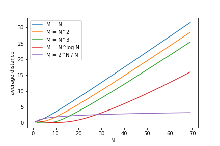
Figure 6: Average distances of different $N$ and $M$.

We can observe that even for $M=O(N^{\log N})$, the average distance is still growing linearly.

Appendix E Numerical Experiments for Rank-based DCM

In this section, we complement the results in Theorem 4 by additional numerical studies. Theorem 4 states that the random forest algorithm can recover the rank-based DCM with a single ranking when the training data is sampled uniformly. We will demonstrate numerically that the result still holds when the training data is not uniform. We also provide some examples showing that even though random forests may fail to recover the rankings exactly, the predicted probability is still quite accurate. Moreover, we demonstrate the insights that when the rank-based DCM consists of more than one ranks (customer types), the random forest may output a tree that “concatenates” multiple ranks.

E.1 Non-uniform Training Data

Consider $N=3$ products for the illustration purpose. Suppose customers prefer $1\succ 2\succ 3\succ 0$, where 0 denotes the outside option. Figure 7(a) illustrates the decision tree corresponding to the preference of the customers, where the splits are in the order of 1, 2, 3. We evaluate the performance of random forests by the number of correct splits until the first mistake is made. Notice that if the algorithm returns a tree that correctly splits the first $i$ cuts, then it can accurately predict a fraction of $1-1/2^{i}$ of total assortments. For example, if the splits are 1, 3, 2 in order, then the algorithm makes one correct split and accurately predicts a half of total assortments.

Now consider $N=10$ and $2^{N}=1024$ possible assortments (including the empty set). The parameter of random forests are $B=10,z=T,m=N,l=1$. We compare the performance of random forests in the following three sampling schemes:

1. Uniform: Each assortment is observed with equal probability $1/2^{N}$;

2. Non-uniform: The probability of observing each assortment follows a Dirichlet distribution with concentration parameters all equal to ones;

3. Different occurrences: generate probability $p_{i}$ for each product, where $p_{i}$ independently follows a normal distribution with mean 0.5 and standard deviation 0.15 so that $p_{i}$ falls into $[0,1]$ with high probability. We set $p_{i}=0$ if the random variable is negative and $p_{i}=1$ if it exceeds 1. In each assortment in the data, each product is included with probability $p_{i}$.

We test different sizes of training data $T\in[100,1000,10000]$. For each setup, we generate 100 independent datasets and inspect $B=10$ trees for each dataset. The mean and standard deviation of the correct splits are reported in Table 22.

$T$	Uniform	Non-uniform	Different occurrences
100	4.281 (0.951)	4.185 (0.922)	3.575 (1.372)
1000	7.715 (1.058)	7.370 (1.110)	6.369 (1.732)
10000	9.961 (0.256)	9.131 (0.986)	8.610 (2.145)

Table 22: The number of correct splits by random forests.

In general the uniform sampling has the best performance, but the algorithm is quite robust to other non-uniform sampling schemes.

E.2 Reconstruction of Decision Trees

From the numerical studies, we observe that some of the trees learned from the random forest may not have the some structure as the actual ranking. They nevertheless represent the same choice probabilities. To illustrate, consider $N=3$ and let the consumers’ ranking be represented by Figure 7(a). The random forest may learn a tree as shown in Figure 7(b) or 7(c), which represents the same DCM but with a different structure.

for tree=l sep+=.8cm,s sep+=.5cm,shape=rectangle, rounded corners, draw, align=center, top color=white, bottom color=gray!20 [Has product 1 [1,edge label=node[midway,left]Y ] [Has product 2,edge label=node[midway,right]N [2, edge label=node[midway,left]Y] [Has product 3, edge label=node[midway,right]N [3, edge label=node[midway,left]Y] [0, edge label=node[midway,right]N] ] ] ]

(a) The tree representing the preference list of consumers

for tree=l sep+=.8cm,s sep+=.5cm,shape=rectangle, rounded corners, draw, align=center, top color=white, bottom color=gray!20 [Has product 2 [Has product 1,edge label=node[midway,left]Y [1, edge label=node[midway,left]Y] [2, edge label=node[midway,right]N] ] [Has product 1,edge label=node[midway,right]N [1, edge label=node[midway,left]Y] [Has product 3, edge label=node[midway,right]N [3, edge label=node[midway,left]Y] [0, edge label=node[midway,right]N] ] ] ]

(b) A reconstructed tree having the same choice

for tree=l sep+=.8cm,s sep+=.5cm,shape=rectangle, rounded corners, draw, align=center, top color=white, bottom color=gray!20 [Has product 3 [Has product 1,edge label=node[midway,left]Y [1, edge label=node[midway,left]Y] [Has product 2, edge label=node[midway,right]N [2, edge label=node[midway,left]Y] [3, edge label=node[midway,right]N] ] ] [Has product 1,edge label=node[midway,right]N [1, edge label=node[midway,left]Y] [Has product 2, edge label=node[midway,right]N [2, edge label=node[midway,left]Y] [0, edge label=node[midway,right]N] ] ] ]

(c) A reconstructed tree having the same choice

Figure 7: Three possible trees representing the same choice.

E.3 Multiple Rankings

Next we study the case when customers are represented by a mixture of multiple rankings. More precisely, consider $N=5$ and two customer segments. Suppose 70% of customers are type one and have preference $1\succ 2\succ 3\succ 4\succ 5\succ 0$; the remaining 30% of customers are type two preferring $5\succ 4\succ 3\succ 2\succ 1\succ 0$. When $T=1000,B=10,z=T,m=N,l=1$, a number of trees learned by Algorithm 1 resemble the structure shown in Figure 8. There may be more than one chosen product in the leaf node explained in (2). For example, “1(5)” implies that most customers select product one in this leaf node, but some others purchase product 5. We can see that the main branch on the right looks like the preference list of type one. Meanwhile, some branches of the ranking of type two customers are attached to it. Random forests somehow merge the preferences of various segments into a single tree. This is a phenomenon commonly observed in our experiments and may shed light on the robust performance of random forests.

for tree=l sep+=.5cm,s sep+=.3cm,shape=rectangle, rounded corners, draw, align=center, top color=white, bottom color=gray!20 [Has 1 [Has 5,edge label=node[midway,left]Y [1(5), edge label=node[midway,left]Y] [Has 4, edge label=node[midway,right]N [1(4), edge label=node[midway,left]Y] [Has 3, edge label=node[midway,right]N [1(3), edge label=node[midway,left]Y] [Has 2, edge label=node[midway,right]N [1(2), edge label=node[midway,left]Y] [1, edge label=node[midway,right]N] ] ] ] ] [Has 2,edge label=node[midway,right]N [Has 5, edge label=node[midway,left]Y [2(5), edge label=node[midway,left]Y] [Has 4, edge label=node[midway,right]N [2(4), edge label=node[midway,left]Y] [Has 3, edge label=node[midway,right]N [2(3), edge label=node[midway,left]Y] [2, edge label=node[midway,right]N] ] ] ] [Has 3, edge label=node[midway,right]N [Has 5, edge label=node[midway,left]Y [3(5), edge label=node[midway,left]Y] [Has 4, edge label=node[midway,right]N [3(4), edge label=node[midway,left]Y] [3, edge label=node[midway,right]N] ] ] [Has 4, edge label=node[midway,right]N [Has 5, edge label=node[midway,left]Y [4(5), edge label=node[midway,left]Y] [4, edge label=node[midway,right]N] ] [Has 5, edge label=node[midway,right]N [5, edge label=node[midway,left]Y] [0, edge label=node[midway,right]N] ] ] ] ] ]

Figure 8: A tree output by random forests that merges two rankings.

Appendix F Numerical Examples for Product Importance

F.1 Synthetic Examples

Here we give an example of MDI (see Section 5.3 for details) under the rank-based DCM (with one ranking) and the MNL model.

Example 3.

Consider 10 products and data size $T=10000$. The assortment in training data is uniformly generated among non-empty subsets. We use $B=1000,m=\sqrt{N},l=50$ for the random forest algorithm. The ground-truth model is a single ranking: $1\succ 2\succ\ldots\succ 10$. The MDI is shown in Figure 9. We can observe that the MDI is decreasing in product indices.

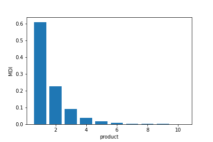
Figure 9: MDI of a single ranking when $N=10,T=10000$.

When the ground-truth model is MNL, we generate utilities $u_{i}$ from a uniform distribution on $[0,1]$ for each product. The attraction of product $i$ is defined as $a_{i}=\exp(u_{i})$ and the choice probability is $p(i,S)=a_{i}/\sum_{j\in S}a_{j}$. We show the attractions and MDI of random forests in Figure 10. It is clear that the MDI is highly correlated with attractions.

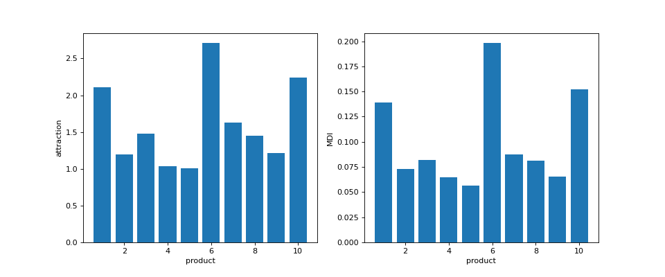
Figure 10: MDI of the MNL model when $N=10,T=10000$.

F.2 Hotel and IRI Datasets

We also calculate the MDI for the hotel and IRI datasets. Products with the highest MDI are listed in Tables 23 and 24. In the IRI dataset (Table 24), the products are represented by the vendor codes. MDI-insightsThe products with the highest MDI do not necessarily have high demand, but play an important role in customers’ decision process. Therefore, we recommend the firms to prioritize the experimentation of these products when optimizing over assortments or prices.

Hotel	Room type	MDI
Hotel 1	King Room 3	0.222
	Special Type Room 1	0.160
	Queen Room 2	0.100
	King Room 4	0.096
Hotel 2	2 Queen Beds Room 2 Smoking	0.279
	2 Queen Beds Room 1 Non-Smoking	0.202
	2 Queen Beds Room 2 Non-Smoking	0.157
	King Room 3 Non-Smoking	0.148
Hotel 3	King Room 1 Non-Smoking	0.523
	2 Double Beds Room 1 Non-Smoking	0.263
	King Room 3 Non-Smoking	0.081
	2 Double Beds Room 1 Smoking	0.049
Hotel 4	King Room 1 Non-Smoking	0.641
	2 Queen Beds Room 1 Non-Smoking	0.179
	2 Queen Beds Room 1 Smoking	0.100
	Suite 2 Non-Smoking	0.080
Hotel 5	King Room 2 Non-Smoking	0.496
	King Room 1 Non-Smoking	0.228
	2 Double Beds Room 1 Non-Smoking	0.085
	2 Double Beds Room 2 Non-Smoking	0.077

Table 23: Four room types with the highest MDI in each hotel.

Product Category	No.1 prod	MDI	No.2 prod	MDI	No.3 prod	MDI
Beer	87692	0.375	83820	0.364	78250	0.148
Blades	99998	0.302	52754	0.149	41058	0.140
Carbonated Beverages	73800	0.276	42200	0.178	71698	0.171
Cigarettes	710	0.322	90500	0.248	99998	0.170
Coffee	75101	0.210	11141	0.200	71038	0.162
Cold Cereal	42400	0.358	18627	0.175	21908	0.148
Deodorant	19045	0.315	9973	0.297	22600	0.150
Diapers	99998	0.424	48157	0.216	32913	0.206
Facial Tissue	63435	0.357	43032	0.296	99998	0.099
Frozen Dinners/Entrees	50100	0.334	17854	0.251	72655	0.234
Frozen Pizza	74653	0.234	19600	0.202	35300	0.180
Household Cleaners	35000	0.276	23400	0.260	25700	0.190
Hotdogs	75278	0.178	85331	0.168	46600	0.151
Laundry Detergent	45893	0.447	35000	0.186	72613	0.138
Margarine/Butter	96451	0.479	33100	0.202	34500	0.115
Mayonnaise	45200	0.248	52100	0.224	52500	0.172
Milk	99998	0.280	75457	0.269	41483	0.241
Mustard	71828	0.250	24000	0.235	70080	0.190
Paper Towels	43032	0.293	44096	0.216	30400	0.164
Peanut Butter	71018	0.321	45300	0.202	34000	0.117
Photo	74101	0.322	99998	0.280	41778	0.143
Razors	41058	0.350	99998	0.325	47400	0.197
Salt Snacks	41780	0.401	41262	0.284	72600	0.157
Shampoo	65632	0.350	71249	0.226	99998	0.142
Soup	41789	0.351	24000	0.332	50100	0.164
Spaghetti/Italian Sauce	72940	0.313	77644	0.254	6010	0.161
Sugar Substitutes	99998	0.191	19098	0.174	58312	0.137
Toilet Tissue	43032	0.416	44096	0.233	30400	0.205
Toothbrushes	70942	0.252	69055	0.216	416	0.140
Toothpaste	68305	0.376	77326	0.248	10310	0.164
Yogurt	21000	0.389	41148	0.171	53600	0.151

Table 24: Three product vendors with the highest MDI in each category of the IRI dataset.

Appendix G Additional Results for the IRI Dataset

In this section, we provide additional results for the IRI dataset when the top five and fifteen products are considered. The setup is described in Section 6.1.

Product category	#Data	#Unique assort	#Avg prod	RF	MNL	MC
Beer	10,440	8	2.88	0.3268 (0.0005)	0.3269 (0.0006)	0.3268 (0.0006)
Blades	1,085	10	3.10	0.3200 (0.0054)	0.3192 (0.0052)	0.3197 (0.0052)
Carbonated Beverages	71,114	4	3.75	0.3503 (0.0006)	0.3508 (0.0006)	0.3505 (0.0006)
Cigarettes	6,760	8	3.50	0.2916 (0.0023)	0.2916 (0.0024)	0.2916 (0.0024)
Coffee	8,135	8	3.50	0.3396 (0.0012)	0.3405 (0.0012)	0.3400 (0.0012)
Cold Cereal	30,369	4	4.00	0.3324 (0.0004)	0.3324 (0.0004)	0.3324 (0.0004)
Deodorant	2,775	4	3.75	0.3429 (0.0005)	0.3430 (0.0005)	0.3430 (0.0005)
Diapers	1,528	6	3.17	0.3585 (0.0030)	0.3590 (0.0022)	0.3590 (0.0024)
Facial Tissue	8,956	9	3.12	0.3389 (0.0006)	0.3422 (0.0009)	0.3410 (0.0007)
Frozen Dinners/Entrees	48,349	6	3.83	0.3298 (0.0004)	0.3303 (0.0005)	0.3300 (0.0004)
Frozen Pizza	16,263	14	3.43	0.3471 (0.0005)	0.3491 (0.0004)	0.3478 (0.0004)
Household Cleaners	6,403	4	3.50	0.3272 (0.0025)	0.3272 (0.0024)	0.3272 (0.0024)
Hotdogs	7,281	13	3.08	0.3489 (0.0017)	0.3511 (0.0016)	0.3498 (0.0019)
Laundry Detergent	7,854	11	3.36	0.3319 (0.0021)	0.3343 (0.0018)	0.3333 (0.0018)
Margarine/Butter	9,534	5	3.80	0.3428 (0.0005)	0.3431 (0.0004)	0.3429 (0.0004)
Mayonnaise	4,380	7	2.71	0.3552 (0.0010)	0.3567 (0.0008)	0.3553 (0.0009)
Milk	56,849	12	3.25	0.2641 (0.0012)	0.2645 (0.0011)	0.2643 (0.0012)
Mustard	5,354	7	3.29	0.3348 (0.0007)	0.3353 (0.0007)	0.3350 (0.0007)
Paper Towels	9,520	8	3.63	0.3258 (0.0012)	0.3260 (0.0013)	0.3258 (0.0013)
Peanut Butter	4,985	9	3.44	0.3321 (0.0012)	0.3332 (0.0008)	0.3326 (0.0011)
Photography supplies	189	17	2.88	0.3526 (0.0117)	0.3526 (0.0111)	0.3542 (0.0100)
Razors	111	8	2.50	0.2942 (0.0567)	0.2957 (0.0458)	0.2992 (0.0444)
Salt Snacks	44,975	7	3.57	0.3140 (0.0009)	0.3152 (0.0009)	0.3147 (0.0008)
Shampoo	3,353	8	3.38	0.3391 (0.0011)	0.3390 (0.0010)	0.3390 (0.0010)
Soup	68,049	5	4.20	0.3346 (0.0003)	0.3355 (0.0003)	0.3350 (0.0003)
Spaghetti/Italian Sauce	12,377	7	3.43	0.3369 (0.0008)	0.3371 (0.0008)	0.3369 (0.0008)
Sugar Substitutes	1,269	9	3.44	0.3276 (0.0050)	0.3274 (0.0053)	0.3277 (0.0053)
Toilet Tissue	11,154	9	3.44	0.3421 (0.0002)	0.3428 (0.0002)	0.3424 (0.0001)
Toothbrushes	2,562	12	3.25	0.3415 (0.0010)	0.3415 (0.0012)	0.3414 (0.0011)
Toothpaste	4,258	6	3.50	0.3230 (0.0016)	0.3229 (0.0017)	0.3229 (0.0017)
Yogurt	61,671	11	3.18	0.3341 (0.0011)	0.3383 (0.0011)	0.3369 (0.0011)

Table 25: The summary statistics (the data size, the number of unique assortments in the data, and the average number of products in an assortment) of the IRI dataset after preprocessing and the average and standard deviation of the out-of-sample RMSE (6) for each category when considering the top 5 products.

Product category	#Data	#Unique assort	#Avg prod	RF	MNL	MC
Beer	10,441	234	10.13	0.2294 (0.0010)	0.2303 (0.0009)	0.2302 (0.0010)
Blades	1,085	56	5.46	0.3092 (0.0036)	0.3074 (0.0040)	0.3077 (0.0041)
Carbonated Beverages	71,114	229	7.83	0.2733 (0.0003)	0.2763 (0.0004)	0.2759 (0.0005)
Cigarettes	6,760	179	6.86	0.2521 (0.0015)	0.2530 (0.0020)	0.2528 (0.0017)
Coffee	8,135	269	9.08	0.2619 (0.0011)	0.2669 (0.0008)	0.2656 (0.0009)
Cold Cereal	30,369	325	10.52	0.2375 (0.0005)	0.2387 (0.0004)	0.2386 (0.0004)
Deodorant	2,775	227	10.41	0.2439 (0.0008)	0.2436 (0.0006)	0.2435 (0.0006)
Diapers	1,528	13	3.85	0.3581 (0.0027)	0.3583 (0.0022)	0.3584 (0.0025)
Facial Tissue	8,956	63	4.89	0.3238 (0.0010)	0.3306 (0.0012)	0.3290 (0.0011)
Frozen Dinners/Entrees	48,349	163	11.13	0.2282 (0.0003)	0.2318 (0.0002)	0.2311 (0.0002)
Frozen Pizza	16,263	317	8.25	0.2680 (0.0008)	0.2742 (0.0002)	0.2726 (0.0003)
Household Cleaners	6,403	93	11.78	0.2346 (0.0005)	0.2347 (0.0004)	0.2346 (0.0004)
Hotdogs	7,281	259	7.61	0.2764 (0.0017)	0.2863 (0.0006)	0.2837 (0.0010)
Laundry Detergent	7,854	158	7.81	0.2589 (0.0020)	0.2717 (0.0019)	0.2689 (0.0017)
Margarine/Butter	9,534	89	9.34	0.2733 (0.0003)	0.2745 (0.0003)	0.2740 (0.0003)
Mayonnaise	4,380	263	6.79	0.2912 (0.0022)	0.2958 (0.0006)	0.2938 (0.0011)
Milk	56,849	99	6.47	0.2318 (0.0011)	0.2379 (0.0013)	0.2362 (0.0014)
Mustard	5,354	410	9.84	0.2476 (0.0009)	0.2492 (0.0006)	0.2487 (0.0005)
Paper Towels	9,520	80	6.66	0.2870 (0.0009)	0.2903 (0.0009)	0.2894 (0.0008)
Peanut Butter	4,985	166	7.10	0.2896 (0.0019)	0.2986 (0.0012)	0.2970 (0.0014)
Photography supplies	189	37	3.43	0.3416 (0.0094)	0.3455 (0.0085)	0.3444 (0.0086)
Razors	111	10	2.60	0.3269 (0.0334)	0.3294 (0.0251)	0.3323 (0.0218)
Salt Snacks	44,975	170	7.89	0.2463 (0.0012)	0.2487 (0.0011)	0.2481 (0.0012)
Shampoo	3,354	219	10.96	0.2387 (0.0006)	0.2380 (0.0007)	0.2380 (0.0007)
Soup	68,049	199	10.82	0.2258 (0.0004)	0.2330 (0.0003)	0.2321 (0.0003)
Spaghetti/Italian Sauce	12,377	207	9.43	0.2532 (0.0010)	0.2568 (0.0008)	0.2563 (0.0007)
Sugar Substitutes	1,269	126	6.13	0.3060 (0.0050)	0.3049 (0.0051)	0.3046 (0.0050)
Toilet Tissue	11,154	67	7.21	0.2971 (0.0006)	0.3022 (0.0003)	0.3011 (0.0004)
Toothbrushes	2,562	280	10.49	0.2431 (0.0010)	0.2436 (0.0004)	0.2434 (0.0004)
Toothpaste	4,258	550	9.64	0.2360 (0.0013)	0.2377 (0.0010)	0.2377 (0.0011)
Yogurt	61,671	121	6.36	0.2730 (0.0011)	0.2803 (0.0009)	0.2782 (0.0009)

Table 26: The summary statistics (the data size, the number of unique assortments in the data, and the average number of products in an assortment) of the IRI dataset after preprocessing and the average and standard deviation of the out-of-sample RMSE (6) for each category when considering the top 15 products.

References

- Anderson et al. (1992) Anderson, S. P., A. De Palma, and J.-F. Thisse (1992). Discrete choice theory of product differentiation. MIT press.
- Aouad et al. (2019) Aouad, A., A. N. Elmachtoub, K. J. Ferreira, and R. McNellis (2019). Market segmentation trees. arXiv preprint arXiv:1906.01174.
- Ariely (2008) Ariely, D. (2008). Predictably irrational. Harper Audio.
- Berbeglia (2019) Berbeglia, G. (2019). The generalized stochastic preference choice model. Working paper.
- Berbeglia et al. (2018) Berbeglia, G., A. Garassino, and G. Vulcano (2018). A comparative empirical study of discrete choice models in retail operations. Working paper.
- Bernstein et al. (2018) Bernstein, F., S. Modaresi, and D. Sauré (2018). A dynamic clustering approach to data-driven assortment personalization. Management Science 65(5), 2095–2115.
- Biau and Scornet (2016) Biau, G. and E. Scornet (2016). A random forest guided tour. Test 25(2), 197–227.
- Blanchet et al. (2016) Blanchet, J., G. Gallego, and V. Goyal (2016). A markov chain approximation to choice modeling. Operations Research 64(4), 886–905.
- Block et al. (1959) Block, H. D., J. Marschak, et al. (1959). Random orderings and stochastic theories of response. Technical report, Cowles Foundation for Research in Economics, Yale University.
- Bodea et al. (2009) Bodea, T., M. Ferguson, and L. Garrow (2009). Data set—choice-based revenue management: Data from a major hotel chain. Manufacturing & Service Operations Management 11(2), 356–361.
- Breiman (2001) Breiman, L. (2001). Random forests. Machine learning 45(1), 5–32.
- Bronnenberg et al. (2008) Bronnenberg, B. J., M. W. Kruger, and C. F. Mela (2008). Database paper—the iri marketing data set. Marketing science 27(4), 745–748.
- Chen and Mišić (2019) Chen, Y.-C. and V. V. Mišić (2019). Decision forest: A nonparametric approach to modeling irrational choice. Working paper.
- Cohen et al. (1997) Cohen, G., I. Honkala, S. Litsyn, and A. Lobstein (1997). Covering codes. Elsevier.
- Devroye et al. (2013) Devroye, L., L. Györfi, and G. Lugosi (2013). A probabilistic theory of pattern recognition, Volume 31. Springer Science & Business Media.
- Farias et al. (2013) Farias, V. F., S. Jagabathula, and D. Shah (2013). A nonparametric approach to modeling choice with limited data. Management science 59(2), 305–322.
- Feng et al. (2017) Feng, G., X. Li, and Z. Wang (2017). On the relation between several discrete choice models. Operations research 65(6), 1516–1525.
- Flores et al. (2017) Flores, A., G. Berbeglia, and P. Van Hentenryck (2017). Assortment and price optimization under the two-stage luce model. Working paper.
- Györfi et al. (2006) Györfi, L., M. Kohler, A. Krzyzak, and H. Walk (2006). A distribution-free theory of nonparametric regression. Springer Science & Business Media.
- Hastie et al. (2009) Hastie, T., R. Tibshirani, and J. Friedman (2009). The Elements of Statistical Learning: Data Mining, Inference, and Prediction. Springer series in statistics. Springer.
- Huber et al. (1982) Huber, J., J. W. Payne, and C. Puto (1982). Adding asymmetrically dominated alternatives: Violations of regularity and the similarity hypothesis. Journal of consumer research 9(1), 90–98.
- Jagabathula and Rusmevichientong (2018) Jagabathula, S. and P. Rusmevichientong (2018). The limit of rationality in choice modeling: Formulation, computation, and implications. Management Science 65(5), 2196–2215.
- Jagabathula et al. (2018) Jagabathula, S., L. Subramanian, and A. Venkataraman (2018). A model-based embedding technique for segmenting customers. Operations Research 66(5), 1247–1267.
- Jagabathula et al. (2019) Jagabathula, S., L. Subramanian, and A. Venkataraman (2019). A conditional gradient approach for nonparametric estimation of mixing distributions. Management Science.
- Liaw and Wiener (2002) Liaw, A. and M. Wiener (2002). Classification and regression by randomforest. R News 2(3), 18–22.
- Lin and Jeon (2006) Lin, Y. and Y. Jeon (2006). Random forests and adaptive nearest neighbors. Journal of the American Statistical Association 101(474), 578–590.
- McFadden (1973) McFadden, D. (1973). Conditional logit analysis of qualitative choice behaviour. In P. Zarembka (Ed.), Frontiers in Econometrics, pp. 105–142. New York, NY, USA: Academic Press New York.
- Mišić (2020) Mišić, V. V. (2020). Optimization of tree ensembles. Operations Research 68(5), 1605–1624.
- Natarajan et al. (2009) Natarajan, K., M. Song, and C.-P. Teo (2009). Persistency model and its applications in choice modeling. Management Science 55(3), 453–469.
- Östergård and Kaikkonen (1998) Östergård, P. R. and M. K. Kaikkonen (1998). New upper bounds for binary covering codes. Discrete Mathematics 178(1-3), 165–179.
- Pedregosa et al. (2011) Pedregosa, F., G. Varoquaux, A. Gramfort, V. Michel, B. Thirion, O. Grisel, M. Blondel, P. Prettenhofer, R. Weiss, V. Dubourg, J. Vanderplas, A. Passos, D. Cournapeau, M. Brucher, M. Perrot, and E. Duchesnay (2011). Scikit-learn: Machine Learning in Python . Journal of Machine Learning Research 12, 2825–2830.
- Russo and Dosher (1983) Russo, J. E. and B. A. Dosher (1983). Strategies for multiattribute binary choice. Journal of Experimental Psychology: Learning, Memory, and Cognition 9(4), 676.
- Scornet et al. (2015) Scornet, E., G. Biau, J.-P. Vert, et al. (2015). Consistency of random forests. The Annals of Statistics 43(4), 1716–1741.
- Simonson and Tversky (1992) Simonson, I. and A. Tversky (1992). Choice in context: Tradeoff contrast and extremeness aversion. Journal of marketing research 29(3), 281–295.
- Şimşek and Topaloglu (2018) Şimşek, A. S. and H. Topaloglu (2018). An expectation-maximization algorithm to estimate the parameters of the markov chain choice model. Operations Research 66(3), 748–760.
- Train (2009) Train, K. E. (2009). Discrete choice methods with simulation. Cambridge university press.
- van Ryzin and Vulcano (2014) van Ryzin, G. and G. Vulcano (2014). A market discovery algorithm to estimate a general class of nonparametric choice models. Management Science 61(2), 281–300.
- van Ryzin and Vulcano (2017) van Ryzin, G. and G. Vulcano (2017). An expectation-maximization method to estimate a rank-based choice model of demand. Operations Research 65(2), 396–407.
- Wager (2014) Wager, S. (2014). Asymptotic theory for random forests. arXiv preprint arXiv:1405.0352.
- Wager and Athey (2018) Wager, S. and S. Athey (2018). Estimation and inference of heterogeneous treatment effects using random forests. Journal of the American Statistical Association 113(523), 1228–1242.
- Weitzman (1979) Weitzman, M. L. (1979). Optimal search for the best alternative. Econometrica, 641–654.
- Williams (1977) Williams, H. C. (1977). On the formation of travel demand models and economic evaluation measures of user benefit. Environment and planning A 9(3), 285–344.