Simultaneous Semantic Segmentation and
Outlier Detection in Presence of Domain Shift

Abstract

Recent success on realistic road driving datasets has increased interest in exploring robust performance in real-world applications. One of the major unsolved problems is to identify image content which can not be reliably recognized with a given inference engine. We therefore study approaches to recover a dense outlier map alongside the primary task with a single forward pass, by relying on shared convolutional features. We consider semantic segmentation as the primary task and perform extensive validation on WildDash val (inliers), LSUN val (outliers), and pasted objects from Pascal VOC 2007 (outliers). We achieve the best validation performance by training to discriminate inliers from pasted ImageNet-1k content, even though ImageNet-1k contains many road-driving pixels, and, at least nominally, fails to account for the full diversity of the visual world. The proposed two-head model performs comparably to the C-way multi-class model trained to predict uniform distribution in outliers, while outperforming several other validated approaches. We evaluate our best two models on the WildDash test dataset and set a new state of the art on the WildDash benchmark.

1 Introduction

Early computer vision approaches focused on producing decent performance on small datasets. This often posed overwhelming difficulties, so researchers seldom quantified the prediction confidence. An important milestone was reached when generalization was achieved on realistic datasets such as Pascal VOC [13], CamVid [5], KITTI [14], and Cityscapes [9]. These datasets assume closed-world evaluation [39] in which the training and test subsets are sampled from the same distribution. Such setup has been able to provide a fast feedback on novel approaches due to good alignment with the machine learning paradigm. This further accelerated development and led us to the current state of research where all these datasets are mostly solved, at least in the strongly supervised setup.

Recent datasets further raise the bar by increasing the number of classes and image diversity. However, despite this increased complexity, the Vistas [36] dataset is still an insufficient proxy for real-life operation even in a very restricted scenario such as road driving. New classes like bike racks and ground animals were added, however many important classes from non-typical or worst-case images are still absent. These classes include persons in non-standard poses, crashed vehicles, rubble, fallen trees etc. Additionally, real-life images may be affected by particular image acquisition faults including hardware defects, covered lens etc. This suggests that foreseeing every possible situation may be an elusive goal, and that our algorithms should be designed to recognize image regions which are foreign to the training distribution.

The described deficiencies emphasize the need for a more robust approach to dataset design. First, an ideal dataset should identify and target a set of explicit hazards for the particular domain [47]. Second (and more important), an ideal dataset should endorse open-set recognition paradigm [39] in order to promote detection of unforeseen hazards. Consequently, the validation (val) and test subsets should contain various degrees of domain shift with respect to the training distribution. This should include moderate domain shift factors (e.g. adverse weather, exotic locations), exceptional situations (e.g. accidents, poor visibility, defects) and outright outliers (objects and entire images from other domains). We argue that the WildDash dataset [47] represents a step in the right direction, although further development would be welcome, especially in the direction of enlarging the negative part of the test dataset [3]. Models trained for open-set evaluation can not be required to predict an exact visual class in outlier pixels. Instead, it should suffice that the outliers are recognized, as illustrated in Fig. 1 on an image from the WildDash dataset.

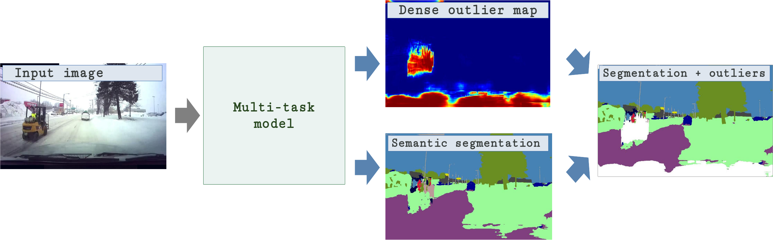
Figure 1: The proposed approach for simultaneous semantic segmentation and outlier detection. Our multi-task model predicts i) a dense outlier map, and ii) a semantic map with respect to the 19 Cityscapes classes. The two maps are merged to obtain the final outlier-aware semantic predictions. Our model recognizes outlier pixels (white) on two objects which are foreign to Cityscapes: the ego-vehicle and the yellow forklift.

This paper addresses simultaneous semantic segmentation and open-set outlier detection. We train our models on inlier images from two road-driving datasets: Cityscapes [9] and Vistas [36]. We consider several outlier detection approaches from the literature [20, 2, 21] and validate their performance on WildDash val (inliers), LSUN val [45] (outliers), and pasted objects from Pascal VOC 2007 (outliers). Our main hypotheses are i) that training with noisy negatives from a very large and diverse dataset such as ImageNet-1k [10] can improve outlier detection, and ii) that discriminative outlier detection and semantic segmentation can share features without significant deterioration of either task. We confirm both hypotheses by re-training our best models on WildDash val, Vistas and ImageNet-1k, and evaluating performance on the WildDash benchmark.

2 Related Work

Previous approaches to outlier detection in image data are very diverse. These approaches are based on analyzing prediction uncertainty, evaluating generative models, or exploiting a broad secondary dataset which contains both outliers and inliers. Our approach is also related to multi-task models and previous work which explores the dataset quality and dataset bias.

2.1 Estimating Uncertainty (or Confidence) of the Predictions

Prediction confidence can be expressed as the probability of the winning class or max-softmax for short [20]. This is useful in image-wide prediction of outliers, although max-softmax must be calibrated [16] before being interpreted as $P(\mathrm{inlier}|\mathbf{x})$. The ODIN approach [32] improves on [20] by pre-processing input images with a well-tempered perturbation aimed at increasing the max-softmax activation. These approaches are handy since they require no additional training.

Some approaches model the uncertainty with a separate head which learns either prediction uncertainty [24, 29] or confidence [11]. Such training is able to recognize examples which are hard to classify due to insufficient or inconsistent labels, but is unable to deal with real outliers.

A principled information-theoretic approach expresses the prediction uncertainty as mutual information between the posterior parameter distribution and the particular prediction [41]. In practice, the required expectations are estimated with Monte Carlo (MC) dropout [24]. Better results have been achieved with explicit ensembles of independently trained models [29]. However, both approaches require many forward passes and thus preclude real-time operation.

Prediction uncertainty can also be expressed by evaluating per-class generative models of latent features [31]. However, this idea is not easily adaptable for dense prediction in which latent features typically correspond to many classes due to subsampling and dense labelling. Another approach would be to fit a generative model to the training dataset and to evaluate the likelihood of a given sample. Unfortunately, this is very hard to achieve with image data [35].

2.2 Training with Negative Data

Our approach is most related to three recent approaches which train outlier detection by exploiting a diverse negative dataset [42]. The approach called outlier exposure (OE) [21] processes the negative data by optimizing cross entropy between the predictions and the uniform distribution. Outlier detection has also been formulated as binary classification [2] trained to differentiate inliers from the negative dataset. A related approach [43] partitions the training data into K folds and trains an ensemble of K leave-one-fold-out classifiers. However, this requires K forward passes. while data partitioning may not be straight-forward.

Negative training samples can also be produced by a GAN generator [15]. Unfortunately, existing works [30, 38] have been designed for image-wide prediction in small images. Their adaptation to dense prediction on Cityscapes resolution would not be straight-forward [4].

Soundness of training with negative data has been challenged by [40] who report under-average results for this approach. However, their experiments average results over all negative datasets (including MNIST), while we advocate for a very diverse negative dataset such as ImageNet.

2.3 Multi-task Training and Dataset Design

Multi-task models attach several prediction heads to shared features [7]. Each prediction head has a distinct loss. The total loss is usually expressed as a weighted sum [37] and optimized in an end-to-end fashion. Feature sharing brings important advantages such as cross-task enrichment of training data [1] and faster evaluation. Examples of successful multi-task models include combining depth, surface normals and semantic segmentation [12], as well as combining classification, bounding box prediction and per-class instance-level segmentation [17]. A map of task compatibility with respect to knowledge transfer [46] suggests that many tasks are suitable for multi-task training.

Dataset quality is as a very important issue in computer vision research. Diverse negative datasets have been used to reduce false positives in several computer vision tasks for a very long time [42]. A methodology for analyzing the quality of road-driving datasets has been proposed in [48]. The WildDash dataset [47] proposes a very diverse validation dataset and the first semantic segmentation benchmark with open-set evaluation [39].

3 Simultaneous Segmentation and Outlier Detection

Our method combines two distinct tasks: outlier detection and semantic segmentation, as shown in Fig. 1. We prefer to rely on shared features in order to promote fast inference and synergy between tasks [1]. We assume that a large, diverse and noisy negative dataset is available for training purposes [21, 2].

3.1 Dense Feature Extractor

Our models are based on a dense feature extractor with lateral connections [26]. The processing starts with a DenseNet [22] or ResNet [19] backbone, proceeds with spatial pyramid pooling (SPP) [18, 49] and concludes with ladder-style upsampling [26, 33]. The upsampling path consists of three upsampling blocks (U1-U3) which blend low resolution features from the previous upsampling stage with high resolution features from the backbone. We speed-up and regularize the learning with three auxiliary classification losses (cf. Fig. 2). These losses have soft targets corresponding to ground truth distribution across the corresponding window at full resolution [27].

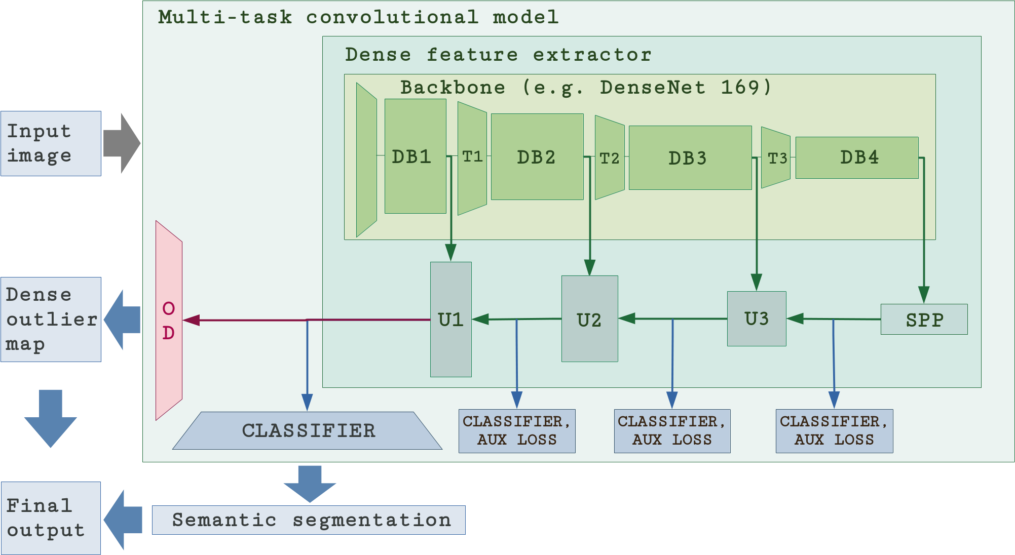
Figure 2: The proposed two-head model: the classification head recovers semantic segmentation while the outlier detection head identifies pixels where semantic segmentation may be wrong. The output is produced by combining these two dense prediction maps.

3.2 Dense Outlier Detection

There are four distinct approaches to formulate simultaneous semantic segmentation and dense outlier detection over shared features. The C-way multi-class approach attaches the standard classification head to the dense feature extractor (C denotes the number of inlier classes). The inlier probability is formulated as max-softmax. If a negative set is available, this approach can be trained to emit low max-softmax in outliers by supplying a modulated cross entropy loss term towards uniform distribution [30, 21]. The modulation factor $\lambda_{\textrm{KL}}$ is a hyper-parameter. Unfortunately, training on outliers may compromise classification accuracy and generate false positive outliers at semantic borders.

The C-way multi-label approach has C sigmoid heads. The final prediction is the class with maximum probability max-$\sigma$, whereas the inlier probability is formulated as max-$\sigma$. Unfortunately, this formulation fails to address the competition between classes, which again compromises classification accuracy.

The C+1-way multi-class approach includes outliers as the C+1-th class, whereas the inlier probability is a 2-way softmax between the max-logit over inlier classes and the outlier logit. To account for class disbalance we modulate the loss due to outliers with $\lambda_{\textrm{C+1}}$. Nevertheless, this loss affects inlier classification weights, which may be harmful when the negatives are noisy (as in our case).

Finally, the two-head approach complements the C-way classification head with a head which directly predicts the outlier probability as illustrated in Fig. 2. The classification head is trained on inliers while the outlier detection head is trained both on inliers and outliers. The outlier detection head uses the standard cross entropy loss modulated with hyper-parameter $\lambda_{\textrm{TH}}$. We combine the resulting prediction maps to obtain semantic segmentation into C+1 classes. The outlier detection head overrides the classification head whenever the outlier probability is greater than a threshold. Thus, the classification head is unaffected by the negative data, which provides hope to preserve the baseline semantic segmentation accuracy even when training on extremely large negative datasets.

3.3 Resistance to noisy outlier labels and sensitivity to negative objects in positive context

Training outlier detection on a diverse negative dataset has to confront noise in negative training data. For example, our negative dataset, ImageNet-1k, contains several classes (e.g. cab, streetcar) which are part of the Cityscapes ontology. Additionally, several stuff classes from Cityscapes (e.g. building, terrain) occur in ImageNet-1k backgrounds. Nevertheless, these pixels are vastly outnumbered by true inliers. This is especially the case when the training only considers the bounding box of the object which defines the ImageNet-1k class.

We address this issue by training our models on mixed batches with approximately equal share of inlier and negative images. Thus, we perform many inlier epochs during one negative epoch, since our negative training dataset is much larger than the inlier ones. The proposed batch formation procedure prevents occasional inliers from negative images to significantly affect the training. Additionally, it also favours stable development of batchnorm statistics. Hence, the proposed training approach stands a fair chance to succeed.

We promote detection of outlier objects in inlier context by pasting negative content into inlier training images. We first resize the negative image to 5% of the inlier image, and then paste it at random. We perform this before the cropping, so some crops may contain only inlier pixels. Unlike [3], we do not use the Cityscapes ignore class since it contains many inliers.

4 Experiments

We train most models on Vistas inliers [36] by mapping original labels to Cityscapes [9] classes. In some experiments we also use Cityscapes inliers to improve results and explore influence of the domain shift. We train all applicable models on outliers from two variants of ImageNet-1k: the full dataset (ImageNet-1k-full) and the subset in which bounding box annotations are available (ImageNet-1k-bb). In the latter case we use only the bounding box for training on negative images (the remaining pixels are ignored) and pasting into positive images.

We validate semantic segmentation by measuring mIoU on WildDash val separately from outlier detection. We validate outlier detection by measuring pixel level average precision (AP) in two different setups: i) entire images are either negative or positive, and ii) appearance of negative objects in positive context. The former setup consists of many assays across WildDash val and random subsets of LSUN images. The LSUN subsets are dimensioned so that the numbers of pixels in LSUN and WildDash val are approximately equal. Our experiments report mean and standard deviation of the detection AP across 50 assays. The latter setup involves WildDash val images with pasted Pascal animals. We select animals which take up at least 1% of the WildDash resolution, and paste them at random in each WildDash image.

We normalize all images with ImageNet mean and variance, and resize them so that the shorter side is 512 pixels. We form training batches with random 512$\times$512 crops which we jitter with horizontal flipping. We set the auxiliary loss weight to 0.4 and the classifier loss weight to 0.6. We set $\lambda_{\textrm{KL}}$=0.2, $\lambda_{\textrm{C+1}}$=0.05, and $\lambda_{\textrm{TH}}$=0.2. We use the standard Adam optimizer and divide the learning rate of pretrained parameters by 4. All our models are trained throughout 75 Vistas epochs, which corresponds to 2 epochs of ImageNet-1k-full, or 5 epochs of ImageNet-1k-bb. We detect outliers by thresholding inlier probability at $p_{\textrm{IP}}=0.5$. Our models produce a dense index map for C Cityscapes classes and 1 void class. We obtain predictions at the benchmark resolution by bilinear upsampling.

We perform ODIN inference as follows. First, we perform the forward pass and the backward pass with respect to the max-softmax activation (we use temperature T=10). Then we determine the max-softmax gradient with respect to pixels. We determine the perturbation by multiplying the sign of the gradient with $\varepsilon$=0.001. Finally, we perturb the normalized input image, perform another forward pass and detect outliers according to the max-softmax criterion.

4.1 Evaluation on the WildDash Benchmark

Table 1 presents our results on the WildDash semantic segmentation benchmark, and compares them to other submissions with accompanying publications.

Table 1: Evaluation of the semantic segmentation models on WildDash bench

	Meta Avg	Classic				Negative
Model	mIoU	mIoU	iIoU	mIoU	iIoU	mIoU
	cla	cla	cla	cat	cat	cla
APMoE_seg_ROB [25]	22.2	22.5	12.6	48.1	35.2	22.8
DRN_MPC [44]	28.3	29.1	13.9	49.2	29.2	15.9
DeepLabv3+_CS [8]	30.6	34.2	24.6	49.0	38.6	15.7
LDN2_ROB [28]	32.1	34.4	30.7	56.6	47.6	29.9
MapillaryAI_ROB [6]	38.9	41.3	38.0	60.5	57.6	25.0
AHiSS_ROB [34]	39.0	41.0	32.2	53.9	39.3	43.6
LDN_BIN (ours, two-head)	41.8	43.8	37.3	58.6	53.3	54.3
LDN_OE (ours, C$\times$ multi-class)	42.7	43.3	31.9	60.7	50.3	52.8

Our two models use the same backbone (DenseNet-169 [22]) and different outlier detectors. The LDN_OE model has a single C-way multi-class head. The LDN_BIN model has two heads as shown in Figure 2. Both models have been trained on Vistas train, Cityscapes train, and WildDash val (inliers), as well as on ImageNet-1k-bb with pasting (outliers). Our models significantly outperform all previous submissions on negative images, while also achieving the highest meta average mIoU (the principal benchmark metric) and the highest mIoU for classic images. We achieve the second-best iIoU score for classic images, which indicates underperformance on small objects. This is likely due to the fact that we train and evaluate our models on half resolution images.

4.2 Validation of Dense Outlier Detection Approaches

Table 9 compares various approaches for dense outlier detection. All models are based on DenseNet-169, and trained on Vistas (inliers). The first section shows the results of a C-way multi-class model trained without outliers, where outliers are detected with max-softmax [20] and ODIN + max-softmax [32]. We note that ODIN slightly improves the results across all experiments.

Table 2: Validation of dense outlier detection approaches. WD denotes WildDash val.

Model	ImageNet	AP WD-LSUN	AP WD-Pascal	mIoU WD
C$\times$ multi-class	✗	$55.65\pm 0.80$	6.01	49.07
C$\times$ multi-class, ODIN	✗	$55.98\pm 0.77$	6.92	49.77
C+1$\times$ multi-class	✓	$98.92\pm 0.06$	33.59	45.60
C$\times$ multi-label	✓	$98.75\pm 0.07$	57.31	42.72
C$\times$ multi-class	✓	$\textbf{99.49}\pm\textbf{0.04}$	41.72	46.69
two heads	✓	$99.25\pm 0.04$	46.83	47.37

The second section of the table shows the four dense outlier detection approaches (cf. Section 3) which we also train on ImageNet-1k-bb with pasting (outliers). Columns 3 and 4 clearly show that training with noisy and diverse negatives significantly improves outlier detection. However, we also note a reduction of the segmentation score as shown in the column 5. This reduction is lowest for the C-way multi-class model and the two-head model, which we analyze next.

The two-head model is slightly worse in discriminating WildDash val from LSUN, which indicates that it is more sensitive to domain shift between Vistas train and WildDash val. On the other hand, the two-head model achieves better inlier segmentation (0.7 pp, column 5), and much better outlier detection on Pascal animals (5 pp, column 4). A closer inspection shows that these advantages occur since the single-head C-way approach generates many false positive outlier detections at semantic borders due to lower max-softmax.

The C+1-way multi-class model performs the worst out of all models trained with noisy outliers. The sigmoid model performs well on outlier detection but underperforms on inlier segmentation.

4.3 Validation of Dense Feature Extractor Backbones

Table 3 explores influence of different backbones to the performance of our two-head model. We experiment with ResNets and DenseNets of varying depths. The upsampling blocks are connected with the first three DenseNet blocks, as shown in Fig. 2. In the ResNet case, the upsampling blocks are connected with the last addition at the corresponding subsampling level. We train on Vistas (inliers) and ImageNet-1k-bb with pasting (outliers).

Table 3: Validation of backbones for the two-head model. WD denotes WildDash val.

Backbone	AP WD-LSUN	AP WD-Pascal	mIoU WD
DenseNet-121	$99.05\pm 0.03$	55.84	44.75
DenseNet-169	$\textbf{99.25}\pm\textbf{0.04}$	46.83	47.37
DenseNet-201	$98.34\pm 0.07$	36.88	47.59
ResNet-34	$97.19\pm 0.07$	47.24	45.17
ResNet-50	$99.10\pm 0.04$	56.18	41.65
ResNet-101	$98.96\pm 0.06$	52.02	43.67

All models achieve very good outlier detection in negative images. There appears to be a trade-off between detection of outliers at negative objects and semantic segmentation accuracy. We opt for better semantic segmentation results since WildDash test does not have negative objects in positive context. We therefore use the DenseNet-169 backbone in most other experiments due to a very good overall performance.

4.4 Influence of the Training Data

Table 4 explores the influence of inlier training data to the model performance. All experiments involve the two-head model based on DenseNet-169, which was trained on outliers from ImageNet-1k-bb with pasting.

Table 4: Influence of the inlier training dataset to the performance of the two-head model with the DenseNet-169 backbone. WD denotes WildDash val.

Inlier training dataset	AP WD-LSUN	AP WD-Pascal	mIoU WD
Cityscapes	$66.57\pm 0.86$	13.85	11.12
Vistas	$99.25\pm 0.04$	46.83	47.17
Cityscapes, Vistas	$\textbf{99.29}\pm\textbf{0.03}$	53.68	47.78

The results suggest that there is a very large domain shift between Cityscapes and WildDash val. Training on inliers from Cityscapes leads to very low AP scores, which indicates that many WildDash val pixels are predicted as outliers with respect to Cityscapes. This suggests that Cityscapes is not an appropriate training dataset for real-world applications. Training on inliers from Vistas leads to much better results which is likely due to greater variety with respect to camera, time of day, weather, resolution etc. The best results across the board have been achieved when both inlier datasets are used for training.

Table 5 explores the impact of negative training data. All experiments feature the two-head model with DenseNet-169 trained on inliers from Vistas.

Table 5: Influence of the outlier training dataset to the performance of our two-head model with the DenseNet-169 backbone. WD denotes WildDash val.

Outlier training dataset	outlier pasting	AP WD-Pascal	mIoU WD
ImageNet-1k-full	no	2.94	43.13
ImageNet-1k-full	yes	45.96	43.68
ImageNet-1k-bb	yes	46.83	47.17

The table shows that training with pasted negatives greatly improves outlier detection on negative objects. It is intuitively clear that a model which never sees a border between inliers and outliers during training does not stand a chance to accurately locate such borders during inference.

The table also shows that ImageNet-1k-bb significantly boosts inlier segmentation, while also improving outlier detection on negative objects. We believe that this occurs because ImageNet-1k-bb has a smaller overlap with respect to the inlier training data, due to high incidence of Cityscapes classes (e.g. vegetation, sky, road) in ImageNet backgrounds. This simplifies outlier detection due to decreased noise in the training set, and allows more capacity of the shared feature extractor to be used for the segmentation task. The table omits outlier detection in negative images, since all models achieve over 99 % AP on that task.

4.5 Comparing the Two-Head and C-way Multi-class Models

We now compare our two models from Table 1 in more detail. We remind that the two models have the same feature extractor and are trained on the same data. The two-head model performs better in most classic evaluation categories as well as in the negative category, however it has a lower meta average score.

Table 6 explores influence of WildDash hazards [47] on the performance of the two models. The C-way multi-class model has a lower performance drop in most hazard categories. The difference is especially large in images with distortion and overexposure. Qualitative experiments show that this occurs since the two-head model tends to recognize pixels in images with hazards as outliers (cf. Fig. 3).

Table 6: Impact of hazards to performance of our WildDash submissions. The hazards are image blur, uncommon road coverage, lens distortion, large ego-hood, occlusion, overexposure, particles, dirty windscreen, underexposure, and uncommon variations. LDN_BIN denotes the two-head model. LDN_OE denotes the C-way multi-class model.

Model	Class mIoU drop across WildDash hazards [47]
	blur	cov.	dist.	hood	occ.	over.	part.	screen	under.	var.
ldn_bin	-14%	-14%	-22%	-14%	-3%	-35%	-3%	-9%	-25%	-8%
ldn_oe	-11%	-13%	-7%	-10%	-5%	-24%	0%	-6%	-30%	-7%

Fig. 3 presents a qualitative comparison of our two submissions to the WildDash benchmark. Experiments in rows 1 and 2 show that the two-head model performs better in classic images due to better performance on semantic borders. Furthermore, the two-head model is also better in detecting negative objects in positive context (ego-vehicle, the forklift, and the horse). Experiments in row 3 show that the two-head model tends to recognize all pixels in images with overexposure and distortion hazards as outliers. Experiments in rows 4 and 5 show that the two-head model recognizes entire negative images as outliers, while the C-way single-head model is able to recognize positive objects (the four persons) in negative images. These experiments suggest that both models are able to detect outliers at visual classes which are (at least nominally) not present in ImageNet-1k: ego-vehicle, toy-brick construction, digital noise, and text. Fig. 4 illustrates space for further improvement by presenting a few failure cases on WildDash test.

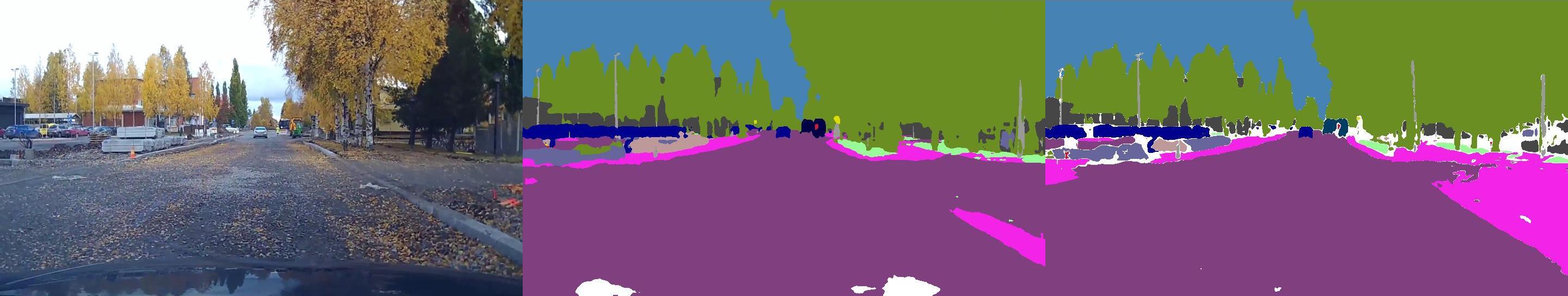
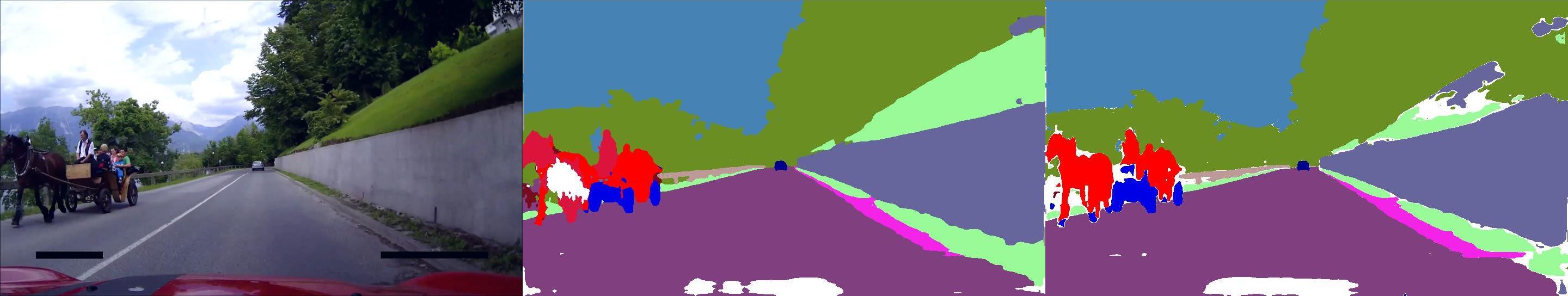
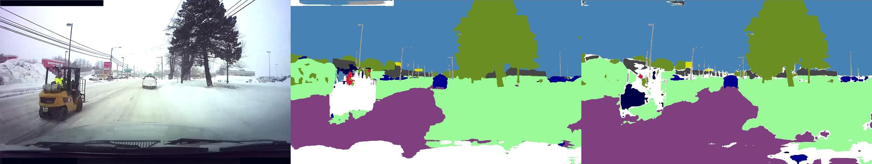
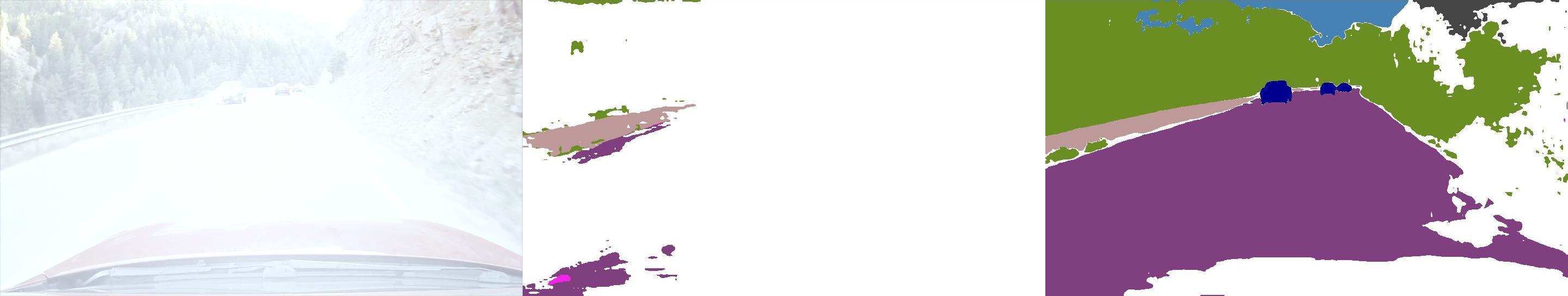
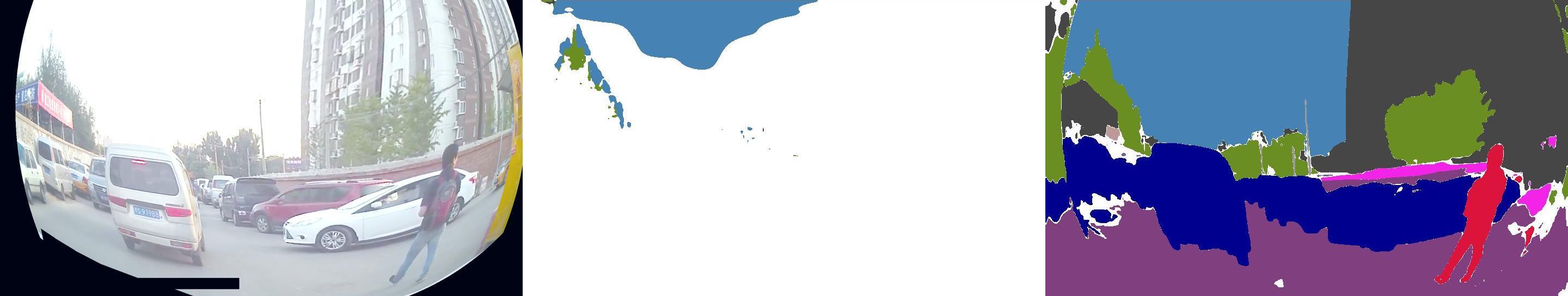
Figure 3: Qualitative performance of our two submissions to the WildDash benchmark. Each triplet contains a test image (left), the output of the two-head model (center), and the output of the model trained to predict uniform distribution in outliers (right). Rows represent inlier images (1), outlier objects in inlier context (2), inlier images with hazards (3), out-of-scope negatives (4), and abstract negatives (5). The two-head model produces more outlier detections while performing better in classic images (cf. Table 1).

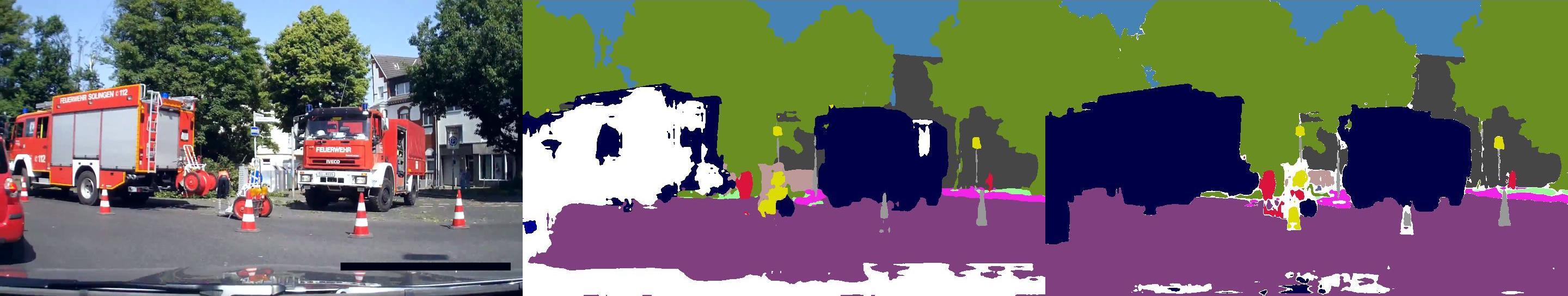
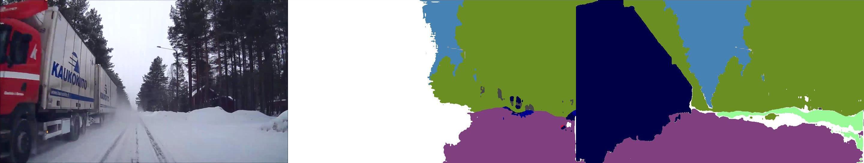
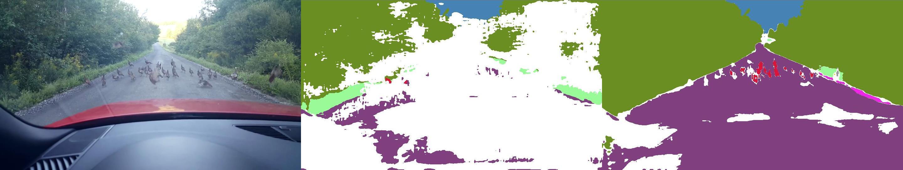
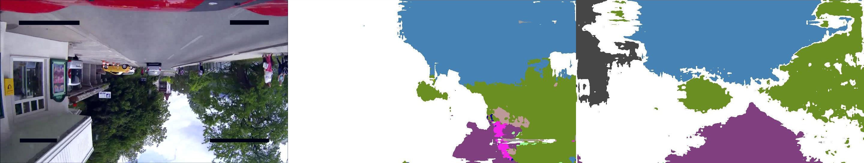
Figure 4: Failure cases on WD test arranged as in Fig. 3. Top: the two-head model predicts outliers at trucks. Bottom left: both models fail to accurately detect birds on the road. Bottom right: both models exchange road and sky due to position bias (late experiments show this can be improved with training on smaller crops and scale jittering).

4.6 Discussion

Validation on LSUN and WildDash val suggests that detecting entire outlier images is an easy problem. A useful practical application of this result would be a module to detect whether the camera is out of order due to being covered, dirty or faulty. Validation on pasted Pascal animals suggests that detecting outliers in inlier context is somewhat harder but still within reach of modern techniques.

Evaluation on WildDash test shows that our models outperform previous published approaches. We note significant improvement with respect to state of the art in classic and negative images, as well as in average mIoU score. Our models successfully detect all abstract and out-of-scope negatives [47], even though much of this content is not represented by ImageNet-1k classes.

Future work should address further development of open-set evaluation datasets such as [47, 3]. In particular, the community would benefit from substantially larger negative test sets which should include diverse non-ImageNet-1k content, as well as outlier objects in inlier context and inlier objects in outlier context.

5 Conclusion

We have presented an approach to combine semantic segmentation and dense outlier detection without significantly deteriorating either of the two tasks. We cast outlier detection as binary classification on top of a shared convolutional representation. This allows for solving both tasks with a single forward pass through a convolutional backbone. We train on inliers from standard road driving datasets (Vista, Cityscapes), and noisy outliers from a very diverse negative dataset (ImageNet-1k). The proposed training procedure tolerates inliers in negative training images and generalizes to images with mixed content (inlier background, outlier objects). We perform extensive open-set validation on WildDash val (inliers), LSUN val (outliers), and pasted Pascal objects (outliers). The results confirm suitability of the proposed training procedure. The proposed multi-head model outperforms the C-way multi-label model and the C+1-way multi-class model, while performing comparably to the C-way multi-class model trained to predict uniform distribution in outliers. We apply our two best models to WildDash test and set a new state of the art on the WildDash benchmark.

Appendix A Supplementary material

We use this supplement to further discuss the experiments from Section 4 of the main paper. We clarify the losses used for training the models and expand on the quantitative results described in the main paper by offering qualitative analysis of model outputs. Furthermore, we offer experiments with two additional outlier detection approaches applied to dense prediction: MC-dropout and trainable confidence.

In the first section we provide a detailed overview of the training losses. The results of the additional experiments can be seen at the beginning of the second section. The rest of the second and all of the third section are dedicated to illustrating validation experiments on WD-Pascal dataset. WD-Pascal is a set of images which we create by pasting instances of animals from PASCAL VOC 2007 dataset into WildDash validation images. We show that low AP scores on WD-Pascal are strongly affected by false positive detections in WildDash images which occur due to sensitivity to domain shift.

In the fourth section we give more examples of the performance of our submissions to the WildDash benchmark.

A.1 Review of loss functions

Segmentation can be viewed as multi-class classification. To train it, we use the negative log-likelihood loss for each pixel of the output. We use the softmax activation function on the output of the network. Additionally, as a class balancing techinque, the loss for each pixel can be weighted depending on the ground truth label. In our experiments we only used class balancing during the C+1 way multi-class training by setting the $\lambda_{\mathrm{C+1}}$ to 0.05 to account for the fact that outlier pixels outnumber inlier pixels for each individual class. In the case of the model with trainable confidence, the prediction is adjusted by interpolating between the original predictions and the target probability:

$$P^{\prime}(Y_{ij}=y_{ij}|\boldsymbol{x})=c_{ij}P(Y_{ij}=y_{ij}|\boldsymbol{x})+(1-c_{ij})y_{ij}$$ (1)

When considering segmentation as multi-label classification, we perform $C$ binary classifications. We do this by using sigmoid activation function instead of the softmax activation function at the output of the network. In this setup, each sample is simultaneously a positive for its own class and a negative for the rest of the classes. This setup also allows us to use outliers during training. The ouliers serve as negatives for all of the $C$ binary classifiers.

To improve the segmentation, we use auxiliary losses at 4, 8, 16 and 32 times lower resolutions. The expected output at each resolution is a distribution over all segmentation classes. We calculate this distribution across the corresponding window from the ground truth labels at full resolution. We only take into account pixels that have a valid label. Since we use soft targets at lower distributions, we use cross entropy loss between the expected distribution and the output of the network at a given resolution.

The model with trainable confidence is trained by using the confidence loss alongside the multi-class classifier loss. The confidence loss can be interpreted as the negative log-likelihood loss where the expected output is always 1, that is to say, the network is always expected to be confident. [11] show that the confidence tends to converge into unity and that confidence training tends to be a strong regularizer. To prevent the former they suggest adjusting $\lambda_{\mathrm{C}}$ so that $\mathcal{L}_{\mathrm{C}}$ tends toward a hyperparameter $\beta$ throughout training. To minimize the latter, they also suggest applying Equation 1 only on half of the batch at each iteration. We set $\beta$ to 0.15, and perform Equation 1 on every second batch.

The model with the separate outlier detection head is trained with the additional negative log-likelihood loss. This loss is calculated between the output of the second head and the ground truth labels indicating whether a pixel is an inlier or an outlier.

The C-way multi-class approach can be trained to emit uniform distribution at outlier samples. This is done by minimizing the Kullback-–Leibler (KL) divergence between the uniform distribution and the output of the network.

Tables 7 and 8 present an overview of losses used in our experiments. We use the following assumptions in our notation: $\boldsymbol{x}$ is an input image, $\boldsymbol{y}$ contains ground truth segmentation into $N_{\mathrm{C}}$ classes and $\boldsymbol{z}$ contains ground truth indicating whether a pixel is an inlier (label 1) or an outlier (label 0).

Some pixels can be ignored during training (e.g.the ego-vehicle). To indicate that these pixels should be ignored, they are given a label greater than the number of classes $N_{\mathrm{C}}$ in the ground truth segmentation image $\boldsymbol{y}$ and label $2$ in $\boldsymbol{z}$. When training with ouliers, $\boldsymbol{y}$ can be modified in two different ways: i) in the C+1-way multi-class setup, $N_{\mathrm{C}}$ is equal to C+1, the label of the outlier pixels is set to C+1, while the label of the ignored pixels needs to be greater than C+1; or ii) the label of the outlier pixel is set to any number greater $N_{\mathrm{C}}$.

Table 7: Losses used during training, with the following assumptions: $\boldsymbol{x}$ is an input image, $\boldsymbol{y}$ contains ground truth segmentation into $N_{\mathrm{C}}$ classes and $\boldsymbol{z}$ contains ground truth indicating whether a pixel is an inlier or an outlier. Dimensions of $\boldsymbol{x}$, $\boldsymbol{y}$ and $\boldsymbol{z}$ are $H\times W$.

Loss	Expression
multi-class classifier loss	$$\displaystyle\mathcal{L}_{\mathrm{MC}}=-{\sum}\limits_{i,j\in G_{x}}\lambda_{y_{ij}}[\![z_{ij}=1\wedge y_{ij}\leq N_{\mathrm{C}}]\!]\log P(Y_{ij}=y_{ij}|\boldsymbol{x}),$$ $$\displaystyle P(Y_{ij}=y_{ij}|\boldsymbol{x})=\frac{\exp s_{y_{ij}}^{ij}(\boldsymbol{x})}{\sum\limits_{c}\exp{s_{c}^{ij}(\boldsymbol{x})}}$$
multi-label classifier loss	$\displaystyle\mathcal{L}_{\mathrm{ML}}=-{\sum}\limits_{i,j\in G_{x}}{\sum}\limits_{c=1}^{N_{c}}[\![y_{ij}\leq N_{\mathrm{C}}]\!]\biggl{(}$ $\displaystyle[\![y_{ij}\neq c\vee z_{ij}=0]\!]\log\frac{1}{1+\exp s_{y_{ij}}^{ij}(\boldsymbol{x})}$ $\displaystyle+$ $\displaystyle[\![y_{ij}=c\wedge z_{ij}=1]\!]\log\frac{\exp s_{y_{ij}}^{ij}(\boldsymbol{x})}{1+\exp s_{y_{ij}}^{ij}(\boldsymbol{x})}\biggr{)}$
auxiliary loss	$$\displaystyle\mathcal{L}_{\mathrm{AUX}}=-{\sum}\limits_{r\in R}{\sum}\limits_{i,j\in G_{x}^{r}}[\![N_{ij}^{r}>\tfrac{r^{2}}{2}]\!]\mathbb{E}_{\boldsymbol{y}_{ij}^{r}}[\log P(Y_{ij}^{r}|\boldsymbol{x})],$$ $$\displaystyle y_{ijc}^{r}=\frac{1}{N_{ij}^{r}}{\sum}\limits_{l=ir}^{ir+r-1}{\sum}\limits_{k=jr}^{jr+r-1}[\![y_{kl}=c\wedge y_{kl}\leq N_{\mathrm{C}}]\!],$$ $$\displaystyle N_{ij}^{r}={\sum}\limits_{l=ir}^{ir+r-1}{\sum}\limits_{k=jr}^{jr+r-1}[\![y_{kl}\leq N_{\mathrm{C}}]\!]$$
separate outlier detection head loss	$\displaystyle\mathcal{L}_{\mathrm{TH}}=-{\sum}\limits_{i,j\in G_{x}}[\![z_{ij}\leq 1]\!]\log P(Z_{ij}=z_{ij}|\boldsymbol{x})$
Kullback Leibler divergence	$\displaystyle\mathcal{L}_{\mathrm{KL}}={\sum}\limits_{i,j\in G_{x}}[\![z_{ij}=0]\!]\mathrm{KL}(\mathcal{U}\parallel P(Y_{ij}|\boldsymbol{x}))$
confidence loss	$\displaystyle\mathcal{L}_{\mathrm{C}}=-{\sum}\limits_{i,j\in G_{x}}[\![y_{ij}\leq N_{\mathrm{C}}]\!]\log(c_{ij}|\boldsymbol{x})$

Table 8: Total training losses

Model	Total loss
C$\times$ multi-class, C+1$\times$ multi-class	$\lambda_{\mathrm{MC}}\mathcal{L}_{\mathrm{MC}}+\lambda_{\mathrm{AUX}}\mathcal{L}_{\mathrm{AUX}}$
C$\times$ multi-class with confidence head	$\lambda_{\mathrm{MC}}\mathcal{L}_{\mathrm{MC}}+\lambda_{\mathrm{C}}\mathcal{L}_{\mathrm{C}}+\lambda_{\mathrm{AUX}}\mathcal{L}_{\mathrm{AUX}}$
C$\times$ multi-label	$\lambda_{\mathrm{ML}}\mathcal{L}_{\mathrm{ML}}+\lambda_{\mathrm{AUX}}\mathcal{L}_{\mathrm{AUX}}$
C$\times$multi-class with outliers	$\lambda_{\mathrm{MC}}\mathcal{L}_{\mathrm{MC}}+\lambda_{\mathrm{KL}}\mathcal{L}_{\mathrm{KL}}+\lambda_{\mathrm{AUX}}\mathcal{L}_{\mathrm{AUX}}$
two heads	$\lambda_{\mathrm{MC}}\mathcal{L}_{\mathrm{MC}}+\lambda_{\mathrm{TH}}\mathcal{L}_{\mathrm{TH}}+\lambda_{\mathrm{AUX}}\mathcal{L}_{\mathrm{AUX}}$

A.2 Validation of Dense Oultier Detection Approaches

Table 9 is an extension of Table 2 from the main paper. It provides results of outlier detection and semantic segmentation for a model with a separate confidence head [11] and a semantic segmentation model trained using Monte Carlo (MC) dropout after each of the dense and upsampling layers, with epistemic uncertainty used as a criterion for outlier detection [24, 23]. The MC-dropout is also used during the inference phase, meaning that the final output of the model is the mean value of 50 forward passes. Both of the models trained with dropout perform outlier detection better than the baseline model. They, however, perform worse than any of the models trained with noisy negatives. Out of all of the tested models, the model with the confidence head provides the worst outlier detection accuracy. We observe a drop in semantic segmentation accuracy on WildDash validation dataset when compared to the baseline model for all of the additional models.

Table 9: Validation of dense outlier detection approaches. WD denotes WildDash val.

Model	ImageNet	AP WD-LSUN	AP WD-Pascal	mIoU WD
C$\times$ multi-class, dropout 0.2	✗	$64.09\pm 0.97$	11.87	49.13
C$\times$ multi-class, dropout 0.5	✗	$63.37\pm 1.13$	13.18	47.25
confidence head	✗	$54.40\pm 0.80$	4.41	45.38

Figure 5 gives a qualitative insight into the results from Table 2 of the main paper. It explores validation performance of different outlier detector variants described in Section 3.2 of the main paper.

Row 1 contains images from WD-Pascal. Each subsequent row shows the output of a different outlier detector. Row 2 corresponds to the C-way multi-class model trained without negative samples (baseline). This model assigns high outlier probabilty at semantic borders. Consequently it detects borders of outlier patches. It is however unable to detect entire outlier objects. Since the baseline model with ODIN, the model with the confidence head and the models trained with dropout perform qualitatively similarly, we omit those results for brevity.

Row 3 shows the output of the C+1-way multi-class model. This model had the lowest AP score. Qualitative analysis suggests that this model makes more false outlier predictions which in turn lowers the AP score.

Row 4 shows the C-way multi-label model and row 5 shows the C-way multi-class model. They perform similarly, though the C-way multi-label model seems to be more robust to domain shift (cf. column 4). These models are more successful at outlier detection than the baseline model, though they also assign a high outlier probability to border pixels.

Row 6 shows the output of the two-head model. It is successful at detecting outliers without falsely detecting borders as outliers. Furthermore, its detections tend to be coarser than in other models.

All models trained with ImageNet-1k-bb have a problem with large domain shift as exemplified in column 4. This indicates that it would be very hard to achieve high AP scores on WD-Pascal since images with large domain shift are perceived as equally foreign as the pasted Pascal objects. Column 3 shows that models trained using negative data classify the windshield wiper as outlier. This is interesting when compared to the model which has seen WildDash validation during training (row 3 of Figure 10). This is further discussed in Section 3.

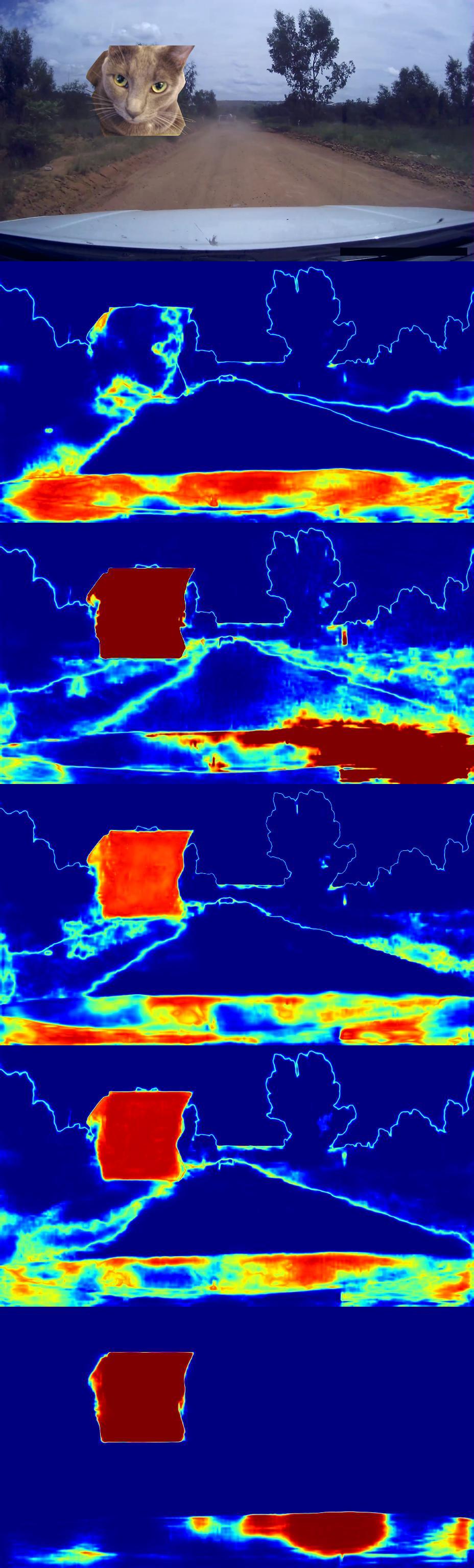
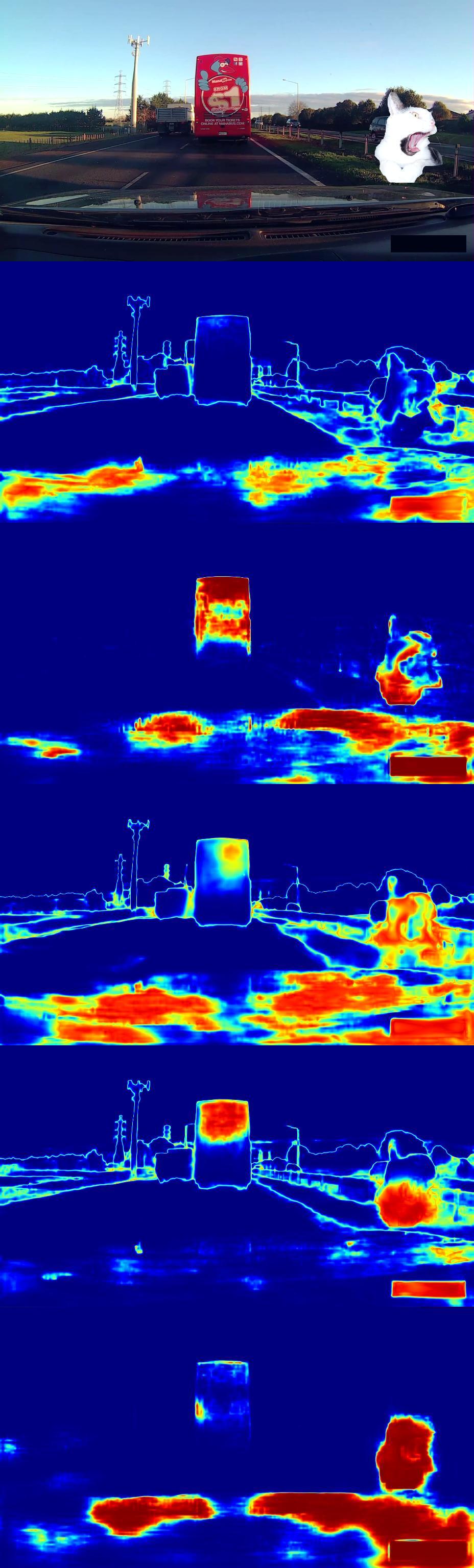
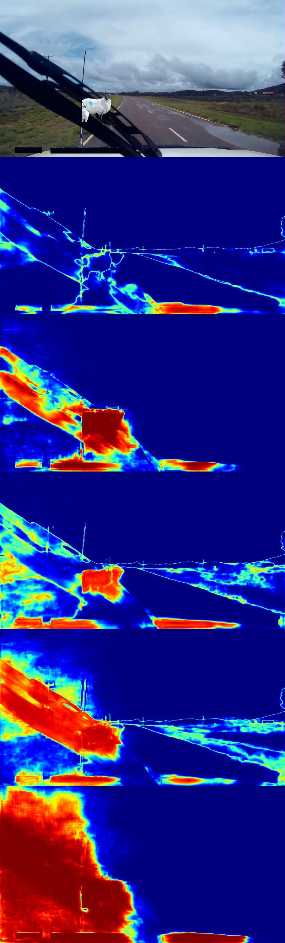
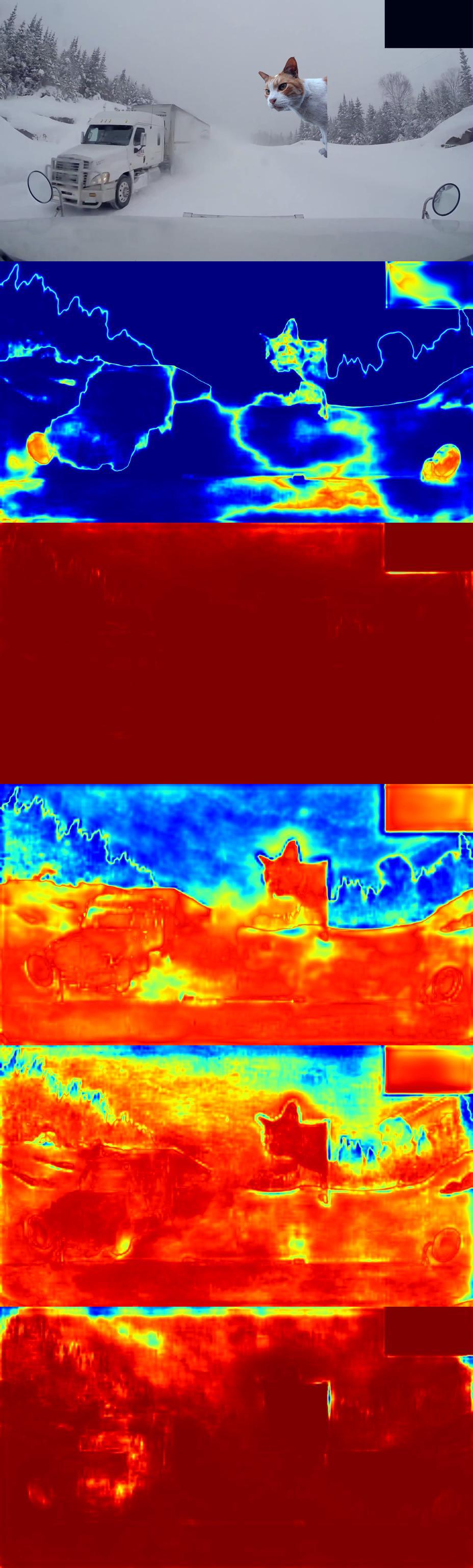
Figure 5: Dense outlier detection with models presented in Table 2. Row 1 shows Wilddash val images with pasted PASCAL VOC 2007 animals. Row 2 shows outlier probabilities obtained with the C-way multi-class model trained without negatives. Red colour indicates a high probability that a pixel is an outlier. Subsequent rows correspond to models trained with noisy negatives: the C+1-way multi-class model (row 3), the C-way multi-label model (row 4), the C-way multi-class model (row 5) and the two-head model (row 6).

A.3 Influence of the Training Data

Figure 6 illustrates the validation performance of the two-head model depending on the inlier training dataset, which was shown in Table 4 of the paper. Column 1 shows four validation images.

Column 2 presents the corresponding results of the two-head model trained on Cityscapes. This model classifies all of the WildDash pixels as outliers. This indicates that models trained on Cityscapes are very sensitive to domain shift.

Column 3 shows that the two-head model trained on Vistas dataset is significantly better at outlier detection. This improvement indicates that models trained on Vistas show more resilience to domain shift.

Column 4 depicts a model trained on both Vistas and Cityscapes. It performs similarly to the model trained on Vistas.

Interestingly, the model trained on Vistas shows more resilience to unusual conditions (dark image in row 4, unusual vehicle in row 3), while the model trained on combined datasets shows more precision in normal situations (grass in row 1, road in row 2).

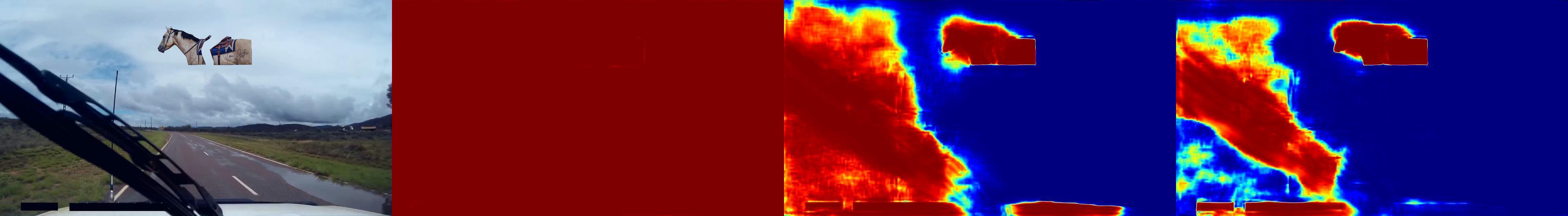
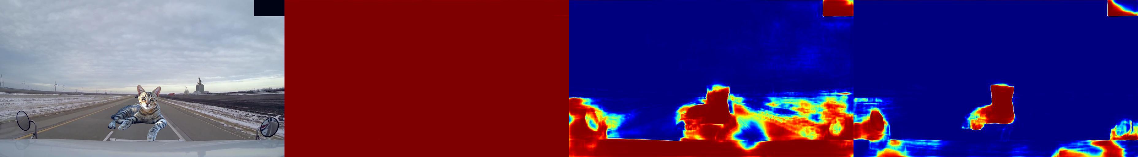
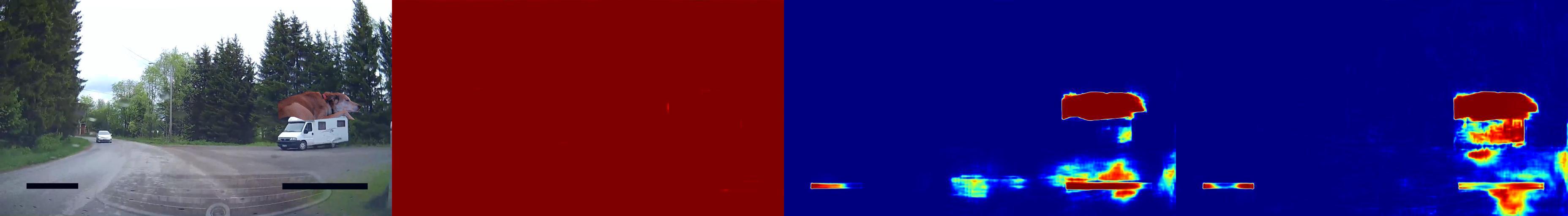
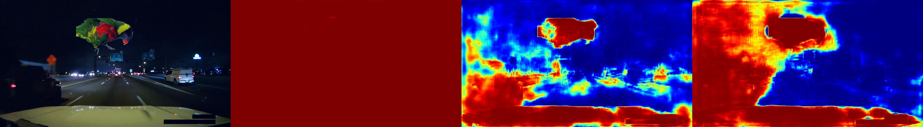
Figure 6: Outlier detection with two-head models trained on different inlier datasets. All models have been trained with pasted noisy negatives from ImageNet-1k-bb as presented in from Table 4. Column 1 contains Wilddash images with pasted PASCAL VOC 2007 animals. Columns 2-4 show predictions of models trained on Cityscapes, Vistas, and Cityscapes and Vistas, respectively. Red colour indicates a high probability that a pixel is an outlier.

Figure 7 shows the results of the two-head model depending on the negative training dataset (cf. Table 5).

The first column shows the validation images.

The second column shows the model trained using ImageNet-1k-full without pasting. It tends to make coarse predictions. Consequently it is unable to detect small outlier patches.

The third column illustrates the model trained using ImageNet-1k-full with pasting. It is better at detecting outlier samples. It is however sensitive to domain shift. This is because of the increased overlap between positive and negative images (in classes such as sky, vegetation or road which appear often in the backgrounds of ImageNet images).

The last column shows the model trained using ImageNet-1k-bb with pasting which performs the best both qualitatively and quantitatively.

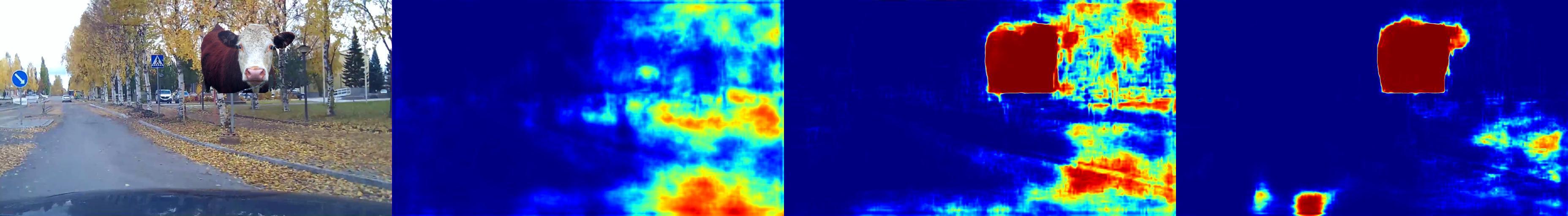
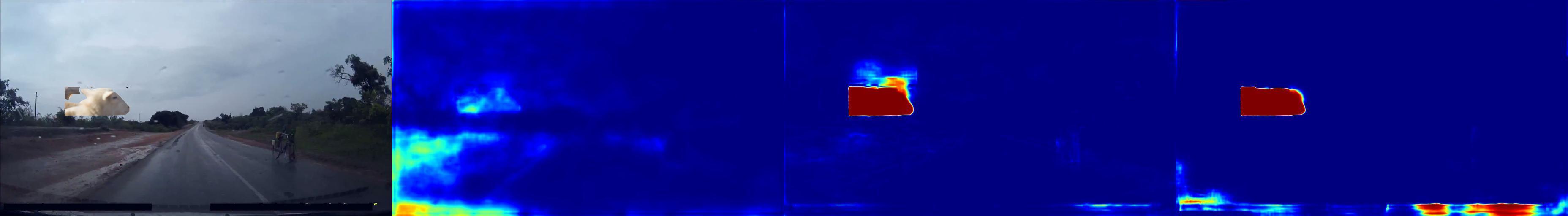
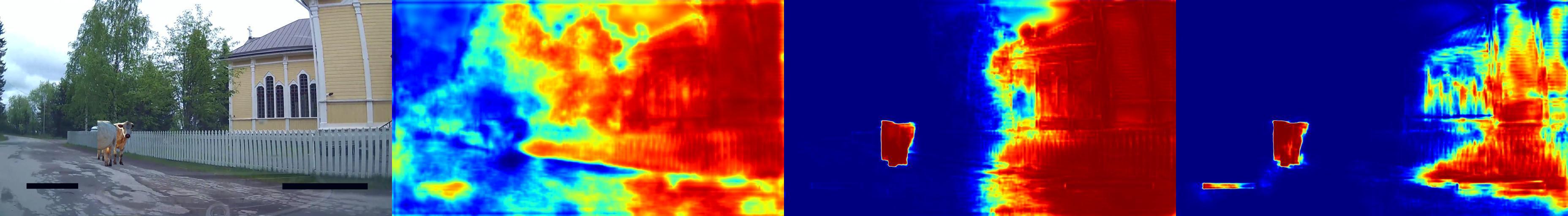
Figure 7: Outlier detection with two-head models trained on different negative datasets. All models have been trained by pasting negatives into inliers from Vistas as presented in Table 5. Column 1 shows original Wilddash images with pasted PASCAL VOC 2007 animals. Columns 2-4 show predictions of models trained with noisy negatives from Imagnet-1k-full (without pasting), ImageNet-1k-full (with pasting), and ImageNet-1k-bb (with pasting), respectively. Red colour indicates a high probability that a pixel is an outlier.

A.4 Comparing the Two-Head and C-way Multi-class Models

Figure 8 accompanies Table 1 of the main paper. It presents the combined output of the two-head model (column 2) and the C-way model trained with ImageNet-1k images (column 3) on images from WildDash test set (column 1).

The first four rows show images taken in normal conditions, while the last two rows show oulier images.

The C-way model tends to classify small objects (cf. poles in image in row 3) as well as distant objects (cf. trucks in the distance in the image in the third row) as outliers. This model makes more false outlier detections in typical traffic scenes.

Furthermore, the two-head model performs better in negative images. Output of the C-way model on negative images contains small patches not classified as outliers.

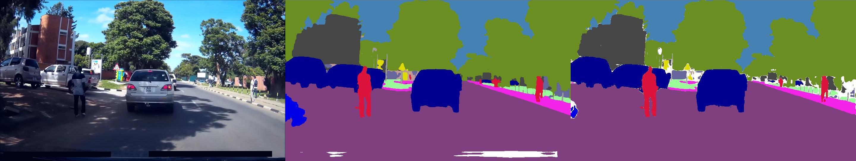
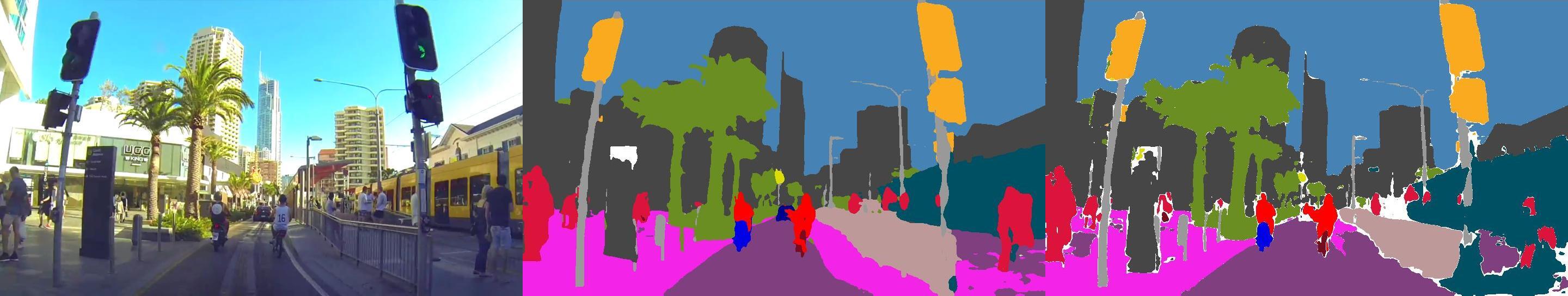
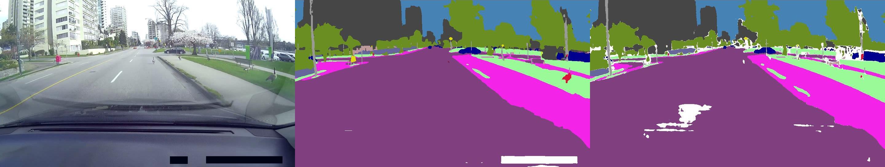
Figure 8: Qualitative performance on the WildDash benchmark. Each triplet contains a test image (left), the output of the two-head model (center), and the output of the C-way multi-class model trained to predict uniform distribution in outliers (right). The two-head model does not produce false positives at semantic borders (rows 1-4). Both models correctly recognize outliers in negative images (rows 5-6).

Figure 9 further clarifies Table 6 from the main paper. It illustrates impact of WildDash hazards on the output of the submitted models.

The results show that the two-head model is more sensitive to overexposure and distortion hazards, though it succeeds when the hazard is not severe (rows 1-4).

Row 5 contains an example of occlusion. Both of the models are able to successfully segment the torso or the person behind the pole but they struggle with the lower part. Row 6 contains an example of the particles hazard (rain on the windshiled), while row 7 contains an example of the variation hazard (with tank truck being an atypical example of a truck).

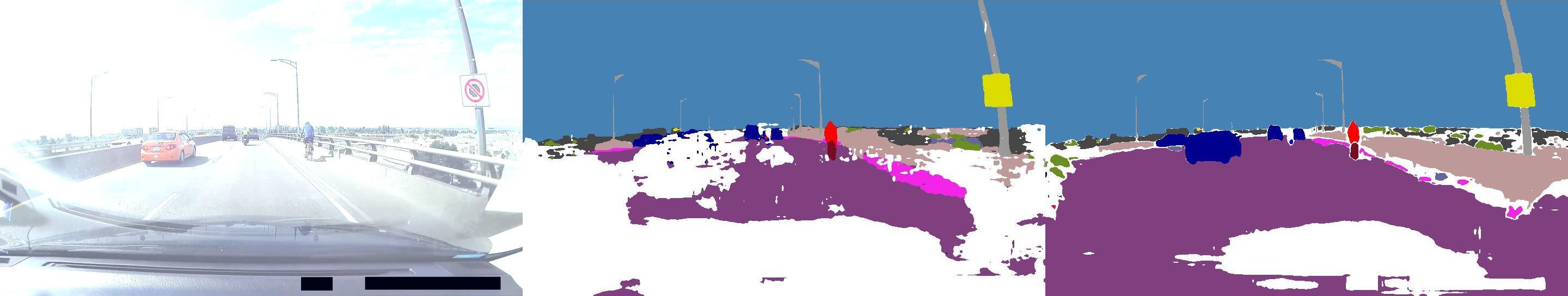
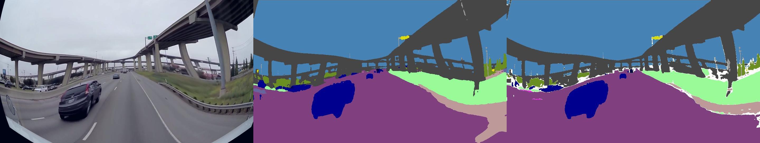
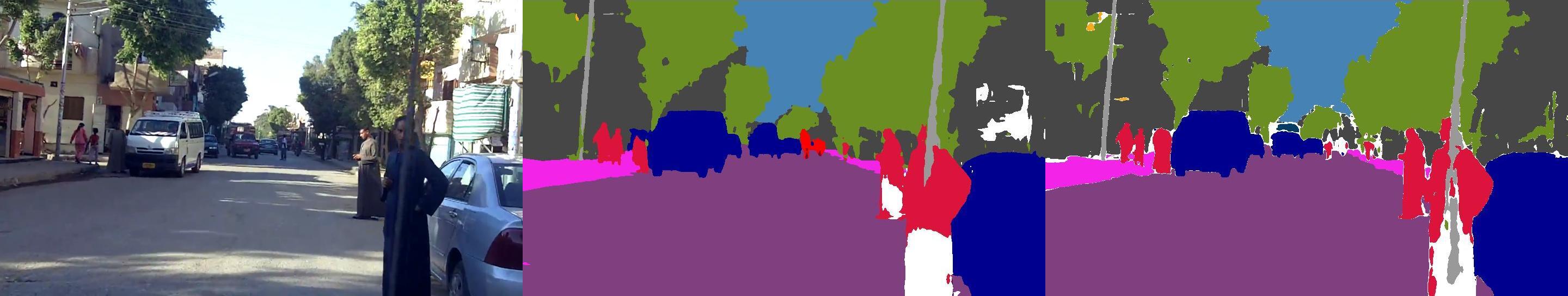
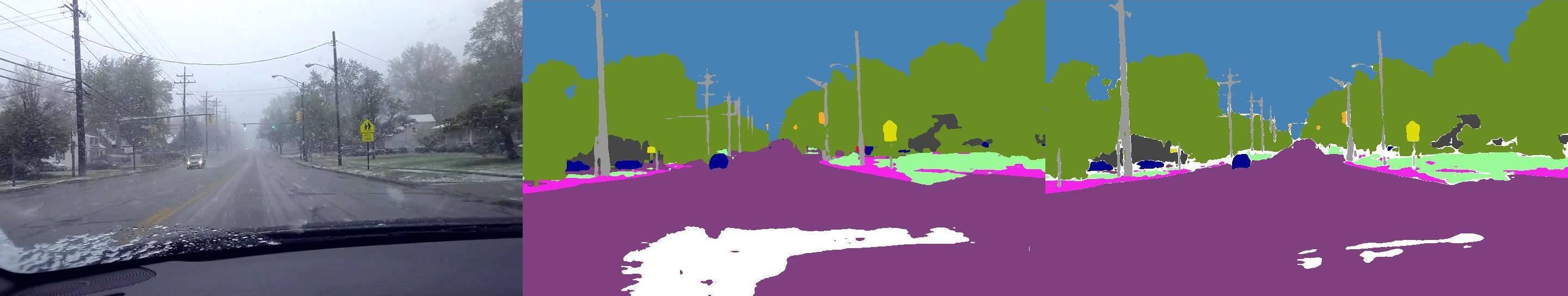
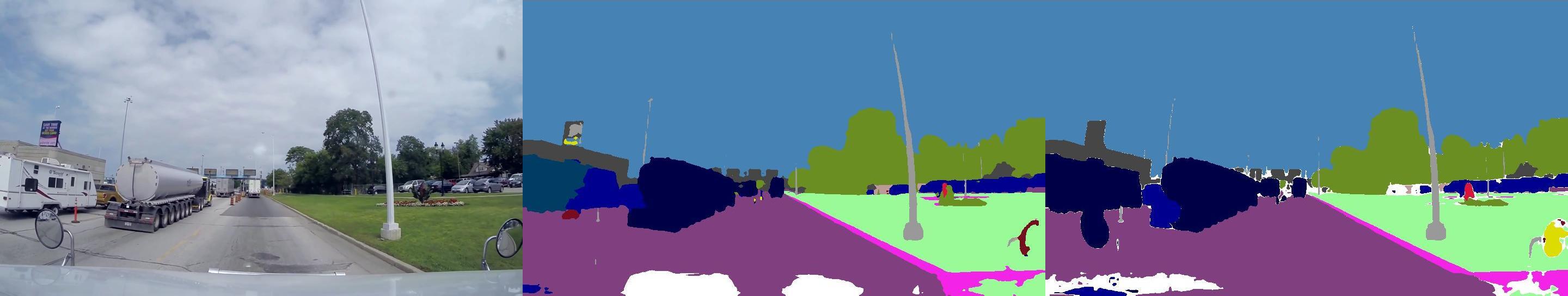
Figure 9: Qualitative performance on WildDash test images with overexposure and distortion hazards. Each triplet contains a test image (left), the output of the two-head model (center), and the output of the C-way multi-class model trained to predict uniform distribution in outliers (right). The two-head model rejects images with severe hazards.

Figure 10 expands on the failure cases shown in Figure 4 of the main paper which are worth exploring in future work.

The first two rows show images with animals on roads. Animals are usually classified as pedestrians. The two-head model classifies most of the pixels of the image in row 1 as outliers. Both of the models fail to classify the animals as outliers accurately.

The windshield wiper in the row 3 is classified as an inlier. This is because the submitted models were trained on Wilddash val which contains examples of images with windshields wipers. Those pixels are ignored during training but they still influence the features extracted by the dense feature extractor. This view is supported by Figure 5 where images in column 3 demonstrate that a model trained only on Vistas classifies windshield wipers as outliers. Handling ignored training pixels is a suitable direction for future work.

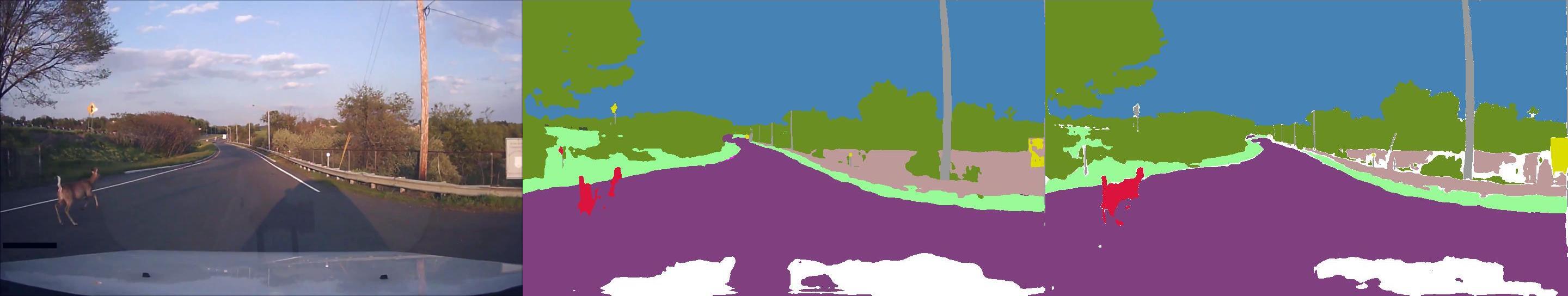
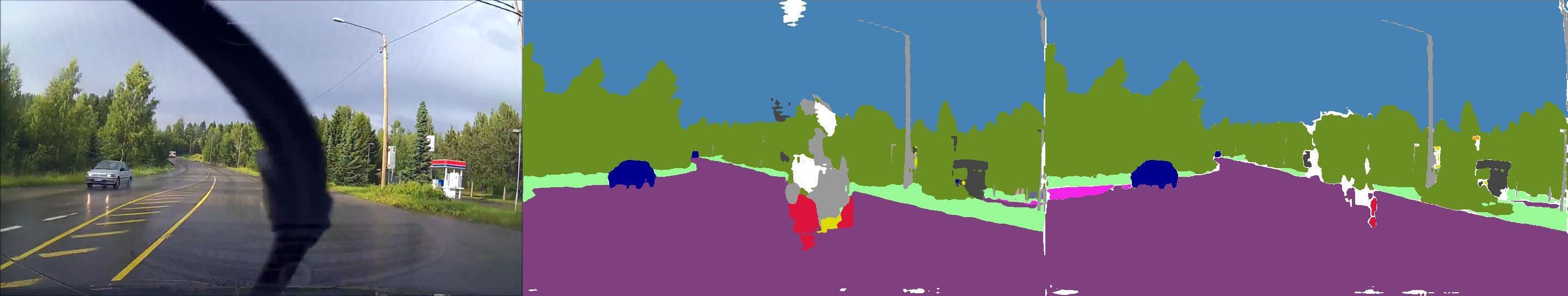
Figure 10: Qualitative performance of our two submissions to the WildDash benchmark. Each triplet contains a test image (left), the output of the two-head model (center), and the output of the model trained to predict uniform distribution in outliers (right). Rows 1-2 show that our current models are unable to correctly detect small outlier objects. Row 3 shows that the windshield wiper is recognized as inlier, which occurs due to its presence in WildDash val (cf. Figure 5).

References

- [1] Bengio, Y., Courville, A.C., Vincent, P.: Representation learning: A review and new perspectives. IEEE Trans. Pattern Anal. Mach. Intell. 35(8), 1798–1828 (2013)
- [2] Bevandic, P., Kreso, I., Orsic, M., Segvic, S.: Discriminative out-of-distribution detection for semantic segmentation. CoRR abs/1808.07703 (2018)
- [3] Blum, H., Sarlin, P., Nieto, J.I., Siegwart, R., Cadena, C.: The Fishyscapes benchmark: Measuring blind spots in semantic segmentation. CoRR abs/1904.03215
- [4] Brock, A., Donahue, J., Simonyan, K.: Large scale GAN training for high fidelity natural image synthesis. In: ICLR (2019)
- [5] Brostow, G.J., Shotton, J., Fauqueur, J., Cipolla, R.: Segmentation and recognition using structure from motion point clouds. In: ECCV. pp. 44–57 (2008)
- [6] Bulò, S.R., Porzi, L., Kontschieder, P.: In-place activated batchnorm for memory-optimized training of dnns. CoRR, abs/1712.02616, December 5 (2017)
- [7] Caruana, R.: Multitask learning. Machine Learning 28(1), 41–75 (Jul 1997). https://doi.org/10.1023/A:1007379606734
- [8] Chen, L.C., Zhu, Y., Papandreou, G., Schroff, F., Adam, H.: Encoder-decoder with atrous separable convolution for semantic image segmentation. In: ECCV (2018)
- [9] Cordts, M., Omran, M., Ramos, S., Scharwächter, T., Enzweiler, M., Benenson, R., Franke, U., Roth, S., Schiele, B.: The cityscapes dataset. In: CVPRW (2015)
- [10] Deng, J., Dong, W., Socher, R., Li, L., Li, K., Li, F.: Imagenet: A large-scale hierarchical image database. In: CVPR. pp. 248–255 (2009)
- [11] DeVries, T., Taylor, G.W.: Learning confidence for out-of-distribution detection in neural networks. CoRR abs/1802.04865 (2018)
- [12] Eigen, D., Fergus, R.: Predicting depth, surface normals and semantic labels with a common multi-scale convolutional architecture. ICCV pp. 2650–2658 (2015)
- [13] Everingham, M., Gool, L., Williams, C.K., Winn, J., Zisserman, A.: The pascal visual object classes (voc) challenge. Int. J. Comput. Vision (2010)
- [14] Geiger, A., Lenz, P., Stiller, C., Urtasun, R.: Vision meets robotics: The kitti dataset. International Journal of Robotics Research (IJRR) (2013)
- [15] Goodfellow, I.J., Pouget-Abadie, J., Mirza, M., Xu, B., Warde-Farley, D., Ozair, S., Courville, A.C., Bengio, Y.: Generative adversarial nets. In: NIPS (2014)
- [16] Guo, C., Pleiss, G., Sun, Y., Weinberger, K.Q.: On calibration of modern neural networks. In: ICML. pp. 1321–1330 (2017)
- [17] He, K., Gkioxari, G., Dollár, P., Girshick, R.: Mask R-CNN. In: ICCV (2017)
- [18] He, K., Zhang, X., Ren, S., Sun, J.: Spatial pyramid pooling in deep convolutional networks for visual recognition. In: ECCV. pp. 346–361 (2014)
- [19] He, K., Zhang, X., Ren, S., Sun, J.: Deep residual learning for image recognition. CVPR pp. 770–778 (2016)
- [20] Hendrycks, D., Gimpel, K.: A baseline for detecting misclassified and out-of-distribution examples in neural networks. In: ICLR (2017)
- [21] Hendrycks, D., Mazeika, M., Dietterich, T.: Deep anomaly detection with outlier exposure. In: ICLR (2019)
- [22] Huang, G., Liu, Z., Weinberger, K.Q.: Densely connected convolutional networks. In: CVPR (2017)
- [23] Kendall, A., Badrinarayanan, V., Cipolla, R.: Bayesian segnet: Model uncertainty in deep convolutional encoder-decoder architectures for scene understanding. CoRR abs/1511.02680 (2015)
- [24] Kendall, A., Gal, Y.: What uncertainties do we need in bayesian deep learning for computer vision? In: NIPS. pp. 5574–5584 (2017)
- [25] Kong, S., Fowlkes, C.: Pixel-wise attentional gating for parsimonious pixel labeling. In: arxiv 1805.01556 (2018)
- [26] Kreso, I., Krapac, J., Segvic, S.: Ladder-style densenets for semantic segmentation of large natural images. In: ICCV CVRSUAD 2017. pp. 238–245 (2017)
- [27] Kreso, I., Krapac, J., Segvic, S.: Efficient ladder-style densenets for semantic segmentation of large images. CoRR abs/1905.05661 (2019)
- [28] Kreso, I., Orsic, M., Bevandic, P., Segvic, S.: Robust semantic segmentation with ladder-densenet models. CoRR abs/1806.03465 (2018)
- [29] Lakshminarayanan, B., Pritzel, A., Blundell, C.: Simple and scalable predictive uncertainty estimation using deep ensembles. In: NIPS. pp. 6402–6413 (2017)
- [30] Lee, K., Lee, H., Lee, K., Shin, J.: Training confidence-calibrated classifiers for detecting out-of-distribution samples. In: ICLR (2018)
- [31] Lee, K., Lee, K., Lee, H., Shin, J.: A simple unified framework for detecting out-of-distribution samples and adversarial attacks. In: NeurIPS (2018)
- [32] Liang, S., Li, Y., Srikant, R.: Enhancing the reliability of out-of-distribution image detection in neural networks. In: ICLR (2018)
- [33] Lin, T., Dollár, P., Girshick, R.B., He, K., Hariharan, B., Belongie, S.J.: Feature pyramid networks for object detection. In: CVPR. pp. 936–944 (2017)
- [34] Meletis, P., Dubbelman, G.: Training of convolutional networks on multiple heterogeneous datasets for street scene semantic segmentation. In: IV (2018)
- [35] Nalisnick, E.T., Matsukawa, A., Teh, Y.W., Görür, D., Lakshminarayanan, B.: Do deep generative models know what they don’t know? In: ICLR (2019)
- [36] Neuhold, G., Ollmann, T., Bulò, S.R., Kontschieder, P.: The mapillary vistas dataset for semantic understanding of street scenes. In: ICCV (2017)
- [37] Ngiam, J., Khosla, A., Kim, M., Nam, J., Lee, H., Y. Ng, A.: Multimodal deep learning. In: ICML. pp. 689–696 (2011)
- [38] Sabokrou, M., Khalooei, M., Fathy, M., Adeli, E.: Adversarially learned one-class classifier for novelty detection. In: CVPR. pp. 3379–3388 (2018)
- [39] Scheirer, W.J., de Rezende Rocha, A., Sapkota, A., Boult, T.E.: Toward open set recognition. IEEE Trans. Pattern Anal. Mach. Intell. 35(7), 1757–1772 (2013)
- [40] Shafaei, A., Schmidt, M., Little, J.J.: Does your model know the digit 6 is not a cat? A less biased evaluation of ”outlier” detectors (2018)
- [41] Smith, L., Gal, Y.: Understanding measures of uncertainty for adversarial example detection. In: UAI. vol. abs/1803.08533 (2018)
- [42] Torralba, A., Efros, A.A.: Unbiased look at dataset bias. In: CVPR (June 2011). https://doi.org/10.1109/CVPR.2011.5995347
- [43] Vyas, A., Jammalamadaka, N., Zhu, X., Das, D., Kaul, B., Willke, T.L.: Out-of-distribution detection using an ensemble of self supervised leave-out classifiers. In: ECCV (2018)
- [44] Yu, F., Koltun, V., Funkhouser, T.: Dilated residual networks. In: CVPR (2017)
- [45] Yu, F., Zhang, Y., Song, S., Seff, A., Xiao, J.: LSUN: construction of a large-scale image dataset using deep learning with humans in the loop (2015)
- [46] Zamir, A.R., Sax, A., Shen, W.B., Guibas, L.J., Malik, J., Savarese, S.: Taskonomy: Disentangling task transfer learning. In: CVPR (2018)
- [47] Zendel, O., Honauer, K., Murschitz, M., Steininger, D., Fernandez Dominguez, G.: Wilddash - creating hazard-aware benchmarks. In: ECCV (September 2018)
- [48] Zendel, O., Murschitz, M., Humenberger, M., Herzner, W.: How good is my test data? introducing safety analysis for computer vision. International Journal of Computer Vision 125(1-3), 95–109 (2017)
- [49] Zhao, H., Shi, J., Qi, X., Wang, X., Jia, J.: Pyramid scene parsing network. In: CVPR (2017)