Adaloss: Adaptive Loss Function for Landmark Localization

Abstract

Landmark localization is a challenging problem in computer vision with a multitude of applications. Recent deep-learning based methods have shown improved results by regressing likelihood maps (i.e. heatmaps) instead of regressing the coordinates directly. However, setting the precision of these regression targets during the training has been a cumbersome process since it creates a trade-off between trainability vs. localization accuracy. Using precise targets introduces a significant sampling bias and hence makes the training more difficult, whereas using imprecise targets results in inaccurate landmark detectors. In this paper, we introduce “Adaloss”, an objective function that adapts itself during the training by updating the target precision based on the training statistics. This approach does not require setting problem-specific parameters and shows improved stability in training and better localization accuracy in inference. We demonstrate the effectiveness of our proposed method in three very different applications of landmark localization: 1) the challenging task of precisely detecting catheter tips in medical X-ray images, 2) localizing surgical instruments in endoscopic images, and 3) localizing facial features on in-the-wild images where we show state-of-the-art results on the 300-W benchmark dataset.

1 Introduction

Landmark localization is a fundamental problem in computer vision with far-reaching impact on a myriad of applications in multiple domains. Whether the goal is to analyze the attentiveness of a driver [1], interpret sign language [2], plan aortic valve surgeries [3], estimate body pose for human-computer interaction [4], or detect surgical instruments in endoscopic procedures [5], the first step usually involves precise detection of relevant semantic keypoints in the given input images.

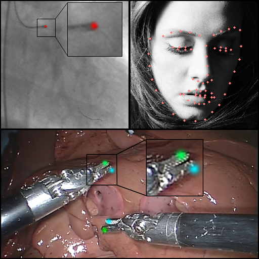
Figure 1: From one task to another, landmark localization has far reaching impact on multiple domains. (top-left) Detection of the tip of a catheter in a medical X-ray image, where the tolerance for practical usefulness is about 1 pixel at 256 x 256 resolution and annotations are very precise. (top-right) Facial feature localization, where some landmarks can be defined very precisely (e.g. eye corners), but others cannot be defined as precisely (e.g. chin landmarks). (bottom) Surgical instrument detection in endoscopic procedures, where the inherent occlusions and the viewpoint make it a challenging task.

Similar to the other fundamental computer vision problems such as object classification and segmentation, landmark localization has also seen a tremendous progress in recent years due to the availability of large datasets (e.g. [6, 5, 7, 8, 9]), improvements in training deep neural networks (e.g. [10, 11, 12, 13]), and availability of more computational resources.

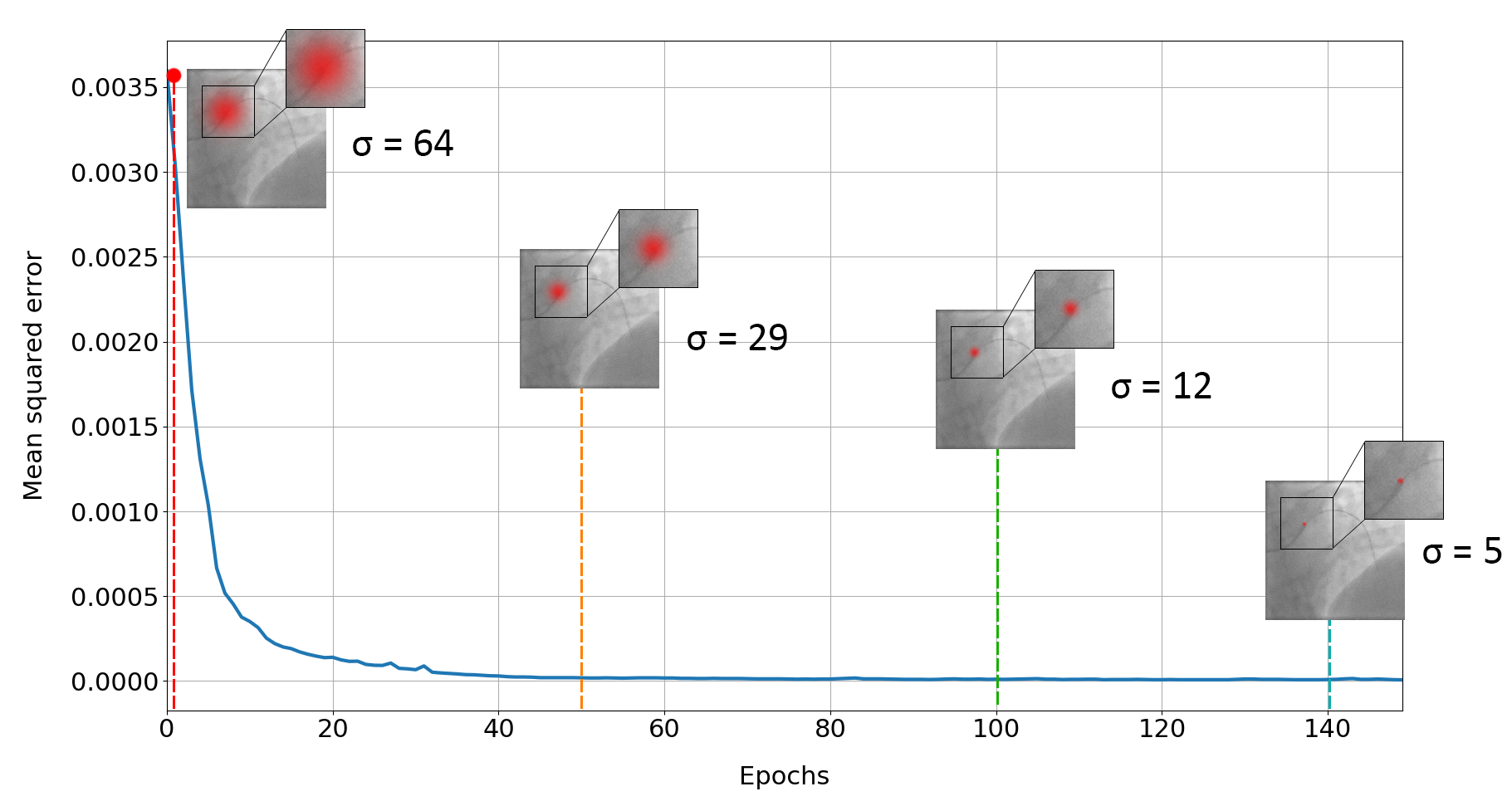
Figure 2: Evolution of Adaloss during training. In the early stages, Adaloss uses a large variance for the the target heatmaps. As the training progresses, Adaloss gradually decreases the target variance until reaching the optimal value for the given application.

Most existing deep-learning based methods formulate the landmark localization problem as a structured output regression problem where the landmark locations are either represented as a set of image coordinates [14, 15], or as a set of likelihood maps (i.e. heatmaps) [16, 17, 18, 19, 20]. While the former representation certainly provides a compact output, it has several undesirable properties such as: 1) forcing the network to learn the arbitrary mapping between the appearance of a landmark and its image coordinates, 2) outputting a single target location for each landmark instead of a number of candidate locations, and 3) forcing the design of explicit mechanisms for handling missing landmarks. As a result, these networks are usually harder to train and their output is less usable as a pre-processing step of more complex vision tasks. On the other hand, training deep networks to regress likelihood maps as landmark locations does not suffer from these limitations.

A ubiquitous way of defining these target likelihood maps in training is creating multi-variate Gaussian distributions centered at the target landmark locations [16, 17, 18, 19, 20, 21, 22, 23, 24]. The main concern here is appropriately setting the variance of these Gaussian distributions. Ideally, one would use the smallest possible variance (practically a delta function) while generating these target heatmaps so that the resulting detectors will be as precise and as accurate as possible. However, this does not work in practice. First, there is an inherited uncertainty and inconsistency in the human annotations [25] that needs to be considered during the training. Furthermore, training deep networks with highly sparse output distributions is difficult. This may be attributed to the significant sample bias in the outputs. With such bias during training, the networks quickly degenerate to all empty outputs and then over the course of the training they attempt to recover peaks around the target locations of various samples. Existing methods try to address these problems by application-dependent and add-hoc solutions, such as using very low learning rates [17, 26], arbitrarily weighting the target heatmaps [27, 28], or inevitably sacrificing the inference accuracy by using Gaussian distributions with larger variances.

In this paper, we introduce a novel, application-independent method for landmark localization, which addresses the aforementioned limitations. Our approach, which we refer to as “Adaloss”, indirectly adapts the objective function throughout the training by updating the training targets (see Figure 2). Adaloss begins the training by using targets with large variances, and then iteratively adjusts the target variances based on landmark-specific training statistics. Effectively, Adaloss provides an implicit “curriculum” for training.

Besides being easy to develop and integrate into existing training pipelines, Adaloss also increases the robustness of the training in applications with highly sparse target distributions, is less sensitive to initial learning rate, and requires fewer iterations to converge. It also generates more stable networks [29] and is capable of producing highly accurate landmark detectors in multiple domains. We demonstrate the effectiveness of our method in three very different applications of landmark localization: 1) detecting catheter tips in X-ray images where a single instance of a single landmark needs to be localized very precisely, 2) facial feature localization where single instances of multiple landmarks need to be localized in varying precision, where we show state-of-the-art results, and 3) detecting surgical instruments in endoscopy images where multiple instances of multiple landmarks need to be localized very precisely.

2 Related work

Availability of large-scale datasets [9, 8] and powerful GPUs allowed deep neural network based methods to outperform former methods on landmarks detection. Toshev et al. were the first to reach state of the art results with a DNN on the FLIC dataset [9] with DeepPose [30]. Their approach directly regress the coordinates of the body joints. Later on, Thompson et al. [16] proposed to focus on regressing heatmaps centered in the body joint locations instead of directly predicting the coordinates. This method outperformed direct coordinate regression method especially on challenging images. The intuition here was that directly regressing coordinates adds unnecessary learning complexity by trying to map RGB to XY coordinates. They also proposed to mix deep convolutional networks with graphical models by jointly training a Markov Random Field to model the correlation between the body keypoints.

Wei et al. [21] proposed to use deeper convolutional networks for directly regressing the heatmaps, by using multiple encoding-decoding networks iteratively, with intermediate supervision. This method was then improved by Newell et al. [17] who extended the networks by adding skip-connections between the convolution and deconvolution modules to better combine the features across multiple scales. Their proposed stacked hourglass architecture is as of today one of the most common architectures for landmark localization networks. Dong et al. [31] recently proposed a new method for improving temporal consistency for detecting facial landmarks in videos by augmenting the training loss with a registration loss based on optical flows. Honari et al. [18] investigated the situation where precise annotations are only provided for a small subset. They proposed a multitasking framework which can leverage from imprecise annotations such as regression and classification annotation to improve precise annotation such as landmarks. Finally, Dong et al. [19] focused on augmenting the training data by introducing a new Generative Adversarial Network (GAN) [32] to generate a pool of style-aggregated face images, and showed state-of-the-art results on the challenging 300-W face dataset.

While most recent works focused on improving model architectures and data augmentation, our approach aims to propose a better objective function that may be used in any heatmap regression setup and does not require problem dependent parameters.

3 Adaloss

Adaloss, like many other deep-learning based landmark localization methods in the literature, represents the landmark locations as heatmaps. These heatmaps are created by placing multi-variate Gaussian distributions at the ground truth landmark locations. However, unlike existing methods, Adaloss does not use fixed target heatmaps throughout the training but instead updates them as the training progresses.

Adaloss begins the training with less precise (i.e. large variance) targets and iteratively makes them more precise (i.e. decrease the variance) during the training. This may be interpreted as progressively altering the difficulty of the task on hand and hence can be considered as a curriculum method. In the beginning, the network tries to solve an easier problem, and once that easy problem is solved, it moves on to another more difficult problem, but uses what is learned so far as a strong initialization.

However, to facilitate convergence during training, the curriculum must be appropriately defined. Here, we propose to use a simple additive update equation to set the variance for the target of each landmark, $l$ after each epoch, $t$ (note that, for keeping the notation simple, we are using “standard deviation” and $\sigma$, instead of “variance” and $\Sigma$ in our explanations, but depending on the application the target distributions may be one, two, or three dimensional):

$$\sigma^{l}_{t+1}=\sigma^{l}_{t}+\Delta\sigma^{l}_{t}$$ (1)

where, $\Delta\sigma^{l}_{t}$ is the change in the standard deviation for the target of landmark $l$ in epoch $t$. Note that for multi-variate tasks, we simply employ isotropic targets, where each diagonal element of the target variance is defined as in Equation 1.

A naive approach would be to set $\Delta\sigma^{l}_{t}=-k$ as a constant decay parameter, linearly decreasing the standard deviation after each epoch. Even though this naive approach may work for some problems it would not generalize well to all problems. For some, the constant decay would be very fast and hence would affect the trainability and for others, it would be very slow making the learning very inefficient. This is also the case when training for regressing multiple landmarks at once. Each of these individual landmark regression problems may have a varying level of difficulty and hence a constant decay parameter would not work for all.

Thus $\Delta\sigma^{l}_{t}$ should instead be set according to what has been observed in the training so far. Motivated by how AdaDelta [33] method sets the learning rate, we compute $\Delta\sigma^{l}_{t}$ based on the previous losses in a fixed window of size $w$. Note that, unlike AdaDelta, we use the actual loss values within this training window, and hence store the complete loss history instead of a running average. The history of the losses is defined as:

$$H^{l}_{t}=[L^{l}_{t-i}],0\leq i<w$$ (2)

To characterize the evolution of the loss function, we compute the loss variance $V^{l}_{t}$ which is set to be the variance of the values in the loss history vector $H^{l}_{t}$:

$$V^{l}_{t}=\frac{1}{w}\left(\sum_{i=0}^{w-1}(L_{t-i}^{l}-\mathop{{}\mathbb{E}}[H^{l}_{t}])^{2}\right)$$ (3)

If the loss variance is decreasing, it means that the loss function has not changed significantly during the last $w$ epochs. This suggests that the current landmark localization task (with the current standard deviation values) has converged or is close to convergence. In this case, it would help to decrease the standard deviation and attempt to solve a more difficult task. To this end, we compute the ratio of the previous variance $V^{l}_{t-1}$ with the current variance $V^{l}_{t}$ and use it as our standard deviation decay:

$$\Delta\sigma^{l}_{t}=1-\frac{V^{l}_{t-1}}{V^{l}_{t}}$$ (4)

For numerical stability, we also introduce a regularizer $\rho$ and finally, putting it all together, we obtain the following update equation for the target standard deviations:

$$\sigma^{l}_{t+1}=\sigma^{l}_{t}+\rho\cdot\left(1-\frac{V^{l}_{t-1}}{V^{l}_{t}}\right)$$ (5)

where we set $\sigma^{l}_{0}$ to be the quarter of the target resolution. This provides a good starting point as it addresses the sample bias problem associated with standard heaptmap regression methods.

Note that in Equation 5 an increase in the loss variance would cause a corresponding increase in the target standard deviation. On one hand this may help escaping from a local minimum, but on the other hand it could possibly lead to divergence with an overly relaxed regression task. Thus, in practice, we take into consideration the training loss in determining whether to apply a non-increasing update restriction rule or not.

This especially plays an important role while training multiple landmarks. Since the landmarks may be of varying difficulty, $\sigma^{l}$ for one landmark may reduce faster than others. Without the non-increasing update rule, we could have situations where the training is stuck in an oscillatory behavior. However, the network might need to compromise on the precision of some landmarks during the optimization process. In this case, the network may choose to focus on a particular set of landmarks to the detriment of the others, for which the loss may stagnate or increase. It might thus be useful to allow Adaloss to take a step back and increase the standard deviation for a given landmark when the loss variance increases together with the training loss.

4 Experiments

We evaluated our method on three very different landmark localization problems: catheter tip detection in X-ray images (single instance of a single landmark that needs to be localized very precisely), facial feature localization (single instances of multiple landmarks where the achievable precision is landmark-dependent), and surgical instrument detection in endoscopy images (multiple instances of multiple landmarks that needs to be localized with minimal false-positives).

4.1 Technical details

For all experiments, we used popular network architectures from respective domains and ensured the initial parameters are set appropriately when comparing with and without Adaloss. The models were trained and validated using PyTorch [34]. All our experiments used the same following Adaloss parameters, $w=3$, $\rho=0.9$ and $\sigma_{0}$ set to a quarter of the image resolution.

For the catheter tip detection task, we used a U-Net architecture [10] with 9 convolutional layers with a fixed kernel size of $5$ using Batch Normalization [11] and Rectified Linear Unit (ReLU) [13]. We trained the network for 100 epochs.

For the face landmark detection task, we used a Dense U-Net architecture [35] with 23 convolutional layers with a fixed kernel size of $11$ using Batch Normalization and ReLU. We trained the network for 150 epochs.

For the endoscopy instruments detection, we used a U-Net architecture [10] with 9 convolutional layers using Batch Normalization and Leaky ReLU. We trained the network for 300 epochs.

4.2 Single instance of a single landmark

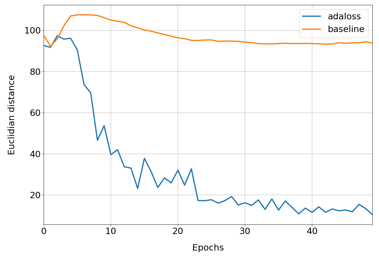
Figure 3: Evolution of the euclidian distance on the CathDet validation set using Adadelta with and without Adaloss.

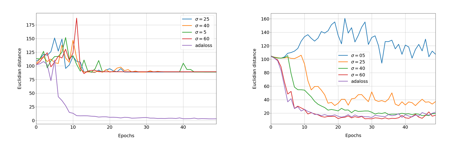
Figure 4: Evolution of the Euclidian distance on the CathDet validation set for multiple fixed values of sigma and Adaloss. Left figure is using the Adam optimizer with a learning rate of $10^{-3}$ and on the right using a learning rate of $10^{-4}$. While the models with fixed sigmas can only train with the lower learning rate, models trained with Adaloss trains faster and better with higher learning rate.

Our first experiment is conducted on a medical dataset of 3300 fluoroscopy scans (X-ray images) annotated with a single landmark which marks the tip of a catheter. We refer to this dataset as “Cathdet”. 3000 images are used for training and 300 are used for testing. The output of the network is a heatmap with resolution of 256x256.

We first examined the benefits of Adaloss in terms of training stability. As setting the learning rate also known to have a significant impact on training stability, a natural comparison to our method is to use an adaptive learning rate method such as Adadelta [33]. However, as illustrated in figure Figure 3, only adapting the learning rate was not sufficient for handling problems with significant sample bias.

In addition to using a smaller learning rate, another possibility could be to increase sigma. However, finding the appropriate value for sigma highly depends on the problem and while using higher sigma certainly helps to stabilize the training, it also increase tolerance to errors in prediction and ends up altering the final accuracy.

We compared these approaches to Adaloss and trained multiple models with different learning rates and different values for sigma (Figure 4). Here, when using the Adam optimizer with a learning rate of $10^{-3}$, models with fixed sigmas are not able to train, even with high values such as $\sigma=40$. When decreasing the learning rate by a factor of 10, models with fixed sigmas no longer diverge, at the cost of slower training and lower accuracy (except for the one with $\sigma=5$ which still could not train). In comparison, models trained with Adaloss can train with both learning rates, and converges faster and better with the higher learning rate. The best non-adaptive method here is using $\sigma=40$. The network which is trained with $\sigma=60$ starts with a better accuracy, but the error starts to increase after a certain number of epochs, due to the excessive tolerance. Table 1 shows best results on testing set for all values of sigmas and Adaloss after 150 epochs. Model trained with Adaloss shows the lowest 1.19 Euclidian distance.

	$\sigma=5$	$\sigma=25$	$\sigma=40$	$\sigma=60$	Adaloss
Dist.	87.05	19.27	8.71	11.46	1.19

Table 1: Euclidian distance on CathDet testing set for multiple values of sigma compared to Adaloss.

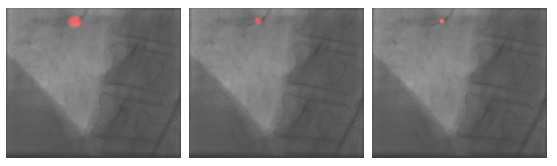
Figure 5: Example of a challenging sample from the validation set. In the early training (left image), the proposed method generates targets with a large variance. At convergence (middle image), target variance becomes much smaller and precisely defines the tip of the catheter. Right image presents the ground truth catheter tip position.

Finally, we investigated the evolution of the standard deviation across the training (Figure 6). After 60 epochs, the model converges and the standard deviation stops decreasing. This shows that Adaloss has found the optimal value for sigma for this problem. Here, the value of the final standard deviation is about 5 pixels. We found this value to be representative of the variance in the ground truth annotations of the tip of the catheter. The variance here is very small as the target defines a precise point on the image.

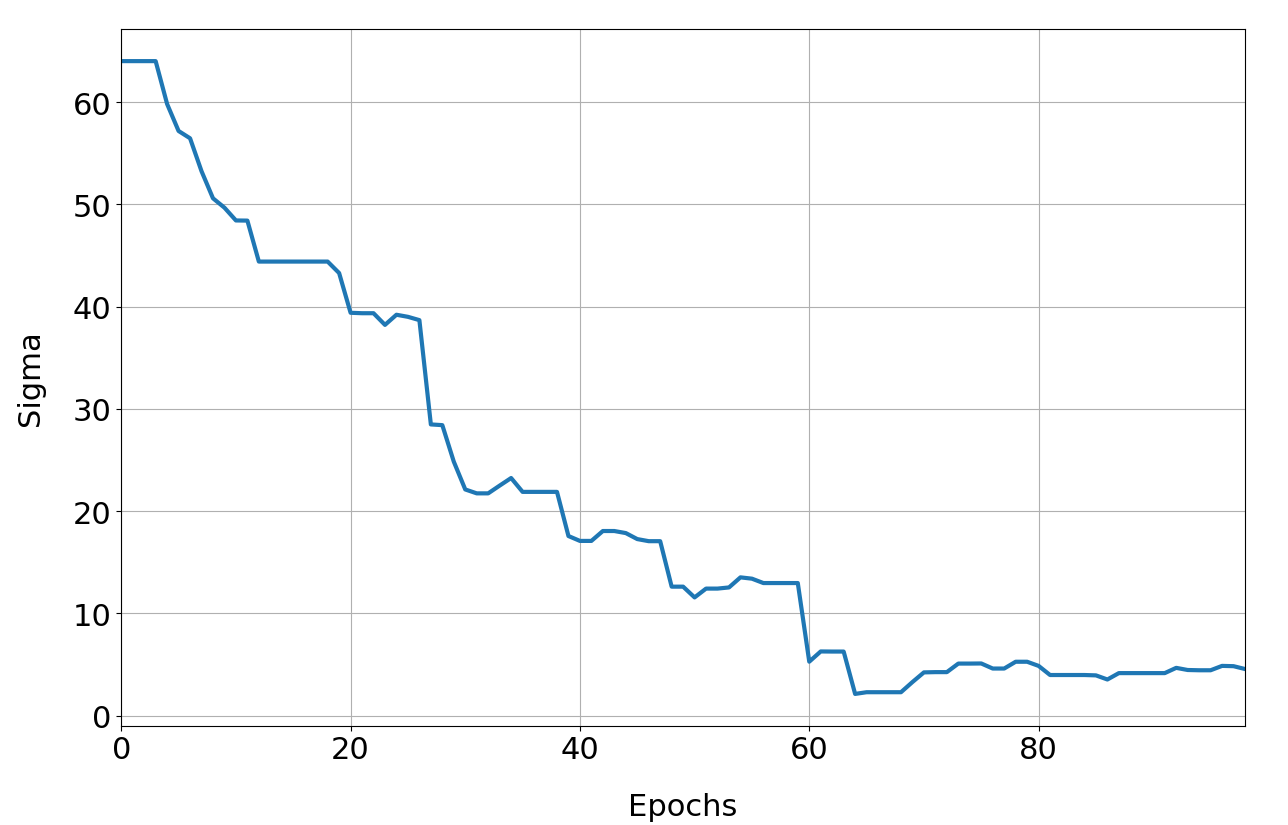
Figure 6: Evolution of the standard deviation during the training of the catheter tip detection model. At convergence, sigma stops decreasing, showing that it has reached the optimal value (Here around 5 pixels). This final value may represent the variance in the annotation.

Exploring the kernel smoothness

Recently, Ruderman et al. [29] explored how filter smoothness is an important factor for determining the stability of convolutional networks to deformation. They presented a method for measuring filter smoothness using Normalized Total Variation (NTV) and show how this metric correlates with the ability of the network to learn the deformation bias. We computed this metric on best networks with and without Adaloss and reported the NTV scores in Table 2. Model trained with Adaloss presents a much smaller NTV (2.80 vs 3.03), indicating a potential impact of using Adaloss on filter smoothness.

	Fixed sigma	Adaloss
All	3.03	2.80
Last	1.83	1.68

Table 2: Normalized Total Variation (NTV) score with and without Adaloss. ‘all’ represents the aggregate NTV on all the layers, and ‘last’ the NTV on the final convolutional layer. Model trained using Adaloss has smoother filters, indicating potential improvement in network stability.

4.3 Single instances of multiple landmarks

We conducted our second experiment on the 300-W dataset [6, 36, 37]. This dataset is an aggregation of five face datasets annotated with 68 landmarks: LFPW [38], AFW [7], HELEN [39], XM2VTS and IBUG. It is often used as a benchmark dataset for evaluating facial feature localization methods [40, 41, 42]. We followed the same splitting as in [19, 31, 42, 43], and used all training samples from LFPW and HELEN and the whole AFW dataset for training. Testing samples from LFPW and HELEN are used as the “common” testing set, while IBUG testing set is considered as “challenging”. This splitting results in a training set of 3148 images, a common testing set of 554 images and a challenging set of 135 images. The union of the common and the challenging set is used as the “full” testing set.

When working on multi-landmarks problems, the difficulty resides in the difference between the landmarks. For a given set of landmarks, some of them might have well defined features and a small variance in the annotation (e.g. eye landmarks) while some others might have varying features (this is the case for the mouth, which could be either open or closed), or may have a large variance in the annotation as for the jaw which defines a broad region of the face.

Adaloss addresses this issue by using different standard deviations for different landmarks. Here, the update rule is the same as for the single landmark case, except that the loss is computed per landmark, meaning that at a given step in the training, one landmark can see its standard deviation decrease while the other ones might not. To further increase the impact of having varying target distributions, we normalize each target heatmap with its mean.

Figure 7 shows how Adaloss evolves during training. We aggregated the evolution of the standard deviation for different regions. Jaw and eyebrows are difficult landmarks: jaw landmarks suffer from significant variance in the annotations and eyebrows landmarks are very sensitive to face orientation. It is interesting to see that the standard deviation decreased slowly for these landmarks and kept a relatively high standard deviation at convergence. On the other hand, the standard deviation decreased faster for the mouth landmarks, and even faster and lower for the eyes and nose landmarks, which are less subject to variance in annotations.

These observations suggest that Adaloss was indeed able to adapt the standard deviation for the landmarks with regard to their difficulty.

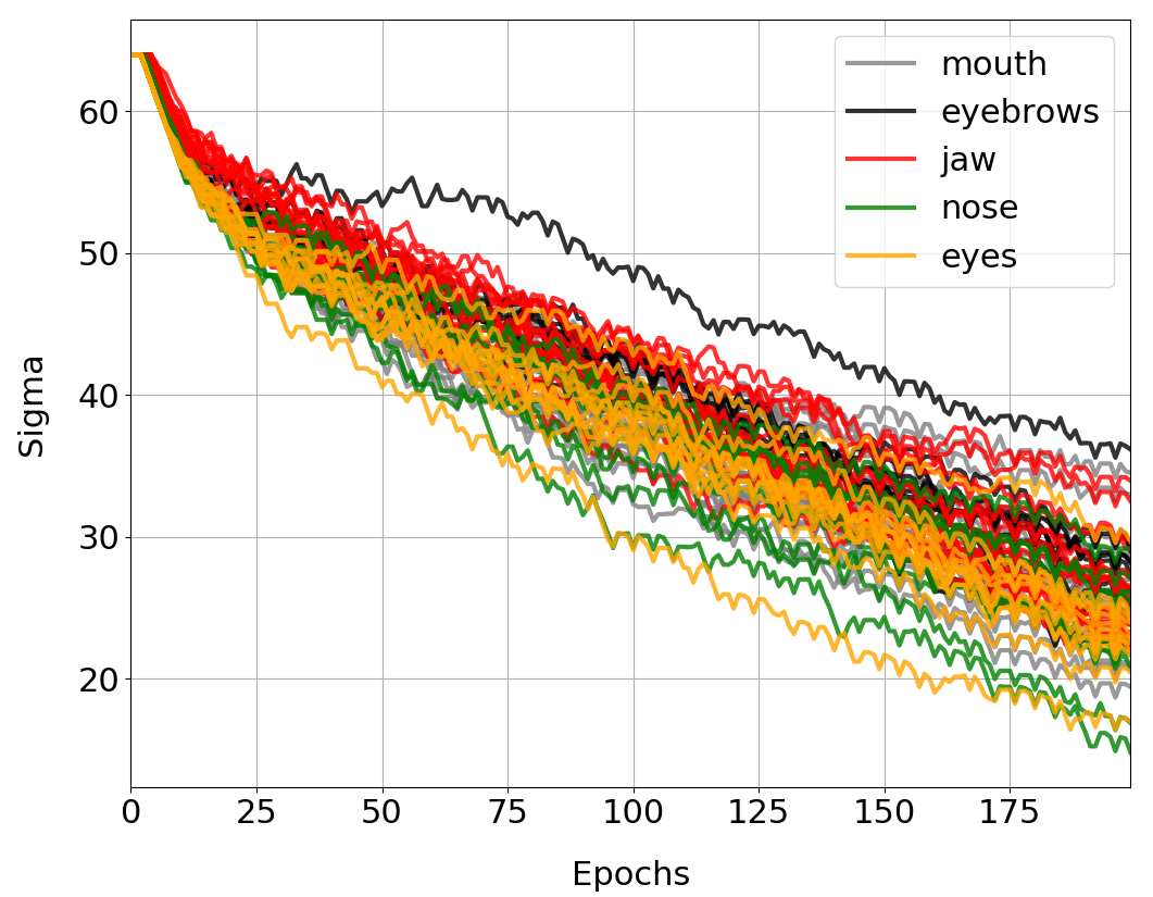
Figure 7: Evolution of the standard deviation for landmarks in different regions. Well defined regions such as eyes and nose decrease fast while locations subject to occlusions or variance in annotations decrease slower.

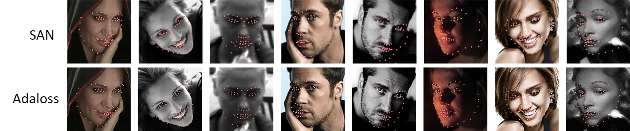
Figure 8: Example of difficult samples from the challenging dataset. Our method is more robust to occlusions and better captures local features even at low resolution, or in bad lighting conditions.

We trained our Dense U-Net end-to-end minimizing the Mean Squared Error (MSE) using the Adam optimizer [12] with an initial learning rate of $10^{-4}$. We augmented the training set using rotations from $-30$ to $+30$ degrees. We used the ground truth bounding box to prepare the input for our network at a resolution of $256$x$256$. Table 3 compares the normalized mean errors (NME) with recent state-of-the-art methods. Following these works, we use the inter-ocular distance (IOD) to normalize the mean error. Our network trained with Adaloss shows the best results on all testing sets. On the common test set, our approach outperforms the previous best method with a NME of 2.76 vs $3.28$. On the challenging set, our method reached a NME of 5.61 vs $6.60$. Overall NME on the full test is 3.31 vs $3.98$. We also compare our approach with the widely used Dlib [44], which was also initialized using the provided ground truth bounding box from 300W. Again, our approach presents better results on all testing sets, and especially on the challenging one (5.61 vs $19.39$), showing the robustness of our approach. Figure 8 shows qualitative results from our method compared to [19] on difficult samples from the challenging set. Results from [19] were generated using provided code and models. Our method was able to better address the occlusion issues and learned a better model of the face.

Method	Common	Challenging	Full
LBF [45]	4.95	11.98	6.32
CFSS [42]	4.73	9.98	5.76
MDM [41]	4.83	10.14	5.88
TCDCN [46]	4.80	8.60	5.54
Two-Stage [43]	4.36	7.42	4.96
RDR [47]	5.03	8.95	5.80
Pose-Invariant [40]	5.43	9.88	6.30
RCN [18]	4.20	7.78	4.90
SAN [19]	3.34	6.60	3.98
CPM + SBR [31]	3.28	7.58	4.10
Dlib [44]	4.38	19.39	7.32
Adaloss	2.76	5.61	3.31

Table 3: Normalized mean errors (NME) on the 300-W dataset. Proposed approach shows best results on all testing sets.

4.4 Multiple instances of multiple landmarks

For our final experiment, we used the MICCAI 2015 challenge EndoVis dataset [48], a high resolution ($576$ x $720$) intra-operative dataset of laparoscopic images with annotated instruments [49].

In this experiment, we focused on only two landmarks: “Right Clasper” and “Left Clasper”, which correspond to the extremities of the tool (Figure 9). These landmarks are the most important to track as they define the parts of the tool that are interacting with the tissues. Here again, landmarks are represented with Gaussian heatmaps, but in this case, there can be multiple Gaussians in each target heatmap, since multiple instances of a particular tool type may appear in the frames simultaneously.

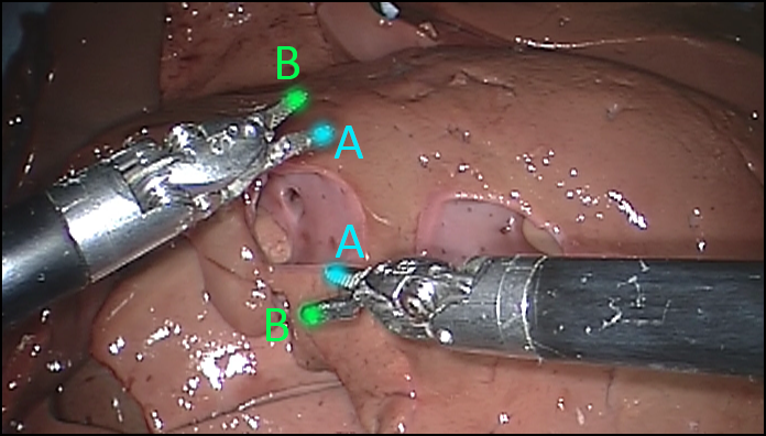
Figure 9: Example of multiple instances of a Needle Driver from the testing set. Landmarks (A) define the Right Clasper and landmarks (B) the Left Clasper.

When detecting multiple instances of a landmark on a given image, it is not possible to use argmax anymore to get the final coordinates. We first applied a median filter with a kernel dimension of [$7$, $7$] followed by non-maxima suppression (NMS) using a window size of $10$ pixels. Finally, the centers of the remaining clusters of points correspond to the localization of the detected landmarks.

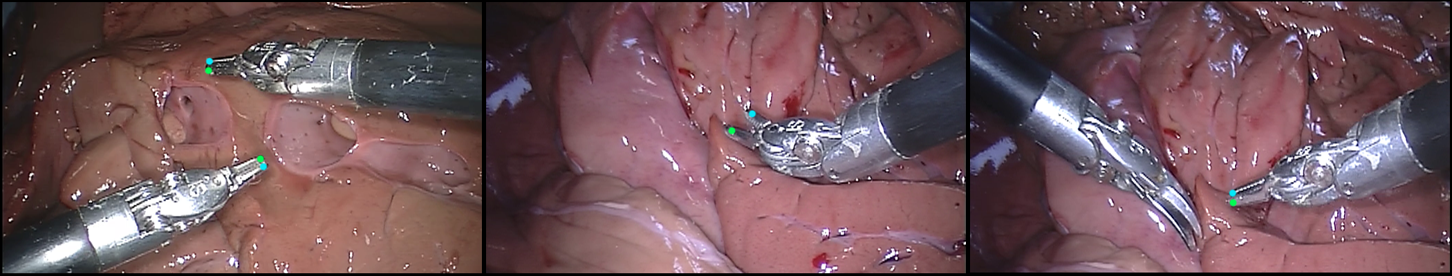
Figure 10: Results from the proposed approach on both EndoVis testing set. Left and center images show results from the testing set without Scissors. Right image shows a result from the full testing set where the Curved Scissor was not misinterpreted as a Needle Driver.

The EndoVis dataset provides images of two different tools: “Curved Scissor” and “Needle Driver”. Current state-of-the-art method for detecting instruments in endoscopic images uses a multi-stage approach. It firsts locates joints and association between joints using a detection network, then it refines these joints through a regression network and then retrieves the final location using maximum bipartite graph matching [49]. While this approach performs landmark detection on multiple instruments with no distinction, it is often desirable to distinguish one instrument from another.

We trained our network end-to-end minimizing the Mean Squared Error (MSE) using the Adam optimizer [12] with an initial learning rate of $10^{-3}$. We computed Precision, Recall and Euclidian distance of our predictions on the testing set of 910 images. This testing set is composed of images with both curved scissors and needle drivers, for which there may be multiple instances in the same frame. Results can be seen in Table 4. Our model performs a left clasper precision of 90.50% with a recall of 95.56% on the needle driver. In comparison, the multi-stage approach from [49] performs a left clasper precision of $86.65\%$ with a recall of $86.28\%$ on both tools with no distinction.

One important thing to note is that the curved scissor is not present in the training set. Our end-to-end network was thus trained to detect only needle drivers. To investigate the robustness of our network and its ability to distinguish tools, we evaluated our approach on two subsets, one composed of 308 images with needle driver only, and other composed of 301 samples where each image contains both needle drivers and curved scissors. On the first subset, our model detected the claspers with a mean precision of $96.56\%$ across all landmarks. On the second subset, the mean precision dropped to $92.16\%$. While this decrease in precision is expected due to the presence of unseen tools, it is interesting to see that the mean precision is still over $90\%$, showing that our model was able to learn discriminative features to distinguish different instruments. Qualitative results from these subsets can be found in Figure 10.

	Left Clasper	Right Clasper
No Scissor	$93.18$ / $98.86$ / $7.23$	$96.59$ / $94.26$ / $6.38$
With Scissors	$98.02$ / $97.10$ / $7.21$	$97.37$ / $87.23$ / $6.56$
Full set	$95.56$ / $90.50$ / $6.83$	$96.38$ / $81.20$ / $6.61$

Table 4: Quantitative results of the Adaloss model on different testing set of EndoVis: Recall (%) / Precision (%) / Euclidian distance (px).

5 Conclusion

We presented a novel, application-independent approach, “Adaloss”, for training deep neural networks for landmark localization. Our method systematically increases the problem difficulty during training and as a result implicitly creates a training curriculum. It addresses the sample bias problem in training, which is arguably the main limitation of the existing heatmap regression methods. We demonstrated the effectiveness of our method on three challenging domains: detecting catheter tips in X-ray images, localizing surgical instruments in endoscopy images, and facial feature localization on in-the-wild images, where we significantly advance the state-of-the-art. While progressively updating the objective function for landmark regression appears to be effective, the viability of such a method has not been explored for other regression or classification tasks and is yet open to discussion.

References

- [1] Maria Jabon, Jeremy Bailenson, Emmanuel Pontikakis, Leila Takayama, and Clifford Nass. Facial expression analysis for predicting unsafe driving behavior. IEEE Pervasive Computing, 10(4):84–95, 2011.
- [2] Tomasz Grzejszczak, Michal Kawulok, and Adam Galuszka. Hand landmarks detection and localization in color images. Multimedia Tools and Applications, 75(23):16363–16387, 2016.
- [3] Y. Zheng, M. John, R. Liao, A. Nottling, J. Boese, J. Kempfert, T. Walther, G. Brokmann, and D. Comaniciu. Automatic aorta segmentation and valve landmark detection in c-arm ct: application to aortic valve implantation. IEEE Trans. on Medical Imaging, 31(12), 2012.
- [4] J. Shotton, R. Girshick, A. Fitzgibbon, T. Sharp, M. Cook, M. Finocchio, R. Moore, P. Kohli, A. Criminisi, A. Kipman, and A. Blake. Efficient human pose estimation from single depth images. T-PAMI, 35(12):2821–2840, 2013.
- [5] Xiaofei Du, Thomas Kurmann, Ping-Lin Chang, Maximilian Allan, Sebastien Ourselin, Raphael Sznitman, John D. Kelly, and Danail Stoyanov. Articulated multi-instrument 2-d pose estimation using fully convolutional networks. IEEE Trans. on Medical Imaging, 37:1276–1287, 2018.
- [6] Christos Sagonas, Epameinondas Antonakos, Georgios Tzimiropoulos, Stefanos P. Zafeiriou, and Maja Pantic. 300 faces in-the-wild challenge: database and results. Image and Vision Comput., 47:3–18, 2016.
- [7] Shuo Yang, Ping Luo, Chen Change Loy, and Xiaoou Tang. Wider face: A face detection benchmark. In IEEE Conference on Computer Vision and Pattern Recognition (CVPR), 2016.
- [8] Mykhaylo Andriluka, Leonid Pishchulin, Peter Gehler, and Bernt Schiele. 2d human pose estimation: New benchmark and state of the art analysis. In IEEE Conference on Computer Vision and Pattern Recognition (CVPR), June 2014.
- [9] Benjamin Sapp and Ben Taskar. Modec: Multimodal decomposable models for human pose estimation. In In Proc. CVPR, 2013.
- [10] Olaf Ronneberger, Philipp Fischer, and Thomas Brox. U-net: Convolutional networks for biomedical image segmentation. CoRR, abs/1505.04597, 2015.
- [11] Sergey Ioffe and Christian Szegedy. Batch normalization: Accelerating deep network training by reducing internal covariate shift. CoRR, abs/1502.03167, 2015.
- [12] Diederik P. Kingma and Jimmy Ba. Adam: A method for stochastic optimization. In ICLR, 2015.
- [13] Vinod Nair and Geoffrey E. Hinton. Rectified linear units improve restricted boltzmann machines. In Int. Conf. on Machine Learning, 2010.
- [14] Zhanpeng Zhang, Ping Luo, Chen Change Loy, and Xiaoou Tang. Learning deep representation for face alignment with auxiliary attributes. IEEE PAMI, 38(5):918–930, May 2016.
- [15] Yue Wu, Tal Hassner, Kanggeon Kim, G. Medioni, and P. Natarajan. Facial landmark detection with tweaked convolutional neural networks. T-PAMI, 40(12), 2017.
- [16] Jonathan Tompson, Arjun Jain, Yann LeCun, and Christoph Bregler. Joint training of a convolutional network and a graphical model for human pose estimation. CoRR, abs/1406.2984, 2014.
- [17] Alejandro Newell, Kaiyu Yang, and Jia Deng. Stacked hourglass networks for human pose estimation. In Bastian Leibe, Jiri Matas, Nicu Sebe, and Max Welling, editors, ECCV, pages 483–499, 2016.
- [18] S. Honari, P. Molchanov, S. Tyree, P. Vincent, C. Pal, and J. Kautz. Improving landmark localization with semi-supervised learning. In CVPR, 2018.
- [19] Xuanyi Dong, Yan Yan, Wanli Ouyang, and Yi Yang. Style aggregated network for facial landmark detection. In Proceedings of the IEEE Conference on Computer Vision and Pattern Recognition (CVPR), pages 379–388, June 2018.
- [20] X. Dong, S. Yu, X Weng, S. Wei, Y. Yang, and Y. Sheikh. Supervision-by-registration: An unsupervised approach to improve the precision of facial landmark detectors. In CVPR, 2018.
- [21] Shih-En Wei, Varun Ramakrishna, Takeo Kanade, and Yaser Sheikh. Convolutional pose machines. In CVPR, 2016.
- [22] Wei Yang, Shuang Li, Wanli Ouyang, Hongsheng Li, and Xiaogang Wang. Learning feature pyramids for human pose estimation. CoRR, abs/1708.01101, 2017.
- [23] Xiao Chu, Wei Yang, Wanli Ouyang, Cheng Ma, Alan L. Yuille, and Xiaogang Wang. Multi-context attention for human pose estimation. CoRR, abs/1702.07432, 2017.
- [24] Lipeng Ke, Ming-Ching Chang, Honggang Qi, and Siwei Lyu. Multi-scale structure-aware network for human pose estimation. CoRR, abs/1803.09894, 2018.
- [25] T.A. Lampert, A. Stumpf, and P. Garcarski. An empirical study into annotator agreement, ground truth estimation, and algorithm evaluation. IEEE Trans. on Image Processing, 25, 2016.
- [26] Christoph Lassner, Javier Romero, Martin Kiefel, Federica Bogo, Michael J. Black, and Peter V. Gehler. Unite the people: Closing the loop between 3d and 2d human representations. In IEEE Conf. on Computer Vision and Pattern Recognition (CVPR), July 2017.
- [27] Adrian Davison, Claudia Lindner, Daniel C Perry, Weisang Luo, and Timothy Cootes. Landmark localisation in radiographs using weighted heatmap displacement voting. In MICCAI Workshop on Comp. Methods and Clinical Apps. in Musculoskeletal Imaging, 2018.
- [28] Alison Q O’Neil, Antanas Kascenas, Joseph Henry, Daniel Wyeth, Matthew Shepherd, Erin Beveridge, Lauren Clunie, Carrie Sansom, Evelina Šeduikytė, Keith Muir, and Ian Poole. Attaining human-level performance with atlas location autocontext for anatomical landmark detection in 3d ct data, 2018.
- [29] Avraham Ruderman, Neil Rabinowitz, Ari S. Morcos, and Daniel Zoran. Learned deformation stability in convolutional neural networks, 2018.
- [30] Alexander Toshev and Christian Szegedy. Deeppose: Human pose estimation via deep neural networks. CoRR, abs/1312.4659, 2013.
- [31] Xuanyi Dong, Shoou-I Yu, Xinshuo Weng, Shih-En Wei, Yi Yang, and Yaser Sheikh. Supervision-by-Registration: An unsupervised approach to improve the precision of facial landmark detectors. In Proceedings of the IEEE Conference on Computer Vision and Pattern Recognition (CVPR), pages 360–368, June 2018.
- [32] Ian Goodfellow, Jean Pouget-Abadie, Mehdi Mirza, Bing Xu, David Warde-Farley, Sherjil Ozair, Aaron Courville, and Yoshua Bengio. Generative adversarial nets. In Z. Ghahramani, M. Welling, C. Cortes, N. D. Lawrence, and K. Q. Weinberger, editors, Advances in Neural Information Processing Systems 27, pages 2672–2680. Curran Associates, Inc., 2014.
- [33] Matthew D. Zeiler. Adadelta: An adaptive learning rate method, 2012.
- [34] Adam Paszke, Sam Gross, Soumith Chintala, Gregory Chanan, Edward Yang, Zachary DeVito, Zeming Lin, Alban Desmaison, Luca Antiga, and Adam Lerer. Automatic differentiation in pytorch. In NIPS-W, 2017.
- [35] Xiaomeng Li, Hao Chen, Xiaojuan Qi, Qi Dou, Chi-Wing Fu, and Pheng-Ann Heng. H-denseunet: Hybrid densely connected unet for liver and liver tumor segmentation from CT volumes. CoRR, abs/1709.07330, 2017.
- [36] C. Sagonas, G. Tzimiropoulos, S. Zafeiriou, and M. Pantic. A semi-automatic methodology for facial landmark. In AMFG, 2013.
- [37] C. Sagonas, G. Tzimiropoulos, S. Zafeiriou, and M. Pantic. 300 faces in-the-wild challenge: The first facial landmark localization challenge. In ICCV-W, 2013.
- [38] Peter N. Belhumeur, David W. Jacobs, David J. Kriegman, and Neeraj Kumar. Localizing parts of faces using a consensus of exemplars. IEEE Trans. Pattern Anal. Mach. Intell., 35(12):2930–2940, 2013.
- [39] Vuong Le, Jonathan Brandt, Zhe Lin, Lubomir D. Bourdev, and Thomas S. Huang. Interactive facial feature localization. In Computer Vision - ECCV 2012 - 12th European Conference on Computer Vision, Florence, Italy, October 7-13, 2012, Proceedings, Part III, pages 679–692, 2012.
- [40] Amin Jourabloo, Mao Ye, Xiaoming Liu, and Liu Ren. Pose-invariant face alignment with a single CNN. In IEEE International Conference on Computer Vision, ICCV 2017, Venice, Italy, October 22-29, 2017, pages 3219–3228, 2017.
- [41] George Trigeorgis, Patrick Snape, Mihalis A. Nicolaou, Epameinondas Antonakos, and Stefanos Zafeiriou. Mnemonic descent method: A recurrent process applied for end-to-end face alignment. In 2016 IEEE Conference on Computer Vision and Pattern Recognition, CVPR 2016, Las Vegas, NV, USA, June 27-30, 2016, pages 4177–4187, 2016.
- [42] Shizhan Zhu, Cheng Li, Chen Change Loy, and Xiaoou Tang. Face alignment by coarse-to-fine shape searching. In IEEE Conference on Computer Vision and Pattern Recognition, CVPR 2015, Boston, MA, USA, June 7-12, 2015, pages 4998–5006, 2015.
- [43] Jiangjing Lv, Xiaohu Shao, Junliang Xing, Cheng Cheng, and Xi Zhou. A deep regression architecture with two-stage re-initialization for high performance facial landmark detection. In Proceedings of the IEEE conference on computer vision and pattern recognition, 2017.
- [44] Davis E. King. Dlib-ml: A machine learning toolkit. J. Mach. Learn. Res., 10:1755–1758, December 2009.
- [45] Shaoqing Ren, Xudong Cao, Yichen Wei, and Jian Sun. Face alignment via regressing local binary features. IEEE Trans. Image Processing, 25(3):1233–1245, 2016.
- [46] Zhanpeng Zhang, Ping Luo, Chen Change Loy, and Xiaoou Tang. Facial landmark detection by deep multi-task learning. In Computer Vision - ECCV 2014 - 13th European Conference, Zurich, Switzerland, September 6-12, 2014, Proceedings, Part VI, pages 94–108, 2014.
- [47] Shengtao Xiao, Jiashi Feng, Luoqi Liu, Xuecheng Nie, Wei Wang, Shuicheng Yan, and Ashraf A. Kassim. Recurrent 3d-2d dual learning for large-pose facial landmark detection. In IEEE International Conference on Computer Vision, ICCV 2017, Venice, Italy, October 22-29, 2017, pages 1642–1651, 2017.
- [48] Endoscopic vision challenge: Instrument segmentation and tracking, 2015.
- [49] Xiaofei Du, Thomas Kurmann, Ping-Lin Chang, Max Allan, Sébastien Ourselin, Raphael Sznitman, John D. Kelly, and Danail Stoyanov. Articulated multi-instrument 2-d pose estimation using fully convolutional networks. IEEE Trans. Med. Imaging, 37(5):1276–1287, 2018.