An Incremental Approach to Online Dynamic Mode Decomposition for Time-Varying Systems with Applications to EEG Data Modeling thanks: This work has been supported by NSF Award IIS-1734272.

Mustaffa Alfatlawi                        Vaibhav Srivastava Electrical and Computer Engineering Department, College of Engineering, Michigan State University, East Lansing, MI (alfatlaw@msu.edu, vaibhav@egr.msu.edu ).
Abstract

Dynamic Mode Decomposition (DMD) is a data-driven technique to identify a low dimensional linear time invariant dynamics underlying high-dimensional data. For systems in which such underlying low-dimensional dynamics is time-varying, a time-invariant approximation of such dynamics computed through standard DMD techniques may not be appropriate. We focus on DMD techniques for such time-varying systems and develop incremental algorithms for systems without and with exogenous control inputs. We build upon the work in [35] to scenarios in which high dimensional data are governed by low dimensional time-varying dynamics. We consider two classes of algorithms that rely on (i) a discount factor on previous observations, and (ii) a sliding window of observations. Our algorithms leverage existing techniques for incremental singular value decomposition and allow us to determine an appropriately reduced model at each time and are applicable even if data matrix is singular. We apply the developed algorithms for autonomous systems to Electroencephalographic (EEG) data and demonstrate their effectiveness in terms of reconstruction and prediction. Our algorithms for non-autonomous systems are illustrated using randomly generated linear time-varying systems.

Keywords: data-driven dynamics, dynamic mode decomposition, time-varying systems, incremental algorithms

1 Introduction

Emergence of low cost sensors and their widespread deployment has led to an unprecedented amount of data. Extraction of actionable information from such plethora of data remains a challenge. It is often the case that a low dimensional dynamical system governs the high-dimensional spatiotemporal sensory data. Dynamic Mode Decomposition (DMD) has emerged as a popular data-driven technique to efficiently compute such low dimensional dynamics [30, 19, 33]. One of the attractive features of the DMD approach is that it requires minimal assumptions on the data. Furthermore, its strong connections with the Koopman operator [29, 23, 24, 25, 17] makes it further appealing and theoretically grounded. The efficacy and simplicity of the DMD has inspired its application in a wide range of areas from fluid dynamics [30, 19] to video processing [10, 32] to epidemiology [28] to neuroscience [3].

For high-dimensional data that is generated by an underlying low dimensional time-varying dynamics, the standard DMD approach may be applicable only locally in time and appropriate time-varying DMD operators can be computed by discounting old data or considering a sliding window of observations [35]. Even in scenarios when underlying dynamics is time-invariant and nonlinear, such time-varying linear approximations have been shown to be very effective [7]. In this paper, we develop incremental methods for the computation of the DMD for time-varying systems and demonstrate the utility of the developed algorithm using Electroencephalographic (EEG) data.

Incremental approaches to DMD refer to methods that allow for efficiently computing the DMD when data is provided sequentially instead of being provided as a batch. The sequential arrival might be due to the inherent nature of the application or it may be used for computational efficiency even if all the data is accessible. One such technique is streaming DMD [13, 12] that first computes the projection of new data on the current orthogonal basis for the range of the data matrix and compares the norm of the difference between the projection and the new data with a threshold. If the difference is larger than the threshold, then it appends the basis with an additional element. Incremental total DMD introduced in [21] applies incremental Singular Value Decomposition (SVD) [1, 2, 26] for incremental computation of dynamic modes and subsequent identification of dominant modes. Unlike the streaming DMD and the total DMD, our focus in this paper is on systems with time-varying dynamics.

Within the context of time-varying systems, an incremental approach is the Online DMD  [35], which adapts the sequential least squares method [16, 15] to incrementally update the DMD computation. The online DMD incrementally computes the DMD operator using the Sherman-Morrison identity [31]. Authors of [35] consider two strategies in their DMD computation to account for time-varying systems: (i) discounting the old data, and (ii) using a sliding window of observations. They also consider DMD for systems with control input [27, 18]. In particular, they extend the DMD with control approach proposed in [27] to develop an online DMD with control algorithm for time-varying system.

In this paper, we build upon the work in [35], and develop incremental SVD based techniques for the computation of the online DMD for time-varying systems. The proposed approach provides access to singular values of the data matrix at each time and hence allows it to determine a reduced order model. For the scenarios in which the high-dimensional data is governed by a low-dimensional dynamics, such reduced order models provide better future prediction accuracy. Furthermore, for scenarios where the Sherman-Morrison identity cannot be applied, e.g., if the data matrix remains singular even after sufficiently long time, the access to singular values allows for efficient computation of appropriate pseudo-inverse. The major contributions of this work are fourfold

  1. (i).

    We leverage incremental SVD techniques to develop two algorithms for the computation of the online DMD for time-varying systems that rely on discounting old data and a sliding window of data, respectively;

  2. (ii).

    We extend both these algorithms to develop incremental SVD based algorithms for the computation of the online DMD with control input for time-varying systems;

  3. (iii).

    We apply our algorithms for the case without control input on an EEG dataset and show their efficacy in reconstructing and predicting error related potential, a slow cortical potential seen in the EEG signal that is elicited by an unexpected outcome;

  4. (iv).

    We apply our algorithms for the case with control input on randomly generated linear time-varying dynamical systems, and demonstrate their efficacy.

The remainder of the paper is organized as follows. In Section 2, we present some background on the DMD for time-invariant and time-varying systems. In Section 3, we present some background for the incremental SVD algorithms. In Section 4, we leverage the incremental SVD algorithms to develop novel incremental DMD algorithms. We apply these algorithms to EEG data in Section 5. We present incremental SVD-based algorithms for online DMD with control and illustrate its utility using numerical examples in Section 6. Finally, we conclude in Section 7.

Notation: We denote the set of real and complex matrices of size n×m𝑛𝑚n\times m by n×msuperscript𝑛𝑚\mathbb{R}^{n\times m} and n×msuperscript𝑛𝑚\mathbb{C}^{n\times m}, respectively. The set of real and complex n𝑛n-dimensional vectors are denoted by nsuperscript𝑛\mathbb{R}^{n} and nsuperscript𝑛\mathbb{C}^{n}, respectively. We denote matrices with bold upper case letters, vectors with bold lower case letters, and scalar with normal lower case letters. We denote the matrix transpose and the matrix conjugate transpose by ()TsuperscriptT(\cdot)^{\text{T}} and ()superscript(\cdot)^{*}, respectively. The kernel and range of a matrix 𝐗𝐗\mathbf{X} are denoted by Ker𝐗Ker𝐗\text{Ker}\mathbf{X}, and Ran𝐗Ran𝐗\text{Ran}\mathbf{X}, respectively.

2 Dynamic Mode Decomposition for Time-Varying Systems

In this section, we recall the DMD setup and describe the time-varying DMD problem that we study in this paper.

2.1 Dynamic Mode Decomposition

Consider the following discrete-time system:

𝐱k+1subscript𝐱𝑘1\displaystyle\mathbf{x}_{k+1} =\displaystyle= 𝐟(𝐱k),𝐟subscript𝐱𝑘\displaystyle\mathbf{f}(\mathbf{x}_{k}), (1)

where 𝐱knsubscript𝐱𝑘superscript𝑛\mathbf{x}_{k}\in\mathbb{R}^{n} is a high-dimensional state vector (n1much-greater-than𝑛1n\gg 1) sampled at tk=kΔtsubscript𝑡𝑘𝑘Δ𝑡t_{k}=k\Delta t, k{1,,(m+1)}𝑘1𝑚1k\in\{1,\dots,(m+1)\}, and 𝐟𝐟\mathbf{f} is an unknown map which describes the evolution of the state vector between two subsequent sampling times. Suppose that the evolution of the high-dimensional state 𝐱𝐱\mathbf{x} is governed by some underlying low-dimensional dynamics. Then, the DMD computes a data-driven linear approximation to the system (1) as follows [19, 33].

Consider a collection of (m+1)𝑚1(m+1) sequential measurements arranged in the following two datasets:

𝐗=[𝐱1𝐱2𝐱m],𝐘=[𝐱2𝐱3𝐱m+1].formulae-sequence𝐗matrixsubscript𝐱1subscript𝐱2subscript𝐱𝑚𝐘matrixsubscript𝐱2subscript𝐱3subscript𝐱𝑚1\displaystyle\mathbf{X}=\begin{bmatrix}\mathbf{x}_{1}&\mathbf{x}_{2}&\cdots&\mathbf{x}_{m}\end{bmatrix},\mathbf{Y}=\begin{bmatrix}\mathbf{x}_{2}&\mathbf{x}_{3}&\cdots&\mathbf{x}_{m+1}\end{bmatrix}.

Let the projection of 𝐗𝐗\mathbf{X} onto its leading r𝑟r singular vectors be 𝐗¯=𝐔¯x𝚺¯x𝐕¯x¯𝐗subscript¯𝐔𝑥subscript¯𝚺𝑥superscriptsubscript¯𝐕𝑥\bar{\mathbf{X}}=\bar{\mathbf{U}}_{x}\bar{\mathbf{\Sigma}}_{x}\bar{\mathbf{V}}_{x}^{*} , where r𝑟r is the targeted dimension of the underlying low-dimensional dynamical system, 𝐔¯xn×rsubscript¯𝐔𝑥superscript𝑛𝑟\bar{\mathbf{U}}_{x}\in\mathbb{C}^{n\times r}, 𝐕¯xr×msubscript¯𝐕𝑥superscript𝑟𝑚\bar{\mathbf{V}}_{x}\in\mathbb{C}^{r\times m}, and 𝚺¯x=diag{σ1,,σr}r×rsubscript¯𝚺𝑥diagsubscript𝜎1subscript𝜎𝑟superscript𝑟𝑟\bar{\mathbf{\Sigma}}_{x}=\text{diag}\{\sigma_{1},\dots,\sigma_{r}\}\in\mathbb{C}^{r\times r}. Then, the DMD framework approximates the dynamics (1) by

𝐱k+1=𝐀¯𝐱k,subscript𝐱𝑘1¯𝐀subscript𝐱𝑘\mathbf{x}_{k+1}=\bar{\mathbf{A}}\mathbf{x}_{k},

where 𝐀¯n×n¯𝐀superscript𝑛𝑛\bar{\mathbf{A}}\in\mathbb{R}^{n\times n} is called the DMD operator and is given by

𝐀¯=𝐘𝐕¯x𝚺¯x1𝐔¯x.¯𝐀𝐘subscript¯𝐕𝑥superscriptsubscript¯𝚺𝑥1superscriptsubscript¯𝐔𝑥\bar{\mathbf{A}}=\mathbf{Y}\bar{\mathbf{V}}_{x}\bar{{\mathbf{\Sigma}}}_{x}^{-1}\bar{{\mathbf{U}}}_{x}^{*}. (2)

Let the projection of the state 𝐱𝐱\mathbf{x} and the DMD operator 𝐀¯¯𝐀\bar{\mathbf{A}} onto the space spanned by leading r𝑟r singular vectors of 𝐗𝐗\mathbf{X} be 𝐱~k=𝐔¯𝐱ksubscript~𝐱𝑘superscript¯𝐔subscript𝐱𝑘\tilde{\mathbf{x}}_{k}=\bar{\mathbf{U}}^{\ast}\mathbf{x}_{k} and

𝐀~=𝐔¯x𝐀¯𝐔¯x=𝐔¯x𝐘𝐕¯x𝚺¯x1,~𝐀superscriptsubscript¯𝐔𝑥¯𝐀subscript¯𝐔𝑥superscriptsubscript¯𝐔𝑥𝐘subscript¯𝐕𝑥superscriptsubscript¯𝚺𝑥1\tilde{\mathbf{A}}=\bar{\mathbf{U}}_{x}^{*}\bar{\mathbf{A}}\bar{\mathbf{U}}_{x}=\bar{\mathbf{U}}_{x}^{*}\mathbf{Y}\bar{\mathbf{V}}_{x}\bar{{\mathbf{\Sigma}}}_{x}^{-1},

respectively. Then, the approximation to the underlying r𝑟r-dimensional dynamics is

𝐱~k+1=𝐀~𝐱~k.subscript~𝐱𝑘1~𝐀subscript~𝐱𝑘\tilde{\mathbf{x}}_{k+1}=\tilde{\mathbf{A}}\tilde{\mathbf{x}}_{k}. (3)

Let 𝚲𝚲\mathbf{\Lambda} be the diagonal matrix of the eigenvalues of 𝐀~~𝐀\tilde{\mathbf{A}} and 𝐖𝐖\mathbf{W} be the matrix of the associated eigenvectors such that

𝐀~𝐖=𝐖𝚲.~𝐀𝐖𝐖𝚲\tilde{\mathbf{A}}\mathbf{W}=\mathbf{W}\mathbf{\Lambda}. (4)

Then, two types of DMD modes can be identified using the eigen-decomposition in (4): the projected DMD modes 𝚽^=𝐔¯x𝐖^𝚽subscript¯𝐔𝑥𝐖\hat{\mathbf{\Phi}}=\bar{\mathbf{U}}_{x}\mathbf{W} and the exact DMD modes 𝚽=𝐘𝐕¯x𝚺¯x1𝐖𝚽𝐘subscript¯𝐕𝑥superscriptsubscript¯𝚺𝑥1𝐖\mathbf{\Phi}=\mathbf{Y}\bar{\mathbf{V}}_{x}\bar{{\mathbf{\Sigma}}}_{x}^{-1}\mathbf{W} [33]. Either of these DMD modes and the associated eigenvalues describe the evolution of the high-dimensional system using low-dimensional dynamics (3).

2.2 Dynamic Mode Decomposition with Control

Consider the following non-autonomous discrete-time system:

𝐱k+1subscript𝐱𝑘1\displaystyle\mathbf{x}_{k+1} =\displaystyle= 𝐟c(𝐱k,𝜸k),superscript𝐟𝑐subscript𝐱𝑘subscript𝜸𝑘\displaystyle\mathbf{f}^{c}(\mathbf{x}_{k},\boldsymbol{\gamma}_{k}), (5)

where 𝐱knsubscript𝐱𝑘superscript𝑛\mathbf{x}_{k}\in\mathbb{R}^{n} is a high-dimensional state vector (n1much-greater-than𝑛1n\gg 1) sampled at tk=kΔtsubscript𝑡𝑘𝑘Δ𝑡t_{k}=k\Delta t, k{1,,(m+1)}𝑘1𝑚1k\in\{1,\dots,(m+1)\}, and fcsuperscript𝑓𝑐f^{c} is an unknown time-varying map which describes the evolution of the state vector between two subsequent sampling times, and 𝜸klsubscript𝜸𝑘superscript𝑙\boldsymbol{\gamma}_{k}\in\mathbb{R}^{l} is the exogenous input. Then, the Dynamic Mode Decomposition with Control (DMDc) computes a data-driven linear approximation to the system (5) as follows [27].

Consider a collection of m𝑚m sequential measurements 𝐱insubscript𝐱𝑖superscript𝑛\mathbf{x}_{i}\in\mathbb{R}^{n} and the associated exogeneous inputs 𝜸ilsubscript𝜸𝑖superscript𝑙\boldsymbol{\gamma}_{i}\in\mathbb{R}^{l}, i{1,,m}𝑖1𝑚i\in\{1,\dots,m\}. DMDc approximates the non-autonomous dynamics underlying these measurements by

𝐱k+1=𝐀𝐱k+𝐁𝜸k=𝐆[𝐱k𝜸k],subscript𝐱𝑘1subscript𝐀𝐱𝑘𝐁subscript𝜸𝑘𝐆matrixsubscript𝐱𝑘subscript𝜸𝑘\mathbf{x}_{k+1}=\mathbf{A}\mathbf{x}_{k}+\mathbf{B}\boldsymbol{\gamma}_{k}=\mathbf{G}\begin{bmatrix}\mathbf{x}_{k}\\ \boldsymbol{\gamma}_{k}\end{bmatrix},

where 𝐀n×n𝐀superscript𝑛𝑛\mathbf{A}\in\mathbb{R}^{n\times n} is called the DMD operator, 𝐁n×l𝐁superscript𝑛𝑙\mathbf{B}\in\mathbb{R}^{n\times l} is called the input matrix, and 𝐆=[𝐀𝐁]n×(n+l)𝐆matrix𝐀𝐁superscript𝑛𝑛𝑙\mathbf{G}=\begin{bmatrix}\mathbf{A}&\mathbf{B}\end{bmatrix}\in\mathbb{R}^{n\times(n+l)}. In particular, the DMDc algorithm constructs matrices 𝐗=[𝐱1𝐱m1]𝐗matrixsubscript𝐱1subscript𝐱𝑚1\mathbf{X}=\begin{bmatrix}\mathbf{x}_{1}&\cdots&\mathbf{x}_{m-1}\end{bmatrix}, 𝐘=[𝐱2𝐱m]𝐘matrixsubscript𝐱2subscript𝐱𝑚\mathbf{Y}=\begin{bmatrix}\mathbf{x}_{2}&\cdots&\mathbf{x}_{m}\end{bmatrix}, and 𝚪=[𝜸1𝜸m1]𝚪matrixsubscript𝜸1subscript𝜸𝑚1\mathbf{\Gamma}=\begin{bmatrix}\boldsymbol{\gamma}_{1}&\cdots&\boldsymbol{\gamma}_{m-1}\end{bmatrix}. Let 𝐗c=[𝐗𝚪](n+l)×(m1)superscript𝐗𝑐matrix𝐗𝚪superscript𝑛𝑙𝑚1\mathbf{X}^{c}=\begin{bmatrix}\mathbf{X}\\ \mathbf{\Gamma}\end{bmatrix}\in\mathbb{R}^{(n+l)\times(m-1)}, and 𝐗c=𝐔c𝚺c𝐕csuperscript𝐗𝑐superscript𝐔𝑐superscript𝚺𝑐superscript𝐕𝑐\mathbf{X}^{c}=\mathbf{U}^{c}\mathbf{\Sigma}^{c}\mathbf{V}^{c*} be its singular value decomposition, where 𝐔c(n+l)×(n+l)superscript𝐔𝑐superscript𝑛𝑙𝑛𝑙\mathbf{U}^{c}\in\mathbb{C}^{(n+l)\times(n+l)}, 𝚺c(n+l)×(n+l)superscript𝚺𝑐superscript𝑛𝑙𝑛𝑙\mathbf{\Sigma}^{c}\in\mathbb{C}^{(n+l)\times(n+l)}, and 𝐕c(m1)×(n+l)superscript𝐕𝑐superscript𝑚1𝑛𝑙\mathbf{V}^{c}\in\mathbb{C}^{(m-1)\times(n+l)}.

The DMDc algorithm estimates 𝐆𝐆\mathbf{G} by

𝐆=𝐘𝐕c(𝚺c)1𝐔c.𝐆superscript𝐘𝐕𝑐superscriptsuperscript𝚺𝑐1superscript𝐔𝑐\mathbf{G}=\mathbf{Y}\mathbf{V}^{c}(\mathbf{\Sigma}^{c})^{-1}\mathbf{U}^{c*}.

Finally, 𝐔csuperscript𝐔𝑐\mathbf{U}^{c*} can be written in a partitioned form of 𝐔c=[𝐔ca𝐔cb]superscript𝐔𝑐matrixsuperscript𝐔subscript𝑐𝑎superscript𝐔subscript𝑐𝑏\mathbf{U}^{c*}=\begin{bmatrix}\mathbf{U}^{c_{a}*}&\mathbf{U}^{c_{b}*}\end{bmatrix}, where 𝐔can×(n+l)superscript𝐔subscript𝑐𝑎superscript𝑛𝑛𝑙\mathbf{U}^{c_{a}}\in\mathbb{C}^{n\times(n+l)} and 𝐔cbl×(n+l)superscript𝐔subscript𝑐𝑏superscript𝑙𝑛𝑙\mathbf{U}^{c_{b}}\in\mathbb{C}^{l\times(n+l)}. Then, the DMDc algorithm computes the matrices 𝐀csuperscript𝐀𝑐\mathbf{A}^{c} and 𝐁csuperscript𝐁𝑐\mathbf{B}^{c} given by

𝐀c=𝐘𝐕c(𝚺c)1𝐔caand𝐁c=𝐘𝐕c(𝚺c)1𝐔cb.formulae-sequencesuperscript𝐀𝑐superscript𝐘𝐕𝑐superscriptsuperscript𝚺𝑐1superscript𝐔subscript𝑐𝑎andsuperscript𝐁𝑐superscript𝐘𝐕𝑐superscriptsuperscript𝚺𝑐1superscript𝐔subscript𝑐𝑏\mathbf{A}^{c}=\mathbf{Y}\mathbf{V}^{c}(\mathbf{\Sigma}^{c})^{-1}\mathbf{U}^{c_{a}*}\quad\text{and}\quad\mathbf{B}^{c}=\mathbf{Y}\mathbf{V}^{c}(\mathbf{\Sigma}^{c})^{-1}\mathbf{U}^{c_{b}*}.

Similar to the case of the DMD, the DMDc algorithm also enables identification of the low-dimensional non-autonomous system underlying the high-dimensional measurements. Assume that the matrix 𝐗csuperscript𝐗𝑐\mathbf{X}^{c} can be approximated by its projection onto the leading p𝑝p singular vectors by 𝐗¯c=𝐔¯c𝚺¯c𝐕¯csuperscript¯𝐗𝑐superscript¯𝐔𝑐superscript¯𝚺𝑐superscript¯𝐕𝑐\bar{\mathbf{X}}^{c}=\bar{\mathbf{U}}^{c}\bar{\mathbf{\Sigma}}^{c}\bar{\mathbf{V}}^{c*}, where 𝐔¯c(n+l)×psuperscript¯𝐔𝑐superscript𝑛𝑙𝑝\bar{\mathbf{U}}^{c}\in\mathbb{C}^{(n+l)\times p}, 𝚺¯cp×psuperscript¯𝚺𝑐superscript𝑝𝑝\bar{\mathbf{\Sigma}}^{c}\in\mathbb{C}^{p\times p}, and 𝐕¯c(m1)×psuperscript¯𝐕𝑐superscript𝑚1𝑝\bar{\mathbf{V}}^{c}\in\mathbb{C}^{(m-1)\times p}, and the matrix 𝐗𝐗\mathbf{X} can be approximated by its projection onto the leading rp𝑟𝑝r\leq p singular vectors by 𝐗¯=𝐔¯𝚺¯𝐕¯¯𝐗¯𝐔¯𝚺superscript¯𝐕\bar{\mathbf{X}}=\bar{\mathbf{U}}\bar{\mathbf{\Sigma}}\bar{\mathbf{V}}^{*}, where 𝐔¯n×r¯𝐔superscript𝑛𝑟\bar{\mathbf{U}}\in\mathbb{C}^{n\times r}, 𝚺¯r×r¯𝚺superscript𝑟𝑟\bar{\mathbf{\Sigma}}\in\mathbb{C}^{r\times r}, and 𝐕¯(m1)×r¯𝐕superscript𝑚1𝑟\bar{\mathbf{V}}\in\mathbb{C}^{(m-1)\times r}. Then, a reduced order model can be represented as follows:

𝐱~k+1=𝐀~c𝐱~k+𝐁~c𝜸k,subscript~𝐱𝑘1superscript~𝐀𝑐subscript~𝐱𝑘superscript~𝐁𝑐subscript𝜸𝑘\displaystyle\tilde{\mathbf{x}}_{k+1}=\tilde{\mathbf{A}}^{c}\tilde{\mathbf{x}}_{k}+\tilde{\mathbf{B}}^{c}{\boldsymbol{\gamma}_{k}},

where the lower-dimensional matrices 𝐀~c𝐑r×rsuperscript~𝐀𝑐superscript𝐑𝑟𝑟\tilde{\mathbf{A}}^{c}\in\mathbf{R}^{r\times r} and 𝐁~c𝐑r×lsuperscript~𝐁𝑐superscript𝐑𝑟𝑙\tilde{\mathbf{B}}^{c}\in\mathbf{R}^{r\times l} can be calculated by:

𝐀~c=𝐔¯𝐘𝐕¯c(𝚺¯c)1𝐔¯ca𝐔¯and𝐁~c=𝐔¯𝐘𝐕c(𝚺c)1𝐔cb.formulae-sequencesuperscript~𝐀𝑐superscript¯𝐔𝐘superscript¯𝐕𝑐superscriptsuperscript¯𝚺𝑐1superscript¯𝐔subscript𝑐𝑎¯𝐔andsuperscript~𝐁𝑐superscript¯𝐔superscript𝐘𝐕𝑐superscriptsuperscript𝚺𝑐1superscript𝐔subscript𝑐𝑏\tilde{\mathbf{A}}^{c}=\bar{\mathbf{U}}^{*}\mathbf{Y}\bar{\mathbf{V}}^{c}(\bar{\mathbf{\Sigma}}^{c})^{-1}\bar{\mathbf{U}}^{c_{a}*}\bar{\mathbf{U}}\quad\text{and}\quad\tilde{\mathbf{B}}^{c}=\bar{\mathbf{U}}^{*}\mathbf{Y}\mathbf{V}^{c}(\mathbf{\Sigma}^{c})^{-1}\mathbf{U}^{c_{b}*}.

2.3 Problem Formulation

In this paper, we study incremental algorithms for the time-varying DMD and DMDc problems defined below.

2.3.1 Time-varying DMD

Consider the time-varying discrete time system of the form

𝐱k+1subscript𝐱𝑘1\displaystyle\mathbf{x}_{k+1} =\displaystyle= 𝐟(tk,𝐱k),𝐟subscript𝑡𝑘subscript𝐱𝑘\displaystyle\mathbf{f}(t_{k},\mathbf{x}_{k}), (6)

where 𝐱knsubscript𝐱𝑘superscript𝑛\mathbf{x}_{k}\in\mathbb{R}^{n} is a high-dimensional state vector (n1much-greater-than𝑛1n\gg 1) sampled at tk=kΔtsubscript𝑡𝑘𝑘Δ𝑡t_{k}=k\Delta t, k{1,,(m+1)}𝑘1𝑚1k\in\{1,\dots,(m+1)\}, and 𝐟𝐟\mathbf{f} is an unknown time-varying map which describes the evolution of the state vector between two subsequent sampling times. Similar to the standard DMD setup, we assume that the high-dimensional dynamics (6) is generated by a low-dimensional time-varying dynamics.

Suppose that, at sampling time tk+1subscript𝑡𝑘1t_{k+1}, we have access to a collection of (w+1)𝑤1(w+1) sequential measurements [𝐱kw+1𝐱kw+2𝐱kw+3𝐱k+1]matrixsubscript𝐱𝑘𝑤1subscript𝐱𝑘𝑤2subscript𝐱𝑘𝑤3subscript𝐱𝑘1\begin{bmatrix}\mathbf{x}_{k-w+1}&\mathbf{x}_{k-w+2}&\mathbf{x}_{k-w+3}&\cdots&\mathbf{x}_{k+1}\end{bmatrix}. Our objective is to design efficient computational techniques to identify the time-varying DMD operator 𝐀ksubscript𝐀𝑘\mathbf{A}_{k} that approximates the system (6) by the following linear time-varying system

𝐱k+1=𝐀k𝐱k,subscript𝐱𝑘1subscript𝐀𝑘subscript𝐱𝑘\displaystyle\mathbf{x}_{k+1}=\mathbf{A}_{k}\mathbf{x}_{k}, (7)

such that the cost function

𝐉(𝐀k)=j=kw+1kρ(kj)(𝐲j𝐀k𝐱j)2,𝐉subscript𝐀𝑘superscriptsubscript𝑗𝑘𝑤1𝑘superscriptnormsuperscript𝜌𝑘𝑗subscript𝐲𝑗subscript𝐀𝑘subscript𝐱𝑗2\displaystyle\mathbf{J}(\mathbf{A}_{k})=\sum_{j=k-w+1}^{k}\left\|\rho^{(k-j)}(\mathbf{y}_{j}-\mathbf{A}_{k}\mathbf{x}_{j})\right\|^{2}, (8)

is minimized, where ρ(0,1]𝜌01\rho\in(0,1] is a discounting factor.

2.3.2 Time-varying DMDc

Consider the following variant of the system in (6)

𝐱k+1subscript𝐱𝑘1\displaystyle\mathbf{x}_{k+1} =\displaystyle= 𝐟c(tk,𝐱k,𝜸k),superscript𝐟𝑐subscript𝑡𝑘subscript𝐱𝑘subscript𝜸𝑘\displaystyle\mathbf{f}^{c}(t_{k},\mathbf{x}_{k},\boldsymbol{\gamma}_{k}), (9)

where fcsuperscript𝑓𝑐f^{c} is an unknown time-varying map which describes the evolution of the state vector between two subsequent sampling times, and 𝜸klsubscript𝜸𝑘superscript𝑙\boldsymbol{\gamma}_{k}\in\mathbb{R}^{l} is the exogenous input.

Assume that, at sampling time 𝐭k+1subscript𝐭𝑘1\mathbf{t}_{k+1}, two collections of sequential measurements are available, one for the system states [𝐱kw+1𝐱kw+2𝐱kw+3𝐱k+1]matrixsubscript𝐱𝑘𝑤1subscript𝐱𝑘𝑤2subscript𝐱𝑘𝑤3subscript𝐱𝑘1\begin{bmatrix}\mathbf{x}_{k-w+1}&\mathbf{x}_{k-w+2}&\mathbf{x}_{k-w+3}&\cdots&\mathbf{x}_{k+1}\end{bmatrix}, and the other one for the exogenous inputs [𝜸kw+1𝜸kw+2𝜸kw+3𝜸k+1]matrixsubscript𝜸𝑘𝑤1subscript𝜸𝑘𝑤2subscript𝜸𝑘𝑤3subscript𝜸𝑘1\begin{bmatrix}\boldsymbol{\gamma}_{k-w+1}&\boldsymbol{\gamma}_{k-w+2}&\boldsymbol{\gamma}_{k-w+3}&\cdots&\boldsymbol{\gamma}_{k+1}\end{bmatrix}. Our objective is to design efficient computational techniques to identify the time-varying DMDc operator 𝐀kcsubscriptsuperscript𝐀𝑐𝑘\mathbf{A}^{c}_{k} and input matrix 𝐁kcsubscriptsuperscript𝐁𝑐𝑘\mathbf{B}^{c}_{k} that approximates the system (9) by the following linear time-varying system

𝐱k+1=𝐀kc𝐱k+𝐁kc𝜸k,subscript𝐱𝑘1subscriptsuperscript𝐀𝑐𝑘subscript𝐱𝑘subscriptsuperscript𝐁𝑐𝑘subscript𝜸𝑘\displaystyle\mathbf{x}_{k+1}=\mathbf{A}^{c}_{k}\mathbf{x}_{k}+\mathbf{B}^{c}_{k}\boldsymbol{\gamma}_{k}, (10)

such that the cost function

𝐉c(𝐀kc,𝐁kc)=j=kw+1kρ(kj)(𝐲j𝐀kc𝐱j𝐁kc𝜸j)2,superscript𝐉𝑐subscriptsuperscript𝐀𝑐𝑘subscriptsuperscript𝐁𝑐𝑘superscriptsubscript𝑗𝑘𝑤1𝑘superscriptnormsuperscript𝜌𝑘𝑗subscript𝐲𝑗subscriptsuperscript𝐀𝑐𝑘subscript𝐱𝑗subscriptsuperscript𝐁𝑐𝑘subscript𝜸𝑗2\displaystyle\mathbf{J}^{c}(\mathbf{A}^{c}_{k},\mathbf{B}^{c}_{k})=\sum_{j=k-w+1}^{k}\left\|\rho^{(k-j)}\left(\mathbf{y}_{j}-\mathbf{A}^{c}_{k}\mathbf{x}_{j}-\mathbf{B}^{c}_{k}\boldsymbol{\gamma}_{j}\right)\right\|^{2}, (11)

is minimized, where ρ(0,1]𝜌01\rho\in(0,1] is a discounting factor.

Let 𝐆k=[𝐀kc𝐁kc]subscriptsuperscript𝐆𝑘matrixsuperscriptsubscript𝐀𝑘𝑐superscriptsubscript𝐁𝑘𝑐\mathbf{G}^{*}_{k}=\begin{bmatrix}\mathbf{A}_{k}^{c*}&\mathbf{B}_{k}^{c*}\end{bmatrix}, and 𝐱jc=[𝐱j𝜸j]subscriptsuperscript𝐱𝑐𝑗matrixsuperscriptsubscript𝐱𝑗superscriptsubscript𝜸𝑗\mathbf{x}^{c*}_{j}=\begin{bmatrix}\mathbf{x}_{j}^{*}&\boldsymbol{\gamma}_{j}^{*}\end{bmatrix}. Then, the linear model (10) can be written as

𝐱k+1c=𝐆k𝐱kc,subscriptsuperscript𝐱𝑐𝑘1subscript𝐆𝑘subscriptsuperscript𝐱𝑐𝑘\displaystyle\mathbf{x}^{c}_{k+1}=\mathbf{G}_{k}\mathbf{x}^{c}_{k}, (12)

and the cost function (11) can be equivalently written as

𝐉c(𝐆k)=j=kw+1kρ(kj)(𝐲j𝐆k𝐱jc)2.superscript𝐉𝑐subscript𝐆𝑘superscriptsubscript𝑗𝑘𝑤1𝑘superscriptnormsuperscript𝜌𝑘𝑗subscript𝐲𝑗subscript𝐆𝑘subscriptsuperscript𝐱𝑐𝑗2\displaystyle\mathbf{J}^{c}(\mathbf{G}_{k})=\sum_{j=k-w+1}^{k}\left\|\rho^{(k-j)}\left(\mathbf{y}_{j}-\mathbf{G}_{k}\mathbf{x}^{c}_{j}\right)\right\|^{2}. (13)

Online DMD approach [35] also minimizes the cost functions (8) and (11), and computes the time-varying DMD and DMDc operators. In addition to the computation of these operators, the computational techniques developed in this paper also enable efficient computation of (i) the associated DMD eigenvalues and modes, and (ii) the linear time-varying systems that approximate the low-dimensional dynamics underlying (6) and (9), respectively.

2.4 Block Computation of Time-varying DMD and DMDc

We refer to a computation that requires all the data until the sampling time tksubscript𝑡𝑘t_{k} to compute the desired solution at time tksubscript𝑡𝑘t_{k} as a block computation. In contrast, an incremental computation uses only the data at time tksubscript𝑡𝑘t_{k} and the solution at time tk1subscript𝑡𝑘1t_{k-1} to compute the desired solution.

In this section, we describe block computation for time-varying DMD and DMDc in Lemma 1 and 2, respectively. These lemmas are immediate consequence of least square solutions of a linear system of equations [22, Section 5.13] and we omit their proofs. We will use these block computations to derive the incremental computations later in the paper.

Lemma 1.

Consider a sequence of (w+1)𝑤1(w+1) measurements {𝐱kw+1,,𝐱k+1}subscript𝐱𝑘𝑤1subscript𝐱𝑘1\{\mathbf{x}_{k-w+1},\ldots,\mathbf{x}_{k+1}\} at sampling time tk+1subscript𝑡𝑘1t_{k+1} that is arranged in the following two matrices

𝐗ksubscript𝐗𝑘\displaystyle\mathbf{X}_{k} =[ρk𝐱kw+1ρk1𝐱kw+2𝐱k],absentmatrixsuperscript𝜌𝑘subscript𝐱𝑘𝑤1superscript𝜌𝑘1subscript𝐱𝑘𝑤2subscript𝐱𝑘\displaystyle=\begin{bmatrix}\rho^{k}\mathbf{x}_{k-w+1}&\rho^{k-1}\mathbf{x}_{k-w+2}&\cdots&\mathbf{x}_{k}\end{bmatrix}, (14)
𝐘ksubscript𝐘𝑘\displaystyle\mathbf{Y}_{k} =[ρk𝐲kw+1ρk1𝐲kw+2𝐲k],absentmatrixsuperscript𝜌𝑘subscript𝐲𝑘𝑤1superscript𝜌𝑘1subscript𝐲𝑘𝑤2subscript𝐲𝑘\displaystyle=\begin{bmatrix}\rho^{k}\mathbf{y}_{k-w+1}&\rho^{k-1}\mathbf{y}_{k-w+2}&\cdots&\mathbf{y}_{k}\end{bmatrix},

where 𝐱jnsubscript𝐱𝑗superscript𝑛\mathbf{x}_{j}\in\mathbb{R}^{n}, for each j{kw+1,,k+1}𝑗𝑘𝑤1𝑘1j\in\{k-w+1,\cdots,k+1\}, and 𝐲j=𝐱j+1subscript𝐲𝑗subscript𝐱𝑗1\mathbf{y}_{j}=\mathbf{x}_{j+1}. Then, the following statements hold for the cost function (8)

  1. (i).

    if Ker𝐗kKersuperscriptsubscript𝐗𝑘\text{Ker}\mathbf{X}_{k}^{*} is trivial, then the unique minimizer of (8) is

    𝐀k=𝐘k𝐗k(𝐗k𝐗k)1=𝐘k𝐕xk𝚺xk1𝐔xk,subscript𝐀𝑘subscript𝐘𝑘superscriptsubscript𝐗𝑘superscriptsubscript𝐗𝑘superscriptsubscript𝐗𝑘1subscript𝐘𝑘subscript𝐕subscript𝑥𝑘superscriptsubscript𝚺subscript𝑥𝑘1superscriptsubscript𝐔subscript𝑥𝑘\displaystyle\mathbf{A}_{k}=\mathbf{Y}_{k}\mathbf{X}_{k}^{*}\left(\mathbf{X}_{k}\mathbf{X}_{k}^{*}\right)^{-1}=\mathbf{Y}_{k}\mathbf{V}_{x_{k}}\mathbf{\Sigma}_{x_{k}}^{-1}\mathbf{U}_{x_{k}}^{*}, (15)

    where 𝐔xkn×nsubscript𝐔subscript𝑥𝑘superscript𝑛𝑛\mathbf{U}_{x_{k}}\in\mathbb{C}^{n\times n} is a unitary matrix, 𝚺xk=diag{σ1,,σn}n×nsubscript𝚺subscript𝑥𝑘diagsubscript𝜎1subscript𝜎𝑛superscript𝑛𝑛\mathbf{\Sigma}_{x_{k}}=\text{diag}\{\sigma_{1},\dots,\sigma_{n}\}\in\mathbb{C}^{n\times n}, 𝐕xkk×nsubscript𝐕subscript𝑥𝑘superscript𝑘𝑛\mathbf{V}_{x_{k}}\in\mathbb{C}^{k\times n} has orthonormal columns, and are defined by the reduced SVD of 𝐗k=𝐔xk𝚺xk𝐕xksubscript𝐗𝑘subscript𝐔subscript𝑥𝑘subscript𝚺subscript𝑥𝑘superscriptsubscript𝐕subscript𝑥𝑘\mathbf{X}_{k}=\mathbf{U}_{x_{k}}\mathbf{\Sigma}_{x_{k}}\mathbf{V}_{x_{k}}^{*}.

  2. (ii).

    if Ker𝐗kKersuperscriptsubscript𝐗𝑘\text{Ker}\mathbf{X}_{k}^{*} is non-trivial, then there exists infinitely many minimizers of (8), and the unique minimizer with the smallest induced two-norm is

    𝐀¯k=𝐘k𝐕¯xk𝚺¯xk1𝐔¯xk,subscript¯𝐀𝑘subscript𝐘𝑘subscript¯𝐕subscript𝑥𝑘superscriptsubscript¯𝚺subscript𝑥𝑘1superscriptsubscript¯𝐔subscript𝑥𝑘\displaystyle\bar{\mathbf{A}}_{k}=\mathbf{Y}_{k}\bar{\mathbf{V}}_{x_{k}}\bar{\mathbf{\Sigma}}_{x_{k}}^{-1}\bar{\mathbf{U}}_{x_{k}}^{*}, (16)

    where 𝐔¯xkn×rsubscript¯𝐔subscript𝑥𝑘superscript𝑛𝑟\bar{\mathbf{U}}_{x_{k}}\in\mathbb{C}^{n\times r}, 𝚺¯xk=diag{σ1,,σr}r×rsubscript¯𝚺subscript𝑥𝑘diagsubscript𝜎1subscript𝜎𝑟superscript𝑟𝑟\bar{\mathbf{\Sigma}}_{x_{k}}=\text{diag}\{\sigma_{1},\dots,\sigma_{r}\}\in\mathbb{C}^{r\times r}, 𝐕¯xkk×rsubscript¯𝐕subscript𝑥𝑘superscript𝑘𝑟\bar{\mathbf{V}}_{x_{k}}\in\mathbb{C}^{k\times r}, and r=ndim(Ker𝐗k)𝑟𝑛dimKersuperscriptsubscript𝐗𝑘r=n-\text{dim}\left(\text{Ker}\mathbf{X}_{k}^{*}\right), are defined by the reduced SVD of 𝐗k𝐔¯xk𝚺¯xk𝐕¯xksubscript𝐗𝑘subscript¯𝐔subscript𝑥𝑘subscript¯𝚺subscript𝑥𝑘superscriptsubscript¯𝐕subscript𝑥𝑘\mathbf{X}_{k}\approx\bar{\mathbf{U}}_{x_{k}}\bar{\mathbf{\Sigma}}_{x_{k}}\bar{\mathbf{V}}_{x_{k}}^{*}.

Lemma 2.

Consider two sequences of (w+1)𝑤1(w+1) measurements {𝐱kw+1,,𝐱k+1}subscript𝐱𝑘𝑤1subscript𝐱𝑘1\{\mathbf{x}_{k-w+1},\ldots,\mathbf{x}_{k+1}\}, and {𝛄kw+1,,𝛄k+1}subscript𝛄𝑘𝑤1subscript𝛄𝑘1\{\boldsymbol{\gamma}_{k-w+1},\cdots,\boldsymbol{\gamma}_{k+1}\} at sampling time tk+1subscript𝑡𝑘1t_{k+1} that are arranged in the following two matrices

𝐗kcsubscriptsuperscript𝐗𝑐𝑘\displaystyle\mathbf{X}^{c}_{k} =[ρk𝐱kw+1cρk1𝐱kw+2c𝐱kc](n+l)×w,absentmatrixsuperscript𝜌𝑘subscriptsuperscript𝐱𝑐𝑘𝑤1superscript𝜌𝑘1subscriptsuperscript𝐱𝑐𝑘𝑤2subscriptsuperscript𝐱𝑐𝑘superscript𝑛𝑙𝑤\displaystyle=\begin{bmatrix}\rho^{k}\mathbf{x}^{c}_{k-w+1}&\rho^{k-1}\mathbf{x}^{c}_{k-w+2}&\cdots&\mathbf{x}^{c}_{k}\end{bmatrix}\in\mathbb{R}^{(n+l)\times w}, (17)
𝐘ksubscript𝐘𝑘\displaystyle\mathbf{Y}_{k} =[ρk𝐲kw+1ρk1𝐲kw+2𝐲k]n×w,absentmatrixsuperscript𝜌𝑘subscript𝐲𝑘𝑤1superscript𝜌𝑘1subscript𝐲𝑘𝑤2subscript𝐲𝑘superscript𝑛𝑤\displaystyle=\begin{bmatrix}\rho^{k}\mathbf{y}_{k-w+1}&\rho^{k-1}\mathbf{y}_{k-w+2}&\cdots&\mathbf{y}_{k}\end{bmatrix}\in\mathbb{R}^{n\times w},

where 𝐲j=𝐱j+1subscript𝐲𝑗subscript𝐱𝑗1\mathbf{y}_{j}=\mathbf{x}_{j+1}, 𝐱jc=[𝐱j𝛄j]𝐑(n+l)subscriptsuperscript𝐱𝑐𝑗matrixsuperscriptsubscript𝐱𝑗superscriptsubscript𝛄𝑗superscript𝐑𝑛𝑙\mathbf{x}^{c*}_{j}=\begin{bmatrix}\mathbf{x}_{j}^{*}&\boldsymbol{\gamma}_{j}^{*}\end{bmatrix}\in\mathbf{R}^{(n+l)}. Then the following statements hold for the cost function in (13)

  1. (i).

    if Ker𝐗kcKersuperscriptsubscript𝐗𝑘𝑐\text{Ker}\mathbf{X}_{k}^{c*} is trivial, then the unique minimizer of (11) is

    𝐆k=𝐘k𝐗kc(𝐗kc𝐗kc)1=𝐘k𝐕xkc(𝚺xkc)1𝐔xkc,subscript𝐆𝑘subscript𝐘𝑘superscriptsubscript𝐗𝑘𝑐superscriptsubscriptsuperscript𝐗𝑐𝑘superscriptsubscript𝐗𝑘𝑐1subscript𝐘𝑘subscriptsuperscript𝐕𝑐subscript𝑥𝑘superscriptsubscriptsuperscript𝚺𝑐subscript𝑥𝑘1superscriptsubscript𝐔subscript𝑥𝑘𝑐\displaystyle\mathbf{G}_{k}=\mathbf{Y}_{k}\mathbf{X}_{k}^{c*}\left(\mathbf{X}^{c}_{k}\mathbf{X}_{k}^{c*}\right)^{-1}=\mathbf{Y}_{k}\mathbf{V}^{c}_{x_{k}}(\mathbf{\Sigma}^{c}_{x_{k}})^{-1}\mathbf{U}_{x_{k}}^{c*}, (18)

    where 𝐔xkc(n+l)×(n+l)subscriptsuperscript𝐔𝑐subscript𝑥𝑘superscript𝑛𝑙𝑛𝑙\mathbf{U}^{c}_{x_{k}}\in\mathbb{C}^{(n+l)\times(n+l)} is a unitary matrix, 𝚺xkc=diag{σ1,,σn+l}(n+l)×(n+l)subscriptsuperscript𝚺𝑐subscript𝑥𝑘diagsubscript𝜎1subscript𝜎𝑛𝑙superscript𝑛𝑙𝑛𝑙\mathbf{\Sigma}^{c}_{x_{k}}=\text{diag}\{\sigma_{1},\dots,\sigma_{n+l}\}\in\mathbb{C}^{(n+l)\times(n+l)}, 𝐕xkck×(n+l)subscriptsuperscript𝐕𝑐subscript𝑥𝑘superscript𝑘𝑛𝑙\mathbf{V}^{c}_{x_{k}}\in\mathbb{C}^{k\times(n+l)} has orthonormal columns, and are defined by the reduced SVD of 𝐗kc=𝐔xkc𝚺xkc𝐕xkcsubscriptsuperscript𝐗𝑐𝑘subscriptsuperscript𝐔𝑐subscript𝑥𝑘subscriptsuperscript𝚺𝑐subscript𝑥𝑘superscriptsubscript𝐕subscript𝑥𝑘𝑐\mathbf{X}^{c}_{k}=\mathbf{U}^{c}_{x_{k}}\mathbf{\Sigma}^{c}_{x_{k}}\mathbf{V}_{x_{k}}^{c*}.

  2. (ii).

    if Ker𝐗kKersuperscriptsubscript𝐗𝑘\text{Ker}\mathbf{X}_{k}^{*} is non-trivial, then there exists infinitely many minimizers of (11), and the unique minimizer with the smallest induced two-norm is

    𝐆¯k=𝐘kc𝐕¯xkc(𝚺¯xkc)1𝐔¯xkcsubscript¯𝐆𝑘superscriptsubscript𝐘𝑘𝑐subscriptsuperscript¯𝐕𝑐subscript𝑥𝑘superscriptsuperscriptsubscript¯𝚺subscript𝑥𝑘𝑐1superscriptsubscript¯𝐔subscript𝑥𝑘𝑐\displaystyle\bar{\mathbf{G}}_{k}=\mathbf{Y}_{k}^{c}\bar{\mathbf{V}}^{c}_{x_{k}}(\bar{\mathbf{\Sigma}}_{x_{k}}^{c})^{-1}\bar{\mathbf{U}}_{x_{k}}^{c*} (19)

    where 𝐔¯xkc(n+l)×rsubscriptsuperscript¯𝐔𝑐subscript𝑥𝑘superscript𝑛𝑙𝑟\bar{\mathbf{U}}^{c}_{x_{k}}\in\mathbb{C}^{(n+l)\times r}, 𝚺¯xkc=diag{σ1,,σr}r×rsubscriptsuperscript¯𝚺𝑐subscript𝑥𝑘diagsubscript𝜎1subscript𝜎𝑟superscript𝑟𝑟\bar{\mathbf{\Sigma}}^{c}_{x_{k}}=\text{diag}\{\sigma_{1},\dots,\sigma_{r}\}\in\mathbb{C}^{r\times r}, 𝐕¯xkck×rsubscriptsuperscript¯𝐕𝑐subscript𝑥𝑘superscript𝑘𝑟\bar{\mathbf{V}}^{c}_{x_{k}}\in\mathbb{C}^{k\times r}, and r=(n+l)dim(Ker𝐗kc)𝑟𝑛𝑙dimKersuperscriptsubscript𝐗𝑘𝑐r=(n+l)-\text{dim}\left(\text{Ker}\mathbf{X}_{k}^{c*}\right), are defined by the reduced SVD of 𝐗kc𝐔¯xkc𝚺¯xkc𝐕¯xkcsubscriptsuperscript𝐗𝑐𝑘subscriptsuperscript¯𝐔𝑐subscript𝑥𝑘subscriptsuperscript¯𝚺𝑐subscript𝑥𝑘superscriptsubscript¯𝐕subscript𝑥𝑘𝑐\mathbf{X}^{c}_{k}\approx\bar{\mathbf{U}}^{c}_{x_{k}}\bar{\mathbf{\Sigma}}^{c}_{x_{k}}\bar{\mathbf{V}}_{x_{k}}^{c*}.

Note that using the partitioned form of 𝐔kc=[𝐔kca𝐔kcb]superscriptsubscript𝐔𝑘𝑐matrixsuperscriptsubscript𝐔𝑘subscript𝑐𝑎superscriptsubscript𝐔𝑘subscript𝑐𝑏\mathbf{U}_{k}^{c*}=\begin{bmatrix}\mathbf{U}_{k}^{c_{a}*}&\mathbf{U}_{k}^{c_{b}*}\end{bmatrix}, where 𝐔kcan×rsuperscriptsubscript𝐔𝑘subscript𝑐𝑎superscript𝑛𝑟\mathbf{U}_{k}^{c_{a}}\in\mathbb{C}^{n\times r} and 𝐔kcbl×rsuperscriptsubscript𝐔𝑘subscript𝑐𝑏superscript𝑙𝑟\mathbf{U}_{k}^{c_{b}}\in\mathbb{C}^{l\times r}, the matrices 𝐀¯kcsuperscriptsubscript¯𝐀𝑘𝑐\bar{\mathbf{A}}_{k}^{c} and 𝐁¯kcsuperscriptsubscript¯𝐁𝑘𝑐\bar{\mathbf{B}}_{k}^{c} associated with (19) can be obtained as follows

𝐀¯kc=𝐘k𝐕¯xkc(𝚺¯xkc)1𝐔¯xkca,𝐁¯kc=𝐘k𝐕¯xkc(𝚺¯xkc)1𝐔¯xkcb.formulae-sequencesubscriptsuperscript¯𝐀𝑐𝑘subscript𝐘𝑘subscriptsuperscript¯𝐕𝑐subscript𝑥𝑘superscriptsuperscriptsubscript¯𝚺subscript𝑥𝑘𝑐1superscriptsubscript¯𝐔subscript𝑥𝑘subscript𝑐𝑎subscriptsuperscript¯𝐁𝑐𝑘subscript𝐘𝑘subscriptsuperscript¯𝐕𝑐subscript𝑥𝑘superscriptsuperscriptsubscript¯𝚺subscript𝑥𝑘𝑐1superscriptsubscript¯𝐔subscript𝑥𝑘subscript𝑐𝑏\displaystyle\bar{\mathbf{A}}^{c}_{k}=\mathbf{Y}_{k}\bar{\mathbf{V}}^{c}_{x_{k}}(\bar{\mathbf{\Sigma}}_{x_{k}}^{c})^{-1}\bar{\mathbf{U}}_{x_{k}}^{c_{a}*},\bar{\mathbf{B}}^{c}_{k}=\mathbf{Y}_{k}\bar{\mathbf{V}}^{c}_{x_{k}}(\bar{\mathbf{\Sigma}}_{x_{k}}^{c})^{-1}\bar{\mathbf{U}}_{x_{k}}^{c_{b}*}. (20)

Similar to the online DMD [35], we focus on two special cases of the cost functions (8) and (13), namely, the weighted cost functions and the windowed cost functions. The weighted cost functions consider a gradual elimination for the old measurements by assigning the discounting factor to be ρ(0,1)𝜌01\rho\in(0,1) and consider all the available data, i.e., they select w=k𝑤𝑘w=k. The windowed cost functions consider a sharp cut-off window and use a non-discounted window of recent measurements, i.e., they select ρ=1𝜌1\rho=1 and w<k𝑤𝑘w<k. In the remainder of the paper, we will refer to the DMD and the DMDc operators/matrices obtained using the weighted (resp., windowed) cost functions by the weighted (resp., windowed) DMD and DMDc operator/matrices and denote them by 𝐀kρsuperscriptsubscript𝐀𝑘𝜌\mathbf{A}_{k}^{\rho} (resp., 𝐀kwsuperscriptsubscript𝐀𝑘𝑤\mathbf{A}_{k}^{w}) and (𝐀kρc,𝐁kρc)superscriptsubscript𝐀𝑘subscript𝜌𝑐superscriptsubscript𝐁𝑘subscript𝜌𝑐(\mathbf{A}_{k}^{\rho_{c}},\mathbf{B}_{k}^{\rho_{c}}) (resp., (𝐀kwc,𝐁kwc)superscriptsubscript𝐀𝑘subscript𝑤𝑐superscriptsubscript𝐁𝑘subscript𝑤𝑐(\mathbf{A}_{k}^{w_{c}},\mathbf{B}_{k}^{w_{c}})), respectively.

3 Background on Incremental SVD Algorithms

At the heart of the DMD framework is the utilization of the SVD to identify an invariant subspace for the low-dimensional dynamics underlying the high-dimensional data. The techniques proposed in this paper for the computation of the time-varying DMD operator require access to the SVD of certain time-varying data matrix at each time. For efficient computation of these SVDs, we resort to incremental SVD techniques proposed in [1, 2, 26]. In this section, we present these incremental SVD techniques. The presentation below is adapted from [1] in order to facilitate better exposition in Section 4.

3.1 Weighted Incremental SVD Algorithm

Consider a weighted dataset

𝐗k=[ρk1𝐱1ρk2𝐱2𝐱k],subscript𝐗𝑘matrixsuperscript𝜌𝑘1subscript𝐱1superscript𝜌𝑘2subscript𝐱2subscript𝐱𝑘\mathbf{X}_{k}=\begin{bmatrix}\rho^{k-1}\mathbf{x}_{1}&\rho^{k-2}\mathbf{x}_{2}&\cdots&\mathbf{x}_{k}\end{bmatrix}, (21)

where 0ρ10𝜌10\leq\rho\leq 1 is a scalar discounting factor and kn𝑘𝑛k\geq n. Given an additional datum 𝐱k+1subscript𝐱𝑘1\mathbf{x}_{k+1}, let

𝐗k+1=[ρk𝐱1ρk1𝐱2ρ𝐱k𝐱k+1]=[ρ𝐗k𝐱k+1],subscript𝐗𝑘1matrixsuperscript𝜌𝑘subscript𝐱1superscript𝜌𝑘1subscript𝐱2𝜌subscript𝐱𝑘subscript𝐱𝑘1matrix𝜌subscript𝐗𝑘subscript𝐱𝑘1\displaystyle{\mathbf{X}_{k+1}=\begin{bmatrix}\rho^{k}\mathbf{x}_{1}&\rho^{k-1}\mathbf{x}_{2}&\cdots&\rho\mathbf{x}_{k}&\mathbf{x}_{k+1}\end{bmatrix}}=\begin{bmatrix}\rho\mathbf{X}_{k}&\mathbf{x}_{k+1}\end{bmatrix}, (22)

be the incremented dataset. Provided that the SVD of 𝐗ksubscript𝐗𝑘\mathbf{X}_{k} is known, the SVD of 𝐗k+1subscript𝐗𝑘1\mathbf{X}_{k+1} can be incrementally computed using the following proposition, which is proved in Appendix A.

Proposition 1.

Let at sampling time tksubscript𝑡𝑘t_{k} the SVD of the dataset in (21) be defined by 𝐗k=𝐔xk𝚺xk𝐕xksubscript𝐗𝑘subscript𝐔subscript𝑥𝑘subscript𝚺subscript𝑥𝑘superscriptsubscript𝐕subscript𝑥𝑘~{}\boldsymbol{X}_{k}=\mathbf{U}_{x_{k}}\mathbf{\Sigma}_{x_{k}}\mathbf{V}_{x_{k}}^{*}, where 𝐔xkn×nsubscript𝐔subscript𝑥𝑘superscript𝑛𝑛{\mathbf{U}_{x_{k}}}\in\mathbb{C}^{n\times n} is a unitary matrix, 𝐕xkk×nsubscript𝐕subscript𝑥𝑘superscript𝑘𝑛{\mathbf{V}_{x_{k}}}\in\mathbb{C}^{k\times n} has orthonormal columns, and 𝚺xk=diag{σ1,,σn}n×nsubscript𝚺subscript𝑥𝑘diagsubscript𝜎1subscript𝜎𝑛superscript𝑛𝑛\mathbf{\Sigma}_{x_{k}}=\text{diag}\{\sigma_{1},\dots,\sigma_{n}\}\in\mathbb{C}^{n\times n} is a diagonal matrix. Assume that at sampling time tk+1subscript𝑡𝑘1t_{k+1}, a new datum 𝐱k+1subscript𝐱𝑘1\mathbf{x}_{k+1} is accessed. Then, the SVD for the dataset in (22), defined by 𝐗k+1=𝐔xk+1𝚺xk+1𝐕xk+1subscript𝐗𝑘1subscript𝐔subscript𝑥𝑘1subscript𝚺subscript𝑥𝑘1subscriptsuperscript𝐕subscript𝑥𝑘1~{}\mathbf{X}_{k+1}=\mathbf{U}_{x_{k+1}}\mathbf{\Sigma}_{x_{k+1}}\mathbf{V}^{*}_{x_{k+1}}, is given by :

𝐔xk+1=𝐔xk𝐔sk,𝚺k+1=ρ𝚺sk,and𝐕xk+1=[𝐕xk𝐕sk,1𝐯sk,2],formulae-sequencesubscript𝐔subscript𝑥𝑘1subscript𝐔subscript𝑥𝑘subscript𝐔subscript𝑠𝑘formulae-sequencesubscript𝚺𝑘1𝜌subscript𝚺subscript𝑠𝑘andsubscript𝐕subscript𝑥𝑘1matrixsubscript𝐕subscript𝑥𝑘subscript𝐕subscript𝑠𝑘1subscript𝐯subscript𝑠𝑘2\displaystyle\mathbf{U}_{x_{k+1}}=\mathbf{U}_{x_{k}}\mathbf{U}_{s_{k}},~{}\mathbf{\Sigma}_{k+1}=\rho\mathbf{\Sigma}_{s_{k}},~{}\text{and}~{}\mathbf{V}_{x_{k+1}}=\begin{bmatrix}\mathbf{V}_{x_{k}}\mathbf{V}_{s_{k,1}}\\ \mathbf{v}_{s_{k,2}}\end{bmatrix}, (23)

where 𝐔sksubscript𝐔subscript𝑠𝑘\mathbf{U}_{s_{k}}, 𝚺sksubscript𝚺subscript𝑠𝑘\mathbf{\Sigma}_{s_{k}}, and 𝐕sk=[𝐕sk,1𝐯sk,2]subscript𝐕subscript𝑠𝑘matrixsubscript𝐕subscript𝑠𝑘1subscript𝐯subscript𝑠𝑘2\mathbf{V}_{s_{k}}=\begin{bmatrix}\mathbf{V}_{s_{k,1}}\\ \mathbf{v}_{s_{k,2}}\end{bmatrix}, with 𝐯sk,21×nsubscript𝐯subscript𝑠𝑘2superscript1𝑛\mathbf{v}_{s_{k,2}}\in\mathbb{C}^{1\times n}, are defined by the following SVD

𝐒k[𝚺xkρ1𝐔xk𝐱k+1]=𝐔sk𝚺sk𝐕sk.subscript𝐒𝑘matrixsubscript𝚺subscript𝑥𝑘superscript𝜌1superscriptsubscript𝐔subscript𝑥𝑘subscript𝐱𝑘1subscript𝐔subscript𝑠𝑘subscript𝚺subscript𝑠𝑘superscriptsubscript𝐕subscript𝑠𝑘\mathbf{S}_{k}\triangleq\begin{bmatrix}\mathbf{\Sigma}_{x_{k}}&\rho^{-1}\mathbf{U}_{x_{k}}^{*}\mathbf{x}_{k+1}\end{bmatrix}=\mathbf{U}_{s_{k}}\mathbf{\Sigma}_{s_{k}}\mathbf{V}_{s_{k}}^{*}.

The above incremental SVD computation requires the computation of the SVD of matrix 𝐒kn×(n+1)subscript𝐒𝑘superscript𝑛𝑛1\mathbf{S}_{k}\in\mathbb{C}^{n\times(n+1)}. The size of this matrix is smaller than the size of dataset 𝐗k+1subscript𝐗𝑘1\mathbf{X}_{k+1} and it has the so-called broken arrow structure which enables efficient computation of its SVD [11, 14, 6].

3.2 Windowed Incremental SVD Algorithm

Consider a windowed dataset

𝝌k=[𝐱kw+1𝐱kw+2𝐱k]n×w,subscript𝝌𝑘matrixsubscript𝐱𝑘𝑤1subscript𝐱𝑘𝑤2subscript𝐱𝑘superscript𝑛𝑤\displaystyle\boldsymbol{\chi}_{k}=\begin{bmatrix}\mathbf{x}_{k-w+1}&\mathbf{x}_{k-w+2}&\cdots&\mathbf{x}_{k}\end{bmatrix}\in\mathbb{R}^{n\times w}, (24)

where n𝑛n is the dimension of measurements and w𝑤w is the length of the time-window of the desired measurements. Define q𝑞q as follows

q{n,if n<w,w,otherwise.𝑞cases𝑛if 𝑛𝑤𝑤otherwiseq\triangleq\begin{cases}n,&\text{if }n<w,\\ w,&\text{otherwise}.\\ \end{cases} (25)

Consider another dataset

𝝌k+1=[𝐱kw+2𝐱kw+3𝐱k+1].subscript𝝌𝑘1matrixsubscript𝐱𝑘𝑤2subscript𝐱𝑘𝑤3subscript𝐱𝑘1\boldsymbol{\chi}_{k+1}=\begin{bmatrix}\mathbf{x}_{k-w+2}&\mathbf{x}_{k-w+3}&...&\mathbf{x}_{k+1}\end{bmatrix}. (26)

Then, the incremental SVD computes the SVD of 𝝌k+1=𝐔χk+1𝚺χk+1𝐕χk+1subscript𝝌𝑘1subscript𝐔subscript𝜒𝑘1subscript𝚺subscript𝜒𝑘1superscriptsubscript𝐕subscript𝜒𝑘1\boldsymbol{\chi}_{k+1}=\mathbf{U}_{{\chi}_{k+1}}\mathbf{\Sigma}_{{\chi}_{k+1}}\mathbf{V}_{{\chi}_{k+1}}^{*} as follows. First, it eliminates 𝐱kw+1subscript𝐱𝑘𝑤1\mathbf{x}_{k-w+1} from the dataset to obtain decremented dataset and the associated SVD

𝝌´k=[𝐱kw+2𝐱kw+3𝐱k].subscriptbold-´𝝌𝑘matrixsubscript𝐱𝑘𝑤2subscript𝐱𝑘𝑤3subscript𝐱𝑘\boldsymbol{\acute{\chi}}_{k}=\begin{bmatrix}\mathbf{x}_{k-w+2}&\mathbf{x}_{k-w+3}&...&\mathbf{x}_{k}\end{bmatrix}. (27)

Then, it increments 𝝌´ksubscriptbold-´𝝌𝑘\boldsymbol{\acute{\chi}}_{k} with 𝐱k+1subscript𝐱𝑘1\mathbf{x}_{k+1} to obtain 𝝌´k+1subscriptbold-´𝝌𝑘1\boldsymbol{\acute{\chi}}_{k+1} and the associated SVD. The SVD of the dataset 𝝌´ksubscriptbold-´𝝌𝑘\boldsymbol{\acute{\chi}}_{k} can be incrementally computed using the following proposition, which is proved in Appendix B.

Proposition 2.

Let at sampling time tksubscript𝑡𝑘t_{k}, the SVD of the dataset in (24) be defined by 𝛘k=𝐔χk𝚺χk𝐕χksubscript𝛘𝑘subscript𝐔subscript𝜒𝑘subscript𝚺subscript𝜒𝑘superscriptsubscript𝐕subscript𝜒𝑘~{}\boldsymbol{\chi}_{k}=\mathbf{U}_{\chi_{k}}\mathbf{\Sigma}_{\chi_{k}}{\mathbf{V}_{\chi_{k}}^{*}}, where 𝐔χkn×qsubscript𝐔subscript𝜒𝑘superscript𝑛𝑞\mathbf{U}_{\chi_{k}}\in\mathbb{C}^{{n}\times{q}}, 𝚺χk=[diag{σ1,,σq}𝟎q×(wq)]q×wsubscript𝚺subscript𝜒𝑘matrixdiagsubscript𝜎1subscript𝜎𝑞subscript0𝑞𝑤𝑞superscript𝑞𝑤\mathbf{\Sigma}_{\chi_{k}}=\begin{bmatrix}\text{diag}\{\sigma_{1},\dots,\sigma_{q}\}&\mathbf{0}_{q\times(w-q)}\end{bmatrix}\in\mathbb{C}^{{q}\times{w}}, and 𝐕χkw×wsubscript𝐕subscript𝜒𝑘superscript𝑤𝑤\mathbf{V}_{\chi_{k}}\in\mathbb{C}^{{w}\times{w}} is a unitary matrix. Then, the SVD of the dataset in (27) defined as 𝛘´k=𝐔𝛘´k𝚺𝛘´k𝐕𝛘´ksubscriptbold-´𝛘𝑘subscript𝐔subscriptbold-´𝛘𝑘subscript𝚺subscriptbold-´𝛘𝑘superscriptsubscript𝐕subscriptbold-´𝛘𝑘~{}\boldsymbol{\acute{\chi}}_{k}=\mathbf{U}_{\boldsymbol{\acute{\chi}}_{k}}\mathbf{\Sigma}_{\boldsymbol{\acute{\chi}}_{k}}\mathbf{V}_{\boldsymbol{\acute{\chi}}_{k}}^{*}, is given by :

𝐔χ´k=𝐔χk𝐔s´k,𝚺χ´k=𝚺s´k,and𝐕χ´k=𝐕χk,2𝐕s´k,formulae-sequencesubscript𝐔subscript´𝜒𝑘subscript𝐔subscript𝜒𝑘subscript𝐔subscript´𝑠𝑘formulae-sequencesubscript𝚺subscript´𝜒𝑘subscript𝚺subscript´𝑠𝑘andsubscript𝐕subscript´𝜒𝑘subscript𝐕subscript𝜒𝑘2subscript𝐕subscript´𝑠𝑘\displaystyle\mathbf{U}_{\acute{\chi}_{k}}=\mathbf{U}_{\chi_{k}}\mathbf{U}_{\acute{s}_{k}},~{}{\mathbf{\Sigma}}_{\acute{\chi}_{k}}={\mathbf{\Sigma}}_{\acute{s}_{k}},~{}\text{and}~{}{\mathbf{V}}_{\acute{\chi}_{k}}=\mathbf{V}_{\chi_{k,2}}\mathbf{V}_{\acute{s}_{k}}, (28)

where 𝐔s´ksubscript𝐔subscript´𝑠𝑘\mathbf{U}_{\acute{s}_{k}}, 𝐕s´ksubscript𝐕subscript´𝑠𝑘\mathbf{V}_{\acute{s}_{k}}, and 𝚺s´ksubscript𝚺subscript´𝑠𝑘\mathbf{\Sigma}_{\acute{s}_{k}} are defined by the following SVD

𝐒´k𝚺χk𝐔χk𝐱kw+1𝐳1T𝐕χk=𝐔s´k𝚺s´k𝐕s´k,subscript´𝐒𝑘subscript𝚺subscript𝜒𝑘superscriptsubscript𝐔subscript𝜒𝑘subscript𝐱𝑘𝑤1superscriptsubscript𝐳1Tsubscript𝐕subscript𝜒𝑘subscript𝐔subscript´𝑠𝑘subscript𝚺subscript´𝑠𝑘superscriptsubscript𝐕subscript´𝑠𝑘\mathbf{\acute{S}}_{k}\triangleq\mathbf{\Sigma}_{\chi_{k}}-\mathbf{U}_{\chi_{k}}^{*}\mathbf{x}_{k-w+1}\mathbf{z}_{1}^{\text{T}}\mathbf{V}_{\chi_{k}}=\mathbf{U}_{\acute{s}_{k}}\mathbf{\Sigma}_{\acute{s}_{k}}\mathbf{V}_{\acute{s}_{k}}^{\ast},

and 𝐕χk,2subscript𝐕subscript𝜒𝑘2\mathbf{V}_{\chi_{k,2}} is the submatrix of 𝐕𝛘ksubscript𝐕subscript𝛘𝑘\mathbf{V}_{\boldsymbol{{\chi}}_{k}} obtained after removing its first row.

In the incremental step, the new datum 𝐱k+1subscript𝐱𝑘1\mathbf{x}_{k+1} is appended to 𝝌´ksubscriptbold-´𝝌𝑘\boldsymbol{\acute{\chi}}_{k} and the SVD of the resulting matrix 𝝌k+1subscript𝝌𝑘1\boldsymbol{\chi}_{k+1} can be obtained using the procedure presented in Section 3.1. In particular, let 𝐒^k[𝚺χ´k𝐔χ´k𝐱k+1]=𝐔s^k𝚺s^k𝐕s^ksubscript^𝐒𝑘matrixsubscript𝚺subscript´𝜒𝑘superscriptsubscript𝐔subscript´𝜒𝑘subscript𝐱𝑘1subscript𝐔subscript^𝑠𝑘subscript𝚺subscript^𝑠𝑘subscriptsuperscript𝐕subscript^𝑠𝑘\mathbf{\hat{S}}_{k}\triangleq\begin{bmatrix}{\mathbf{\Sigma}}_{\acute{\chi}_{k}}&\mathbf{U}_{\acute{\chi}_{k}}^{*}\mathbf{x}_{k+1}\end{bmatrix}=\mathbf{U}_{\hat{s}_{k}}\mathbf{\Sigma}_{\hat{s}_{k}}\mathbf{V}^{*}_{\hat{s}_{k}}, and using equation (23), the SVD of 𝝌k+1=𝐔χk+1𝚺χk+1𝐕χk+1subscript𝝌𝑘1subscript𝐔subscript𝜒𝑘1subscript𝚺subscript𝜒𝑘1superscriptsubscript𝐕subscript𝜒𝑘1\boldsymbol{\chi}_{k+1}=\mathbf{U}_{\chi_{k+1}}\mathbf{\Sigma}_{\chi_{k+1}}\mathbf{V}_{\chi_{k+1}}^{*} is

𝐔χk+1subscript𝐔subscript𝜒𝑘1\displaystyle\mathbf{U}_{\chi_{k+1}} =\displaystyle= 𝐔χk´𝐔s^k=𝐔χk𝐔s´k𝐔s^ksubscript𝐔´subscript𝜒𝑘subscript𝐔subscript^𝑠𝑘subscript𝐔subscript𝜒𝑘subscript𝐔subscript´𝑠𝑘subscript𝐔subscript^𝑠𝑘\displaystyle\mathbf{U}_{\acute{\chi_{k}}}\mathbf{U}_{\hat{s}_{k}}=\mathbf{U}_{\chi_{k}}\mathbf{U}_{\acute{s}_{k}}\mathbf{U}_{\hat{s}_{k}}
𝚺χk+1subscript𝚺subscript𝜒𝑘1\displaystyle\mathbf{\Sigma}_{\chi_{k+1}} =\displaystyle= 𝚺s^ksubscript𝚺subscript^𝑠𝑘\displaystyle\mathbf{\Sigma}_{\hat{s}_{k}} (29)
𝐕χk+1subscript𝐕subscript𝜒𝑘1\displaystyle\mathbf{V}_{\chi_{k+1}} =\displaystyle= [𝐕χk´𝐕s^k,1𝐯s^k,2]=[𝐕χk,2𝐕s´k𝐕s^k,1𝐯s^k,2].matrixsubscript𝐕´subscript𝜒𝑘subscript𝐕subscript^𝑠𝑘1subscript𝐯subscript^𝑠𝑘2matrixsubscript𝐕subscript𝜒𝑘2subscript𝐕subscript´𝑠𝑘subscript𝐕subscript^𝑠𝑘1subscript𝐯subscript^𝑠𝑘2\displaystyle\begin{bmatrix}\mathbf{V}_{\acute{\chi_{k}}}\mathbf{V}_{\hat{s}_{k,1}}\\ \mathbf{v}_{\hat{s}_{k,2}}\end{bmatrix}=\begin{bmatrix}\mathbf{V}_{\chi_{k,2}}\mathbf{V}_{\acute{s}_{k}}\mathbf{V}_{\hat{s}_{k,1}}\\ \mathbf{v}_{\hat{s}_{k,2}}\end{bmatrix}.

The windowed incremental SVD computation requires the computation of the SVD of 𝐒´kq×wsubscript´𝐒𝑘superscript𝑞𝑤\mathbf{\acute{S}}_{k}\in\mathbb{R}^{q\times w}. In general, 𝐒´ksubscript´𝐒𝑘\mathbf{\acute{S}}_{k} may not possess any special structure. However, if nwmuch-greater-than𝑛𝑤n\gg w, in which case q=w𝑞𝑤q=w, the above incremental update maybe a lot cheaper than the computation of the SVD of an n×w𝑛𝑤n\times w matrix. Also, in this context, the above procedure helps in term of storage as it does not require the large matrix 𝝌k+1subscript𝝌𝑘1\boldsymbol{\chi}_{k+1} to be stored and uses only the first and last column of this matrix along with the SVD at the previous iteration.

4 Incremental DMD Algorithms

In this section, we present two algorithms, namely weighted incremental DMD and windowed incremental DMD, respectively, for incremental computation of a time-varying lower-dimensional DMD operator. Similar to the existing approaches in the literature, the proposed algorithms perform incremental computations either by assigning decaying weights to the received data [16, 35], or by using a sliding window of the received data [10, 20, 35]. The recursive updates derived in this section are similar to those in sequential least square method [16, Appendix 8C], recursive least square method [15, Section 9.4], as well as online DMD [35].

4.1 Weighted Incremental DMD Algorithm

In this algorithm, the time-varying DMD operator is estimated by assigning a decaying weight to past measurements in order to gradually discount their representation as newer measurements become available. Assume that at sampling time tk+1subscript𝑡𝑘1t_{k+1}, we have access to the following weighted datasets:

𝐗k=[ρk1𝐱1ρk2𝐱2𝐱k],𝐘k=[ρk1𝐲1ρk2𝐲2𝐲k],formulae-sequencesubscript𝐗𝑘matrixsuperscript𝜌𝑘1subscript𝐱1superscript𝜌𝑘2subscript𝐱2subscript𝐱𝑘subscript𝐘𝑘matrixsuperscript𝜌𝑘1subscript𝐲1superscript𝜌𝑘2subscript𝐲2subscript𝐲𝑘\displaystyle\mathbf{X}_{k}=\begin{bmatrix}\rho^{k-1}\mathbf{x}_{1}&\rho^{k-2}\mathbf{x}_{2}&\cdots&\mathbf{x}_{k}\end{bmatrix},\mathbf{Y}_{k}=\begin{bmatrix}\rho^{k-1}\mathbf{y}_{1}&\rho^{k-2}\mathbf{y}_{2}&\cdots&\mathbf{y}_{k}\end{bmatrix}, (30)

where 𝐲k=𝐱k+1subscript𝐲𝑘subscript𝐱𝑘1\mathbf{y}_{k}=\mathbf{x}_{k+1}, for each k𝑘k\in\mathbb{N}. Assume that at sampling time tk+2subscript𝑡𝑘2t_{k+2}, the datasets in (30) are updated with a pair of measurements (xk+1,yk+1)subscript𝑥𝑘1subscript𝑦𝑘1(x_{k+1},y_{k+1}) such that

𝐗k+1=[ρk𝐱1ρk1𝐱2ρ𝐱k𝐱k+1]=[ρ𝐗k𝐱k+1],𝐘k+1=[ρk𝐲1ρk1𝐲2ρ𝐲k𝐲k+1]=[ρ𝐘k𝐲k+1].formulae-sequencesubscript𝐗𝑘1matrixsuperscript𝜌𝑘subscript𝐱1superscript𝜌𝑘1subscript𝐱2𝜌subscript𝐱𝑘subscript𝐱𝑘1matrix𝜌subscript𝐗𝑘subscript𝐱𝑘1subscript𝐘𝑘1matrixsuperscript𝜌𝑘subscript𝐲1superscript𝜌𝑘1subscript𝐲2𝜌subscript𝐲𝑘subscript𝐲𝑘1matrix𝜌subscript𝐘𝑘subscript𝐲𝑘1\displaystyle\begin{split}\mathbf{X}_{k+1}&={\begin{bmatrix}\rho^{k}\mathbf{x}_{1}&\rho^{k-1}\mathbf{x}_{2}&\cdots&\rho\mathbf{x}_{k}&\mathbf{x}_{k+1}\end{bmatrix}}=\begin{bmatrix}\rho\mathbf{X}_{k}&\mathbf{x}_{k+1}\end{bmatrix},\\ \mathbf{Y}_{k+1}&={\begin{bmatrix}\rho^{k}\mathbf{y}_{1}&\rho^{k-1}\mathbf{y}_{2}&\cdots&\rho\mathbf{y}_{k}&\mathbf{y}_{k+1}\end{bmatrix}}=\begin{bmatrix}\rho\mathbf{Y}_{k}&\mathbf{y}_{k+1}\end{bmatrix}.\end{split} (31)

Suppose that at sampling time tk+1subscript𝑡𝑘1t_{k+1}, the DMD operator 𝐀kρsubscriptsuperscript𝐀𝜌𝑘\mathbf{A}^{\rho}_{k} and the SVD of 𝐗ksubscript𝐗𝑘\mathbf{X}_{k} are known, then at sampling time tk+2subscript𝑡𝑘2t_{k+2}, the DMD operator can be updated with the new pair of measurements (𝐱k+1,𝐲k+1)subscript𝐱𝑘1subscript𝐲𝑘1(\mathbf{x}_{k+1},\mathbf{y}_{k+1}) using the following theorem, which is proved in Appendix C.

Theorem 1.

Let at sampling time tk+1subscript𝑡𝑘1t_{k+1} the SVD of 𝐗k=𝐔xk𝚺xk𝐕xksubscript𝐗𝑘subscript𝐔subscript𝑥𝑘subscript𝚺subscript𝑥𝑘superscriptsubscript𝐕subscript𝑥𝑘\mathbf{X}_{k}=\mathbf{U}_{x_{k}}\mathbf{\Sigma}_{x_{k}}\mathbf{V}_{x_{k}}^{*} be known, and let the DMD operator 𝐀kρn×nsubscriptsuperscript𝐀𝜌𝑘superscript𝑛𝑛\mathbf{A}^{\rho}_{k}\in\mathbb{R}^{n\times n} minimize the cost function in (8) with 𝐘ksubscript𝐘𝑘\mathbf{Y}_{k} and 𝐗ksubscript𝐗𝑘\mathbf{X}_{k} given in (30). Assume that at sampling time tk+2subscript𝑡𝑘2t_{k+2}, a new pair of measurements (𝐱k+1,𝐲k+1)subscript𝐱𝑘1subscript𝐲𝑘1(\mathbf{x}_{k+1},\mathbf{y}_{k+1}) is used to incrementally compute the SVD of 𝐗k+1subscript𝐗𝑘1\mathbf{X}_{k+1} using Proposition 1. Then, the DMD operator 𝐀k+1ρn×nsubscriptsuperscript𝐀𝜌𝑘1superscript𝑛𝑛\mathbf{A}^{\rho}_{k+1}\in\mathbb{R}^{n\times n} which minimizes the cost function in (8) is

𝐀k+1ρ=𝐀kρ+(𝐲k+1𝐀kρ𝐱k+1)𝐯sk,2𝚺xk+11𝐔xk+1.subscriptsuperscript𝐀𝜌𝑘1subscriptsuperscript𝐀𝜌𝑘subscript𝐲𝑘1subscriptsuperscript𝐀𝜌𝑘subscript𝐱𝑘1subscript𝐯subscript𝑠𝑘2superscriptsubscript𝚺subscript𝑥𝑘11superscriptsubscript𝐔subscript𝑥𝑘1\displaystyle\mathbf{A}^{\rho}_{k+1}=\mathbf{A}^{\rho}_{k}+\left(\mathbf{y}_{k+1}-\mathbf{A}^{\rho}_{k}\mathbf{x}_{k+1}\right)\mathbf{v}_{s_{k,2}}\mathbf{\Sigma}_{x_{k+1}}^{-1}\mathbf{U}_{x_{k+1}}^{*}. (32)

If 𝐗k+1subscript𝐗𝑘1\mathbf{X}_{k+1} is well-approximated by its projection onto its leading r𝑟r singular vectors given by 𝐗¯k+1=𝐔¯xk+1𝚺¯xk+1𝐕¯xk+1subscript¯𝐗𝑘1subscript¯𝐔subscript𝑥𝑘1subscript¯𝚺subscript𝑥𝑘1subscriptsuperscript¯𝐕subscript𝑥𝑘1\bar{\mathbf{X}}_{k+1}=\bar{\mathbf{U}}_{x_{k+1}}\bar{\mathbf{\Sigma}}_{x_{k+1}}\bar{\mathbf{V}}^{*}_{x_{k+1}}, then the DMD operator update in (32) takes the form

𝐀¯k+1ρ=𝐀¯ρk+(𝐲k+1𝐀¯ρk𝐱k+1)𝐯¯sk,2𝚺¯xk+11𝐔¯xk+1.subscriptsuperscript¯𝐀𝜌𝑘1subscriptsuperscript¯𝐀𝜌𝑘subscript𝐲𝑘1subscriptsuperscript¯𝐀𝜌𝑘subscript𝐱𝑘1subscript¯𝐯subscript𝑠𝑘2superscriptsubscript¯𝚺subscript𝑥𝑘11subscriptsuperscript¯𝐔subscript𝑥𝑘1\bar{\mathbf{A}}^{\rho}_{k+1}={\bar{\mathbf{A}}^{\rho}}_{k}+\left(\mathbf{y}_{k+1}-{\bar{\mathbf{A}}^{\rho}}_{k}\mathbf{x}_{k+1}\right)\bar{\mathbf{v}}_{s_{k,2}}\bar{\mathbf{\Sigma}}_{x_{k+1}}^{-1}\bar{\mathbf{U}}^{*}_{x_{k+1}}. (33)

Moreover, the DMD operator 𝐀¯k+1ρn×nsubscriptsuperscript¯𝐀𝜌𝑘1superscript𝑛𝑛\bar{\mathbf{A}}^{\rho}_{k+1}\in\mathbb{R}^{n\times n} can be projected onto a subspace spanned by the leading r𝑟r left singular vectors of 𝐗k+1subscript𝐗𝑘1\mathbf{X}_{k+1} to obtain a lower-dimensional DMD operator 𝐀~k+1ρr×rsubscriptsuperscript~𝐀𝜌𝑘1superscript𝑟𝑟\tilde{\mathbf{A}}^{\rho}_{k+1}\in\mathbb{R}^{r\times r} given by

𝐀~k+1ρ=𝐔¯xk+1𝐀¯k+1ρ𝐔¯xk+1=𝐔¯xk+1𝐀¯kρ𝐔¯xk+1+𝐔¯xk+1(𝐲k+1𝐀¯kρ𝐱k+1)𝐯¯s2𝚺¯xk+11.subscriptsuperscript~𝐀𝜌𝑘1subscriptsuperscript¯𝐔subscript𝑥𝑘1subscriptsuperscript¯𝐀𝜌𝑘1subscript¯𝐔subscript𝑥𝑘1subscriptsuperscript¯𝐔subscript𝑥𝑘1subscriptsuperscript¯𝐀𝜌𝑘subscript¯𝐔subscript𝑥𝑘1subscriptsuperscript¯𝐔subscript𝑥𝑘1subscript𝐲𝑘1subscriptsuperscript¯𝐀𝜌𝑘subscript𝐱𝑘1subscript¯𝐯subscript𝑠2superscriptsubscript¯𝚺subscript𝑥𝑘11\displaystyle\tilde{\mathbf{A}}^{\rho}_{k+1}=\bar{\mathbf{U}}^{*}_{x_{k+1}}\bar{\mathbf{A}}^{\rho}_{k+1}{\bar{\mathbf{U}}_{x_{k+1}}}=\bar{\mathbf{U}}^{*}_{x_{k+1}}\bar{\mathbf{A}}^{\rho}_{k}\bar{\mathbf{U}}_{x_{k+1}}+\bar{\mathbf{U}}^{*}_{x_{k+1}}\left(\mathbf{y}_{k+1}-\bar{\mathbf{A}}^{\rho}_{k}\mathbf{x}_{k+1}\right)\bar{\mathbf{v}}_{s_{2}}\bar{\mathbf{\Sigma}}_{x_{k+1}}^{-1}. (34)

The update in equation (32) requires only the current DMD operator, measurement pair (𝐱k+1,𝐲k+1)subscript𝐱𝑘1subscript𝐲𝑘1(\mathbf{x}_{k+1},\mathbf{y}_{k+1}), and the incremental SVD update. Specifically, these updates do not require the data matrix to be stored.

4.2 Windowed Incremental DMD Algorithm

We now focus on windowed incremental DMD algorithm in which a sliding-window of w𝑤w most recent measurements is used to estimate the time-varying DMD operator. Assume that we have access to the following windowed datasets at sampling time tk+1subscript𝑡𝑘1t_{k+1}:

𝝌k=[𝐱kw+1𝐱k],and𝚼k=[𝐲kw+1𝐲k].formulae-sequencesubscript𝝌𝑘matrixsubscript𝐱𝑘𝑤1subscript𝐱𝑘andsubscript𝚼𝑘matrixsubscript𝐲𝑘𝑤1subscript𝐲𝑘\displaystyle\boldsymbol{\chi}_{k}=\begin{bmatrix}\mathbf{x}_{k-w+1}&\cdots&\mathbf{x}_{k}\end{bmatrix},\quad\text{and}\quad\boldsymbol{\Upsilon}_{k}=\begin{bmatrix}\mathbf{y}_{k-w+1}&\cdots&\mathbf{y}_{k}\end{bmatrix}. (35)

Accordingly, at sampling time tk+2subscript𝑡𝑘2t_{k+2}, we have access to

𝝌k+1=[𝐱kw+2𝐱k+1],and𝚼k+1=[𝐲kw+2𝐲k+1].formulae-sequencesubscript𝝌𝑘1matrixsubscript𝐱𝑘𝑤2subscript𝐱𝑘1andsubscript𝚼𝑘1matrixsubscript𝐲𝑘𝑤2subscript𝐲𝑘1\displaystyle\boldsymbol{\chi}_{k+1}=\begin{bmatrix}\mathbf{x}_{k-w+2}&\cdots&\mathbf{x}_{k+1}\end{bmatrix},\quad\text{and}\quad\boldsymbol{\Upsilon}_{k+1}=\begin{bmatrix}\mathbf{y}_{k-w+2}&\cdots&\mathbf{y}_{k+1}\end{bmatrix}. (36)

Suppose that at sampling time tk+1subscript𝑡𝑘1t_{k+1}, the DMD operator 𝐀kwsubscriptsuperscript𝐀𝑤𝑘\mathbf{A}^{w}_{k} and the SVD of 𝝌ksubscript𝝌𝑘\boldsymbol{\chi}_{k} are known, then at sampling time tk+2subscript𝑡𝑘2t_{k+2}, the DMD operator can be updated with the new pair of measurements (𝐱k+1,𝐲k+1)subscript𝐱𝑘1subscript𝐲𝑘1(\mathbf{x}_{k+1},\mathbf{y}_{k+1}) using the following theorem, which is proved in Appendix D.

Theorem 2.

Let at sampling time tk+1subscript𝑡𝑘1t_{k+1} the SVD of 𝛘k=𝐔χk𝚺χk𝐕χksubscript𝛘𝑘subscript𝐔subscript𝜒𝑘subscript𝚺subscript𝜒𝑘subscriptsuperscript𝐕subscript𝜒𝑘\boldsymbol{\chi}_{k}=\mathbf{U}_{\chi_{k}}\mathbf{\Sigma}_{\chi_{k}}\mathbf{V}^{*}_{\chi_{k}} be known, and let the DMD operator 𝐀kwn×nsubscriptsuperscript𝐀𝑤𝑘superscript𝑛𝑛\mathbf{A}^{w}_{k}\in\mathbb{R}^{n\times n} minimize the cost function in (8) with 𝚼ksubscript𝚼𝑘\boldsymbol{\Upsilon}_{k} and 𝛘ksubscript𝛘𝑘\boldsymbol{\chi}_{k} given in (35). Assume that at sampling time tk+2subscript𝑡𝑘2t_{k+2}, a new pair of measurements (𝐱k+1,𝐲k+1)subscript𝐱𝑘1subscript𝐲𝑘1(\mathbf{x}_{k+1},\mathbf{y}_{k+1}) is used to incrementally compute the SVD of 𝛘k+1subscript𝛘𝑘1\boldsymbol{\chi}_{k+1} using Proposition 2 and equation (3.2). Then, the DMD operator 𝐀k+1wn×nsubscriptsuperscript𝐀𝑤𝑘1superscript𝑛𝑛\mathbf{A}^{w}_{k+1}\in\mathbb{R}^{n\times n} which minimizes the cost function in (8) is

𝐀k+1w=𝐀kw+(𝐲k+1𝐀kw𝐱k+1)𝐯s^k,2𝚺χk+11𝐔χk+1.subscriptsuperscript𝐀𝑤𝑘1subscriptsuperscript𝐀𝑤𝑘subscript𝐲𝑘1subscriptsuperscript𝐀𝑤𝑘subscript𝐱𝑘1subscript𝐯subscript^𝑠𝑘2superscriptsubscript𝚺subscript𝜒𝑘11superscriptsubscript𝐔subscript𝜒𝑘1\mathbf{A}^{w}_{k+1}=\mathbf{A}^{w}_{k}+\left(\mathbf{y}_{k+1}-\mathbf{A}^{w}_{k}\mathbf{x}_{k+1}\right)\mathbf{v}_{\hat{s}_{k,2}}\mathbf{\Sigma}_{\chi_{k+1}}^{-1}\mathbf{U}_{\chi_{k+1}}^{*}. (37)

If 𝝌k+1subscript𝝌𝑘1\boldsymbol{\chi}_{k+1} is well-approximated by its projection onto its leading r𝑟r singular vectors given by 𝝌¯k+1=𝐔¯χk+1𝚺¯χk+1𝐕¯χk+1subscript¯𝝌𝑘1subscript¯𝐔subscript𝜒𝑘1subscript¯𝚺subscript𝜒𝑘1subscriptsuperscript¯𝐕subscript𝜒𝑘1\bar{\boldsymbol{\chi}}_{k+1}=\bar{\mathbf{U}}_{\chi_{k+1}}\bar{\mathbf{\Sigma}}_{\chi_{k+1}}\bar{\mathbf{V}}^{*}_{\chi_{k+1}}, then the DMD operator takes the form

𝐀¯k+1w=𝐀¯kw+(𝐲k+1𝐀¯kw𝐱k+1)𝐯¯s^k,2𝚺¯χk+11𝐔¯χk+1.subscriptsuperscript¯𝐀𝑤𝑘1subscriptsuperscript¯𝐀𝑤𝑘subscript𝐲𝑘1subscriptsuperscript¯𝐀𝑤𝑘subscript𝐱𝑘1subscript¯𝐯subscript^𝑠𝑘2superscriptsubscript¯𝚺subscript𝜒𝑘11superscriptsubscript¯𝐔subscript𝜒𝑘1\bar{\mathbf{A}}^{w}_{k+1}=\bar{\mathbf{A}}^{w}_{k}+\left(\mathbf{y}_{k+1}-\bar{\mathbf{A}}^{w}_{k}\mathbf{x}_{k+1}\right)\bar{\mathbf{v}}_{\hat{s}_{k,2}}\bar{\mathbf{\Sigma}}_{\chi_{k+1}}^{-1}\bar{\mathbf{U}}_{\chi_{k+1}}^{*}. (38)

Moreover, the DMD operator 𝐀¯k+1wn×nsubscriptsuperscript¯𝐀𝑤𝑘1superscript𝑛𝑛\bar{\mathbf{A}}^{w}_{k+1}\in\mathbb{R}^{n\times n} can be projected onto a subspace spanned by the leading r𝑟r left singular vectors of 𝝌k+1subscript𝝌𝑘1\boldsymbol{\chi}_{k+1} to obtain a lower-dimensional DMD operator 𝐀~k+1wr×rsubscriptsuperscript~𝐀𝑤𝑘1superscript𝑟𝑟{\tilde{\mathbf{A}}}^{w}_{k+1}\in\mathbb{R}^{r\times r} given by

𝐀~k+1wsubscriptsuperscript~𝐀𝑤𝑘1\displaystyle\tilde{\mathbf{A}}^{w}_{k+1} =𝐔¯χk+1𝐀¯k+1w𝐔¯χk+1absentsuperscriptsubscript¯𝐔subscript𝜒𝑘1subscriptsuperscript¯𝐀𝑤𝑘1subscript¯𝐔subscript𝜒𝑘1\displaystyle=\bar{\mathbf{U}}_{\chi_{k+1}}^{*}\bar{\mathbf{A}}^{w}_{k+1}\bar{\mathbf{U}}_{\chi_{k+1}}
=𝐔¯χk+1𝐀¯kw𝐔¯χk+1+𝐔¯χk+1(𝐲k+1𝐀¯kw𝐱k+1)𝐯¯s^k,2𝚺¯χk+11.absentsuperscriptsubscript¯𝐔subscript𝜒𝑘1subscriptsuperscript¯𝐀𝑤𝑘subscript¯𝐔subscript𝜒𝑘1superscriptsubscript¯𝐔subscript𝜒𝑘1subscript𝐲𝑘1subscriptsuperscript¯𝐀𝑤𝑘subscript𝐱𝑘1subscript¯𝐯subscript^𝑠𝑘2superscriptsubscript¯𝚺subscript𝜒𝑘11\displaystyle=\bar{\mathbf{U}}_{\chi_{k+1}}^{*}\bar{\mathbf{A}}^{w}_{k}\bar{\mathbf{U}}_{\chi_{k+1}}+\bar{\mathbf{U}}_{\chi_{k+1}}^{*}\left(\mathbf{y}_{k+1}-\bar{\mathbf{A}}^{w}_{k}\mathbf{x}_{k+1}\right)\bar{\mathbf{v}}_{\hat{s}_{k,2}}\bar{\mathbf{\Sigma}}_{\chi_{k+1}}^{-1}. (39)

Similar to the weighted incremental DMD, the update in equation (37) requires only the current DMD operator, measurement pair (𝐱k+1,𝐲k+1)subscript𝐱𝑘1subscript𝐲𝑘1(\mathbf{x}_{k+1},\mathbf{y}_{k+1}), and the windowed incremental SVD update.

For a fixed dimension r𝑟r of the reduced order system, the computational complexity of rank one incremental SVD update is 𝒪(nr+r3)𝒪𝑛𝑟superscript𝑟3\mathcal{O}(nr+r^{3}) [2, Section 4.3]. In comparison, computational complexities of each iteration in the streaming DMD and the online DMD are 𝒪(nr2)𝒪𝑛superscript𝑟2\mathcal{O}(nr^{2}) and 𝒪(n2)𝒪superscript𝑛2\mathcal{O}(n^{2}), respectively. When data matrices are non-singular, both online and incremental DMD approaches can be used to compute time-varying DMD operators. In such cases, if a reduced order DMD operator of dimension r𝑟r is of interest, then the proposed incremental DMD approach has a better computational complexity, when r<n2/3𝑟superscript𝑛23r<n^{2/3}.

5 Dynamic Mode Decomposition for Error-Related Potentials in EEG data

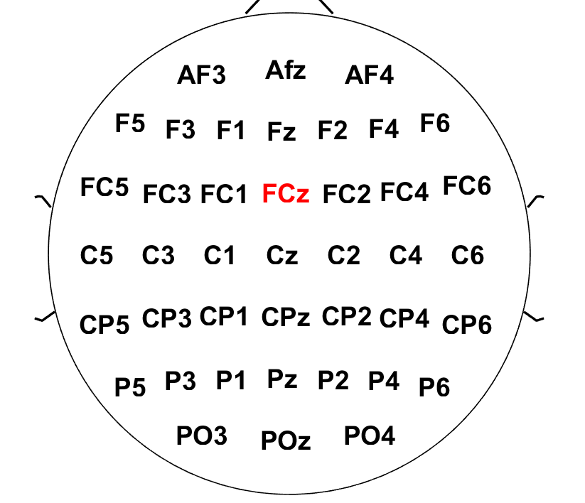
Error‐ Related Potentials (ErrPs) are slow cortical potentials seen in the EEG signal of human subjects that are elicited by an unexpected (erroneous) outcome. For example, within the context of human-machine interaction, such signals are observed when the machine takes an unexpected action [9, 4, 5]. In this section, we illustrate the efficacy of the proposed DMD algorithms on EEG recordings taken from Monitoring Error-Related Potentials database [4, 5]. These EEG recordings were collected from six subjects while they were observing the movement of a cursor between two labeled targets on a screen. The subjects had no control on the motion of the cursor. However, they had a priori knowledge about the intended directions of movement. The cursor movements were set to elicit ErrPs by generating two types of events, namely, correct events and erroneous events. The correct events correspond to the cursor movement in the intended direction, while the erroneous events correspond to the cursor movement in any unintended direction. EEG signals were recorded at sampling rate of 512512512 Hz, using Biosemi ActiveTwo system with 646464 electrodes distributed according to the standard 10/20102010/20 international system as it is shown in Figure 1.
Refer to caption
Fig. 1: Topographical view for EEG channels with the channel FCz, where the ErrPs can be characterized, marked in red bold font

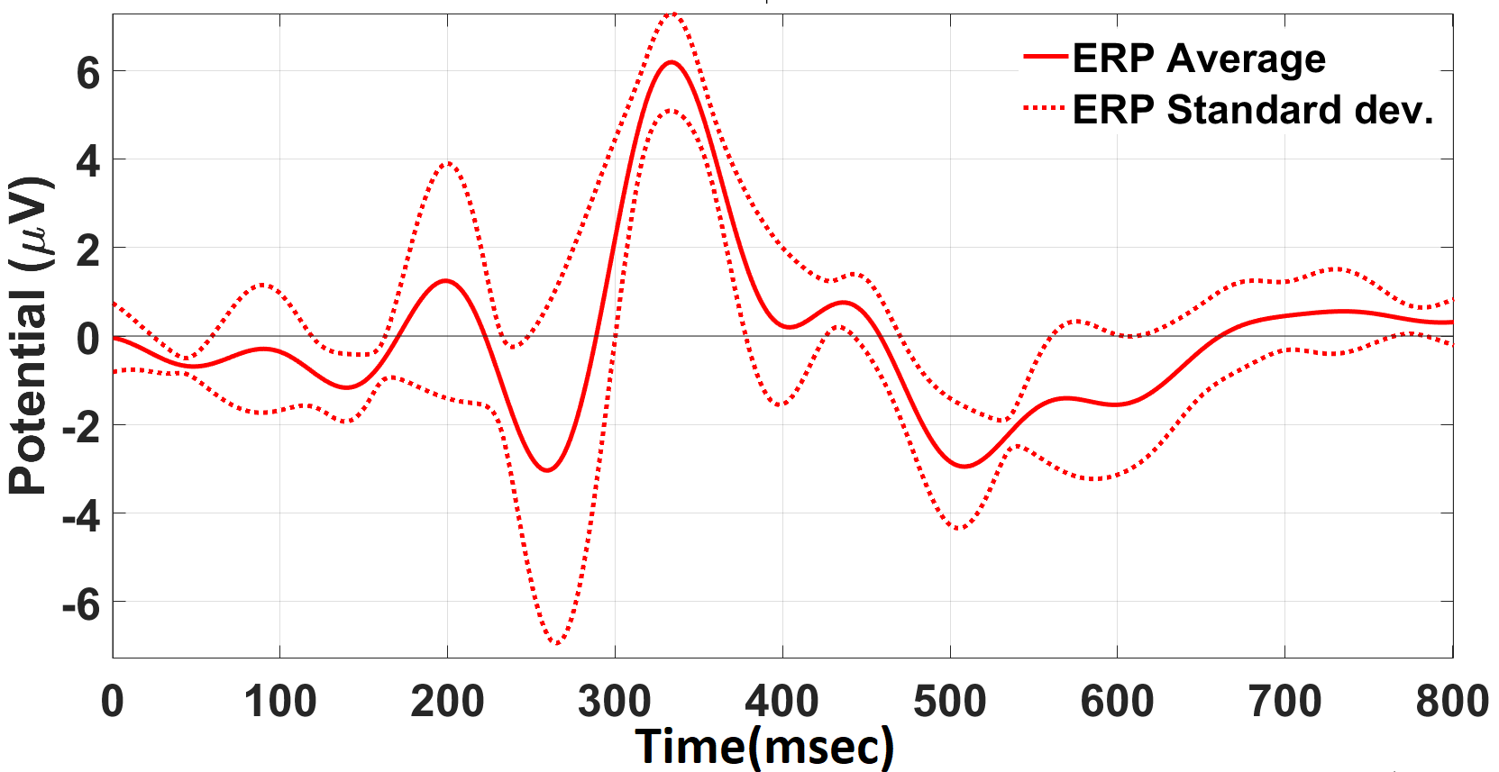
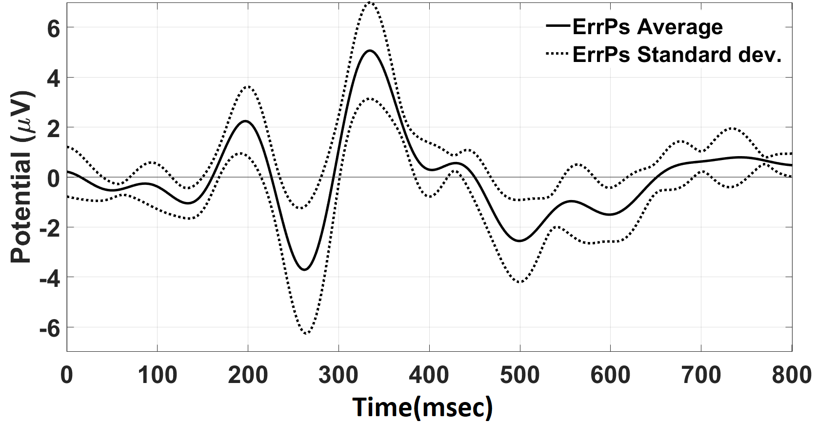
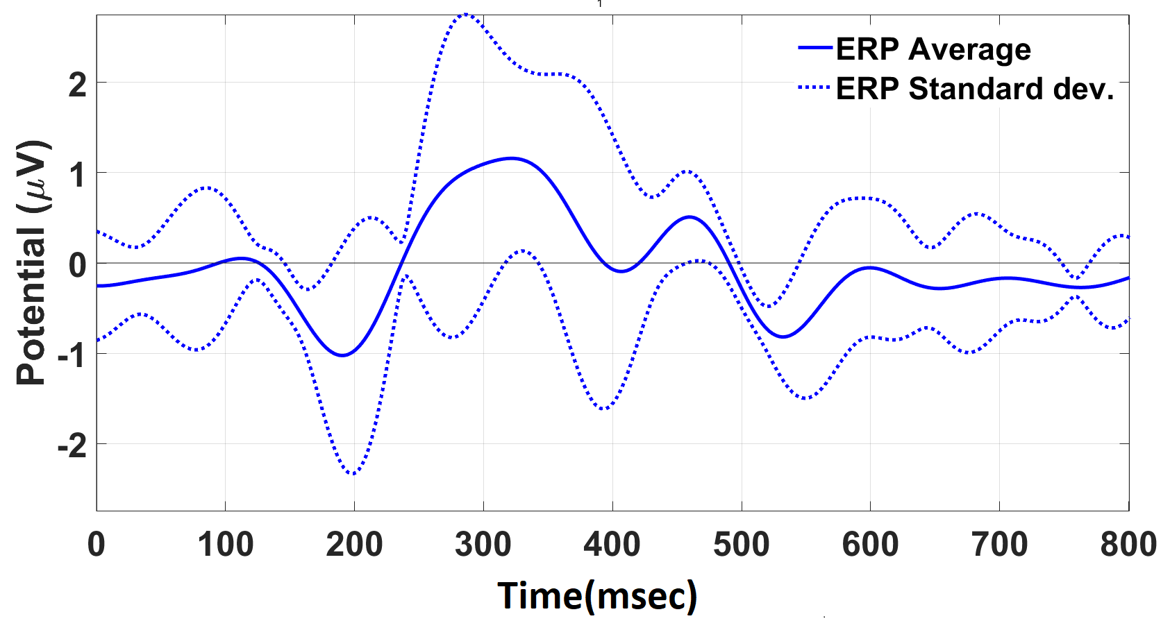
A two step standard EEG preprocessing for ErrPs which consists of Common Average Reference (CAR) filtering, and then (110)110(1-10) Hz Band Pass (BP) filtering is performed on the data. Segments of EEG signals, from all the participants, corresponding to the correct and erroneous events were extracted into two separate groups. Then, the segments within each group were averaged to obtain a signal each for the correct and erroneous events. Finally, the ErrPs are calculated by subtracting the signal for correct event from the signal for the erroneous event. Figure 2 shows the ERP signals and topographical views corresponding to the correct and erroneous events, and the calculated ErrPs. EEGLAB was used for the processing of EEG signals and generating the topographical views for the related brain activities [8]. Note that for consistency with the literature, we investigate the averaged ERP signal. However, the confidence regions around the averaged signal shown in Figure 2 reveal that despite the variability in these signals, the key features are also seen in the signal associated with a single event. Thus, the following analysis can be performed on a single subject real time data as well.

As reported in [4, 5], the ErrPs are characterized by a sequence of three peaks/troughs after the onset of the event in the EEG signal measured at channel FCz (see Figure 1). A sample ErrP is shown in Figure 2c where the first small positive peak is observed at 200 ms, followed by a negative trough at 260 ms, and finally a larger positive peak at 330 ms.

Two observations can be made by comparing the temporal behavior and the topographical views during the correct and erroneous events in Figures 2a and 2b, respectively. First, the ERP signal during the correct event tends to have broader peaks in comparison with the ERP signal during erroneous events, which indicates that it has slower dynamics, i.e., has smaller growth or decay rates. Second, by comparing the topographical views during the three characterizing peaks at FCz channel, it can be noticed that the ERP peaks during erroneous events have higher amplitudes than the peaks during correct events in both negative and positive directions. Note that the colormap bar values are different for the topographical views for the correct ERP, the erroneous ERP, and the ErrP in Figure 2.
Refer to caption
Refer to caption
(a) EEG pattern during correct event
Refer to caption
Refer to caption
(b) EEG pattern during erroneous event
Refer to caption
Refer to caption
(c) Differential EEG pattern
Fig. 2: The average response to an event at t=0𝑡0t=0: the mean ERP (confidence level = 95%percent9595\%) at the FCz channel (left panel) and the topographical view for brain activity across all channels (right panel). The top and middle panels show the patterns during the correct event and the erroneous event, respectively. The bottom panel shows that ErrP obtained by subtracting the signal associated with the correct event from that of the erroneous event. The topographical views are shown at the three characterizing peaks that occur at 200200200 msec, 260260260 msec, and 360360360 msec, respectively.

As shown in Figure 2, the EEG patterns show coherent activities within the brain suggesting the possibility of a low-dimensional dynamics underlying this high dimensional data. Furthermore, these patterns change significantly with time and can possibly be better explained using a time-varying underlying model. To investigate these hypotheses, we apply the incremental DMD algorithms to the EEG recordings corresponding to correct and erroneous events. The weighted incremental DMD algorithm is applied with discounting factors ρ={0.1,0.2,0.4,0.8}𝜌0.10.20.40.8\rho=\left\{0.1,0.2,0.4,0.8\right\}, and the windowed incremental DMD algorithm with a time-window of width w=512𝑤512w=512 samples. All singular values greater than σthr={0.01,0.001}subscript𝜎thr0.010.001\sigma_{\text{thr}}=\{0.01,0.001\} are used for computing the reduced order DMD operator. An initial window of 512512512 samples before the event occurrence is used to initialized the DMD models for both algorithms.

We compare the proposed algorithms with the online DMD approach proposed in [35]. To this end, we use the same parameters (discounting factor and width of time-window) in the online DMD algorithms as the incremental DMD algorithms. Recall that the online DMD algorithms rely on the Sherman-Morrison identity to compute the DMD operator and do not have access to the (time-varying) singular values of the data matrix and hence, the reduction of the DMD operator to leading singular vectors does not apply to online DMD algorithms.

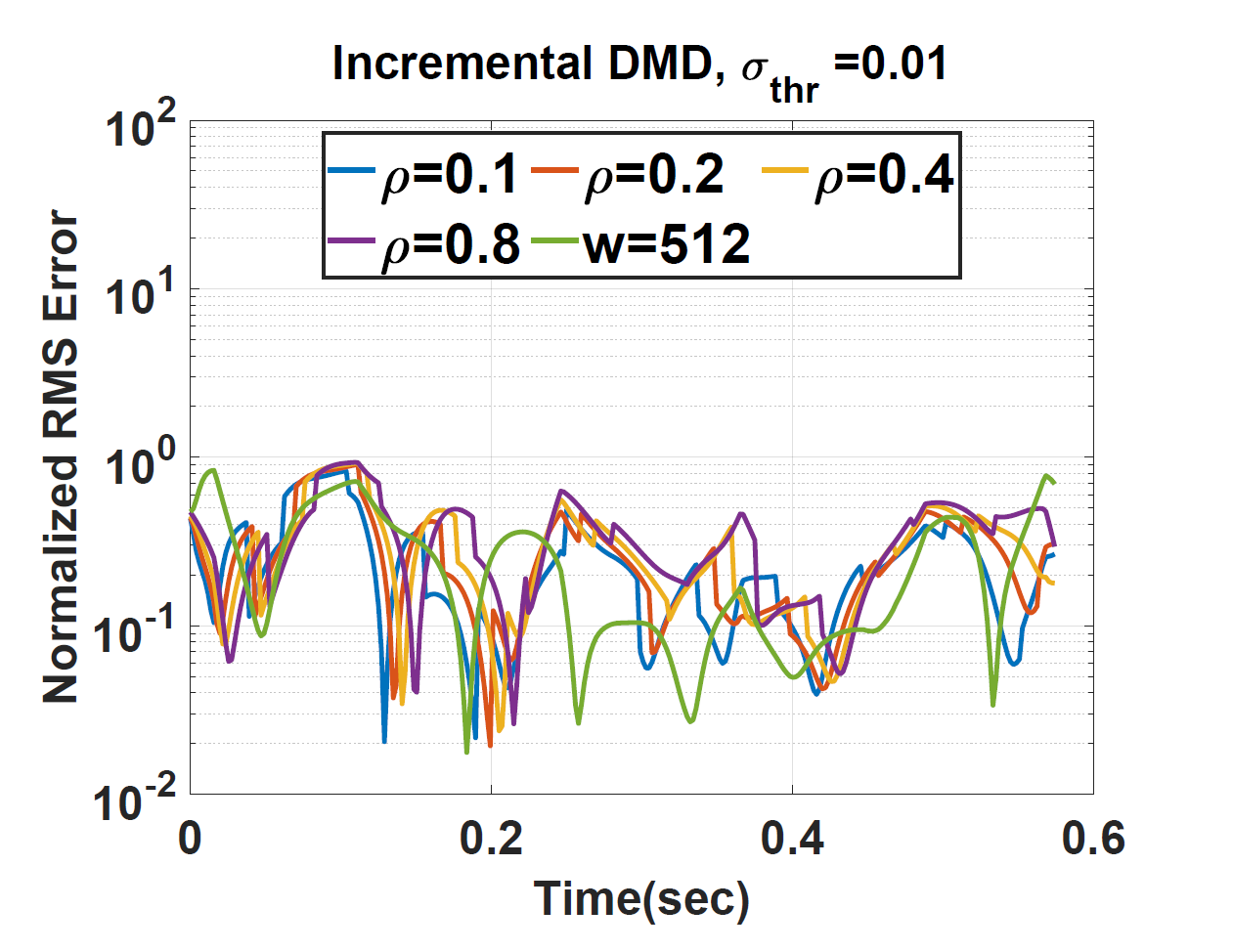
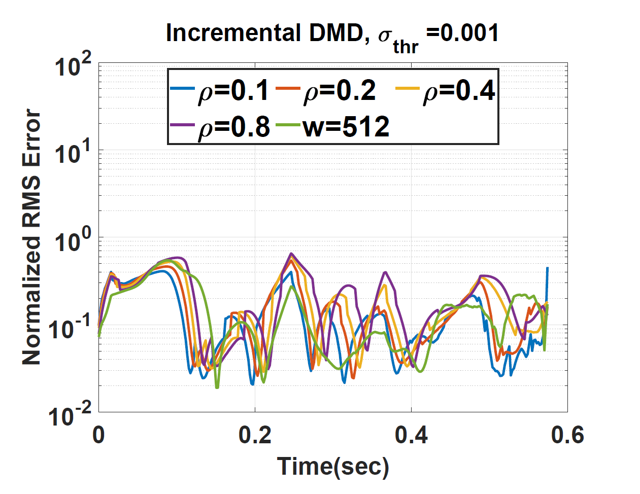
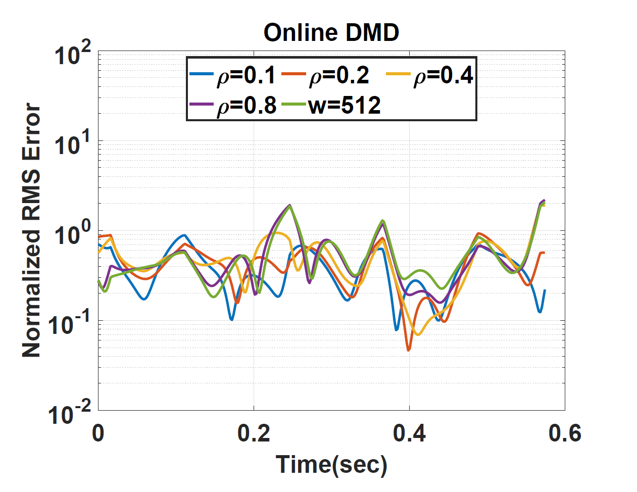
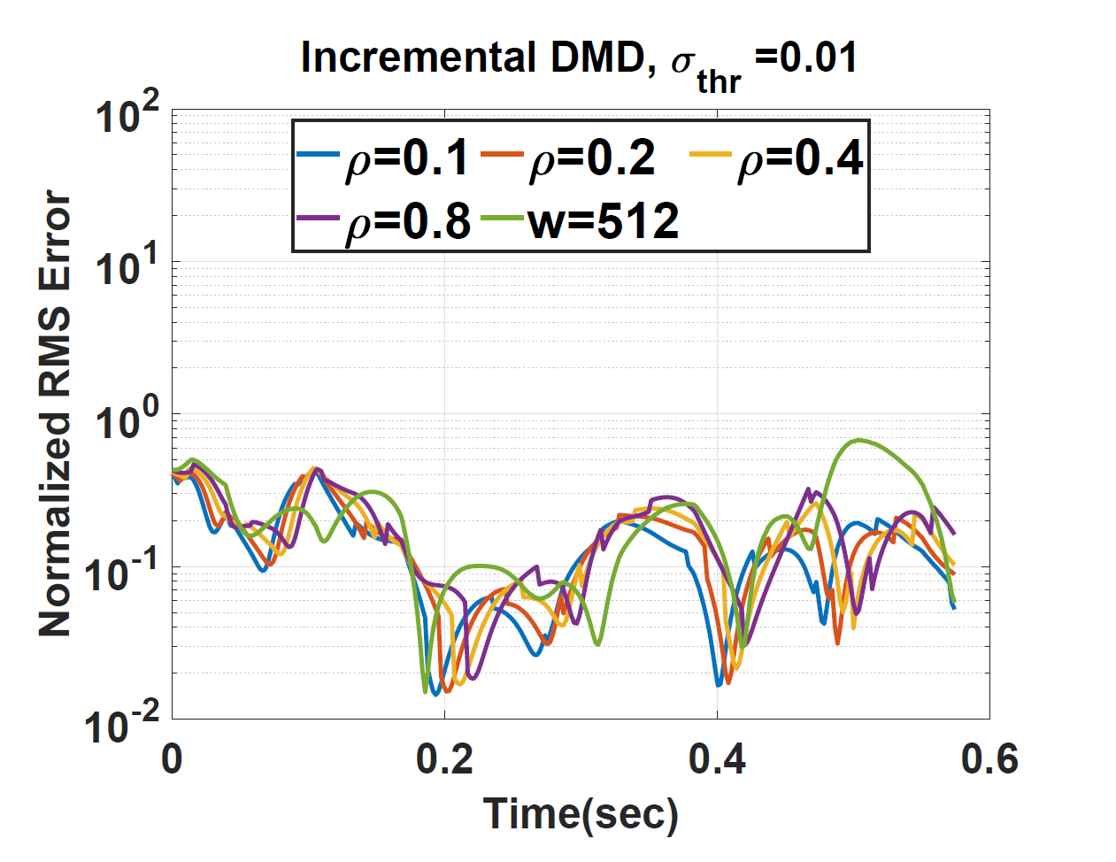
In order to compute the time-varying DMD operator, we first compute a standard DMD operator using EEG data from a one-second window (512512512 samples) just before the correct or erroneous event. Subsequently, the EEG measurements are streamed with a rate of 111 sample/iterationsampleiteration\text{sample}/\text{iteration} to update the initial DMD operator. At each iteration, both weighted and windowed versions of the incremental DMD and online DMD algorithms are used to predict 646464 future samples of the EEG signal at channel FCz. We compare the performance of these algorithms using normalized Root Mean Square (RMS) prediction error, denoted as enrms(k)subscript𝑒nrms𝑘{e}_{\text{nrms}}(k) at each tk{0,,0.6}subscript𝑡𝑘00.6t_{k}\in\{0,\cdots,0.6\} using the following formula:

enrms(k)=164i=k+1k+64(𝐲^i𝐲i)2𝐲¯k𝐲¯k,subscript𝑒nrms𝑘164superscriptsubscript𝑖𝑘1𝑘64superscriptsubscript^𝐲𝑖subscript𝐲𝑖2subscript¯𝐲𝑘subscript¯𝐲𝑘{e}_{\text{nrms}}(k)=\frac{\sqrt{\frac{1}{64}\sum_{i=k+1}^{k+64}(\hat{\mathbf{y}}_{i}-\mathbf{y}_{i})^{2}}}{\overline{\mathbf{y}}_{k}-\underline{\mathbf{y}}_{k}}, (40)

where 𝐲^isubscript^𝐲𝑖\hat{\mathbf{y}}_{i} and 𝐲isubscript𝐲𝑖\mathbf{y}_{i} are the estimated and recorded values, respectively, 𝐲¯k=maxk+1ik+64𝐲isubscript¯𝐲𝑘subscript𝑘1𝑖𝑘64subscript𝐲𝑖\overline{\mathbf{y}}_{k}=\max\limits_{k+1\leq i\leq k+64}\mathbf{y}_{i}, and 𝐲¯k=mink+1ik+64𝐲isubscript¯𝐲𝑘subscript𝑘1𝑖𝑘64subscript𝐲𝑖\underline{\mathbf{y}}_{k}=\min\limits_{k+1\leq i\leq k+64}\mathbf{y}_{i}.

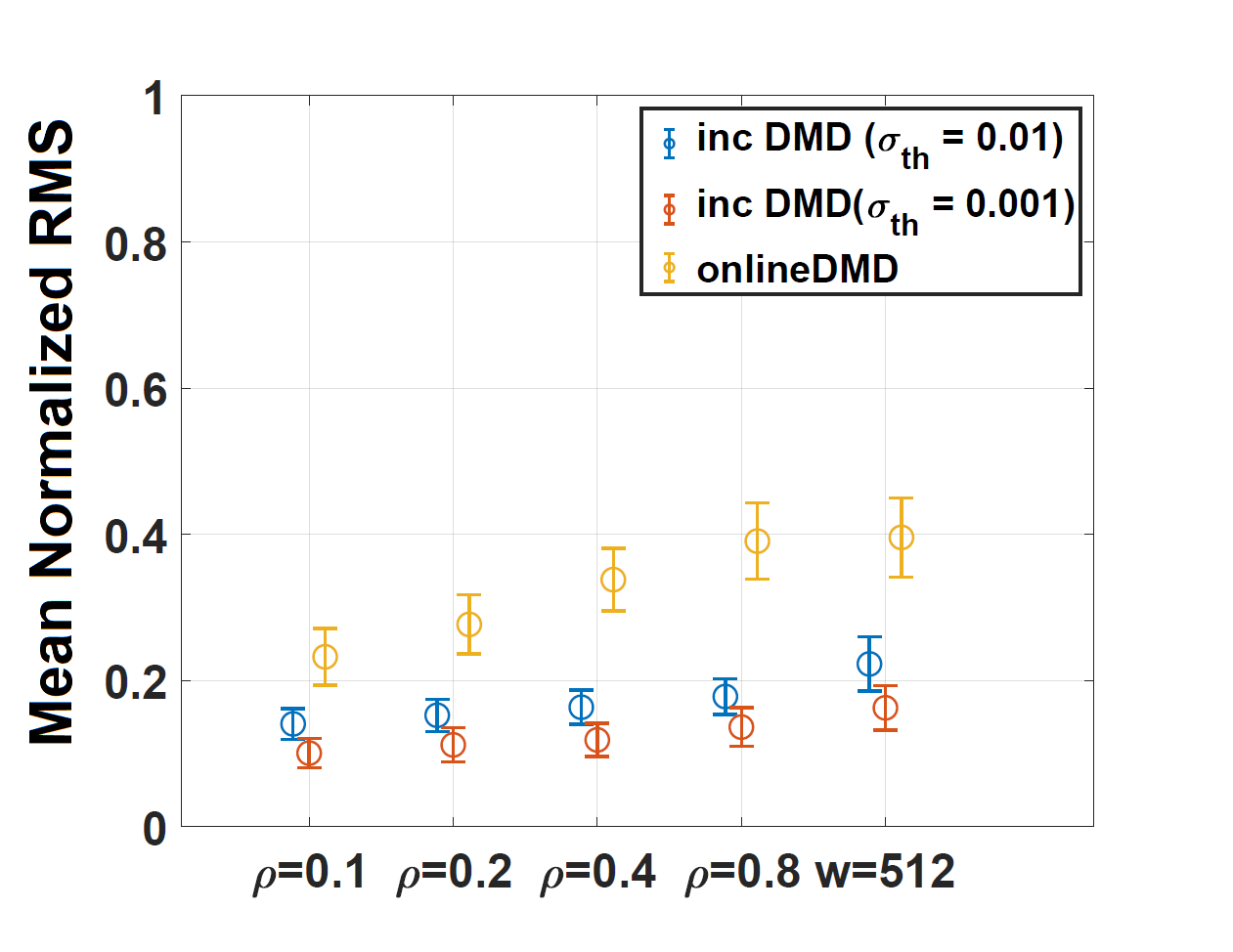
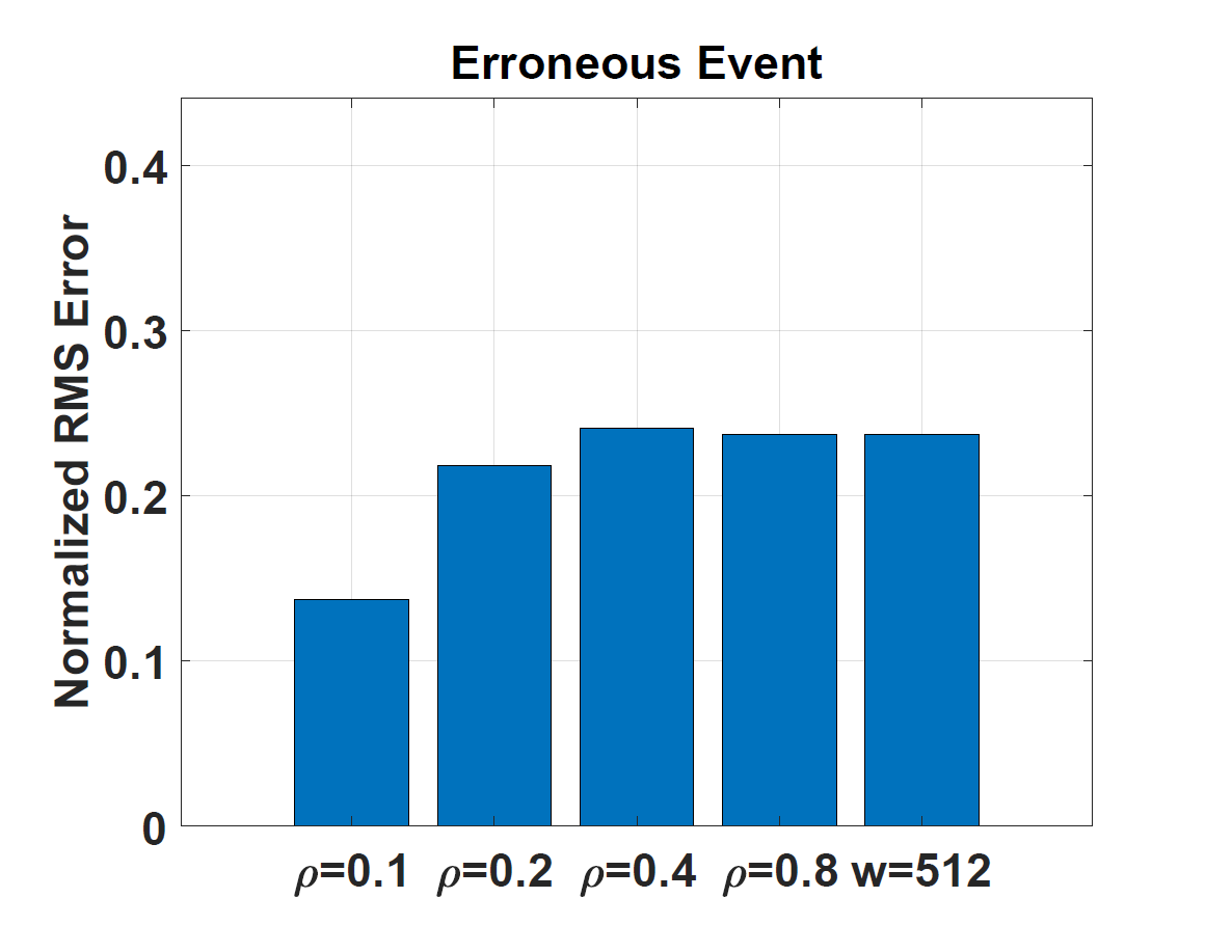
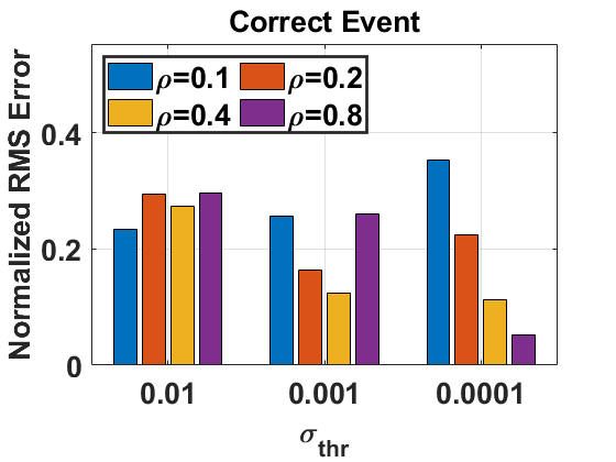
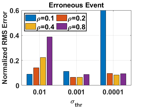
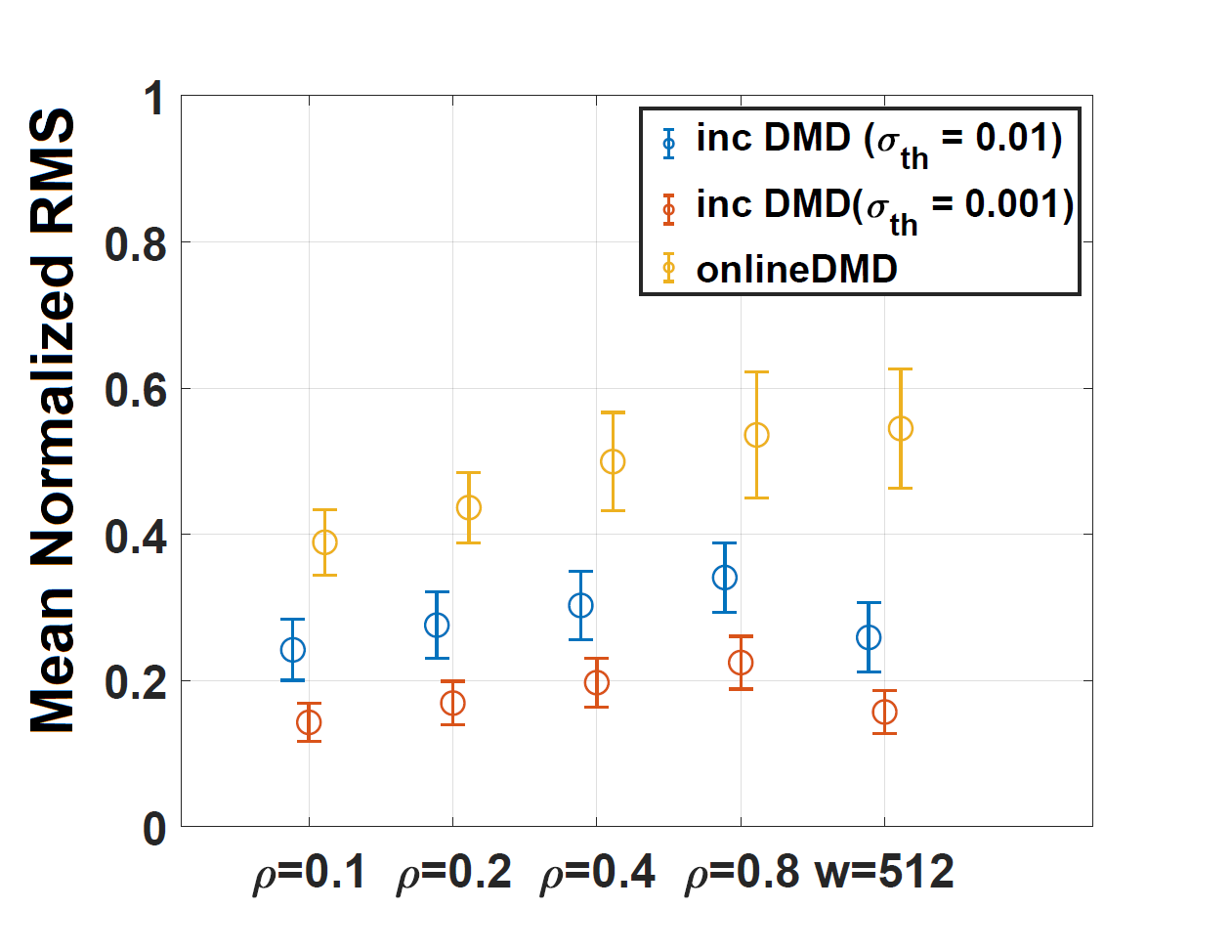
Figure 3 shows the mean of the normalized RMS prediction error computed over all iterations as well as the associated 95% confidence sets for weighted and windowed incremental DMD algorithms and different choices of parameters. The performance of the incremental DMD does not appear to vary much with the weighting factor and the two choices of the threshold on singular values. The performance of the windowed incremental DMD algorithm is similar to the weighted incremental DMD. However, incremental DMD algorithms seem to outperform online DMD algorithms. This suggests that having a small threshold σthrsubscript𝜎thr\sigma_{\textup{thr}} is more beneficial than having no threshold as in the case of online DMD algorithms. Figure 13 in Appendix E presents the evolution of the normalized RMS prediction error for each event.
Refer to caption
(a) Correct Event
Refer to caption
(b) Erroneous Event
Fig. 3: The mean of the normalized RMS prediction error computed over all iterations as well as the associated 95% confidence sets for (a) correct events and (b) erroneous events.

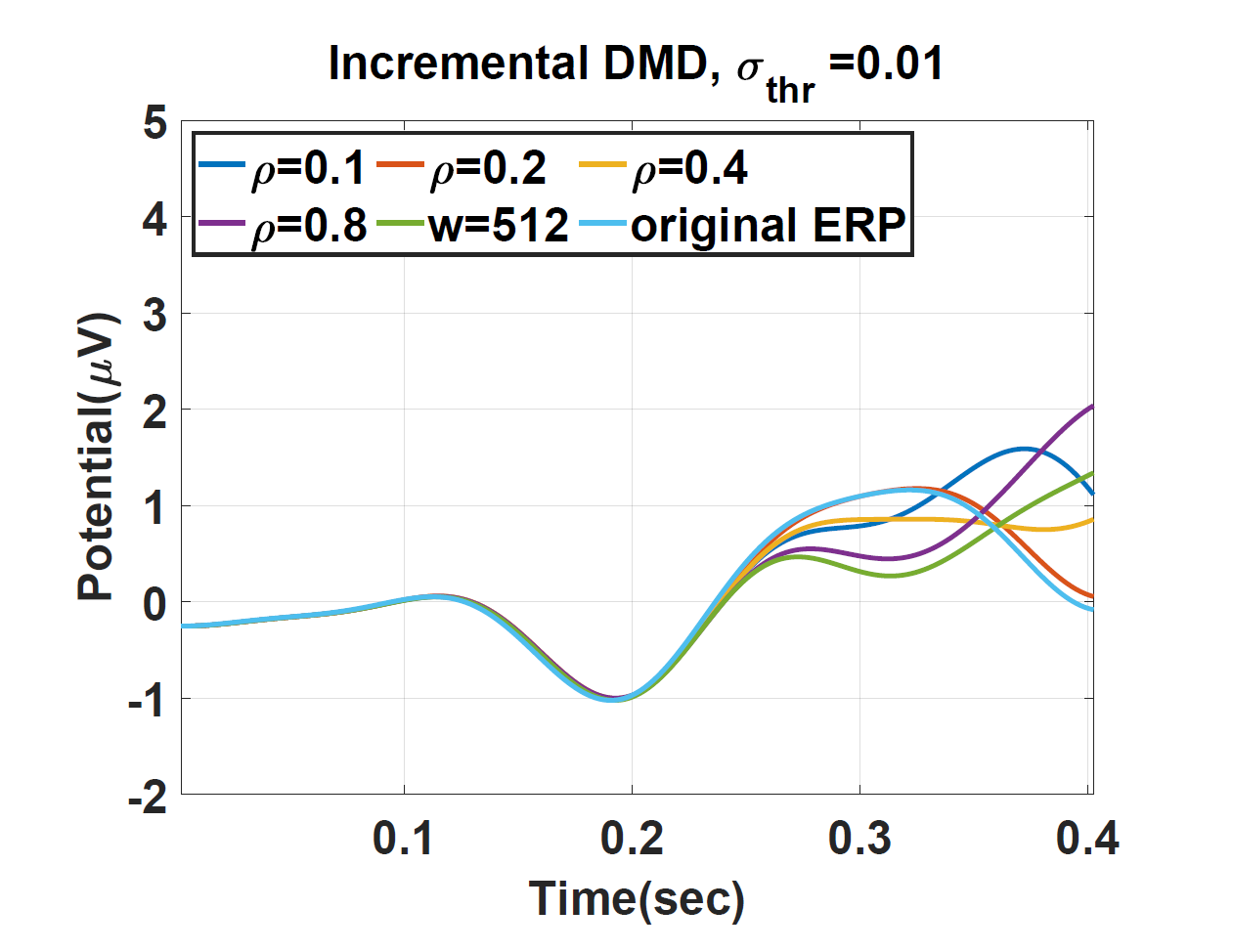
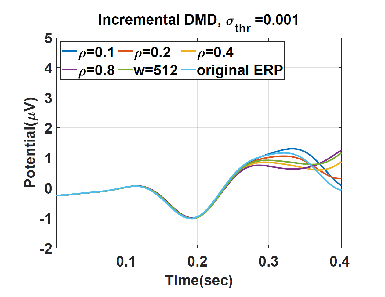
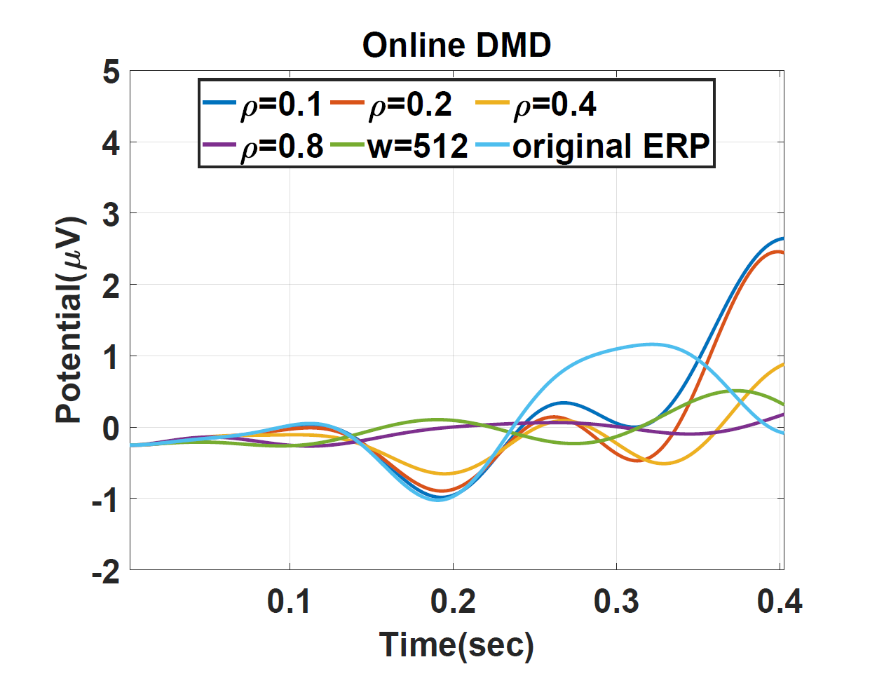
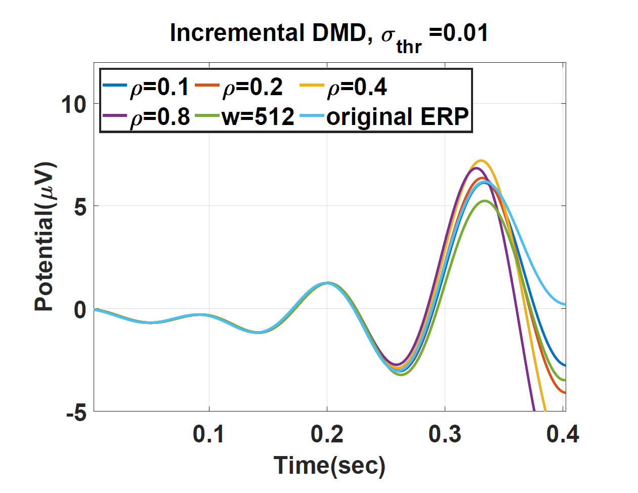
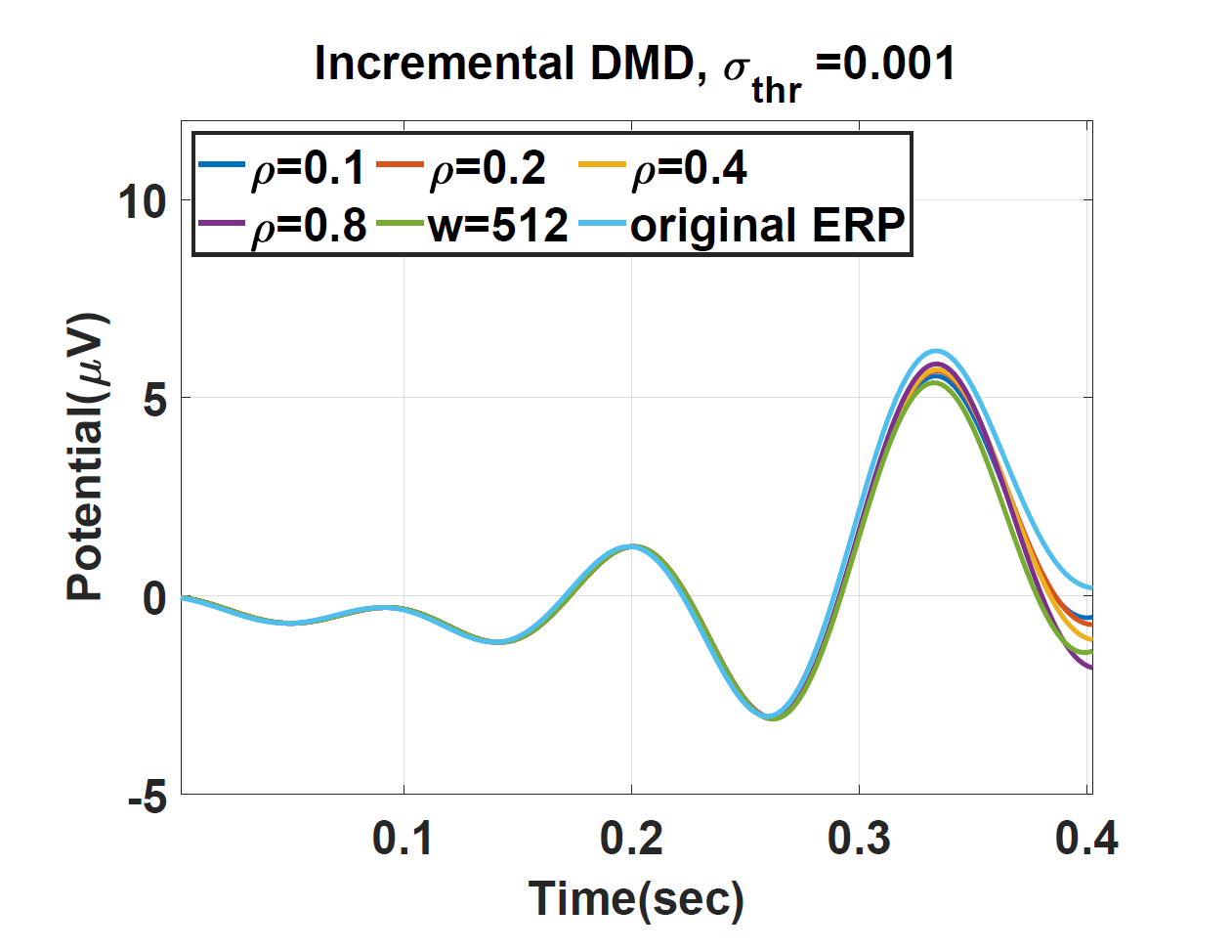
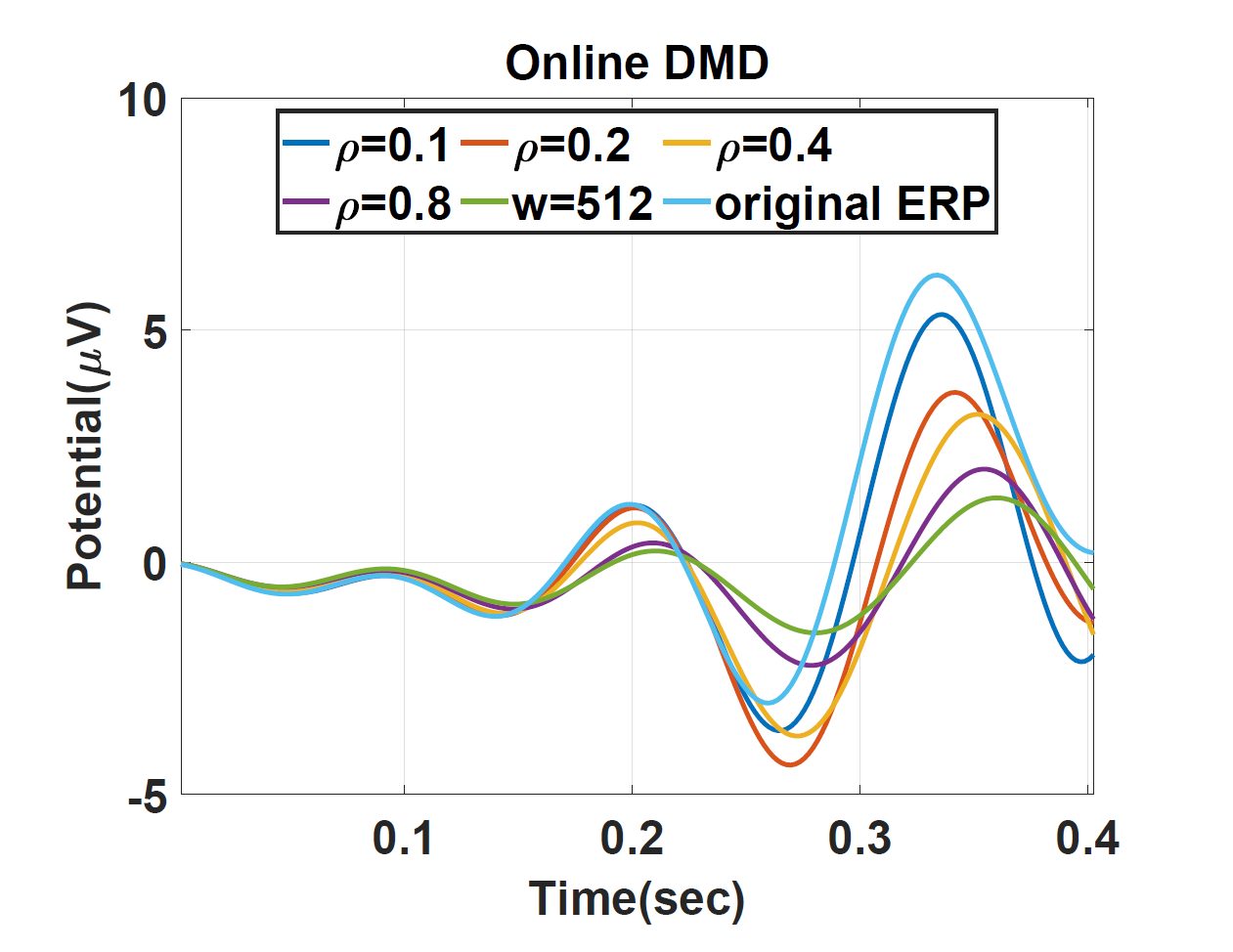
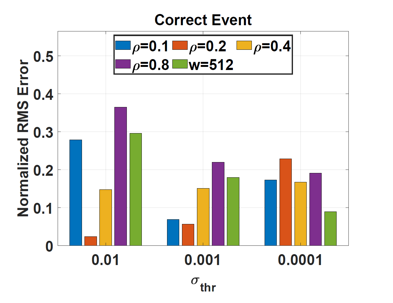
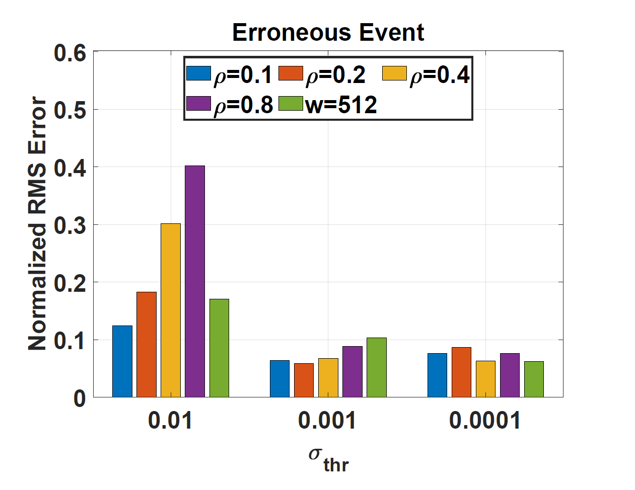
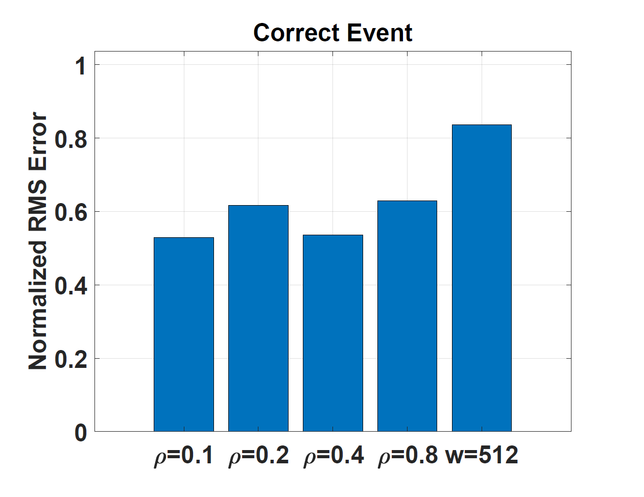
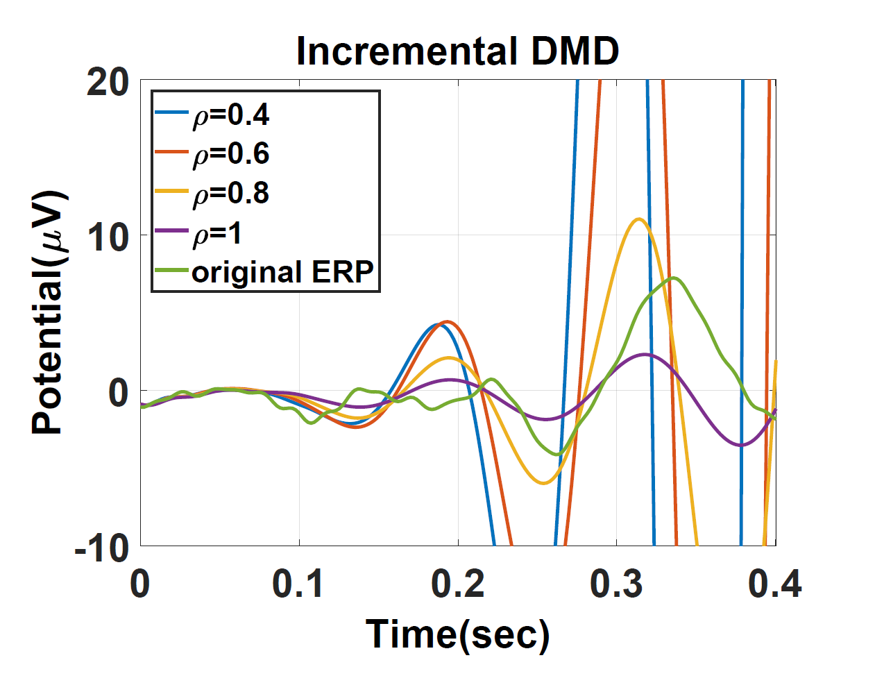
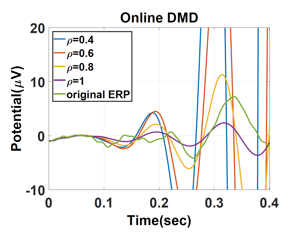
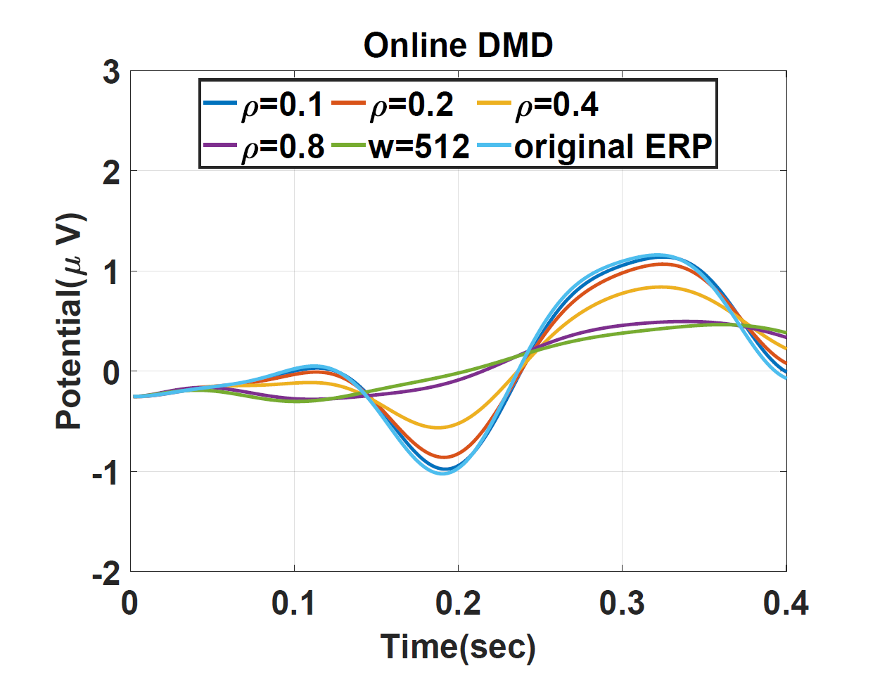
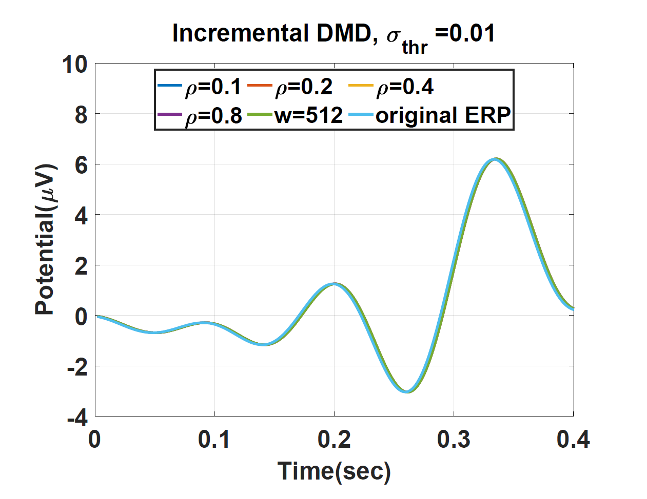
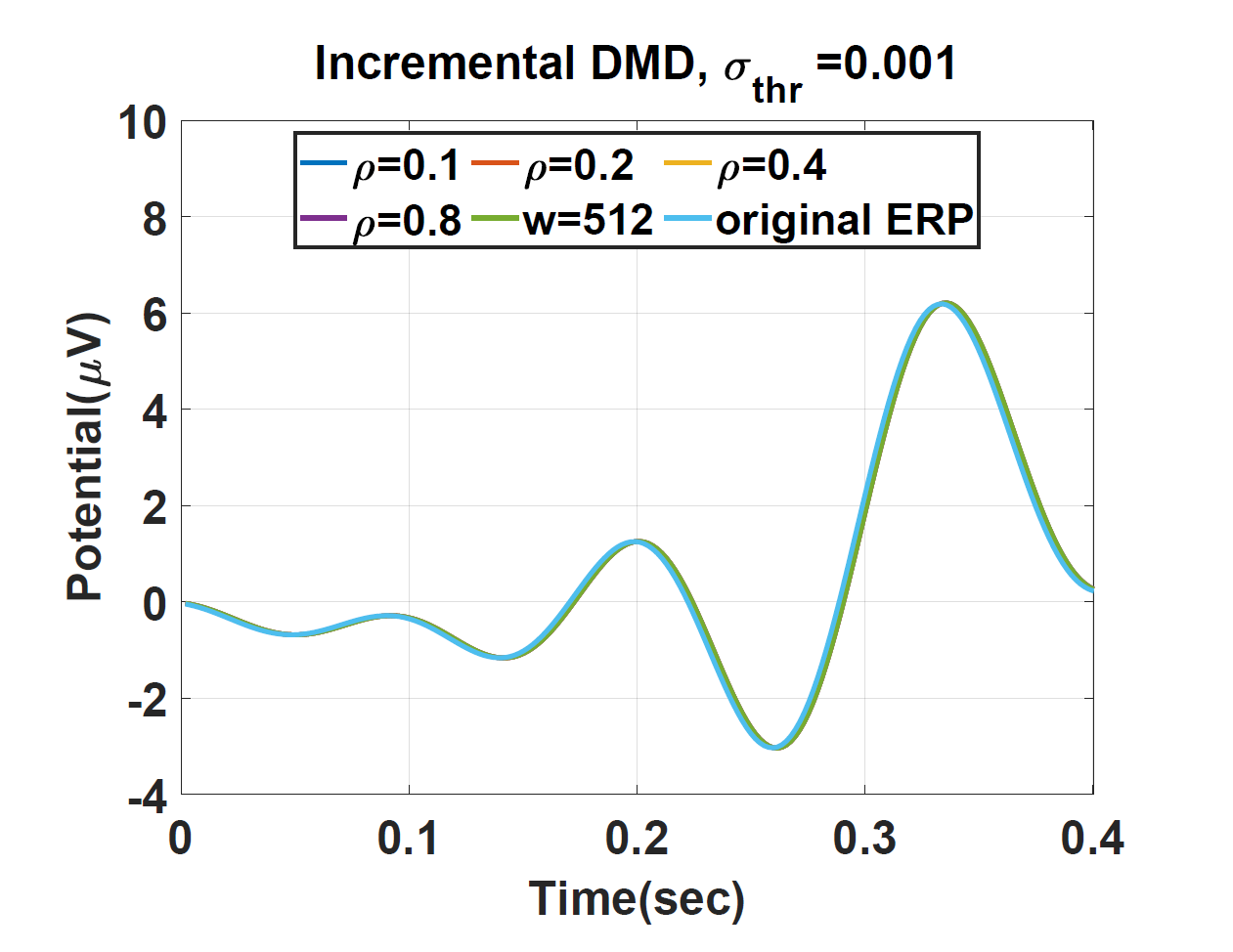
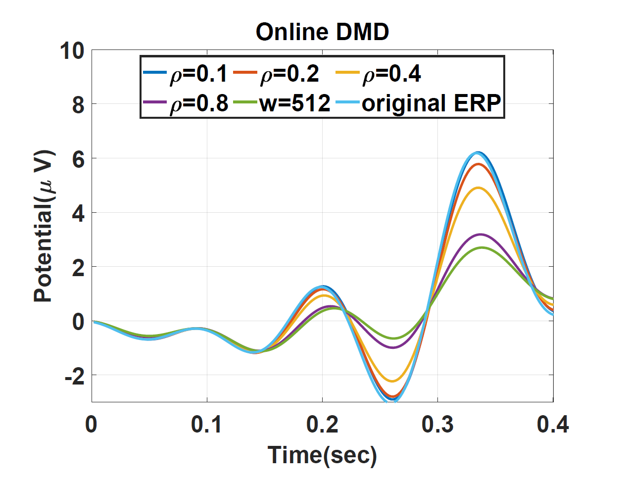
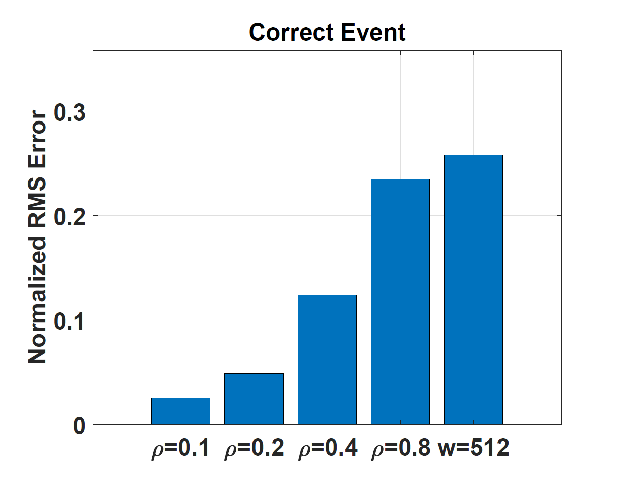
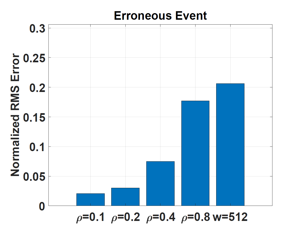
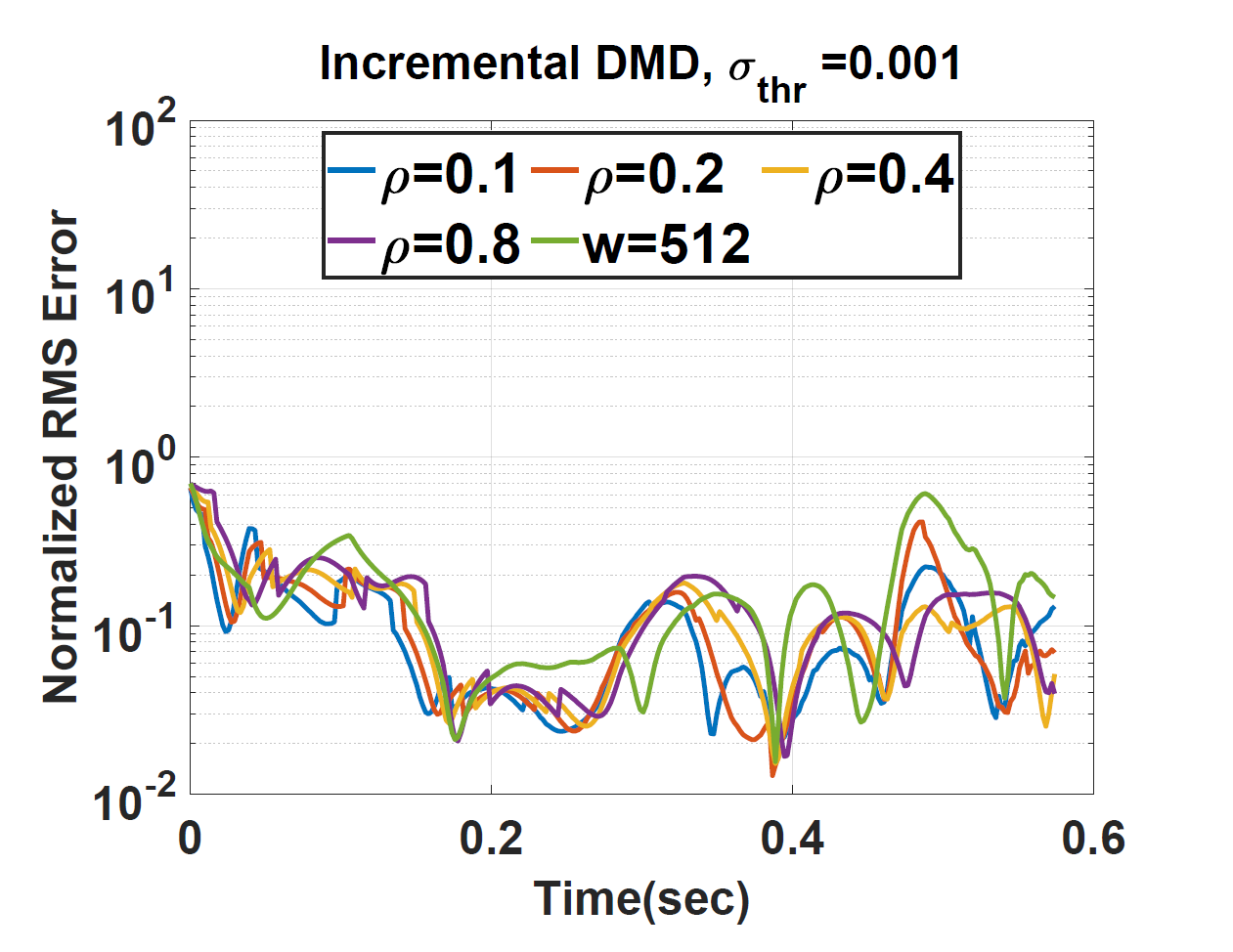
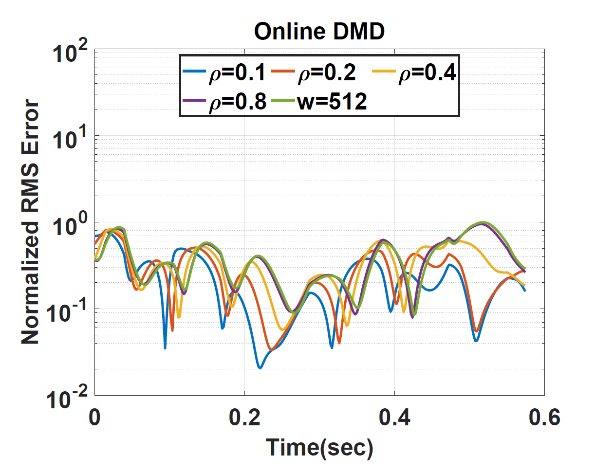
In order to gain further insight into the influence of different thresholds σthrsubscript𝜎thr\sigma_{\text{thr}} and weighting factors ρ𝜌\rho, we investigate how accurately the incremental DMD predicts the signature ERPs at channel FCz. To this end, we updated the initial DMD operator using incremental DMD algorithms until the first peak at 200 msec. We then used the updated lower-dimensional DMD operator to predict the future ERP until the third peak at 330 msec. The predicted signal and the associated normalized RMS are shown in Figures 4 and 5, respectively. For the erroneous event, the predicted signal from incremental DMD algorithms capture the trend of the original signal, while for the correct event, most incremental DMD algorithms fail to capture the final dip in the original signal. The only exception is the windowed incremental DMD with σthr=0.001subscript𝜎thr0.001\sigma_{\textup{thr}}=0.001. For σthr=0.01subscript𝜎thr0.01\sigma_{\textup{thr}}=0.01, the number of DMD modes used by the incremental DMD algorithms range from 26 to 31 for correct events and 28 to 32 for erroneous events. Similarly, for σthr=0.001subscript𝜎thr0.001\sigma_{\textup{thr}}=0.001, the number of DMD modes used by the incremental DMD algorithms range from 26 to 31 for correct events and 28 to 33 for erroneous events. In comparison, the predicted signal from the online DMD algorithms performs poorly. The key reason for this poor performance, is that the data matrix obtained after prepossessing is not full rank even if all the measurements are included. Thus, the Sherman-Morrison update cannot be applied in the standard form. Recall that the online DMD algorithm starts by initializing the DMD operator 𝐀ksubscript𝐀𝑘\mathbf{A}_{k} and the inverse of covariance matrix 𝐏k=(𝐗k𝐗kT)1subscript𝐏𝑘superscriptsubscript𝐗𝑘superscriptsubscript𝐗𝑘T1\mathbf{P}_{k}=\left(\mathbf{X}_{k}\mathbf{X}_{k}^{\text{T}}\right)^{-1}. For initialization of online DMD algorithms, we adopted the suggestion in [35]: in the event that 𝐗k𝐗kTsubscript𝐗𝑘superscriptsubscript𝐗𝑘T\mathbf{X}_{k}\mathbf{X}_{k}^{\text{T}} is not full rank, 𝐀ksubscript𝐀𝑘\mathbf{A}_{k} can be initialized by an n×n𝑛𝑛n\times n zero matrix, and 𝐏ksubscript𝐏𝑘\mathbf{P}_{k} can be initialized by 𝐏init=αIsubscript𝐏init𝛼I\mathbf{P}_{\text{init}}=\alpha\text{I} where α𝛼\alpha is a large positive scalar.

Refer to caption
Refer to caption
Refer to caption
(a) Correct event
Refer to caption
Refer to caption
Refer to caption
(b) Erroneous event
Fig. 4: Predicted ERP signal at channel FCz using incremental DMD with σthr=0.01subscript𝜎thr0.01\sigma_{\text{thr}}=0.01 (left panel), incremental DMD with σthr=0.001subscript𝜎thr0.001\sigma_{\text{thr}}=0.001 (middle panel), and online DMD (right panel) for (a) correct event, and (b) erroneous event.
Refer to caption
Refer to caption
(a) Incremental DMD
Refer to caption
Refer to caption
(b) Online DMD
Fig. 5: Normalized RMS error for the predicted ERP signal at channel FCz for correct events (left panel) and erroneous events (right panel), using (a) incremental DMD, and (b) online DMD.

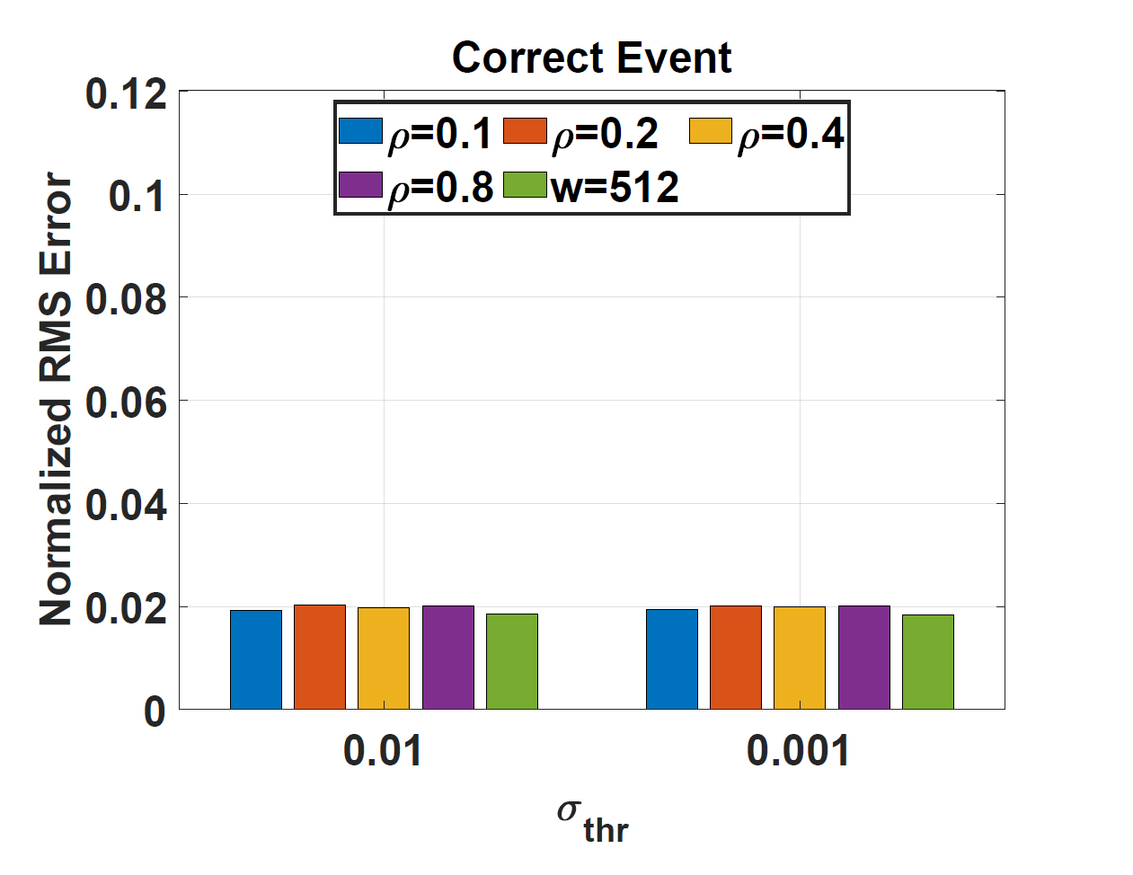
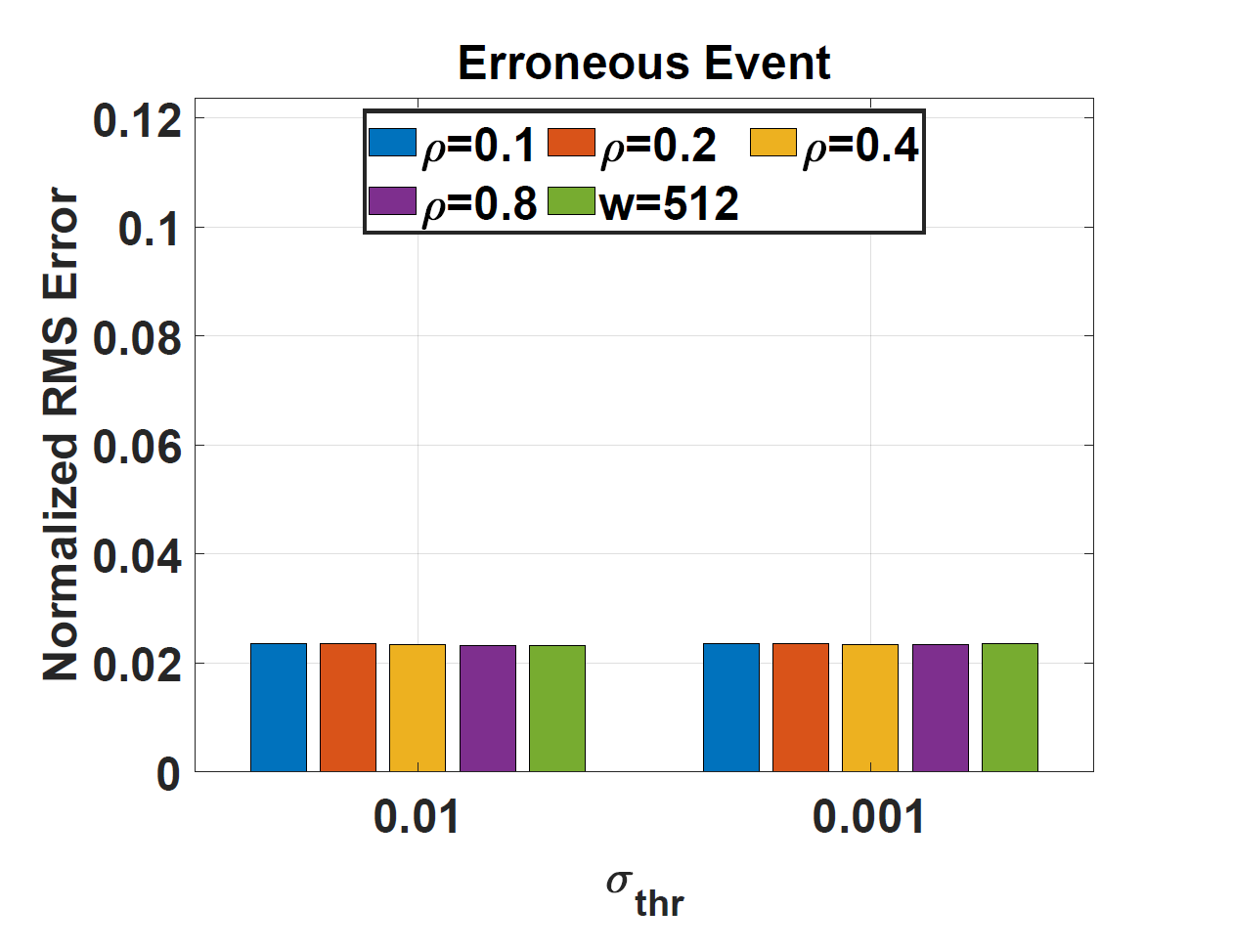
During the correct events, there appears to be an interplay between the threshold σthrsubscript𝜎thr\sigma_{\text{thr}} and weighting factor ρ𝜌\rho. As shown in Figure 5 for correct events, the normalized RMS decreases with decreasing the weighting factor until ρ=0.2𝜌0.2\rho=0.2 and increases with further decrease in ρ𝜌\rho. For ρ=0.2𝜌0.2\rho=0.2, the higher dimension of the reduced system (σthr=0.001subscript𝜎thr0.001\sigma_{\textup{thr}}=0.001) leads to higher prediction error compared with the lower dimension reduced system (σthr=0.01subscript𝜎thr0.01\sigma_{\textup{thr}}=0.01). This suggests that for a weighting factor that leads to the smallest prediction error, including too many modes is not beneficial for prediction performance, since it leads to over-fitting. A similar interplay is not seen for the erroneous event in Figure 5. However, if we choose a smaller initial window to initialize the DMD model, we observe similar effects as shown in Figure 14 in Appendix F. Similar effects are observed for the windowed DMD as shown in Figure 15 in Appendix F.

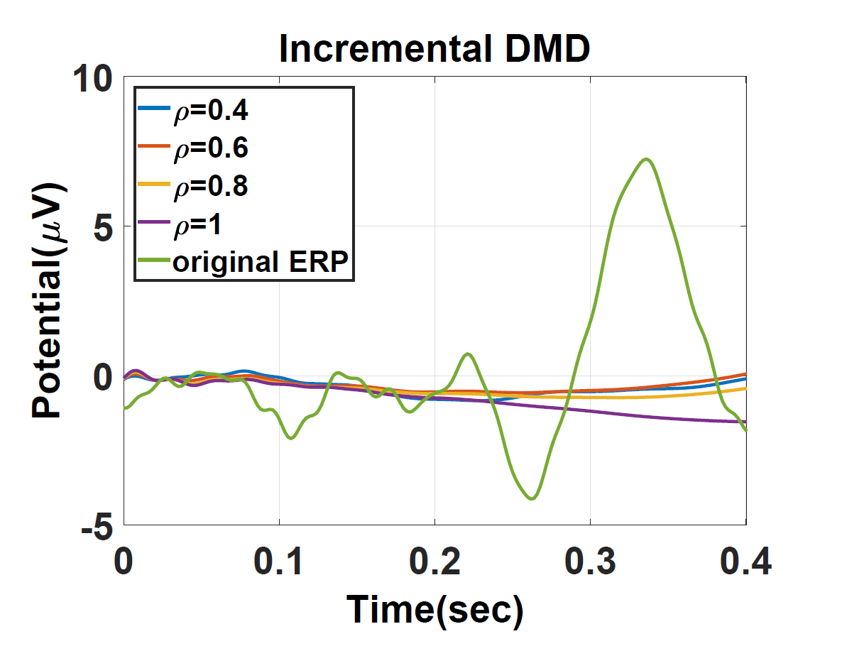
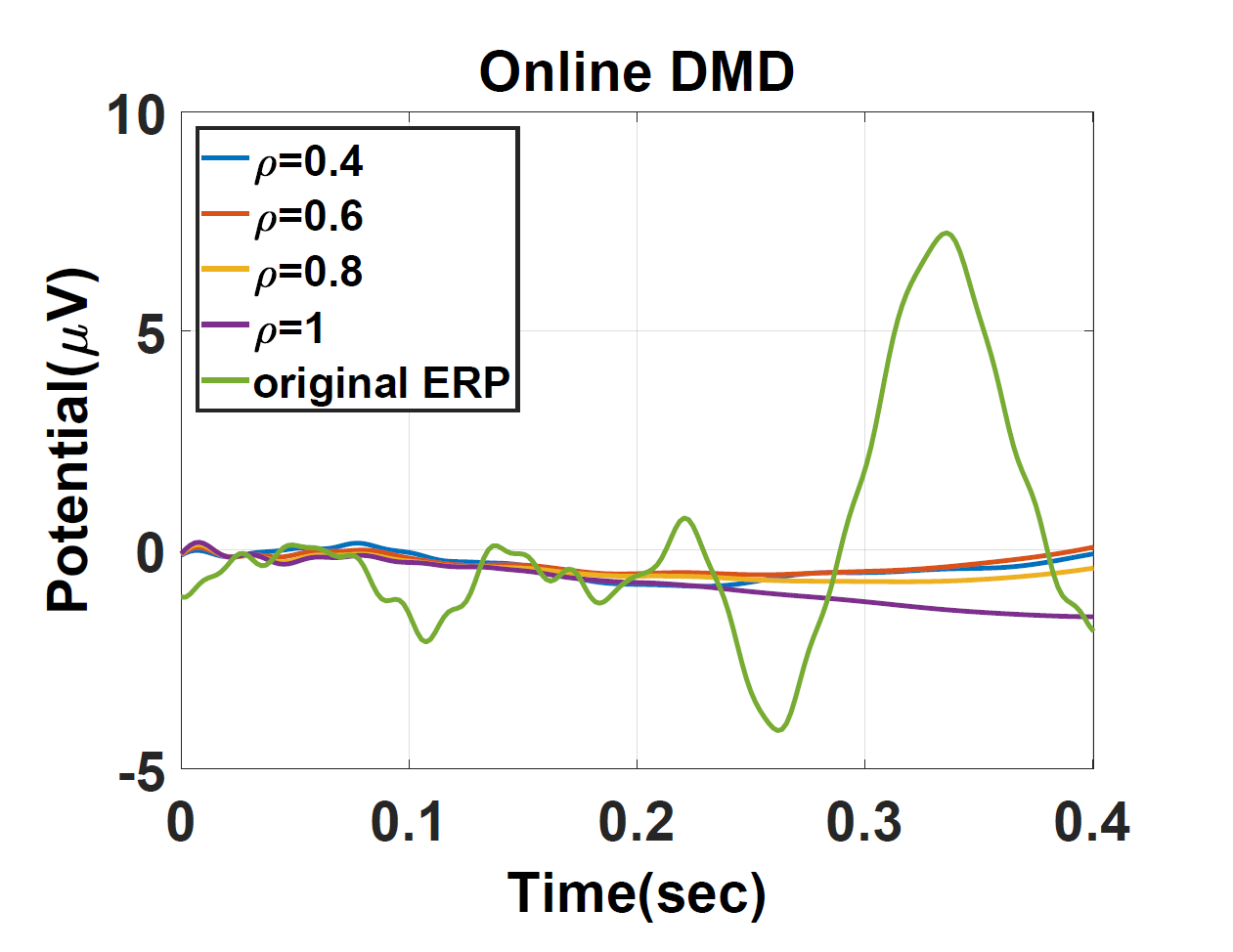
To further compare the online DMD with the incremental DMD, we took the raw EEG data, i.e., data without any preprocessing (CAR and BP filtering). In this case, the data matrix is well-conditioned and the Sherman-Morrison identity is well defined. The performance of online DMD and the incremental DMD in terms of predicting future signal is shown in Figure 6. In this case, both incremental and online DMD algorithms have similar poor performance. This suggests that the difference in the performance of these algorithms is primarily due to ill-conditioned dataset. This also highlights the utility of applying appropriate band-pass filtering to the raw EEG data. Without such filtering, the key activities seem to be lost in the background noise resulting in a poor prediction performance.
Refer to caption
Refer to caption
(a) correct events
Refer to caption
Refer to caption
(b) erroneous events
Fig. 6: The predicted ERP signal at channel FCz based on well conditioned EEG datasets using incremental DMD model (left panel) and online DMD model (right panel) during (a) correct events and (b) erroneous events.

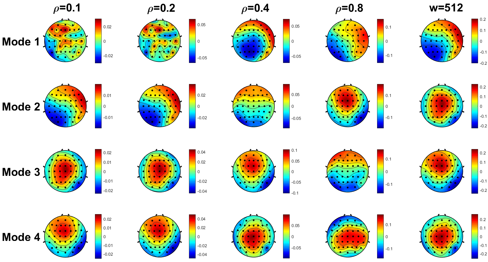
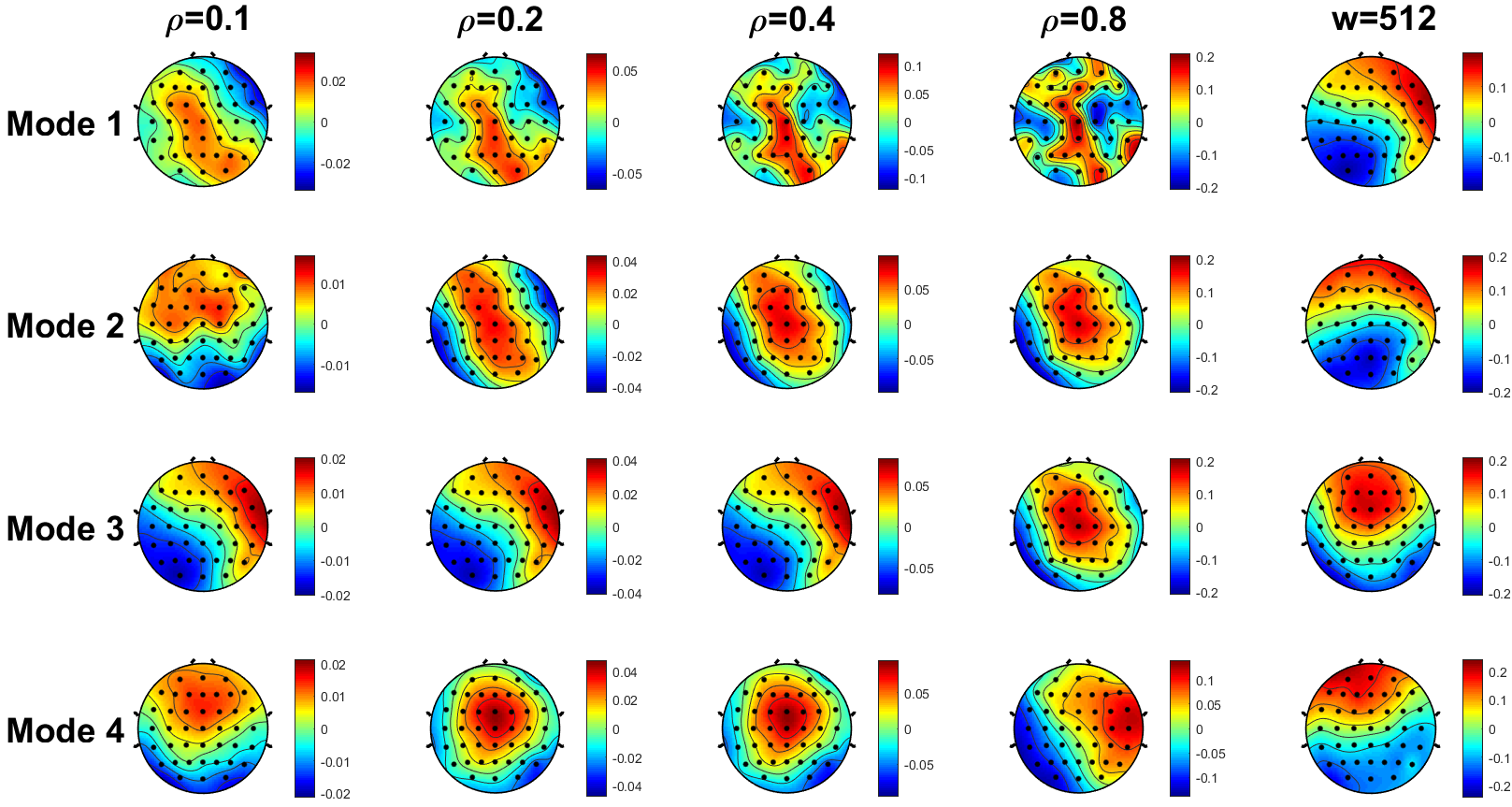
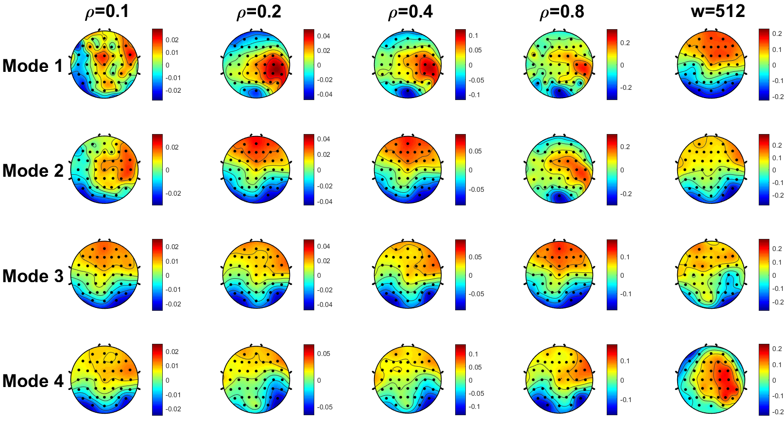
Topographical views for the real part of the four dominant DMD modes at 200 msec obtained from the incremental DMD algorithms for the correct and erroneous events are shown in Figure 7 and Figure 8, respectively. A comparison between the DMD modes during the erroneous and correct events shows that there is a stronger activity in the frontal lobe during the erroneous events especially around the FCz channel. This is consistent with the topographical views from EEG recordings shown in Figures 2a and 2b that show stronger activity in the frontal lobe during an erroneous event. This illustrates that a few principal DMD modes are able to capture the dominant activity in the brain during these experiments.
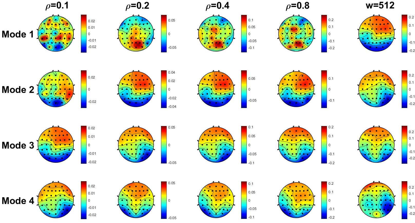
Refer to caption
(a) DMD modes σthr=0.01subscript𝜎thr0.01\sigma_{\text{thr}}=0.01.
Refer to caption
(b) DMD modes σthr=0.001subscript𝜎thr0.001\sigma_{\text{thr}}=0.001.
Fig. 7: Topographical views for the real part part of the 444 dominant DMD modes during correct events using threshold values of (a) σthr=0.01subscript𝜎thr0.01\sigma_{\text{thr}}=0.01, and (b) σthr=0.001subscript𝜎thr0.001\sigma_{\text{thr}}=0.001.
Refer to caption
(a) DMD modes σthr=0.01subscript𝜎thr0.01\sigma_{\text{thr}}=0.01.
Refer to caption
(b) DMD modes σthr=0.001subscript𝜎thr0.001\sigma_{\text{thr}}=0.001.
Fig. 8: Topographical views for the real part of the 444 dominant DMD modes during erroneous events using threshold values of (a) σthr=0.01subscript𝜎thr0.01\sigma_{\text{thr}}=0.01, and (b) σthr=0.001subscript𝜎thr0.001\sigma_{\text{thr}}=0.001.

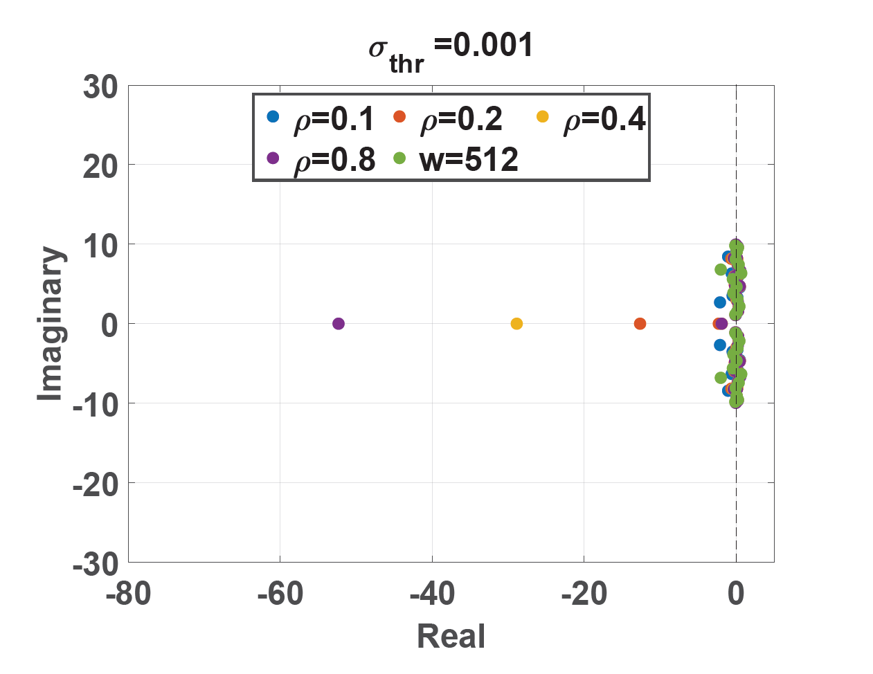
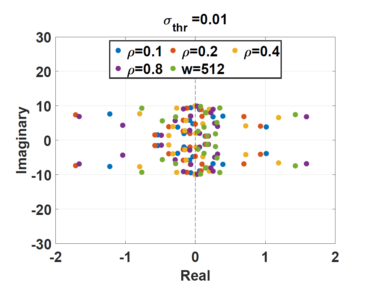
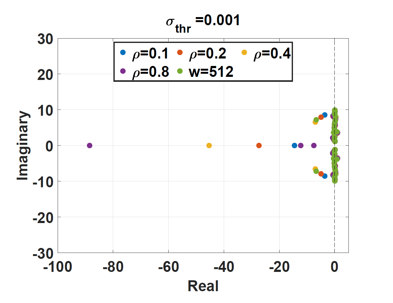
Figure 9 shows the logarithm of eigenvalues of the DMD operator at 200 msec associated with different thresholds σthrsubscript𝜎thr\sigma_{\text{thr}}, weight factor ρ𝜌\rho and time-window width. For smaller value of σthrsubscript𝜎thr\sigma_{\textup{thr}}, the range of eigenvalues in the left half plane is bigger. This is consistent with the fact that smaller σthrsubscript𝜎thr\sigma_{\text{thr}} implies a larger reduced order model in which some states converge to zero much faster than other states. For the erroneous event, some eigenvalues are spread in the right half plane, which suggest a locally unstable dynamics underlie the evolution of ERP signal during erroneous trials. This is also consistent with the faster dynamics (sharper peaks) in the EEG signal during the erroneous event (see Figure 2).
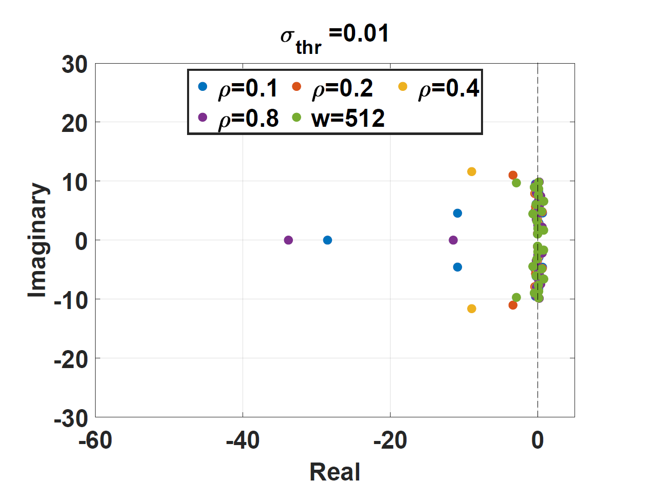
Refer to caption
Refer to caption
(a) Correct events
Refer to caption
Refer to caption
(b) Erroneous events
Fig. 9: The left panel show the continuous time DMD eigenvalues for σthr=0.01subscript𝜎thr0.01\sigma_{\text{thr}}=0.01 and the right panel shows the continuous time DMD eigenvalues for σthr=0.001subscript𝜎thr0.001\sigma_{\text{thr}}=0.001 during (a) correct events (b) erroneous events

We now investigate the effectiveness of the incremental DMD algorithms in terms of reconstructing the ERP signals during the correct and erroneous events at FCz channel. To this end, we reconstruct the signal starting from the onset of the events until the end of the third peak at 330330330 msec. The reconstructed signals and the normalized RMS error for the reconstruction are shown in Figures 10 and 11, respectively. These results indicate that the incremental DMD models incur smaller reconstruction error than the online DMD models. This result is counter-intuitive, since online DMD uses more modes and should lead to smaller reconstruction error. This discrepancy happens due to the fact that the data matrix never achieves full rank and the online DMD is not able to overcome the heuristic initialization discussed above. There is no significant difference in the reconstruction error for incremental DMD models with different ρ𝜌\rho and σthrsubscript𝜎thr\sigma_{\text{thr}} values as shown in Figure 10a.

Finally, we summarize the above investigation into the utility of incremental and online DMD in modeling EEG data. It appears that the pre-processing of the EEG data that requires domain-specific knowledge such as the band of frequency in which the event of interest is observed is vital to obtain sensible DMD-based data-driven models. However, after such pre-processing, the data matrix may become ill-conditioned and under such scenarios incremental DMD techniques proposed in this paper appear more promising that the online DMD techniques. There exists a trade-off between the threshold on the singular values used for model reduction and the window-width or the discount factor used in the incremental DMD algorithms. We also observed that the principal DMD modes are consistent with the activity in the brain during the studied experiments. This suggests that the incremental DMD algorithms can compute an efficient basis for describing the evolution of the EEG activity. Finally, we observed that under erroneous events, some DMD eigenvalues moved towards the right-half complex plane suggesting that certain events trigger (small time) unstable dynamics.
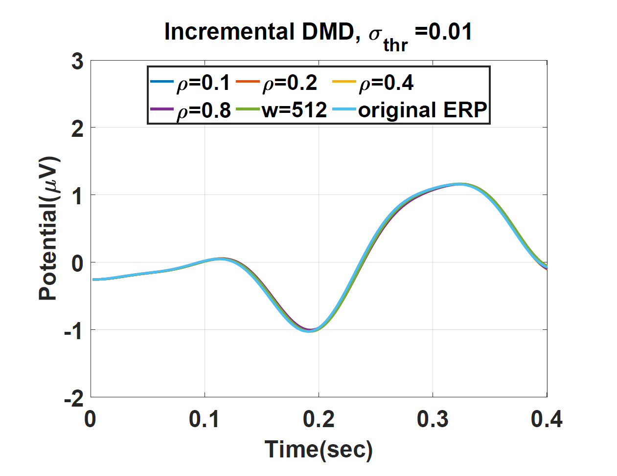
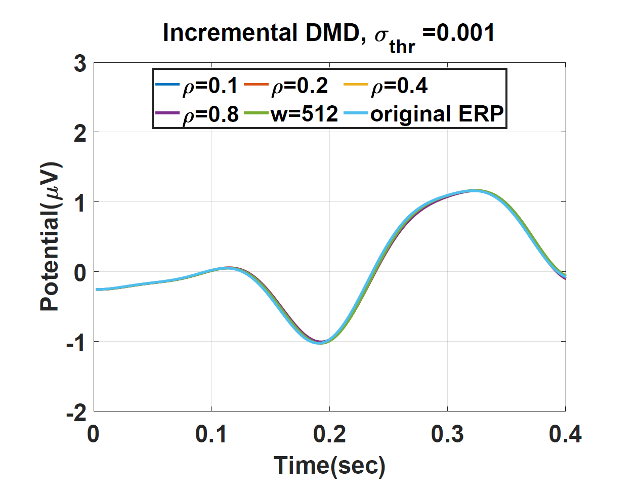
Refer to caption
Refer to caption
Refer to caption
(a) Correct event
Refer to caption
Refer to caption
Refer to caption
(b) Erroneous event
Fig. 10: Reconstructed ERP signal at channel FCz using incremental DMD with σthr=0.01subscript𝜎𝑡𝑟0.01\sigma_{thr}=0.01 (left panel), incremental DMD with σthr=0.001subscript𝜎𝑡𝑟0.001\sigma_{thr}=0.001 (middle panel), and online DMD (right panel) for (a) correct events and (b) erroneous events.
Refer to caption
Refer to caption
(a) Incremental DMD
Refer to caption
Refer to caption
(b) Online DMD
Fig. 11: Normalized RMS error for the reconstructed ERP signal at channel FCz for correct events (left panel) and erroneous events (right panel), using (a) incremental DMD, and (b) online DMD.

6 Incremental Dynamic Mode Decomposition for Systems with Control Input

In this section, we extended the incremental DMD algorithms to the case of non-autonomous dynamical systems. We first recall the Dynamic Mode Decomposition with Control (DMDc) algorithm proposed in [27] that estimates time-invariant non-autonomous system dynamics underlying high-dimensional data.

For the scenarios in which the non-autonomous system underlying the measurements is time-varying, the DMDc algorithm has been extended to the online DMDc algorithm [35]. The online DMDc algorithm operates similarly to the online DMD algorithm and yields time-varying matrices 𝐀kcn×nsubscriptsuperscript𝐀𝑐𝑘superscript𝑛𝑛\mathbf{A}^{c}_{k}\in\mathbb{R}^{n\times n} and 𝐁kcn×lsubscriptsuperscript𝐁𝑐𝑘superscript𝑛𝑙\mathbf{B}^{c}_{k}\in\mathbb{R}^{n\times l}, k{1,2,}𝑘12k\in\{1,2,\cdots\}. Similar to the online DMD algorithm, the DMDc algorithm also does not allow for incremental computation of the lower dimensional non-autonomous system underlying high dimensional measurements. In the following, we extend the DMDc algorithm to the weighted and windowed incremental DMDc algorithms that enable us to obtain a lower-dimensional time-varying approximation for the underlying dynamics.

6.1 Weighted Incremental DMDc Algorithm

Assume that at sampling time tk+1subscript𝑡𝑘1t_{k+1}, the measurements and the associated exogeneous inputs are arranged in the following datasets

𝐗ksubscript𝐗𝑘\displaystyle\mathbf{X}_{k} =[ρk1𝐱1ρk2𝐱2𝐱k],𝐘k=[ρk1𝐲1ρk2𝐲2𝐲k]formulae-sequenceabsentmatrixsuperscript𝜌𝑘1subscript𝐱1superscript𝜌𝑘2subscript𝐱2subscript𝐱𝑘subscript𝐘𝑘matrixsuperscript𝜌𝑘1subscript𝐲1superscript𝜌𝑘2subscript𝐲2subscript𝐲𝑘\displaystyle=\begin{bmatrix}\rho^{k-1}\mathbf{x}_{1}&\rho^{k-2}\mathbf{x}_{2}&\cdots&\mathbf{x}_{k}\end{bmatrix},\mathbf{Y}_{k}=\begin{bmatrix}\rho^{k-1}\mathbf{y}_{1}&\rho^{k-2}\mathbf{y}_{2}&\cdots&\mathbf{y}_{k}\end{bmatrix} (41)
𝚪ksubscript𝚪𝑘\displaystyle\mathbf{\Gamma}_{k} =[ρk1𝜸1ρk2𝜸2𝜸k],𝐗kc=[𝐗k𝚪k]formulae-sequenceabsentmatrixsuperscript𝜌𝑘1subscript𝜸1superscript𝜌𝑘2subscript𝜸2subscript𝜸𝑘superscriptsubscript𝐗𝑘𝑐superscriptmatrixsuperscriptsubscript𝐗𝑘superscriptsubscript𝚪𝑘\displaystyle=\begin{bmatrix}\rho^{k-1}\boldsymbol{\gamma}_{1}&\rho^{k-2}\boldsymbol{\gamma}_{2}&\cdots&\boldsymbol{\gamma}_{k}\end{bmatrix},\mathbf{X}_{k}^{c}=\begin{bmatrix}\mathbf{X}_{k}^{*}&\mathbf{\Gamma}_{k}^{*}\end{bmatrix}^{*}

respectively, where 𝐗k,𝐘kn×ksubscript𝐗𝑘subscript𝐘𝑘superscript𝑛𝑘\mathbf{X}_{k},\mathbf{Y}_{k}\in\mathbb{R}^{n\times k}, 𝚪kl×ksubscript𝚪𝑘superscript𝑙𝑘\mathbf{\Gamma}_{k}\in\mathbb{R}^{l\times k}, and 𝐗kc(n+l)×ksuperscriptsubscript𝐗𝑘𝑐superscript𝑛𝑙𝑘\mathbf{X}_{k}^{c}\in\mathbb{R}^{(n+l)\times k}. At sampling time tk+1subscript𝑡𝑘1t_{k+1}, the datasets are updated with a new set of measurements (𝐱k+1,𝐲k+1,𝜸k+1)subscript𝐱𝑘1subscript𝐲𝑘1subscript𝜸𝑘1\left(\mathbf{x}_{k+1},\mathbf{y}_{k+1},\boldsymbol{\gamma}_{k+1}\right) which results in the following

𝐗k+1subscript𝐗𝑘1\displaystyle\mathbf{X}_{k+1} =[ρ𝐗k𝐱k+1],𝐘k+1=[ρ𝐘k𝐲k+1],formulae-sequenceabsentmatrix𝜌subscript𝐗𝑘subscript𝐱𝑘1subscript𝐘𝑘1matrix𝜌subscript𝐘𝑘subscript𝐲𝑘1\displaystyle=\begin{bmatrix}\rho\mathbf{X}_{k}&\mathbf{x}_{k+1}\end{bmatrix},\mathbf{Y}_{k+1}=\begin{bmatrix}\rho\mathbf{Y}_{k}&\mathbf{y}_{k+1}\end{bmatrix}, (42)
𝚪k+1subscript𝚪𝑘1\displaystyle\mathbf{\Gamma}_{k+1} =[ρ𝚪k𝜸k+1],𝐗k+1c=[𝐗k+1𝚪k+1].formulae-sequenceabsentmatrix𝜌subscript𝚪𝑘subscript𝜸𝑘1superscriptsubscript𝐗𝑘1𝑐superscriptmatrixsuperscriptsubscript𝐗𝑘1superscriptsubscript𝚪𝑘1\displaystyle=\begin{bmatrix}\rho\mathbf{\Gamma}_{k}&\boldsymbol{\gamma}_{k+1}\end{bmatrix},\mathbf{X}_{k+1}^{c}=\begin{bmatrix}\mathbf{X}_{k+1}^{*}&\mathbf{\Gamma}_{k+1}^{*}\end{bmatrix}^{*}.

Suppose that the weighted DMDc operator and input matrix at tk+1subscript𝑡𝑘1t_{k+1}, and the SVD of both 𝐗ksubscript𝐗𝑘\mathbf{X}_{k} and 𝐗kcsuperscriptsubscript𝐗𝑘𝑐\mathbf{X}_{k}^{c} are known, then according to the new incoming measurements at tk+2subscript𝑡𝑘2t_{k+2}, the updates for the weighted DMDc operator and input matrix can be obtained using the following theorem, which is proved in Appendix G.

Theorem 3.

Let at sampling time tk+1subscript𝑡𝑘1t_{k+1} the SVD of 𝐗kc=𝐔xkc𝚺xkc𝐕xkcsubscriptsuperscript𝐗𝑐𝑘subscriptsuperscript𝐔𝑐subscript𝑥𝑘subscriptsuperscript𝚺𝑐subscript𝑥𝑘subscriptsuperscript𝐕𝑐subscript𝑥𝑘\mathbf{X}^{c}_{k}=\mathbf{U}^{c}_{x_{k}}\mathbf{\Sigma}^{c}_{x_{k}}\mathbf{V}^{c*}_{x_{k}} and 𝐗k=𝐔xk𝚺xk𝐕xksubscript𝐗𝑘subscript𝐔subscript𝑥𝑘subscript𝚺subscript𝑥𝑘subscriptsuperscript𝐕subscript𝑥𝑘\mathbf{X}_{k}=\mathbf{U}_{x_{k}}\mathbf{\Sigma}_{x_{k}}\mathbf{V}^{*}_{x_{k}} be known. Assume that the pair (𝐀kρc,𝐁kρc)subscriptsuperscript𝐀subscript𝜌𝑐𝑘subscriptsuperscript𝐁subscript𝜌𝑐𝑘(\mathbf{A}^{\rho_{c}}_{k},\mathbf{B}^{\rho_{c}}_{k}) minimizes the cost function in (11) with 𝐗ksubscript𝐗𝑘\mathbf{X}_{k} and 𝚪ksubscript𝚪𝑘\mathbf{\Gamma}_{k} defined in (41). Consider that at sampling time tk+2subscript𝑡𝑘2t_{k+2}, a new triplet of measurements (𝐱k+1,𝐲k+1,𝛄k+1)subscript𝐱𝑘1subscript𝐲𝑘1subscript𝛄𝑘1(\mathbf{x}_{k+1},\mathbf{y}_{k+1},\boldsymbol{\gamma}_{k+1}) is used to incrementally compute the SVD of both 𝐗k+1csuperscriptsubscript𝐗𝑘1𝑐\mathbf{X}_{k+1}^{c} and 𝐗k+1subscript𝐗𝑘1\mathbf{X}_{k+1} using Proposition 1. Then, the pair (𝐀k+1ρc,𝐁k+1ρc)subscriptsuperscript𝐀subscript𝜌𝑐𝑘1subscriptsuperscript𝐁subscript𝜌𝑐𝑘1(\mathbf{A}^{\rho_{c}}_{k+1},\mathbf{B}^{\rho_{c}}_{k+1}) which minimizes the cost function in (11) is

𝐀k+1ρc=𝐀kρc+(𝐲k+1𝐀kρc𝐱k+1𝐁kρc𝜸k+1)𝐯sk,2c(𝚺xk+1c)1𝐔xk+1ca,𝐁k+1ρc=𝐁kρc+(𝐲k+1𝐀kρc𝐱k+1𝐁kρc𝜸k+1)𝐯sk,2c(𝚺xk+1c)1𝐔xk+1cb.formulae-sequencesubscriptsuperscript𝐀subscript𝜌𝑐𝑘1subscriptsuperscript𝐀subscript𝜌𝑐𝑘subscript𝐲𝑘1subscriptsuperscript𝐀subscript𝜌𝑐𝑘subscript𝐱𝑘1subscriptsuperscript𝐁subscript𝜌𝑐𝑘subscript𝜸𝑘1subscriptsuperscript𝐯𝑐subscript𝑠𝑘2superscriptsubscriptsuperscript𝚺𝑐subscript𝑥𝑘11subscriptsuperscript𝐔subscript𝑐𝑎subscript𝑥𝑘1subscriptsuperscript𝐁subscript𝜌𝑐𝑘1subscriptsuperscript𝐁subscript𝜌𝑐𝑘subscript𝐲𝑘1subscriptsuperscript𝐀subscript𝜌𝑐𝑘subscript𝐱𝑘1subscriptsuperscript𝐁subscript𝜌𝑐𝑘subscript𝜸𝑘1subscriptsuperscript𝐯𝑐subscript𝑠𝑘2superscriptsubscriptsuperscript𝚺𝑐subscript𝑥𝑘11subscriptsuperscript𝐔subscript𝑐𝑏subscript𝑥𝑘1\displaystyle\begin{split}{\mathbf{A}}^{\rho_{c}}_{k+1}&={\mathbf{A}}^{\rho_{c}}_{k}+\left(\mathbf{y}_{k+1}-{\mathbf{A}}^{\rho_{c}}_{k}\mathbf{x}_{k+1}-{\mathbf{B}}^{\rho_{c}}_{k}\boldsymbol{\gamma}_{k+1}\right){\mathbf{v}}^{c}_{s_{k,2}}({\mathbf{\Sigma}}^{c}_{x_{k+1}})^{-1}{\mathbf{U}}^{c_{a}*}_{x_{k+1}},\\ {\mathbf{B}}^{\rho_{c}}_{k+1}&={\mathbf{B}}^{\rho_{c}}_{k}+\left(\mathbf{y}_{k+1}-{\mathbf{A}}^{\rho_{c}}_{k}\mathbf{x}_{k+1}-{\mathbf{B}}^{\rho_{c}}_{k}\boldsymbol{\gamma}_{k+1}\right){\mathbf{v}}^{c}_{s_{k,2}}({\mathbf{\Sigma}}^{c}_{x_{k+1}})^{-1}{\mathbf{U}}^{c_{b}*}_{x_{k+1}}.\end{split} (43)

Assume that 𝐗k+1csubscriptsuperscript𝐗𝑐𝑘1\mathbf{X}^{c}_{k+1} can be well-approximated by its projection onto its leading p𝑝p singular vectors such that 𝐗k+1c𝐗¯k+1c=𝐔¯xk+1c𝚺¯xk+1c𝐕¯xk+1csubscriptsuperscript𝐗𝑐𝑘1subscriptsuperscript¯𝐗𝑐𝑘1subscriptsuperscript¯𝐔𝑐subscript𝑥𝑘1subscriptsuperscript¯𝚺𝑐subscript𝑥𝑘1subscriptsuperscript¯𝐕𝑐subscript𝑥𝑘1\mathbf{X}^{c}_{k+1}\approx\bar{\mathbf{X}}^{c}_{k+1}=\bar{\mathbf{U}}^{c}_{x_{k+1}}\bar{\mathbf{\Sigma}}^{c}_{x_{k+1}}\bar{\mathbf{V}}^{c*}_{x_{k+1}}, where 𝐔¯xk+1c(n+l)×psuperscriptsubscript¯𝐔subscript𝑥𝑘1𝑐superscript𝑛𝑙𝑝\bar{\mathbf{U}}_{x_{k+1}}^{c}\in\mathbb{C}^{(n+l)\times p}, 𝚺¯xk+1cp×psuperscriptsubscript¯𝚺subscript𝑥𝑘1𝑐superscript𝑝𝑝\bar{\mathbf{\Sigma}}_{x_{k+1}}^{c}\in\mathbb{C}^{p\times p} ,and 𝐕¯xk+1c(k+1)×psuperscriptsubscript¯𝐕subscript𝑥𝑘1𝑐superscript𝑘1𝑝\bar{\mathbf{V}}_{x_{k+1}}^{c}\in\mathbb{C}^{(k+1)\times p}. Let 𝐔¯xk+1csuperscriptsubscript¯𝐔subscript𝑥𝑘1𝑐\bar{\mathbf{U}}_{x_{k+1}}^{c*} be partitioned such that 𝐔¯xk+1c=[𝐔¯xk+1ca𝐔¯xk+1cb]superscriptsubscript¯𝐔subscript𝑥𝑘1𝑐delimited-[]subscriptsuperscript¯𝐔subscript𝑐𝑎subscript𝑥𝑘1subscriptsuperscript¯𝐔subscript𝑐𝑏subscript𝑥𝑘1\bar{\mathbf{U}}_{x_{k+1}}^{c*}=[\bar{\mathbf{U}}^{c_{a}*}_{x_{k+1}}\bar{\mathbf{U}}^{c_{b}*}_{x_{k+1}}], where 𝐔¯xk+1can×psubscriptsuperscript¯𝐔subscript𝑐𝑎subscript𝑥𝑘1superscript𝑛𝑝\bar{\mathbf{U}}^{c_{a}}_{x_{k+1}}\in\mathbb{C}^{n\times p} and 𝐔¯xk+1cbl×psubscriptsuperscript¯𝐔subscript𝑐𝑏subscript𝑥𝑘1superscript𝑙𝑝\bar{\mathbf{U}}^{c_{b}}_{x_{k+1}}\in\mathbb{C}^{l\times p}. Then, the update in (43) yields the following updates for 𝐀¯k+1ρcn×nsubscriptsuperscript¯𝐀subscript𝜌𝑐𝑘1superscript𝑛𝑛\bar{\mathbf{A}}^{\rho_{c}}_{k+1}\in\mathbb{R}^{n\times n} and 𝐁¯k+1ρcn×lsubscriptsuperscript¯𝐁subscript𝜌𝑐𝑘1superscript𝑛𝑙\bar{\mathbf{B}}^{\rho_{c}}_{k+1}\in\mathbb{R}^{n\times l}:

𝐀¯k+1ρcsubscriptsuperscript¯𝐀subscript𝜌𝑐𝑘1\displaystyle\bar{\mathbf{A}}^{\rho_{c}}_{k+1} =𝐀¯kρc+(𝐲k+1𝐀¯kρc𝐱k+1𝐁¯kρc𝜸k+1)𝐯¯sk,2c(𝚺¯xk+1c)1𝐔¯xk+1caabsentsubscriptsuperscript¯𝐀subscript𝜌𝑐𝑘subscript𝐲𝑘1subscriptsuperscript¯𝐀subscript𝜌𝑐𝑘subscript𝐱𝑘1subscriptsuperscript¯𝐁subscript𝜌𝑐𝑘subscript𝜸𝑘1subscriptsuperscript¯𝐯𝑐subscript𝑠𝑘2superscriptsubscriptsuperscript¯𝚺𝑐subscript𝑥𝑘11subscriptsuperscript¯𝐔subscript𝑐𝑎subscript𝑥𝑘1\displaystyle=\bar{\mathbf{A}}^{\rho_{c}}_{k}+\left(\mathbf{y}_{k+1}-\bar{\mathbf{A}}^{\rho_{c}}_{k}\mathbf{x}_{k+1}-\bar{\mathbf{B}}^{\rho_{c}}_{k}\boldsymbol{\gamma}_{k+1}\right)\bar{\mathbf{v}}^{c}_{s_{k,2}}(\bar{\mathbf{\Sigma}}^{c}_{x_{k+1}})^{-1}\bar{\mathbf{U}}^{c_{a}*}_{x_{k+1}}
𝐁¯k+1ρcsubscriptsuperscript¯𝐁subscript𝜌𝑐𝑘1\displaystyle\bar{\mathbf{B}}^{\rho_{c}}_{k+1} =𝐁¯kρc+(𝐲k+1𝐀¯kρc𝐱k+1𝐁¯kρc𝜸k+1)𝐯¯sk,2c(𝚺¯xk+1c)1𝐔¯xk+1cb.absentsubscriptsuperscript¯𝐁subscript𝜌𝑐𝑘subscript𝐲𝑘1subscriptsuperscript¯𝐀subscript𝜌𝑐𝑘subscript𝐱𝑘1subscriptsuperscript¯𝐁subscript𝜌𝑐𝑘subscript𝜸𝑘1subscriptsuperscript¯𝐯𝑐subscript𝑠𝑘2superscriptsubscriptsuperscript¯𝚺𝑐subscript𝑥𝑘11subscriptsuperscript¯𝐔subscript𝑐𝑏subscript𝑥𝑘1\displaystyle=\bar{\mathbf{B}}^{\rho_{c}}_{k}+\left(\mathbf{y}_{k+1}-\bar{\mathbf{A}}^{\rho_{c}}_{k}\mathbf{x}_{k+1}-\bar{\mathbf{B}}^{\rho_{c}}_{k}\boldsymbol{\gamma}_{k+1}\right)\bar{\mathbf{v}}^{c}_{s_{k,2}}(\bar{\mathbf{\Sigma}}^{c}_{x_{k+1}})^{-1}\bar{\mathbf{U}}^{c_{b}*}_{x_{k+1}}.

Assume that 𝐗k+1subscript𝐗𝑘1\mathbf{X}_{k+1} is well-approximated by its projection onto its leading r𝑟r singular vectors such that 𝐗k+1𝐗¯k+1=𝐔¯xk+1𝚺¯xk+1𝐕¯xk+1subscript𝐗𝑘1subscript¯𝐗𝑘1subscript¯𝐔subscript𝑥𝑘1subscript¯𝚺subscript𝑥𝑘1subscriptsuperscript¯𝐕subscript𝑥𝑘1\mathbf{X}_{k+1}\approx\bar{\mathbf{X}}_{k+1}=\bar{\mathbf{U}}_{x_{k+1}}\bar{\mathbf{\Sigma}}_{x_{k+1}}\bar{\mathbf{V}}^{*}_{x_{k+1}} with rp𝑟𝑝r\leq p. Then a reduced order model can be represented as:

𝐱~k+1=𝐀~kρc𝐱~k+𝐁~kρcγk,subscript~𝐱𝑘1subscriptsuperscript~𝐀subscript𝜌𝑐𝑘subscript~𝐱𝑘subscriptsuperscript~𝐁subscript𝜌𝑐𝑘subscript𝛾𝑘\displaystyle\tilde{\mathbf{x}}_{k+1}=\tilde{\mathbf{A}}^{\rho_{c}}_{k}\tilde{\mathbf{x}}_{k}+\tilde{\mathbf{B}}^{\rho_{c}}_{k}{\gamma}_{k},

where the lower-dimensional approximation 𝐀~k+1ρcr×rsubscriptsuperscript~𝐀subscript𝜌𝑐𝑘1superscript𝑟𝑟\tilde{\mathbf{A}}^{\rho_{c}}_{k+1}\in\mathbb{R}^{r\times r} and 𝐁~k+1ρcr×lsubscriptsuperscript~𝐁subscript𝜌𝑐𝑘1superscript𝑟𝑙\tilde{\mathbf{B}}^{\rho_{c}}_{k+1}\in\mathbb{R}^{r\times l} can obtained by projecting 𝐀¯k+1ρcsubscriptsuperscript¯𝐀subscript𝜌𝑐𝑘1\bar{\mathbf{A}}^{\rho_{c}}_{k+1} and 𝐁¯k+1ρcsubscriptsuperscript¯𝐁subscript𝜌𝑐𝑘1\bar{\mathbf{B}}^{\rho_{c}}_{k+1} onto a subspace spanned by the columns of 𝐔¯xk+1subscript¯𝐔subscript𝑥𝑘1\bar{\mathbf{U}}_{x_{k+1}} as follows:

𝐀~k+1ρcsubscriptsuperscript~𝐀subscript𝜌𝑐𝑘1\displaystyle\tilde{\mathbf{A}}^{\rho_{c}}_{k+1} =𝐔¯xk+1𝐀¯kρc𝐔¯xk+1+𝐔¯xk+1(𝐲k+1𝐀¯kρc𝐱k+1𝐁¯kρc𝜸k+1)𝐯¯sk,2c(𝚺¯xk+1c)1𝐔¯xk+1ca𝐔¯xk+1absentsubscriptsuperscript¯𝐔subscript𝑥𝑘1subscriptsuperscript¯𝐀subscript𝜌𝑐𝑘subscript¯𝐔subscript𝑥𝑘1subscriptsuperscript¯𝐔subscript𝑥𝑘1subscript𝐲𝑘1subscriptsuperscript¯𝐀subscript𝜌𝑐𝑘subscript𝐱𝑘1subscriptsuperscript¯𝐁subscript𝜌𝑐𝑘subscript𝜸𝑘1subscriptsuperscript¯𝐯𝑐subscript𝑠𝑘2superscriptsubscriptsuperscript¯𝚺𝑐subscript𝑥𝑘11subscriptsuperscript¯𝐔subscript𝑐𝑎subscript𝑥𝑘1subscript¯𝐔subscript𝑥𝑘1\displaystyle=\bar{\mathbf{U}}^{*}_{x_{k+1}}\bar{\mathbf{A}}^{\rho_{c}}_{k}\bar{\mathbf{U}}_{x_{k+1}}+\bar{\mathbf{U}}^{*}_{x_{k+1}}\left(\mathbf{y}_{k+1}-\bar{\mathbf{A}}^{\rho_{c}}_{k}\mathbf{x}_{k+1}-\bar{\mathbf{B}}^{\rho_{c}}_{k}\boldsymbol{\gamma}_{k+1}\right)\bar{\mathbf{v}}^{c}_{s_{k,2}}(\bar{\mathbf{\Sigma}}^{c}_{x_{k+1}})^{-1}\bar{\mathbf{U}}^{c_{a}*}_{x_{k+1}}\bar{\mathbf{U}}_{x_{k+1}}
𝐁~k+1ρcsubscriptsuperscript~𝐁subscript𝜌𝑐𝑘1\displaystyle\tilde{\mathbf{B}}^{\rho_{c}}_{k+1} =𝐔¯xk+1𝐁¯kρc+𝐔¯xk+1(𝐲k+1𝐀¯kρc𝐱k+1𝐁¯kρc𝜸k+1)𝐯¯sk,2c(𝚺¯xk+1c)1𝐔¯xk+1cb.absentsubscriptsuperscript¯𝐔subscript𝑥𝑘1subscriptsuperscript¯𝐁subscript𝜌𝑐𝑘subscriptsuperscript¯𝐔subscript𝑥𝑘1subscript𝐲𝑘1subscriptsuperscript¯𝐀subscript𝜌𝑐𝑘subscript𝐱𝑘1subscriptsuperscript¯𝐁subscript𝜌𝑐𝑘subscript𝜸𝑘1subscriptsuperscript¯𝐯𝑐subscript𝑠𝑘2superscriptsubscriptsuperscript¯𝚺𝑐subscript𝑥𝑘11subscriptsuperscript¯𝐔subscript𝑐𝑏subscript𝑥𝑘1\displaystyle=\bar{\mathbf{U}}^{*}_{x_{k+1}}\bar{\mathbf{B}}^{\rho_{c}}_{k}+\bar{\mathbf{U}}^{*}_{x_{k+1}}\left(\mathbf{y}_{k+1}-\bar{\mathbf{A}}^{\rho_{c}}_{k}\mathbf{x}_{k+1}-\bar{\mathbf{B}}^{\rho_{c}}_{k}\boldsymbol{\gamma}_{k+1}\right)\bar{\mathbf{v}}^{c}_{s_{k,2}}(\bar{\mathbf{\Sigma}}^{c}_{x_{k+1}})^{-1}\bar{\mathbf{U}}^{c_{b}*}_{x_{k+1}}.

The update in equation (43) requires only the current DMD operator (𝐀kρc,𝐁kρc)subscriptsuperscript𝐀subscript𝜌𝑐𝑘subscriptsuperscript𝐁subscript𝜌𝑐𝑘(\mathbf{A}^{\rho_{c}}_{k},\mathbf{B}^{\rho_{c}}_{k}), measurements set of (𝐲k+1,𝐱k+1,γk+1)subscript𝐲𝑘1subscript𝐱𝑘1subscript𝛾𝑘1(\mathbf{y}_{k+1},\mathbf{x}_{k+1},{\gamma}_{k+1}), and the incremental SVD update. Specifically, these updates do not require the large data matrix to be stored.

6.2 Windowed Incremental DMDc Algorithm

Assume that at sampling time tk+1subscript𝑡𝑘1t_{k+1}, the past w𝑤w states and control input measurements are arranged in the following datasets

𝝌ksubscript𝝌𝑘\displaystyle\boldsymbol{\chi}_{k} =[𝐱kw+1𝐱k],𝚼k=[𝐲kw+1𝐲k],formulae-sequenceabsentmatrixsubscript𝐱𝑘𝑤1subscript𝐱𝑘subscript𝚼𝑘matrixsubscript𝐲𝑘𝑤1subscript𝐲𝑘\displaystyle=\begin{bmatrix}\mathbf{x}_{k-w+1}&\cdots&\mathbf{x}_{k}\end{bmatrix},\boldsymbol{\Upsilon}_{k}=\begin{bmatrix}\mathbf{y}_{k-w+1}&\cdots&\mathbf{y}_{k}\end{bmatrix}, (44)
𝚪ksubscript𝚪𝑘\displaystyle\mathbf{\Gamma}_{k} =[𝜸kw+1𝜸k],𝝌kc=[𝝌k𝚪k],formulae-sequenceabsentmatrixsubscript𝜸𝑘𝑤1subscript𝜸𝑘subscriptsuperscript𝝌𝑐𝑘superscriptmatrixsuperscriptsubscript𝝌𝑘superscriptsubscript𝚪𝑘\displaystyle=\begin{bmatrix}\boldsymbol{\gamma}_{k-w+1}&\cdots&\boldsymbol{\gamma}_{k}\end{bmatrix},\boldsymbol{\chi}^{c}_{k}=\begin{bmatrix}\boldsymbol{\chi}_{k}^{*}&\mathbf{\Gamma}_{k}^{*}\end{bmatrix}^{*},

where 𝝌k,𝚼kn×wsubscript𝝌𝑘subscript𝚼𝑘superscript𝑛𝑤\boldsymbol{\chi}_{k},\boldsymbol{\Upsilon}_{k}\in\mathbb{R}^{n\times w}, 𝚪ll×wsubscript𝚪𝑙superscript𝑙𝑤\mathbf{\Gamma}_{l}\in\mathbb{R}^{l\times w}, and 𝝌kc(n+l)×wsubscriptsuperscript𝝌𝑐𝑘superscript𝑛𝑙𝑤\boldsymbol{\chi}^{c}_{k}\in\mathbb{R}^{(n+l)\times w}, respectively. At sampling time tk+1subscript𝑡𝑘1t_{k+1}, the datasets are updated by adding a new set of measurements (𝐱k+1,𝐲k+1,𝜸k+1)subscript𝐱𝑘1subscript𝐲𝑘1subscript𝜸𝑘1\left(\mathbf{x}_{k+1},\mathbf{y}_{k+1},\boldsymbol{\gamma}_{k+1}\right), and removing the oldest set of measurements (𝐱kw+1,𝐲kw+1,𝜸kw+1)subscript𝐱𝑘𝑤1subscript𝐲𝑘𝑤1subscript𝜸𝑘𝑤1\left(\mathbf{x}_{k-w+1},\mathbf{y}_{k-w+1},\boldsymbol{\gamma}_{k-w+1}\right), such that:

𝝌k+1subscript𝝌𝑘1\displaystyle\boldsymbol{\chi}_{k+1} =[𝐱kw+2𝐱k+1],𝚼k+1=[𝐲kw+2𝐲k+1],formulae-sequenceabsentmatrixsubscript𝐱𝑘𝑤2subscript𝐱𝑘1subscript𝚼𝑘1matrixsubscript𝐲𝑘𝑤2subscript𝐲𝑘1\displaystyle=\begin{bmatrix}\mathbf{x}_{k-w+2}&\cdots&\mathbf{x}_{k+1}\end{bmatrix},\boldsymbol{\Upsilon}_{k+1}=\begin{bmatrix}\mathbf{y}_{k-w+2}&\cdots&\mathbf{y}_{k+1}\end{bmatrix}, (45)
𝚪k+1subscript𝚪𝑘1\displaystyle\mathbf{\Gamma}_{k+1} =[𝜸kw+2𝜸k+1],𝝌k+1c=[𝝌k+1𝚪k+1].formulae-sequenceabsentmatrixsubscript𝜸𝑘𝑤2subscript𝜸𝑘1subscriptsuperscript𝝌𝑐𝑘1superscriptmatrixsuperscriptsubscript𝝌𝑘1superscriptsubscript𝚪𝑘1\displaystyle=\begin{bmatrix}\boldsymbol{\gamma}_{k-w+2}&\cdots&\boldsymbol{\gamma}_{k+1}\end{bmatrix},\boldsymbol{\chi}^{c}_{k+1}=\begin{bmatrix}\boldsymbol{\chi}_{k+1}^{*}&\mathbf{\Gamma}_{k+1}^{*}\end{bmatrix}^{*}.

Suppose that the windowed DMDc operator and input matrix at tk+1subscript𝑡𝑘1t_{k+1}, and the SVD of both 𝝌ksubscript𝝌𝑘\boldsymbol{\chi}_{k} and 𝝌kcsubscriptsuperscript𝝌𝑐𝑘\boldsymbol{\chi}^{c}_{k} are known. Then, according to the new incoming measurements at tk+2subscript𝑡𝑘2t_{k+2}, the updates for the windowed DMDc operator and input matrix can be obtained using the following theorem, which is proved in Appendix H.

Theorem 4.

Let at sampling time tk+1subscript𝑡𝑘1t_{k+1} the SVD of 𝛘k=𝐔χk𝚺χk𝐕χksubscript𝛘𝑘subscript𝐔subscript𝜒𝑘subscript𝚺subscript𝜒𝑘subscriptsuperscript𝐕subscript𝜒𝑘\boldsymbol{\chi}_{k}=\mathbf{U}_{\chi_{k}}\mathbf{\Sigma}_{\chi_{k}}\mathbf{V}^{*}_{\chi_{k}} and 𝛘kc=𝐔χkc𝚺χkc𝐕χkcsuperscriptsubscript𝛘𝑘𝑐subscriptsuperscript𝐔𝑐subscript𝜒𝑘subscriptsuperscript𝚺𝑐subscript𝜒𝑘subscriptsuperscript𝐕𝑐subscript𝜒𝑘\boldsymbol{\chi}_{k}^{c}=\mathbf{U}^{c}_{\chi_{k}}\mathbf{\Sigma}^{c}_{\chi_{k}}\mathbf{V}^{c*}_{\chi_{k}} be known, and let the pair (𝐀kwc,𝐁kwc)subscriptsuperscript𝐀subscript𝑤𝑐𝑘subscriptsuperscript𝐁subscript𝑤𝑐𝑘(\mathbf{A}^{w_{c}}_{k},\mathbf{B}^{w_{c}}_{k}) minimize the cost function in (11) with 𝚼ksubscript𝚼𝑘\boldsymbol{\Upsilon}_{k} and 𝛘ksubscript𝛘𝑘\boldsymbol{\chi}_{k} given in (44). Assume that at sampling time tk+2subscript𝑡𝑘2t_{k+2}, a new triplet of measurements (𝐱k+1,𝐲k+1,𝛄k+1)subscript𝐱𝑘1subscript𝐲𝑘1subscript𝛄𝑘1(\mathbf{x}_{k+1},\mathbf{y}_{k+1},\boldsymbol{\gamma}_{k+1}) is used to incrementally compute the SVD of 𝛘k+1csubscriptsuperscript𝛘𝑐𝑘1\boldsymbol{\chi}^{c}_{k+1} and 𝛘k+1subscript𝛘𝑘1\boldsymbol{\chi}_{k+1} using Proposition 2 and equation (3.2). Then, the pair (𝐀k+1wc,𝐁k+1wc)subscriptsuperscript𝐀subscript𝑤𝑐𝑘1subscriptsuperscript𝐁subscript𝑤𝑐𝑘1(\mathbf{A}^{w_{c}}_{k+1},\mathbf{B}^{w_{c}}_{k+1}) which minimizes the cost function in (11) is

𝐀k+1wc=𝐀kwc+(𝐲k+1𝐀kwc𝐱k+1𝐁kwc𝜸k+1)𝐯s^k,2c(𝚺χk+1c)1𝐔χk+1ca,𝐁k+1wc=𝐁kwc+(𝐲k+1𝐀kwc𝐱k+1𝐁kwc𝜸k+1)𝐯s^k,2c(𝚺χk+1c)1𝐔χk+1cb.formulae-sequencesubscriptsuperscript𝐀subscript𝑤𝑐𝑘1subscriptsuperscript𝐀subscript𝑤𝑐𝑘subscript𝐲𝑘1subscriptsuperscript𝐀subscript𝑤𝑐𝑘subscript𝐱𝑘1subscriptsuperscript𝐁subscript𝑤𝑐𝑘subscript𝜸𝑘1superscriptsubscript𝐯subscript^𝑠𝑘2𝑐superscriptsubscriptsuperscript𝚺𝑐subscript𝜒𝑘11subscriptsuperscript𝐔subscript𝑐𝑎subscript𝜒𝑘1subscriptsuperscript𝐁subscript𝑤𝑐𝑘1subscriptsuperscript𝐁subscript𝑤𝑐𝑘subscript𝐲𝑘1subscriptsuperscript𝐀subscript𝑤𝑐𝑘subscript𝐱𝑘1subscriptsuperscript𝐁subscript𝑤𝑐𝑘subscript𝜸𝑘1superscriptsubscript𝐯subscript^𝑠𝑘2𝑐superscriptsubscriptsuperscript𝚺𝑐subscript𝜒𝑘11subscriptsuperscript𝐔subscript𝑐𝑏subscript𝜒𝑘1\displaystyle\begin{split}{\mathbf{A}}^{w_{c}}_{k+1}&={\mathbf{A}}^{w_{c}}_{k}+\left(\mathbf{y}_{k+1}-{\mathbf{A}}^{w_{c}}_{k}\mathbf{x}_{k+1}-{\mathbf{B}}^{w_{c}}_{k}\boldsymbol{\gamma}_{k+1}\right){\mathbf{v}}_{\hat{s}_{k,2}}^{c}({\mathbf{\Sigma}}^{c}_{\chi_{k+1}})^{-1}\mathbf{U}^{c_{a}*}_{\chi_{k+1}},\\ {\mathbf{B}}^{w_{c}}_{k+1}&={\mathbf{B}}^{w_{c}}_{k}+\left(\mathbf{y}_{k+1}-{\mathbf{A}}^{w_{c}}_{k}\mathbf{x}_{k+1}-{\mathbf{B}}^{w_{c}}_{k}\boldsymbol{\gamma}_{k+1}\right){\mathbf{v}}_{\hat{s}_{k,2}}^{c}({\mathbf{\Sigma}}^{c}_{\chi_{k+1}})^{-1}\mathbf{U}^{c_{b}*}_{\chi_{k+1}}.\end{split} (46)

If 𝝌k+1csubscriptsuperscript𝝌𝑐𝑘1\boldsymbol{\chi}^{c}_{k+1} can be well-approximated by its projection onto its leading p𝑝p singular vectors such that 𝝌¯k+1c=𝐔¯χk+1c𝚺¯χk+1c𝐕¯χk+1csubscriptsuperscript¯𝝌𝑐𝑘1subscriptsuperscript¯𝐔𝑐subscript𝜒𝑘1subscriptsuperscript¯𝚺𝑐subscript𝜒𝑘1subscriptsuperscript¯𝐕𝑐subscript𝜒𝑘1\bar{\boldsymbol{\chi}}^{c}_{k+1}=\bar{\mathbf{U}}^{c}_{\chi_{k+1}}\bar{\mathbf{\Sigma}}^{c}_{\chi_{k+1}}\bar{\mathbf{V}}^{c*}_{\chi_{k+1}}, where 𝐔¯χk+1c(n+l)×psuperscriptsubscript¯𝐔subscript𝜒𝑘1𝑐superscript𝑛𝑙𝑝\bar{\mathbf{U}}_{\chi_{k+1}}^{c}\in\mathbb{C}^{(n+l)\times p}, 𝚺¯χk+1cp×psuperscriptsubscript¯𝚺subscript𝜒𝑘1𝑐superscript𝑝𝑝\bar{\mathbf{\Sigma}}_{\chi_{k+1}}^{c}\in\mathbb{C}^{p\times p}, and 𝐕¯χk+1cw×psuperscriptsubscript¯𝐕subscript𝜒𝑘1𝑐superscript𝑤𝑝\bar{\mathbf{V}}_{\chi_{k+1}}^{c}\in\mathbb{C}^{w\times p}, then equation (46) yields the following updates for 𝐀¯k+1wcn×nsubscriptsuperscript¯𝐀subscript𝑤𝑐𝑘1superscript𝑛𝑛\bar{\mathbf{A}}^{w_{c}}_{k+1}\in\mathbb{R}^{n\times n} and 𝐁¯k+1wcn×nsubscriptsuperscript¯𝐁subscript𝑤𝑐𝑘1superscript𝑛𝑛\bar{\mathbf{B}}^{w_{c}}_{k+1}\in\mathbb{R}^{n\times n}:

𝐀¯k+1wcsubscriptsuperscript¯𝐀subscript𝑤𝑐𝑘1\displaystyle\bar{\mathbf{A}}^{w_{c}}_{k+1} =𝐀¯kwc+(𝐲k+1𝐀¯kwc𝐱k+1𝐁¯kwc𝜸k+1)𝐯¯s^k,2c(𝚺¯χk+1c)1𝐔¯χk+1ca,absentsubscriptsuperscript¯𝐀subscript𝑤𝑐𝑘subscript𝐲𝑘1subscriptsuperscript¯𝐀subscript𝑤𝑐𝑘subscript𝐱𝑘1subscriptsuperscript¯𝐁subscript𝑤𝑐𝑘subscript𝜸𝑘1superscriptsubscript¯𝐯subscript^𝑠𝑘2𝑐superscriptsubscriptsuperscript¯𝚺𝑐subscript𝜒𝑘11subscriptsuperscript¯𝐔subscript𝑐𝑎subscript𝜒𝑘1\displaystyle=\bar{\mathbf{A}}^{w_{c}}_{k}+\left(\mathbf{y}_{k+1}-\bar{\mathbf{A}}^{w_{c}}_{k}\mathbf{x}_{k+1}-\bar{\mathbf{B}}^{w_{c}}_{k}\boldsymbol{\gamma}_{k+1}\right)\bar{\mathbf{v}}_{\hat{s}_{k,2}}^{c}(\bar{\mathbf{\Sigma}}^{c}_{\chi_{k+1}})^{-1}\bar{\mathbf{U}}^{c_{a}*}_{\chi_{k+1}},
𝐁¯k+1wcsubscriptsuperscript¯𝐁subscript𝑤𝑐𝑘1\displaystyle\bar{\mathbf{B}}^{w_{c}}_{k+1} =𝐁¯kwc+(𝐲k+1𝐀¯kwc𝐱k+1𝐁¯kwc𝜸k+1)𝐯¯s^k,2c(𝚺¯χk+1c)1𝐔¯χk+1cb,absentsubscriptsuperscript¯𝐁subscript𝑤𝑐𝑘subscript𝐲𝑘1subscriptsuperscript¯𝐀subscript𝑤𝑐𝑘subscript𝐱𝑘1subscriptsuperscript¯𝐁subscript𝑤𝑐𝑘subscript𝜸𝑘1superscriptsubscript¯𝐯subscript^𝑠𝑘2𝑐superscriptsubscriptsuperscript¯𝚺𝑐subscript𝜒𝑘11subscriptsuperscript¯𝐔subscript𝑐𝑏subscript𝜒𝑘1\displaystyle=\bar{\mathbf{B}}^{w_{c}}_{k}+\left(\mathbf{y}_{k+1}-\bar{\mathbf{A}}^{w_{c}}_{k}\mathbf{x}_{k+1}-\bar{\mathbf{B}}^{w_{c}}_{k}\boldsymbol{\gamma}_{k+1}\right)\bar{\mathbf{v}}_{\hat{s}_{k,2}}^{c}(\bar{\mathbf{\Sigma}}^{c}_{\chi_{k+1}})^{-1}\bar{\mathbf{U}}^{c_{b}*}_{\chi_{k+1}},

where 𝐔¯χk+1can×psubscriptsuperscript¯𝐔subscript𝑐𝑎subscript𝜒𝑘1superscript𝑛𝑝\bar{\mathbf{U}}^{c_{a}}_{\chi_{k+1}}\in\mathbb{C}^{n\times p} and 𝐔¯χk+1cbl×psubscriptsuperscript¯𝐔subscript𝑐𝑏subscript𝜒𝑘1superscript𝑙𝑝\bar{\mathbf{U}}^{c_{b}}_{\chi_{k+1}}\in\mathbb{C}^{l\times p} are defined such that 𝐔¯χk+1c=[𝐔¯χk+1ca𝐔¯χk+1cb]subscriptsuperscript¯𝐔𝑐subscript𝜒𝑘1delimited-[]subscriptsuperscript¯𝐔subscript𝑐𝑎subscript𝜒𝑘1subscriptsuperscript¯𝐔subscript𝑐𝑏subscript𝜒𝑘1\bar{\mathbf{U}}^{c*}_{\chi_{k+1}}=[\bar{\mathbf{U}}^{c_{a}*}_{\chi_{k+1}}\bar{\mathbf{U}}^{c_{b}*}_{\chi_{k+1}}].

Assume that 𝝌k+1subscript𝝌𝑘1\boldsymbol{\chi}_{k+1} can be projected onto its leading r𝑟r singular vectors such that 𝝌¯k+1=𝐔¯χk+1𝚺¯χk+1𝐕¯χk+1subscript¯𝝌𝑘1subscript¯𝐔subscript𝜒𝑘1subscript¯𝚺subscript𝜒𝑘1subscriptsuperscript¯𝐕subscript𝜒𝑘1\bar{\boldsymbol{\chi}}_{k+1}=\bar{\mathbf{U}}_{\chi_{k+1}}\bar{\mathbf{\Sigma}}_{\chi_{k+1}}\bar{\mathbf{V}}^{*}_{\chi_{k+1}} with rp𝑟𝑝r\leq p. Then a reduced order model can be represented as:

𝐱~k+1=𝐀~kwc𝐱~k+𝐁~kwcγk,subscript~𝐱𝑘1subscriptsuperscript~𝐀subscript𝑤𝑐𝑘subscript~𝐱𝑘subscriptsuperscript~𝐁subscript𝑤𝑐𝑘subscript𝛾𝑘\displaystyle\tilde{\mathbf{x}}_{k+1}=\tilde{\mathbf{A}}^{w_{c}}_{k}\tilde{\mathbf{x}}_{k}+\tilde{\mathbf{B}}^{w_{c}}_{k}{\gamma}_{k},

where the lower-dimensional approximation of 𝐀~k+1wcr×rsubscriptsuperscript~𝐀subscript𝑤𝑐𝑘1superscript𝑟𝑟\tilde{\mathbf{A}}^{w_{c}}_{k+1}\in\mathbb{R}^{r\times r} and 𝐁~k+1wcr×lsubscriptsuperscript~𝐁subscript𝑤𝑐𝑘1superscript𝑟𝑙\tilde{\mathbf{B}}^{w_{c}}_{k+1}\in\mathbb{R}^{r\times l} can obtained by projecting 𝐀¯k+1wcsubscriptsuperscript¯𝐀subscript𝑤𝑐𝑘1\bar{\mathbf{A}}^{w_{c}}_{k+1} and 𝐁¯k+1wcsubscriptsuperscript¯𝐁subscript𝑤𝑐𝑘1\bar{\mathbf{B}}^{w_{c}}_{k+1} onto a subspace spanned by the columns of 𝐔¯χk+1subscript¯𝐔subscript𝜒𝑘1\bar{\mathbf{U}}_{\chi_{k+1}} as follows:

𝐀~k+1wcsubscriptsuperscript~𝐀subscript𝑤𝑐𝑘1\displaystyle\tilde{\mathbf{A}}^{w_{c}}_{k+1} =𝐔¯χk+1𝐀¯kwc𝐔¯χk+1+𝐔¯χk+1(𝐲k+1𝐀¯kwc𝐱k+1𝐁¯kwc𝜸k+1)𝐯¯s^k,2c(𝚺¯χk+1c)1𝐔¯χk+1ca𝐔¯χk+1,absentsuperscriptsubscript¯𝐔subscript𝜒𝑘1subscriptsuperscript¯𝐀subscript𝑤𝑐𝑘subscript¯𝐔subscript𝜒𝑘1superscriptsubscript¯𝐔subscript𝜒𝑘1subscript𝐲𝑘1subscriptsuperscript¯𝐀subscript𝑤𝑐𝑘subscript𝐱𝑘1subscriptsuperscript¯𝐁subscript𝑤𝑐𝑘subscript𝜸𝑘1superscriptsubscript¯𝐯subscript^𝑠𝑘2𝑐superscriptsubscriptsuperscript¯𝚺𝑐subscript𝜒𝑘11subscriptsuperscript¯𝐔subscript𝑐𝑎subscript𝜒𝑘1subscript¯𝐔subscript𝜒𝑘1\displaystyle=\bar{\mathbf{U}}_{\chi_{k+1}}^{*}\bar{\mathbf{A}}^{w_{c}}_{k}\bar{\mathbf{U}}_{\chi_{k+1}}+\bar{\mathbf{U}}_{\chi_{k+1}}^{*}\left(\mathbf{y}_{k+1}-\bar{\mathbf{A}}^{w_{c}}_{k}\mathbf{x}_{k+1}-\bar{\mathbf{B}}^{w_{c}}_{k}\boldsymbol{\gamma}_{k+1}\right)\bar{\mathbf{v}}_{\hat{s}_{k,2}}^{c}(\bar{\mathbf{\Sigma}}^{c}_{\chi_{k+1}})^{-1}\bar{\mathbf{U}}^{c_{a}*}_{\chi_{k+1}}\bar{\mathbf{U}}_{\chi_{k+1}},
𝐁~k+1wcsubscriptsuperscript~𝐁subscript𝑤𝑐𝑘1\displaystyle\tilde{\mathbf{B}}^{w_{c}}_{k+1} =𝐔¯χk+1𝐁¯kwc+𝐔¯χk+1(𝐲k+1𝐀¯kwc𝐱k+1𝐁¯kwc𝜸k+1)𝐯¯s^k,2c(𝚺¯χk+1c)1𝐔¯χk+1cb.absentsuperscriptsubscript¯𝐔subscript𝜒𝑘1subscriptsuperscript¯𝐁subscript𝑤𝑐𝑘superscriptsubscript¯𝐔subscript𝜒𝑘1subscript𝐲𝑘1subscriptsuperscript¯𝐀subscript𝑤𝑐𝑘subscript𝐱𝑘1subscriptsuperscript¯𝐁subscript𝑤𝑐𝑘subscript𝜸𝑘1superscriptsubscript¯𝐯subscript^𝑠𝑘2𝑐superscriptsubscriptsuperscript¯𝚺𝑐subscript𝜒𝑘11subscriptsuperscript¯𝐔subscript𝑐𝑏subscript𝜒𝑘1\displaystyle=\bar{\mathbf{U}}_{\chi_{k+1}}^{*}\bar{\mathbf{B}}^{w_{c}}_{k}+\bar{\mathbf{U}}_{\chi_{k+1}}^{*}\left(\mathbf{y}_{k+1}-\bar{\mathbf{A}}^{w_{c}}_{k}\mathbf{x}_{k+1}-\bar{\mathbf{B}}^{w_{c}}_{k}\boldsymbol{\gamma}_{k+1}\right)\bar{\mathbf{v}}_{\hat{s}_{k,2}}^{c}(\bar{\mathbf{\Sigma}}^{c}_{\chi_{k+1}})^{-1}\bar{\mathbf{U}}^{c_{b}*}_{\chi_{k+1}}.

For simplicity of exposition, in Section 6.1 and 6.2, we assumed that the SVD of the data matrix 𝐗k(𝝌k)subscript𝐗𝑘subscript𝝌𝑘\mathbf{X}_{k}~{}(\boldsymbol{\chi}_{k}) and the augmented data matrix 𝐗kc(𝝌kc)subscriptsuperscript𝐗𝑐𝑘subscriptsuperscript𝝌𝑐𝑘\mathbf{X}^{c}_{k}~{}(\boldsymbol{\chi}^{c}_{k}) is known. However, if the dimension of the input 𝜸ksubscript𝜸𝑘\boldsymbol{\gamma}_{k} is small, or if the large dimension of the data matrix leads to storage concerns for two SVDs, it may be beneficial to store only the SVD of 𝐗k(𝝌k)subscript𝐗𝑘subscript𝝌𝑘\mathbf{X}_{k}~{}(\boldsymbol{\chi}_{k}) and subsequently, use incremental SVD updates to first compute SVD of 𝐗k+1(𝝌k+1)subscript𝐗𝑘1subscript𝝌𝑘1\mathbf{X}_{k+1}~{}(\boldsymbol{\chi}_{k+1}) and then compute the SVD of 𝐗k+1c(𝝌k+1c)subscriptsuperscript𝐗𝑐𝑘1subscriptsuperscript𝝌𝑐𝑘1\mathbf{X}^{c}_{k+1}~{}(\boldsymbol{\chi}^{c}_{k+1}). The former can be accomplished using the incremental SVD updates described in Section 3, while the latter update is described in Appendix I.

6.3 Numerical Illustration for the Incremental DMDc Algorithm

In this section, we illustrate the efficiency of incremental DMDc algorithms. To this end, we generate a time-varying linear dynamical system as follows. We generate random linear discrete time invariant system matrices 𝐀n×n𝐀superscript𝑛𝑛\mathbf{A}\in\mathbb{R}^{n\times n} and 𝐁n×l𝐁superscript𝑛𝑙\mathbf{B}\in\mathbb{R}^{n\times l} using MATLAB function drss. These system matrices were used to generate the following time-varying linear system:

𝐱k+1=𝐀k𝐱k+𝐁k𝜸ksubscript𝐱𝑘1subscript𝐀𝑘subscript𝐱𝑘subscript𝐁𝑘subscript𝜸𝑘\mathbf{x}_{k+1}=\mathbf{A}_{k}\mathbf{x}_{k}+\mathbf{B}_{k}\boldsymbol{\gamma}_{k} (47)

where 𝐀k=(1+ϵsinωk)𝐀subscript𝐀𝑘1italic-ϵ𝜔𝑘𝐀\mathbf{A}_{k}=(1+\epsilon\sin{\omega k})\mathbf{A}, and 𝐁k=(1+ϵsinωk)𝐁subscript𝐁𝑘1italic-ϵ𝜔𝑘𝐁\mathbf{B}_{k}=(1+\epsilon\sin{\omega k})\mathbf{B} and 𝜸klsubscript𝜸𝑘superscript𝑙\boldsymbol{\gamma}_{k}\in\mathbb{R}^{l} is selected as an i.i.d. sequence of standard Gaussian random vector. The system in (47) is used to run a simulation for mnmuch-greater-than𝑚𝑛m\gg n time steps, to obtain two datasets 𝐗,𝐘n×(m1)𝐗𝐘superscript𝑛𝑚1\mathbf{X},\mathbf{Y}\in\mathbb{R}^{n\times(m-1)}, with ω=1𝜔1\omega=1, ϵ=0.001italic-ϵ0.001\epsilon=0.001, m=200𝑚200m=200, n=20𝑛20n=20, and l=2𝑙2l=2. Initial models are estimated using DMD and DMDc algorithms using initial windows of 𝐗=[𝐱1,,𝐱40],𝐘=[𝐲1,,𝐲40]formulae-sequence𝐗matrixsubscript𝐱1subscript𝐱40𝐘matrixsubscript𝐲1subscript𝐲40\mathbf{X}=\begin{bmatrix}\mathbf{x}_{1},\cdots,\mathbf{x}_{40}\end{bmatrix},\mathbf{Y}=\begin{bmatrix}\mathbf{y}_{1},\cdots,\mathbf{y}_{40}\end{bmatrix}, and 𝚪=[𝜸1,,𝜸40]𝚪matrixsubscript𝜸1subscript𝜸40\mathbf{\Gamma}=\begin{bmatrix}\boldsymbol{\gamma}_{1},\cdots,\boldsymbol{\gamma}_{40}\end{bmatrix}. The weighted (ρ=0.9𝜌0.9\rho=0.9) and windowed (w=40𝑤40w=40 samples) incremental DMD and DMDc algorithms are applied at each iteration on the generated data 𝐱k,𝐲k,𝜸ksubscript𝐱𝑘subscript𝐲𝑘subscript𝜸𝑘\mathbf{x}_{k},\mathbf{y}_{k},\boldsymbol{\gamma}_{k}, for k{41,,200}𝑘41200k\in\{41,\cdots,200\}, to update the initial DMD model and DMDc model. The two models are also used to predict 101010 future state vectors at each iteration. The Frobenius norm of the prediction error for incremental DMDc (blue line) and the incremental DMD (red line) are shown in Figure 12. The incremental DMDc models have higher prediction accuracy because of its ability to characterize the relationship between the states and the control input which is vital for any predictive model. The windowed incremental DMDc algorithm appears to have smaller prediction error than the weighted incremental DMDc algorithm.
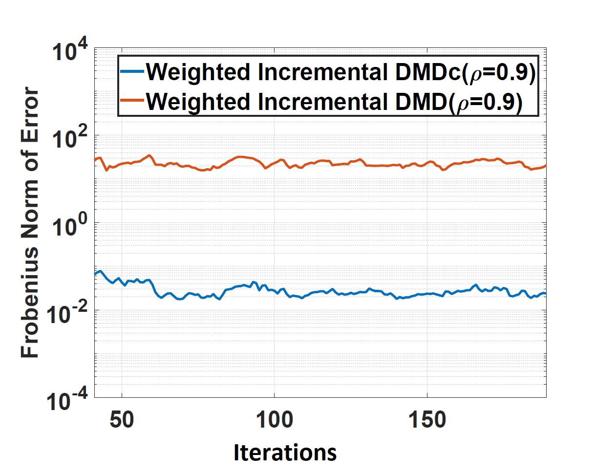
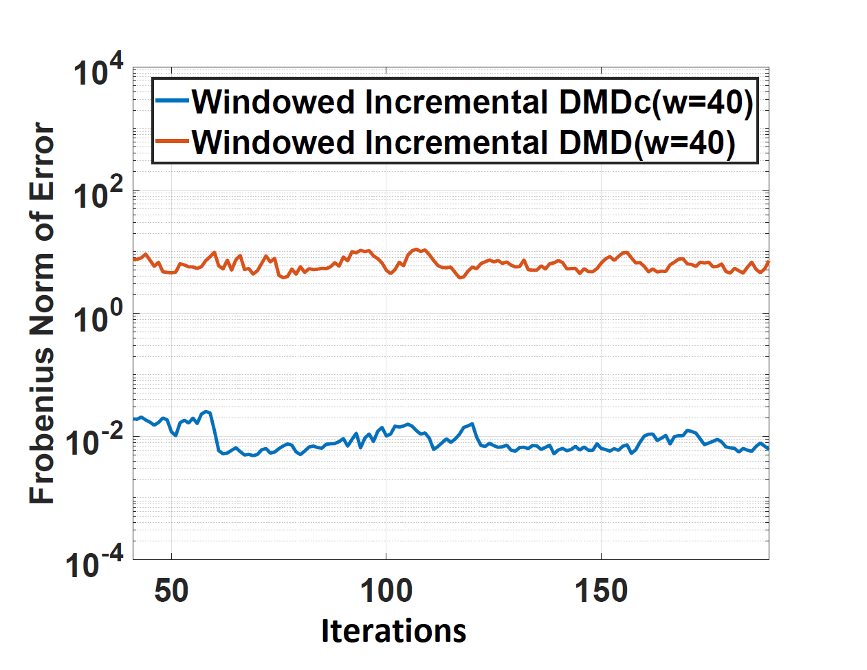
Refer to caption
(a) Weighted Incremental DMDc
Refer to caption
(b) Windowed Incremental DMDc
Fig. 12: The Frobenius norm of prediction error for a future-window of 10 samples using (a) weighted incremental DMD (red line) and weighted incremental DMDc(blue line), and (b) windowed incremental DMD (red line) and windowed incremental DMDc (blue line).

7 Conclusion and Future Direction

In this paper, we developed algorithms for incremental computation of time-varying dynamic mode decomposition for autonomous and non-autonomous systems. In contrast to existing algorithms, these algorithms rely on incremental singular value decomposition to update singular values of the data matrix and allow for computation of a reduced order model at each time step. These algorithms are particularly useful for the cases in which the data matrix is singular and incremental matrix inversion based algorithms cannot be applied. We applied the proposed algorithms to an EEG dataset associated with error-related potentials and showed the efficacy of the algorithms in terms of predicting the future EEG signal. We also illustrated that the principal DMD modes obtained were consistent with the EEG activity seen in the brain.

There are several interesting future research directions for this work. First, the proposed approach can be adapted to apply the incremental updates on a nonlinear mapping of the measurements. This could be done in the spirit of extended dynamic mode decomposition proposed in [34]. Such extension may further improve the predictive power of the computed models. Second, it would be interesting to conduct human-in-the-loop experiments in which the EEG data is used in real-time to computed a DMD-based model of human performance and the control is designed to improve the performance.

Code

The MATLAB code used to generate the numerical results presented in this paper is available at
https://github.com/MSU-dcypherlab/Incremental-DMD-for-EEG-Data.git.

Appendix A Proof of Proposition 1

The incremented dataset 𝐗k+1subscript𝐗𝑘1\mathbf{X}_{k+1} can be represented in term of 𝐗ksubscript𝐗𝑘\mathbf{X}_{k} using the following additive updating formula

𝐗k+1subscript𝐗𝑘1\displaystyle\mathbf{X}_{k+1} =ρ[𝐗k𝟎]+𝐱k+1𝐳k+1T,absent𝜌matrixsubscript𝐗𝑘0subscript𝐱𝑘1superscriptsubscript𝐳𝑘1T\displaystyle=\rho\begin{bmatrix}\mathbf{X}_{k}&\mathbf{0}\end{bmatrix}+\mathbf{x}_{k+1}\mathbf{z}_{k+1}^{\text{T}},
=ρ𝐔xk𝚺xk[𝐕xk𝟎]+𝐱k+1𝐳k+1Tabsent𝜌subscript𝐔subscript𝑥𝑘subscript𝚺subscript𝑥𝑘matrixsubscriptsuperscript𝐕subscript𝑥𝑘0subscript𝐱𝑘1superscriptsubscript𝐳𝑘1T\displaystyle=\rho\mathbf{U}_{x_{k}}\mathbf{\Sigma}_{x_{k}}\begin{bmatrix}\mathbf{V}^{*}_{x_{k}}&\mathbf{0}\end{bmatrix}+\mathbf{x}_{k+1}\mathbf{z}_{k+1}^{\text{T}}
=[ρ𝐔xk𝐱k+1][𝚺k𝟎𝟎1][[𝐕k𝟎]𝐳k+1]absentmatrix𝜌subscript𝐔subscript𝑥𝑘subscript𝐱𝑘1matrixsubscript𝚺𝑘001superscriptmatrixmatrixsubscript𝐕𝑘0subscript𝐳𝑘1\displaystyle=\begin{bmatrix}\rho\mathbf{U}_{x_{k}}&\mathbf{x}_{k+1}\end{bmatrix}\begin{bmatrix}\mathbf{\Sigma}_{k}&\mathbf{0}\\ \mathbf{0}&1\end{bmatrix}\begin{bmatrix}\begin{bmatrix}\mathbf{V}_{k}\\ \mathbf{0}\end{bmatrix}&\mathbf{z}_{k+1}\end{bmatrix}^{\ast}
=ρ𝐔xk[𝐈ρ1𝐔xk𝐱k+1][𝚺k𝟎𝟎1][𝐕k𝟎𝟎1]absent𝜌subscript𝐔subscript𝑥𝑘matrix𝐈superscript𝜌1superscriptsubscript𝐔subscript𝑥𝑘subscript𝐱𝑘1matrixsubscript𝚺𝑘001superscriptmatrixsubscript𝐕𝑘001\displaystyle=\rho\mathbf{U}_{x_{k}}\begin{bmatrix}\mathbf{I}&\rho^{-1}\mathbf{U}_{x_{k}}^{*}\mathbf{x}_{k+1}\end{bmatrix}\begin{bmatrix}\mathbf{\Sigma}_{k}&\mathbf{0}\\ \mathbf{0}&1\end{bmatrix}\begin{bmatrix}\mathbf{{V}}_{k}&\mathbf{0}\\ \mathbf{0}&1\end{bmatrix}^{\ast}
=ρ𝐔xk[𝚺xkρ1𝐔xk𝐱k+1][𝐕xk𝟎𝟎1].absent𝜌subscript𝐔subscript𝑥𝑘matrixsubscript𝚺subscript𝑥𝑘superscript𝜌1superscriptsubscript𝐔subscript𝑥𝑘subscript𝐱𝑘1superscriptmatrixsubscript𝐕subscript𝑥𝑘001\displaystyle=\rho\mathbf{U}_{x_{k}}\begin{bmatrix}\mathbf{\Sigma}_{x_{k}}&\rho^{-1}\mathbf{U}_{x_{k}}^{*}\mathbf{x}_{k+1}\end{bmatrix}\begin{bmatrix}\mathbf{{V}}_{x_{k}}&\mathbf{0}\\ \mathbf{0}&1\end{bmatrix}^{\ast}. (48)

where 𝐳k+1=[001]Tk+1subscript𝐳𝑘1superscriptmatrix001Tsuperscript𝑘1\mathbf{z}_{k+1}=\begin{bmatrix}0&0&\cdots&1\end{bmatrix}^{\text{T}}\in\mathbb{R}^{k+1}.

Let the SVD of 𝐒k[𝚺xkρ1𝐔xk𝐱k+1]=𝐔sk𝚺sk𝐕sksubscript𝐒𝑘matrixsubscript𝚺subscript𝑥𝑘superscript𝜌1superscriptsubscript𝐔subscript𝑥𝑘subscript𝐱𝑘1subscript𝐔subscript𝑠𝑘subscript𝚺subscript𝑠𝑘subscriptsuperscript𝐕subscript𝑠𝑘\mathbf{S}_{k}\triangleq\begin{bmatrix}\mathbf{\Sigma}_{x_{k}}&\rho^{-1}\mathbf{U}_{x_{k}}^{*}\mathbf{x}_{k+1}\end{bmatrix}=\mathbf{U}_{s_{k}}\mathbf{\Sigma}_{s_{k}}\mathbf{V}^{*}_{s_{k}} with 𝐔skn×nsubscript𝐔subscript𝑠𝑘superscript𝑛𝑛\mathbf{U}_{s_{k}}\in\mathbb{C}^{n\times n}, 𝚺skn×nsubscript𝚺subscript𝑠𝑘superscript𝑛𝑛\mathbf{\Sigma}_{s_{k}}\in\mathbb{C}^{n\times n}, and 𝐕sk(n+1)×nsubscript𝐕subscript𝑠𝑘superscript𝑛1𝑛\mathbf{V}_{s_{k}}\in\mathbb{C}^{(n+1)\times n}. Then, 𝐕sksubscript𝐕subscript𝑠𝑘\mathbf{V}_{s_{k}} can be partitioned as 𝐕sk=[𝐕sk,1𝐯sk,2]subscript𝐕subscript𝑠𝑘matrixsubscript𝐕subscript𝑠𝑘1subscript𝐯subscript𝑠𝑘2\mathbf{V}_{s_{k}}=\begin{bmatrix}\mathbf{V}_{s_{k,1}}\\ \mathbf{v}_{s_{k,2}}\end{bmatrix} such that 𝐯sk,21×nsubscript𝐯subscript𝑠𝑘2superscript1𝑛\mathbf{v}_{s_{k,2}}\in\mathbb{C}^{1\times n} is orthogonal to 𝐕sk,1n×nsubscript𝐕subscript𝑠𝑘1superscript𝑛𝑛\mathbf{V}_{s_{k,1}}\in\mathbb{C}^{n\times n}, and 𝐗k+1subscript𝐗𝑘1\mathbf{X}_{k+1} in (22) can be written as:

𝐗k+1=ρ𝐔xk𝐔sk𝚺sk[𝐕xk𝐕sk,1𝐯sk,2].subscript𝐗𝑘1𝜌subscript𝐔subscript𝑥𝑘subscript𝐔subscript𝑠𝑘subscript𝚺subscript𝑠𝑘superscriptmatrixsubscript𝐕subscript𝑥𝑘subscript𝐕subscript𝑠𝑘1subscript𝐯subscript𝑠𝑘2\mathbf{X}_{k+1}=\rho\mathbf{U}_{x_{k}}\mathbf{U}_{s_{k}}\mathbf{\Sigma}_{s_{k}}\begin{bmatrix}\mathbf{V}_{x_{k}}\mathbf{V}_{s_{k,1}}\\ \mathbf{v}_{s_{k,2}}\end{bmatrix}^{\ast}.

Thus, the SVD of 𝐗k+1=𝐔xk+1𝚺xk+1𝐕xk+1subscript𝐗𝑘1subscript𝐔subscript𝑥𝑘1subscript𝚺subscript𝑥𝑘1subscriptsuperscript𝐕subscript𝑥𝑘1\mathbf{X}_{k+1}=\mathbf{U}_{x_{k+1}}\mathbf{\Sigma}_{x_{k+1}}\mathbf{V}^{*}_{x_{k+1}} is given by

𝐔xk+1=𝐔xk𝐔sk,𝚺k+1=ρ𝚺sk,and𝐕xk+1=[𝐕xk𝐕sk,1𝐯sk,2].formulae-sequencesubscript𝐔subscript𝑥𝑘1subscript𝐔subscript𝑥𝑘subscript𝐔subscript𝑠𝑘formulae-sequencesubscript𝚺𝑘1𝜌subscript𝚺subscript𝑠𝑘andsubscript𝐕subscript𝑥𝑘1matrixsubscript𝐕subscript𝑥𝑘subscript𝐕subscript𝑠𝑘1subscript𝐯subscript𝑠𝑘2\displaystyle\mathbf{U}_{x_{k+1}}=\mathbf{U}_{x_{k}}\mathbf{U}_{s_{k}},~{}\mathbf{\Sigma}_{k+1}=\rho\mathbf{\Sigma}_{s_{k}},~{}\text{and}~{}\mathbf{V}_{x_{k+1}}=\begin{bmatrix}\mathbf{V}_{x_{k}}\mathbf{V}_{s_{k,1}}\\ \mathbf{v}_{s_{k,2}}\end{bmatrix}.

Appendix B Proof of Proposition 2

Consider the updated dataset

𝝌~´ksubscriptbold-´bold-~𝝌𝑘\displaystyle\boldsymbol{\acute{\tilde{\chi}}}_{k} =𝝌k𝐱kw+1𝐳1Tabsentsubscript𝝌𝑘subscript𝐱𝑘𝑤1superscriptsubscript𝐳1T\displaystyle=\boldsymbol{\chi}_{k}-\mathbf{x}_{k-w+1}\mathbf{z}_{1}^{\text{T}}
=𝐔χk𝐔χk(𝝌k𝐱kw+1𝐳1T)𝐕χk𝐕χkabsentsubscript𝐔subscript𝜒𝑘superscriptsubscript𝐔subscript𝜒𝑘subscript𝝌𝑘subscript𝐱𝑘𝑤1superscriptsubscript𝐳1Tsubscript𝐕subscript𝜒𝑘superscriptsubscript𝐕subscript𝜒𝑘\displaystyle=\mathbf{U}_{\chi_{k}}\mathbf{U}_{\chi_{k}}^{*}(\boldsymbol{\chi}_{k}-\mathbf{x}_{k-w+1}\mathbf{z}_{1}^{\text{T}})\mathbf{V}_{\chi_{k}}\mathbf{V}_{\chi_{k}}^{*}
=𝐔χk(𝚺χk𝐔χk𝐱kw+1𝐳1T𝐕χk)𝐕χk,absentsubscript𝐔subscript𝜒𝑘subscript𝚺subscript𝜒𝑘superscriptsubscript𝐔subscript𝜒𝑘subscript𝐱𝑘𝑤1superscriptsubscript𝐳1Tsubscript𝐕subscript𝜒𝑘superscriptsubscript𝐕subscript𝜒𝑘\displaystyle=\mathbf{U}_{\chi_{k}}(\mathbf{\Sigma}_{\chi_{k}}-\mathbf{U}_{\chi_{k}}^{*}\mathbf{x}_{k-w+1}\mathbf{z}_{1}^{\text{T}}\mathbf{V}_{\chi_{k}})\mathbf{V}_{\chi_{k}}^{*}, (49)

where 𝝌~´k[0𝐱kw+2𝐱k]subscriptbold-´bold-~𝝌𝑘matrix0subscript𝐱𝑘𝑤2subscript𝐱𝑘\boldsymbol{\acute{\tilde{\chi}}}_{k}\triangleq\begin{bmatrix}0&\mathbf{x}_{k-w+2}&\cdots&\mathbf{x}_{k}\end{bmatrix} is the 𝝌´ksubscriptbold-´𝝌𝑘\boldsymbol{\acute{\chi}}_{k} dataset padded with n𝑛n-dimensional zero column, and 𝐳1=[100]Twsubscript𝐳1superscriptmatrix100Tsuperscript𝑤\mathbf{z}_{1}=\begin{bmatrix}1&0&\cdots&0\end{bmatrix}^{\text{T}}\in\mathbb{R}^{w}.

Let the SVD of 𝐒´k𝚺χk𝐔χk𝐱kw+1𝐳1T𝐕χksubscript´𝐒𝑘subscript𝚺subscript𝜒𝑘superscriptsubscript𝐔subscript𝜒𝑘subscript𝐱𝑘𝑤1superscriptsubscript𝐳1Tsubscript𝐕subscript𝜒𝑘\mathbf{\acute{S}}_{k}\triangleq\mathbf{\Sigma}_{\chi_{k}}-\mathbf{U}_{\chi_{k}}^{*}\mathbf{x}_{k-w+1}\mathbf{z}_{1}^{\text{T}}\mathbf{V}_{\chi_{k}} be

𝐒´k=𝐔s´k[𝚺s´k𝟎q×(wq)][𝐕s´k𝐕~s´k],subscript´𝐒𝑘subscript𝐔subscript´𝑠𝑘matrixsubscript𝚺subscript´𝑠𝑘subscript0𝑞𝑤𝑞superscriptmatrixsubscript𝐕subscript´𝑠𝑘subscript~𝐕subscript´𝑠𝑘\mathbf{\acute{S}}_{k}=\mathbf{U}_{\acute{s}_{k}}\begin{bmatrix}{\mathbf{\Sigma}}_{\acute{s}_{k}}&\mathbf{0}_{q\times(w-q)}\end{bmatrix}\begin{bmatrix}\mathbf{V}_{\acute{s}_{k}}&\tilde{\mathbf{V}}_{\acute{s}_{k}}\end{bmatrix}^{\ast}, (50)

where 𝐔s´kq×qsubscript𝐔subscript´𝑠𝑘superscript𝑞𝑞\mathbf{U}_{\acute{s}_{k}}\in\mathbb{C}^{q\times q}, 𝚺s´kq×qsubscript𝚺subscript´𝑠𝑘superscript𝑞𝑞{\mathbf{\Sigma}}_{\acute{s}_{k}}\in\mathbb{C}^{q\times q}, 𝐕s´kw×qsubscript𝐕subscript´𝑠𝑘superscript𝑤𝑞\mathbf{V}_{\acute{s}_{k}}\in\mathbb{C}^{w\times q} and 𝐕~s´kw×(wq)subscript~𝐕subscript´𝑠𝑘superscript𝑤𝑤𝑞\tilde{\mathbf{V}}_{\acute{s}_{k}}\in\mathbb{C}^{w\times(w-q)}. Let 𝐕χksubscript𝐕subscript𝜒𝑘\mathbf{V}_{\chi_{k}} be partitioned into 𝐕χk=[𝐯χk,1𝐕χk,2]subscript𝐕subscript𝜒𝑘matrixsubscript𝐯subscript𝜒𝑘1subscript𝐕subscript𝜒𝑘2\mathbf{V}_{\chi_{k}}=\begin{bmatrix}\mathbf{v}_{\chi_{k,1}}\\ \mathbf{V}_{\chi_{k,2}}\end{bmatrix}, where 𝐯χk,11×wsubscript𝐯subscript𝜒𝑘1superscript1𝑤\mathbf{v}_{\chi_{k,1}}\in\mathbb{C}^{1\times w} and 𝐕χk,2(w1)×wsubscript𝐕subscript𝜒𝑘2superscript𝑤1𝑤\mathbf{V}_{\chi_{k,2}}\in\mathbb{C}^{(w-1)\times w}.

Substituting the SVD from equation (50) into equation(49), the dataset 𝐗~´ksubscript´~𝐗𝑘\mathbf{\acute{{\tilde{X}}}}_{k} can be expressed as:

𝝌~´ksubscriptbold-´bold-~𝝌𝑘\displaystyle\boldsymbol{\acute{\tilde{\chi}}}_{k} =(𝐔χk𝐔s´k)[𝚺s´k𝟎q×(wq)](𝐕χk[𝐕s´k𝐕~s´k])absentsubscript𝐔subscript𝜒𝑘subscript𝐔subscript´𝑠𝑘matrixsubscript𝚺subscript´𝑠𝑘subscript0𝑞𝑤𝑞superscriptsubscript𝐕subscript𝜒𝑘matrixsubscript𝐕subscript´𝑠𝑘subscript~𝐕subscript´𝑠𝑘\displaystyle=\left(\mathbf{U}_{\chi_{k}}\mathbf{U}_{\acute{s}_{k}}\right)\begin{bmatrix}{\mathbf{\Sigma}}_{\acute{s}_{k}}&\mathbf{0}_{q\times(w-q)}\end{bmatrix}\left(\mathbf{V}_{\chi_{k}}\begin{bmatrix}\mathbf{V}_{\acute{s}_{k}}&\tilde{\mathbf{V}}_{\acute{s}_{k}}\end{bmatrix}\right)^{\ast}
=(𝐔χk𝐔s´k)[𝚺s´k𝟎q×(wq)]([𝐯χk,1𝐕χk,2][𝐕s´k𝐕~s´k])absentsubscript𝐔subscript𝜒𝑘subscript𝐔subscript´𝑠𝑘matrixsubscript𝚺subscript´𝑠𝑘subscript0𝑞𝑤𝑞superscriptmatrixsubscript𝐯subscript𝜒𝑘1subscript𝐕subscript𝜒𝑘2matrixsubscript𝐕subscript´𝑠𝑘subscript~𝐕subscript´𝑠𝑘\displaystyle=\left(\mathbf{U}_{\chi_{k}}\mathbf{U}_{\acute{s}_{k}}\right)\begin{bmatrix}{\mathbf{\Sigma}}_{\acute{s}_{k}}&\mathbf{0}_{q\times(w-q)}\end{bmatrix}\left(\begin{bmatrix}\mathbf{v}_{\chi_{k,1}}\\ \mathbf{V}_{\chi_{k,2}}\end{bmatrix}\begin{bmatrix}\mathbf{V}_{\acute{s}_{k}}&\tilde{\mathbf{V}}_{\acute{s}_{k}}\end{bmatrix}\right)^{\ast}
=(𝐔χk𝐔s´k)[𝚺s´k𝟎q×(wq)][𝐯χk,1𝐕s´k𝐯χk,1𝐕~s´k𝐕χk,2𝐕s´k𝐕χk,2𝐕~s´k]absentsubscript𝐔subscript𝜒𝑘subscript𝐔subscript´𝑠𝑘matrixsubscript𝚺subscript´𝑠𝑘subscript0𝑞𝑤𝑞superscriptmatrixsubscript𝐯subscript𝜒𝑘1subscript𝐕subscript´𝑠𝑘subscript𝐯subscript𝜒𝑘1subscript~𝐕subscript´𝑠𝑘subscript𝐕subscript𝜒𝑘2subscript𝐕subscript´𝑠𝑘subscript𝐕subscript𝜒𝑘2subscript~𝐕subscript´𝑠𝑘\displaystyle=\left(\mathbf{U}_{\chi_{k}}\mathbf{U}_{\acute{s}_{k}}\right)\begin{bmatrix}{\mathbf{\Sigma}}_{\acute{s}_{k}}&\mathbf{0}_{q\times(w-q)}\end{bmatrix}\begin{bmatrix}\mathbf{v}_{\chi_{k,1}}\mathbf{V}_{\acute{s}_{k}}&\mathbf{v}_{\chi_{k,1}}\tilde{\mathbf{V}}_{\acute{s}_{k}}\\ \mathbf{V}_{\chi_{k,2}}\mathbf{V}_{\acute{s}_{k}}&\mathbf{V}_{\chi_{k,2}}\tilde{\mathbf{V}}_{\acute{s}_{k}}\end{bmatrix}^{\ast}
=[𝐔χk𝐔s´k𝚺s´k𝐕s´k𝐯χk,1𝐔χk𝐔s´k𝚺s´k𝐕s´k𝐕χk,2].absentmatrixsubscript𝐔subscript𝜒𝑘subscript𝐔subscript´𝑠𝑘subscript𝚺subscript´𝑠𝑘superscriptsubscript𝐕subscript´𝑠𝑘superscriptsubscript𝐯subscript𝜒𝑘1subscript𝐔subscript𝜒𝑘subscript𝐔subscript´𝑠𝑘subscript𝚺subscript´𝑠𝑘superscriptsubscript𝐕subscript´𝑠𝑘superscriptsubscript𝐕subscript𝜒𝑘2\displaystyle=\begin{bmatrix}\mathbf{U}_{\chi_{k}}\mathbf{U}_{\acute{s}_{k}}{\mathbf{\Sigma}}_{\acute{s}_{k}}\mathbf{V}_{\acute{s}_{k}}^{*}\mathbf{v}_{\chi_{k,1}}^{*}&\mathbf{U}_{\chi_{k}}\mathbf{U}_{\acute{s}_{k}}{\mathbf{\Sigma}}_{\acute{s}_{k}}\mathbf{V}_{\acute{s}_{k}}^{*}\mathbf{V}_{\chi_{k,2}}^{*}\end{bmatrix}.

Since, 𝝌~´k=[𝟎𝝌´k]subscriptbold-´bold-~𝝌𝑘matrix0subscriptbold-´𝝌𝑘\boldsymbol{\acute{\tilde{\chi}}}_{k}=\begin{bmatrix}\mathbf{0}&\boldsymbol{\acute{{\chi}}}_{k}\end{bmatrix}, it follows that 𝐔χk𝐔s´k𝚺s´k𝐕s´k𝐯χk,1=𝟎subscript𝐔subscript𝜒𝑘subscript𝐔subscript´𝑠𝑘subscript𝚺subscript´𝑠𝑘superscriptsubscript𝐕subscript´𝑠𝑘superscriptsubscript𝐯subscript𝜒𝑘10\mathbf{U}_{\chi_{k}}\mathbf{U}_{\acute{s}_{k}}{\mathbf{\Sigma}}_{\acute{s}_{k}}\mathbf{V}_{\acute{s}_{k}}^{*}\mathbf{v}_{\chi_{k,1}}^{*}=\mathbf{0} and 𝝌´k=𝐔χk𝐔s´k𝚺s´k𝐕s´k𝐕χk,2subscriptbold-´𝝌𝑘subscript𝐔subscript𝜒𝑘subscript𝐔subscript´𝑠𝑘subscript𝚺subscript´𝑠𝑘superscriptsubscript𝐕subscript´𝑠𝑘superscriptsubscript𝐕subscript𝜒𝑘2\boldsymbol{\acute{{\chi}}}_{k}=\mathbf{U}_{\chi_{k}}\mathbf{U}_{\acute{s}_{k}}{\mathbf{\Sigma}}_{\acute{s}_{k}}\mathbf{V}_{\acute{s}_{k}}^{*}\mathbf{V}_{\chi_{k,2}}^{*}. Thus, the SVD of 𝝌´k=𝐔χ´k𝚺χ´k𝐕χ´ksubscriptbold-´𝝌𝑘subscript𝐔subscript´𝜒𝑘subscript𝚺subscript´𝜒𝑘superscriptsubscript𝐕subscript´𝜒𝑘\boldsymbol{\acute{\chi}}_{k}=\mathbf{U}_{\acute{\chi}_{k}}{\mathbf{\Sigma}}_{\acute{\chi}_{k}}{\mathbf{V}}_{\acute{\chi}_{k}}^{*} is

𝐔χ´k=𝐔χk𝐔s´k,𝚺χ´k=𝚺s´k,and𝐕χ´k=𝐕χk,2𝐕s´k.formulae-sequencesubscript𝐔subscript´𝜒𝑘subscript𝐔subscript𝜒𝑘subscript𝐔subscript´𝑠𝑘formulae-sequencesubscript𝚺subscript´𝜒𝑘subscript𝚺subscript´𝑠𝑘andsubscript𝐕subscript´𝜒𝑘subscript𝐕subscript𝜒𝑘2subscript𝐕subscript´𝑠𝑘\displaystyle\mathbf{U}_{\acute{\chi}_{k}}=\mathbf{U}_{\chi_{k}}\mathbf{U}_{\acute{s}_{k}},~{}{\mathbf{\Sigma}}_{\acute{\chi}_{k}}={\mathbf{\Sigma}}_{\acute{s}_{k}},~{}\text{and}~{}{\mathbf{V}}_{\acute{\chi}_{k}}=\mathbf{V}_{\chi_{k,2}}\mathbf{V}_{\acute{s}_{k}}. (51)

A noteworthy property of the above decomposition that we will use in the later developments is that 𝐯χk,1𝐕s´k=𝟎subscript𝐯subscript𝜒𝑘1subscript𝐕subscript´𝑠𝑘0\mathbf{v}_{\chi_{k,1}}\mathbf{V}_{\acute{s}_{k}}=\mathbf{0}. To establish this property, we note that since 𝐔χk𝐒´k𝐯χk,1=𝟎subscript𝐔subscript𝜒𝑘subscript´𝐒𝑘superscriptsubscript𝐯subscript𝜒𝑘10\mathbf{U}_{\chi_{k}}\mathbf{\acute{S}}_{k}\mathbf{v}_{\chi_{k,1}}^{*}=\mathbf{0}, 𝐯χk,1Ker(𝐔χk𝐒´k)subscriptsuperscript𝐯subscript𝜒𝑘1Kersubscript𝐔subscript𝜒𝑘subscript´𝐒𝑘\mathbf{v}^{*}_{\chi_{k,1}}\in\text{Ker}(\mathbf{U}_{\chi_{k}}\mathbf{\acute{S}}_{k}). Furthermore, since 𝐔χksubscript𝐔subscript𝜒𝑘\mathbf{U}_{\chi_{k}} is full rank, then 𝐯χk,1Ker(𝐒´k)=span(𝐕~s´k)subscriptsuperscript𝐯subscript𝜒𝑘1Kersubscript´𝐒𝑘spansubscript~𝐕subscript´𝑠𝑘\mathbf{v}^{*}_{\chi_{k,1}}\in\text{Ker}(\mathbf{\acute{S}}_{k})=\text{span}(\tilde{\mathbf{V}}_{\acute{s}_{k}}), and consequently

𝐯χk,1𝐕s´k=𝟎.subscript𝐯subscript𝜒𝑘1subscript𝐕subscript´𝑠𝑘0\displaystyle\mathbf{v}_{\chi_{k,1}}\mathbf{V}_{\acute{s}_{k}}=\mathbf{0}. (52)

Appendix C Proof of Theorem 1

Let the SVD of 𝐗k+1=𝐔xk+1𝚺xk+1𝐕xk+1subscript𝐗𝑘1subscript𝐔subscript𝑥𝑘1subscript𝚺subscript𝑥𝑘1subscriptsuperscript𝐕subscript𝑥𝑘1\mathbf{X}_{k+1}=\mathbf{U}_{x_{k+1}}{\mathbf{\Sigma}_{x_{k+1}}}\mathbf{V}^{*}_{x_{k+1}} be calculated by the incremental SVD update (23). Then, the time-varying DMD operator (15) at sampling time tk+1subscript𝑡𝑘1t_{k+1} is:

𝐀k+1ρsubscriptsuperscript𝐀𝜌𝑘1\displaystyle\mathbf{A}^{\rho}_{k+1} =\displaystyle= 𝐘k+1𝐕xk+1𝚺xk+11𝐔xk+1subscript𝐘𝑘1subscript𝐕subscript𝑥𝑘1superscriptsubscript𝚺subscript𝑥𝑘11superscriptsubscript𝐔subscript𝑥𝑘1\displaystyle\mathbf{Y}_{k+1}\mathbf{V}_{x_{k+1}}{\mathbf{\Sigma}_{x_{k+1}}^{-1}}\mathbf{U}_{x_{k+1}}^{*} (53)
=\displaystyle= [ρ𝐘k𝐲k+1]𝐕xk+1𝚺xk+11𝐔xk+1.matrix𝜌subscript𝐘𝑘subscript𝐲𝑘1subscript𝐕subscript𝑥𝑘1superscriptsubscript𝚺subscript𝑥𝑘11superscriptsubscript𝐔subscript𝑥𝑘1\displaystyle\begin{bmatrix}\rho\mathbf{Y}_{k}&\mathbf{y}_{k+1}\end{bmatrix}\mathbf{V}_{x_{k+1}}{\mathbf{\Sigma}_{x_{k+1}}^{-1}}\mathbf{U}_{x_{k+1}}^{*}.

Substituting the incrementally computed 𝐕k+1subscript𝐕𝑘1\mathbf{V}_{k+1} from (23) into the DMD operator (53) yields:

𝐀k+1ρ=subscriptsuperscript𝐀𝜌𝑘1absent\displaystyle\mathbf{A}^{\rho}_{k+1}= [ρ𝐘k𝐲k+1][𝐕xk𝐕sk,1𝐯sk,2]𝚺xk+11𝐔xk+1matrix𝜌subscript𝐘𝑘subscript𝐲𝑘1matrixsubscript𝐕subscript𝑥𝑘subscript𝐕subscript𝑠𝑘1subscript𝐯subscript𝑠𝑘2superscriptsubscript𝚺subscript𝑥𝑘11superscriptsubscript𝐔subscript𝑥𝑘1\displaystyle\begin{bmatrix}\rho\mathbf{Y}_{k}&\mathbf{y}_{k+1}\end{bmatrix}\begin{bmatrix}\mathbf{V}_{x_{k}}\mathbf{V}_{s_{k,1}}\\ \mathbf{v}_{s_{k,2}}\end{bmatrix}\mathbf{\Sigma}_{x_{k+1}}^{-1}\mathbf{U}_{x_{k+1}}^{*}
=\displaystyle= (ρ𝐘k𝐕xk𝐕sk,1+𝐲k+1𝐯sk,2)𝚺xk+11𝐔xk+1𝜌subscript𝐘𝑘subscript𝐕subscript𝑥𝑘subscript𝐕subscript𝑠𝑘1subscript𝐲𝑘1subscript𝐯subscript𝑠𝑘2superscriptsubscript𝚺subscript𝑥𝑘11subscriptsuperscript𝐔subscript𝑥𝑘1\displaystyle\left(\rho\mathbf{Y}_{k}\mathbf{V}_{x_{k}}\mathbf{V}_{s_{k,1}}+\mathbf{y}_{k+1}\mathbf{v}_{s_{k,2}}\right)\mathbf{\Sigma}_{x_{k+1}}^{-1}\mathbf{U}^{*}_{x_{k+1}}
=\displaystyle= (ρ𝐘k𝐕xk(𝚺xk1ρ1𝐔xkρ𝐔xk𝚺xk)=In𝐕sk,1+𝐲k+1𝐯sk,2)𝚺xk+11𝐔xk+1𝜌subscript𝐘𝑘subscript𝐕subscript𝑥𝑘absentsubscript𝐼𝑛superscriptsubscript𝚺subscript𝑥𝑘1superscript𝜌1subscriptsuperscript𝐔subscript𝑥𝑘𝜌subscript𝐔subscript𝑥𝑘subscript𝚺subscript𝑥𝑘subscript𝐕subscript𝑠𝑘1subscript𝐲𝑘1subscript𝐯subscript𝑠𝑘2superscriptsubscript𝚺subscript𝑥𝑘11subscriptsuperscript𝐔subscript𝑥𝑘1\displaystyle\Big{(}\rho\mathbf{Y}_{k}\mathbf{V}_{x_{k}}\underset{=I_{n}}{\underbrace{(\mathbf{\Sigma}_{x_{k}}^{-1}\rho^{-1}\mathbf{U}^{*}_{x_{k}}\rho\mathbf{U}_{x_{k}}\mathbf{\Sigma}_{x_{k}})}}\mathbf{V}_{s_{k,1}}+\mathbf{y}_{k+1}\mathbf{v}_{s_{k,2}}\Big{)}\mathbf{\Sigma}_{x_{k+1}}^{-1}\mathbf{U}^{*}_{x_{k+1}}
=\displaystyle= (𝐀kρρ𝐔xk𝚺xk𝐕sk,1+𝐲k+1𝐯sk,2)𝚺xk+11𝐔xk+1subscriptsuperscript𝐀𝜌𝑘𝜌subscript𝐔subscript𝑥𝑘subscript𝚺subscript𝑥𝑘subscript𝐕subscript𝑠𝑘1subscript𝐲𝑘1subscript𝐯subscript𝑠𝑘2superscriptsubscript𝚺subscript𝑥𝑘11subscriptsuperscript𝐔subscript𝑥𝑘1\displaystyle\left(\mathbf{A}^{\rho}_{k}\rho\mathbf{U}_{x_{k}}\mathbf{\Sigma}_{x_{k}}\mathbf{V}_{s_{k,1}}+\mathbf{y}_{k+1}\mathbf{v}_{s_{k,2}}\right)\mathbf{\Sigma}_{x_{k+1}}^{-1}\mathbf{U}^{*}_{x_{k+1}}
=\displaystyle= 𝐀kρ𝐀kρ+(𝐀kρρ𝐔xk𝚺xk𝐕sk,1+𝐲k+1𝐯sk,1)𝚺xk+11𝐔xk+1subscriptsuperscript𝐀𝜌𝑘subscriptsuperscript𝐀𝜌𝑘subscriptsuperscript𝐀𝜌𝑘𝜌subscript𝐔subscript𝑥𝑘subscript𝚺subscript𝑥𝑘subscript𝐕subscript𝑠𝑘1subscript𝐲𝑘1subscript𝐯subscript𝑠𝑘1superscriptsubscript𝚺subscript𝑥𝑘11subscriptsuperscript𝐔subscript𝑥𝑘1\displaystyle\mathbf{A}^{\rho}_{k}-\mathbf{A}^{\rho}_{k}+\left(\mathbf{A}^{\rho}_{k}\rho\mathbf{U}_{x_{k}}\mathbf{\Sigma}_{x_{k}}\mathbf{V}_{s_{k,1}}+\mathbf{y}_{k+1}\mathbf{v}_{s_{k,1}}\right)\mathbf{\Sigma}_{x_{k+1}}^{-1}\mathbf{U}^{*}_{x_{k+1}} (54)
=\displaystyle= 𝐀kρ𝐀kρ(𝐔xk+1𝚺xk+1𝚺xk+11𝐔xk+1)=In+𝐀kρρ𝐔xk𝚺xk𝐕sk,1𝚺xk+11𝐔xk+1+𝐲k+1𝐯sk,2𝚺xk+11𝐔xk+1subscriptsuperscript𝐀𝜌𝑘subscriptsuperscript𝐀𝜌𝑘absentsubscript𝐼𝑛subscript𝐔subscript𝑥𝑘1subscript𝚺subscript𝑥𝑘1superscriptsubscript𝚺subscript𝑥𝑘11subscriptsuperscript𝐔subscript𝑥𝑘1subscriptsuperscript𝐀𝜌𝑘𝜌subscript𝐔subscript𝑥𝑘subscript𝚺subscript𝑥𝑘subscript𝐕subscript𝑠𝑘1superscriptsubscript𝚺subscript𝑥𝑘11subscriptsuperscript𝐔subscript𝑥𝑘1subscript𝐲𝑘1subscript𝐯subscript𝑠𝑘2superscriptsubscript𝚺subscript𝑥𝑘11subscriptsuperscript𝐔subscript𝑥𝑘1\displaystyle\mathbf{A}^{\rho}_{k}-\mathbf{A}^{\rho}_{k}\underset{=I_{n}}{\underbrace{(\mathbf{U}_{x_{k+1}}\mathbf{\Sigma}_{x_{k+1}}\mathbf{\Sigma}_{x_{k+1}}^{-1}\mathbf{U}^{*}_{x_{k+1}})}}+\mathbf{A}^{\rho}_{k}\rho\mathbf{U}_{x_{k}}\mathbf{\Sigma}_{x_{k}}\mathbf{V}_{s_{k,1}}\mathbf{\Sigma}_{x_{k+1}}^{-1}\mathbf{U}^{*}_{x_{k+1}}+\mathbf{y}_{k+1}\mathbf{v}_{s_{k,2}}\mathbf{\Sigma}_{x_{k+1}}^{-1}\mathbf{U}^{*}_{x_{k+1}}
=\displaystyle= 𝐀kρ+𝐲k+1𝐯sk,2𝚺xk+11𝐔xk+1𝐀kρ(𝐔xk+1𝚺xk+1ρ𝐔xk𝚺xk𝐕sk,1)𝚺xk+11𝐔xk+1,subscriptsuperscript𝐀𝜌𝑘subscript𝐲𝑘1subscript𝐯subscript𝑠𝑘2superscriptsubscript𝚺subscript𝑥𝑘11subscriptsuperscript𝐔subscript𝑥𝑘1subscriptsuperscript𝐀𝜌𝑘subscript𝐔subscript𝑥𝑘1subscript𝚺subscript𝑥𝑘1𝜌subscript𝐔subscript𝑥𝑘subscript𝚺subscript𝑥𝑘subscript𝐕subscript𝑠𝑘1superscriptsubscript𝚺subscript𝑥𝑘11subscriptsuperscript𝐔subscript𝑥𝑘1\displaystyle\mathbf{A}^{\rho}_{k}+\mathbf{y}_{k+1}\mathbf{v}_{s_{k,2}}\mathbf{\Sigma}_{x_{k+1}}^{-1}\mathbf{U}^{*}_{x_{k+1}}-\mathbf{A}^{\rho}_{k}\left(\mathbf{U}_{x_{k+1}}\mathbf{\Sigma}_{x_{k+1}}-\rho\mathbf{U}_{x_{k}}\mathbf{\Sigma}_{x_{k}}\mathbf{V}_{s_{k,1}}\right)\mathbf{\Sigma}_{x_{k+1}}^{-1}\mathbf{U}^{*}_{x_{k+1}}, (55)

where Insubscript𝐼𝑛I_{n} is the identity matrix of order n𝑛n, and 𝐀kρsubscriptsuperscript𝐀𝜌𝑘\mathbf{A}^{\rho}_{k} has been added and subtracted in (54). The term (𝐔xk+1𝚺xk+1ρ𝐔xk𝚺xk𝐕sk,1)subscript𝐔subscript𝑥𝑘1subscript𝚺subscript𝑥𝑘1𝜌subscript𝐔subscript𝑥𝑘subscript𝚺subscript𝑥𝑘subscript𝐕subscript𝑠𝑘1\left(\mathbf{U}_{x_{k+1}}\mathbf{\Sigma}_{x_{k+1}}-\rho\mathbf{U}_{x_{k}}\mathbf{\Sigma}_{x_{k}}\mathbf{V}_{s_{k,1}}\right) can be rewritten as

𝐔xk+1𝚺xk+1ρ𝐔xk𝚺xk𝐕sk,1subscript𝐔subscript𝑥𝑘1subscript𝚺subscript𝑥𝑘1𝜌subscript𝐔subscript𝑥𝑘subscript𝚺subscript𝑥𝑘subscript𝐕subscript𝑠𝑘1\displaystyle\mathbf{U}_{x_{k+1}}\mathbf{\Sigma}_{x_{k+1}}-\rho\mathbf{U}_{x_{k}}\mathbf{\Sigma}_{x_{k}}\mathbf{V}_{s_{k,1}} =(𝐔xk+1𝚺xk+1ρ𝐔xk𝚺xk𝐕sk,1)𝐕xk+1𝐕xk+1absentsubscript𝐔subscript𝑥𝑘1subscript𝚺subscript𝑥𝑘1𝜌subscript𝐔subscript𝑥𝑘subscript𝚺subscript𝑥𝑘subscript𝐕subscript𝑠𝑘1superscriptsubscript𝐕subscript𝑥𝑘1subscript𝐕subscript𝑥𝑘1\displaystyle=\left(\mathbf{U}_{x_{k+1}}\mathbf{\Sigma}_{x_{k+1}}-\rho\mathbf{U}_{x_{k}}\mathbf{\Sigma}_{x_{k}}\mathbf{V}_{s_{k,1}}\right)\mathbf{V}_{x_{k+1}}^{*}\mathbf{V}_{x_{k+1}}
=(𝐔xk+1𝚺xk+1𝐕xk+1ρ𝐔xk𝚺xk𝐕sk,1𝐕xk+1)𝐕xk+1absentsubscript𝐔subscript𝑥𝑘1subscript𝚺subscript𝑥𝑘1superscriptsubscript𝐕subscript𝑥𝑘1𝜌subscript𝐔subscript𝑥𝑘subscript𝚺subscript𝑥𝑘subscript𝐕subscript𝑠𝑘1superscriptsubscript𝐕subscript𝑥𝑘1subscript𝐕subscript𝑥𝑘1\displaystyle=\left(\mathbf{U}_{x_{k+1}}\mathbf{\Sigma}_{x_{k+1}}\mathbf{V}_{x_{k+1}}^{*}-\rho\mathbf{U}_{x_{k}}\mathbf{\Sigma}_{x_{k}}\mathbf{V}_{s_{k,1}}\mathbf{V}_{x_{k+1}}^{*}\right)\mathbf{V}_{x_{k+1}}
=(𝐗k+1ρ𝐔xk𝚺xk𝐕sk,1[𝐕sk,1𝐕xk𝐯sk,2])𝐕xk+1absentsubscript𝐗𝑘1𝜌subscript𝐔subscript𝑥𝑘subscript𝚺subscript𝑥𝑘subscript𝐕subscript𝑠𝑘1matrixsuperscriptsubscript𝐕subscript𝑠𝑘1superscriptsubscript𝐕subscript𝑥𝑘superscriptsubscript𝐯subscript𝑠𝑘2subscript𝐕subscript𝑥𝑘1\displaystyle=\left(\mathbf{X}_{k+1}-\rho\mathbf{U}_{x_{k}}\mathbf{\Sigma}_{x_{k}}\mathbf{V}_{s_{k,1}}\begin{bmatrix}\mathbf{V}_{s_{k,1}}^{*}\mathbf{V}_{x_{k}}^{*}&\mathbf{v}_{s_{k,2}}^{*}\end{bmatrix}\right)\mathbf{V}_{x_{k+1}} (56)
=(𝐗k+1[ρ𝐔xk𝚺xk𝐕xk𝟎])𝐕xk+1absentsubscript𝐗𝑘1matrix𝜌subscript𝐔subscript𝑥𝑘subscript𝚺subscript𝑥𝑘superscriptsubscript𝐕subscript𝑥𝑘0subscript𝐕subscript𝑥𝑘1\displaystyle=\left(\mathbf{X}_{k+1}-\begin{bmatrix}\rho\mathbf{U}_{x_{k}}\mathbf{\Sigma}_{x_{k}}\mathbf{V}_{x_{k}}^{*}&\mathbf{0}\end{bmatrix}\right)\mathbf{V}_{x_{k+1}} (57)
=(𝐗k+1[ρ𝐗k𝟎])𝐕xk+1absentsubscript𝐗𝑘1matrix𝜌subscript𝐗𝑘0subscript𝐕subscript𝑥𝑘1\displaystyle=\left(\mathbf{X}_{k+1}-\begin{bmatrix}\rho\mathbf{X}_{k}&\mathbf{0}\end{bmatrix}\right)\mathbf{V}_{x_{k+1}}
=[𝟎𝟎𝐱k+1][𝐕xk𝐕sk,1𝐯sk,2]=𝐱k+1𝐯sk,2.absentmatrix00subscript𝐱𝑘1matrixsubscript𝐕subscript𝑥𝑘subscript𝐕subscript𝑠𝑘1subscript𝐯subscript𝑠𝑘2subscript𝐱𝑘1subscript𝐯subscript𝑠𝑘2\displaystyle=\begin{bmatrix}\mathbf{0}&\dots&\mathbf{0}&\mathbf{x}_{k+1}\end{bmatrix}\begin{bmatrix}\mathbf{V}_{x_{k}}\mathbf{V}_{s_{k,1}}\\ \mathbf{v}_{s_{k,2}}\end{bmatrix}=\mathbf{x}_{k+1}\mathbf{v}_{s_{k,2}}. (58)

where (56) is obtained by substituting incremental update for 𝐕xk+1subscript𝐕subscript𝑥𝑘1\mathbf{V}_{x_{k+1}} from (23), and (57) is obtained by using the fact that the rows in 𝐕sk=[𝐕sk,1𝐯sk,2]subscript𝐕subscript𝑠𝑘matrixsubscript𝐕subscript𝑠𝑘1subscript𝐯subscript𝑠𝑘2\mathbf{V}_{s_{k}}=\begin{bmatrix}\mathbf{V}_{s_{k,1}}\\ \mathbf{v}_{s_{k,2}}\end{bmatrix} are orthogonal to each other. Substituting equation (58) into the equation (55):

𝐀k+1ρsubscriptsuperscript𝐀𝜌𝑘1\displaystyle\mathbf{A}^{\rho}_{k+1} =\displaystyle= 𝐀kρ+𝐲k+1𝐯sk,2𝚺xk+11𝐔xk+1𝐀kρ𝐱k+1𝐯sk,2𝚺xk+11𝐔xk+1subscriptsuperscript𝐀𝜌𝑘subscript𝐲𝑘1subscript𝐯subscript𝑠𝑘2superscriptsubscript𝚺subscript𝑥𝑘11superscriptsubscript𝐔subscript𝑥𝑘1subscriptsuperscript𝐀𝜌𝑘subscript𝐱𝑘1subscript𝐯subscript𝑠𝑘2superscriptsubscript𝚺subscript𝑥𝑘11superscriptsubscript𝐔subscript𝑥𝑘1\displaystyle\mathbf{A}^{\rho}_{k}+\mathbf{y}_{k+1}\mathbf{v}_{s_{k,2}}\mathbf{\Sigma}_{x_{k+1}}^{-1}\mathbf{U}_{x_{k+1}}^{*}-\mathbf{A}^{\rho}_{k}\mathbf{x}_{k+1}\mathbf{v}_{s_{k,2}}\mathbf{\Sigma}_{x_{k+1}}^{-1}\mathbf{U}_{x_{k+1}}^{*}
=\displaystyle= 𝐀kρ+(𝐲k+1𝐀kρ𝐱k+1)𝐯sk,2𝚺xk+11𝐔xk+1.subscriptsuperscript𝐀𝜌𝑘subscript𝐲𝑘1subscriptsuperscript𝐀𝜌𝑘subscript𝐱𝑘1subscript𝐯subscript𝑠𝑘2superscriptsubscript𝚺subscript𝑥𝑘11superscriptsubscript𝐔subscript𝑥𝑘1\displaystyle\mathbf{A}^{\rho}_{k}+\left(\mathbf{y}_{k+1}-\mathbf{A}^{\rho}_{k}\mathbf{x}_{k+1}\right)\mathbf{v}_{s_{k,2}}\mathbf{\Sigma}_{x_{k+1}}^{-1}\mathbf{U}_{x_{k+1}}^{*}.

Appendix D Proof of Theorem 2

Let the SVD of 𝝌k+1=𝐔χk+1𝚺χk+1𝐕χk+1subscript𝝌𝑘1subscript𝐔subscript𝜒𝑘1subscript𝚺subscript𝜒𝑘1subscriptsuperscript𝐕subscript𝜒𝑘1\boldsymbol{\chi}_{k+1}=\mathbf{U}_{\chi_{k+1}}\mathbf{\Sigma}_{\chi_{k+1}}\mathbf{V}^{*}_{\chi_{k+1}} be calculated by the windowed SVD update (3.2). Then, the time-varying DMD operator (15) at sampling time tk+1subscript𝑡𝑘1t_{k+1} is

𝐀k+1wsubscriptsuperscript𝐀𝑤𝑘1\displaystyle\mathbf{A}^{w}_{k+1} =\displaystyle= 𝚼k+1𝐕χk+1𝚺χk+11𝐔χk+1.subscript𝚼𝑘1subscript𝐕subscript𝜒𝑘1superscriptsubscript𝚺subscript𝜒𝑘11subscriptsuperscript𝐔subscript𝜒𝑘1\displaystyle\boldsymbol{\Upsilon}_{k+1}\mathbf{V}_{\chi_{k+1}}\mathbf{\Sigma}_{\chi_{k+1}}^{-1}\mathbf{U}^{*}_{\chi_{k+1}}. (59)

Substituting the incrementally computed 𝐕k+1subscript𝐕𝑘1\mathbf{V}_{k+1} from (3.2) into the DMD operator (59) yields:

𝐀k+1wsubscriptsuperscript𝐀𝑤𝑘1\displaystyle\mathbf{A}^{w}_{k+1} =\displaystyle= [𝐲kw+2𝐲k+1][𝐕χk,2𝐕s´k𝐕s^k,1𝐯s^k,2]𝚺χk+11𝐔χk+1matrixsubscript𝐲𝑘𝑤2subscript𝐲𝑘1matrixsubscript𝐕subscript𝜒𝑘2subscript𝐕subscript´𝑠𝑘subscript𝐕subscript^𝑠𝑘1subscript𝐯subscript^𝑠𝑘2superscriptsubscript𝚺subscript𝜒𝑘11subscriptsuperscript𝐔subscript𝜒𝑘1\displaystyle\begin{bmatrix}\mathbf{y}_{k-w+2}&\cdots&\mathbf{y}_{k+1}\end{bmatrix}\begin{bmatrix}\mathbf{V}_{\chi_{k,2}}\mathbf{V}_{\acute{s}_{k}}\mathbf{V}_{\hat{s}_{k,1}}\\ \mathbf{v}_{\hat{s}_{k,2}}\end{bmatrix}\mathbf{\Sigma}_{\chi_{k+1}}^{-1}\mathbf{U}^{*}_{\chi_{k+1}}
=\displaystyle= [𝐲kw+1𝐲kw+2𝐲k+1][𝐯χk,1𝐕s´k𝐕s^k,1𝐕χk,2𝐕s´k𝐕s^k,1𝐯s^k,2]𝚺χk+11𝐔χk+1matrixsubscript𝐲𝑘𝑤1subscript𝐲𝑘𝑤2subscript𝐲𝑘1matrixsubscript𝐯subscript𝜒𝑘1subscript𝐕subscript´𝑠𝑘subscript𝐕subscript^𝑠𝑘1subscript𝐕subscript𝜒𝑘2subscript𝐕subscript´𝑠𝑘subscript𝐕subscript^𝑠𝑘1subscript𝐯subscript^𝑠𝑘2superscriptsubscript𝚺subscript𝜒𝑘11subscriptsuperscript𝐔subscript𝜒𝑘1\displaystyle\begin{bmatrix}\mathbf{y}_{k-w+1}&\mathbf{y}_{k-w+2}&\cdots&\mathbf{y}_{k+1}\end{bmatrix}\begin{bmatrix}\mathbf{v}_{\chi_{k,1}}\mathbf{V}_{\acute{s}_{k}}\mathbf{V}_{\hat{s}_{k,1}}\\ \mathbf{V}_{\chi_{k,2}}\mathbf{V}_{\acute{s}_{k}}\mathbf{V}_{\hat{s}_{k,1}}\\ \mathbf{v}_{\hat{s}_{k,2}}\end{bmatrix}\mathbf{\Sigma}_{\chi_{k+1}}^{-1}\mathbf{U}^{*}_{\chi_{k+1}}
=\displaystyle= [𝚼k𝐲k+1][𝐕χk𝐕s´k𝐕s^k,1𝐯s^k,2]𝚺χk+11𝐔χk+1matrixsubscript𝚼𝑘subscript𝐲𝑘1matrixsubscript𝐕subscript𝜒𝑘subscript𝐕subscript´𝑠𝑘subscript𝐕subscript^𝑠𝑘1subscript𝐯subscript^𝑠𝑘2superscriptsubscript𝚺subscript𝜒𝑘11subscriptsuperscript𝐔subscript𝜒𝑘1\displaystyle\begin{bmatrix}\boldsymbol{\Upsilon}_{k}&\mathbf{y}_{k+1}\end{bmatrix}\begin{bmatrix}\mathbf{V}_{\chi_{k}}\mathbf{V}_{\acute{s}_{k}}\mathbf{V}_{\hat{s}_{k,1}}\\ \mathbf{v}_{\hat{s}_{k,2}}\end{bmatrix}\mathbf{\Sigma}_{\chi_{k+1}}^{-1}\mathbf{U}^{*}_{\chi_{k+1}}
=\displaystyle= (𝚼k𝐕χk𝐕s´k𝐕s^k,1+𝐲k+1𝐯s^k,2)𝚺χk+11𝐔χk+1,subscript𝚼𝑘subscript𝐕subscript𝜒𝑘subscript𝐕subscript´𝑠𝑘subscript𝐕subscript^𝑠𝑘1subscript𝐲𝑘1subscript𝐯subscript^𝑠𝑘2superscriptsubscript𝚺subscript𝜒𝑘11subscriptsuperscript𝐔subscript𝜒𝑘1\displaystyle\left(\boldsymbol{\Upsilon}_{k}\mathbf{V}_{\chi_{k}}\mathbf{V}_{\acute{s}_{k}}\mathbf{V}_{\hat{s}_{k,1}}+\mathbf{y}_{k+1}\mathbf{v}_{\hat{s}_{k,2}}\right)\mathbf{\Sigma}_{\chi_{k+1}}^{-1}\mathbf{U}^{*}_{\chi_{k+1}}, (61)

where equation (D) holds because 𝐯χk,1𝐕s´k=𝟎subscript𝐯subscript𝜒𝑘1subscript𝐕subscript´𝑠𝑘0\mathbf{v}_{\chi_{k,1}}\mathbf{V}_{\acute{s}_{k}}=\mathbf{0} from equation (52).

After following the same steps presented in the proof of Theorem 1, equation (61) becomes:

𝐀k+1w=𝐀kw+𝐲k+1𝐯s^k,2𝚺χk+11𝐔χk+1𝐀k(𝐔χk+1𝚺χk+1𝐔χk𝚺χk𝐕s´k𝐕s^k,1)𝚺χk+11𝐔χk+1.subscriptsuperscript𝐀𝑤𝑘1subscriptsuperscript𝐀𝑤𝑘subscript𝐲𝑘1subscript𝐯subscript^𝑠𝑘2superscriptsubscript𝚺subscript𝜒𝑘11subscriptsuperscript𝐔subscript𝜒𝑘1subscript𝐀𝑘subscript𝐔subscript𝜒𝑘1subscript𝚺subscript𝜒𝑘1subscript𝐔subscript𝜒𝑘subscript𝚺subscript𝜒𝑘subscript𝐕subscript´𝑠𝑘subscript𝐕subscript^𝑠𝑘1superscriptsubscript𝚺subscript𝜒𝑘11superscriptsubscript𝐔subscript𝜒𝑘1\displaystyle\mathbf{A}^{w}_{k+1}=\mathbf{A}^{w}_{k}+\mathbf{y}_{k+1}\mathbf{v}_{\hat{s}_{k,2}}\mathbf{\Sigma}_{\chi_{k+1}}^{-1}\mathbf{U}^{*}_{\chi_{k+1}}-\mathbf{A}_{k}\left(\mathbf{U}_{\chi_{k+1}}\mathbf{\Sigma}_{\chi_{k+1}}-\mathbf{U}_{\chi_{k}}\mathbf{\Sigma}_{\chi_{k}}\mathbf{V}_{\acute{s}_{k}}\mathbf{V}_{\hat{s}_{k,1}}\right)\mathbf{\Sigma}_{\chi_{k+1}}^{-1}\mathbf{U}_{\chi_{k+1}}^{*}. (62)

The term (𝐔χk+1𝚺χk+1𝐔χk𝚺χk𝐕s´k𝐕s^k,1)subscript𝐔subscript𝜒𝑘1subscript𝚺subscript𝜒𝑘1subscript𝐔subscript𝜒𝑘subscript𝚺subscript𝜒𝑘subscript𝐕subscript´𝑠𝑘subscript𝐕subscript^𝑠𝑘1\left(\mathbf{U}_{\chi_{k+1}}\mathbf{\Sigma}_{\chi_{k+1}}-\mathbf{U}_{\chi_{k}}\mathbf{\Sigma}_{\chi_{k}}\mathbf{V}_{\acute{s}_{k}}\mathbf{V}_{\hat{s}_{k,1}}\right) can be rewritten as

𝐔χk+1𝚺χk+1𝐔χk𝚺χk𝐕s´k𝐕s^k,1subscript𝐔subscript𝜒𝑘1subscript𝚺subscript𝜒𝑘1subscript𝐔subscript𝜒𝑘subscript𝚺subscript𝜒𝑘subscript𝐕subscript´𝑠𝑘subscript𝐕subscript^𝑠𝑘1\displaystyle\mathbf{U}_{\chi_{k+1}}\mathbf{\Sigma}_{\chi_{k+1}}-\mathbf{U}_{\chi_{k}}\mathbf{\Sigma}_{\chi_{k}}\mathbf{V}_{\acute{s}_{k}}\mathbf{V}_{\hat{s}_{k,1}} =(𝐔χk+1𝚺χk+1𝐔χk𝚺χk𝐕s´k𝐕s^k,1)𝐕χk+1𝐕χk+1absentsubscript𝐔subscript𝜒𝑘1subscript𝚺subscript𝜒𝑘1subscript𝐔subscript𝜒𝑘subscript𝚺subscript𝜒𝑘subscript𝐕subscript´𝑠𝑘subscript𝐕subscript^𝑠𝑘1superscriptsubscript𝐕subscript𝜒𝑘1subscript𝐕subscript𝜒𝑘1\displaystyle=\left(\mathbf{U}_{\chi_{k+1}}\mathbf{\Sigma}_{\chi_{k+1}}-\mathbf{U}_{\chi_{k}}\mathbf{\Sigma}_{\chi_{k}}\mathbf{V}_{\acute{s}_{k}}\mathbf{V}_{\hat{s}_{k,1}}\right)\mathbf{V}_{\chi_{k+1}}^{*}\mathbf{V}_{\chi_{k+1}}
=(𝐔χk+1𝚺χk+1𝐕χk+1𝐔χk𝚺χk𝐕s´k𝐕s^k,1𝐕χk+1)𝐕χk+1absentsubscript𝐔subscript𝜒𝑘1subscript𝚺subscript𝜒𝑘1superscriptsubscript𝐕subscript𝜒𝑘1subscript𝐔subscript𝜒𝑘subscript𝚺subscript𝜒𝑘subscript𝐕subscript´𝑠𝑘subscript𝐕subscript^𝑠𝑘1superscriptsubscript𝐕subscript𝜒𝑘1subscript𝐕subscript𝜒𝑘1\displaystyle=\left(\mathbf{U}_{\chi_{k+1}}\mathbf{\Sigma}_{\chi_{k+1}}\mathbf{V}_{\chi_{k+1}}^{*}-\mathbf{U}_{\chi_{k}}\mathbf{\Sigma}_{\chi_{k}}\mathbf{V}_{\acute{s}_{k}}\mathbf{V}_{\hat{s}_{k,1}}\mathbf{V}_{\chi_{k+1}}^{*}\right)\mathbf{V}_{\chi_{k+1}}
=(𝝌k+1𝐔χk𝚺χk𝐕s´k𝐕s^k,1[𝐕s^k,1𝐕s´k𝐕χk,2𝐯s^k,2])𝐕χk+1absentsubscript𝝌𝑘1subscript𝐔subscript𝜒𝑘subscript𝚺subscript𝜒𝑘subscript𝐕subscript´𝑠𝑘subscript𝐕subscript^𝑠𝑘1matrixsuperscriptsubscript𝐕subscript^𝑠𝑘1superscriptsubscript𝐕subscript´𝑠𝑘superscriptsubscript𝐕subscript𝜒𝑘2superscriptsubscript𝐯subscript^𝑠𝑘2subscript𝐕subscript𝜒𝑘1\displaystyle=\left(\boldsymbol{\chi}_{k+1}-\mathbf{U}_{\chi_{k}}\mathbf{\Sigma}_{\chi_{k}}\mathbf{V}_{\acute{s}_{k}}\mathbf{V}_{\hat{s}_{k,1}}\begin{bmatrix}\mathbf{V}_{\hat{s}_{k,1}}^{*}\mathbf{V}_{\acute{s}_{k}}^{*}\mathbf{V}_{{\chi}_{k,2}}^{*}&\mathbf{v}_{\hat{s}_{k,2}}^{*}\end{bmatrix}\right)\mathbf{V}_{\chi_{k+1}} (63)
=(𝝌k+1[𝐔χk𝚺χk𝐕χk,2𝟎])𝐕χk+1absentsubscript𝝌𝑘1matrixsubscript𝐔subscript𝜒𝑘subscript𝚺subscript𝜒𝑘superscriptsubscript𝐕subscript𝜒𝑘20subscript𝐕subscript𝜒𝑘1\displaystyle=\left(\boldsymbol{\chi}_{k+1}-\begin{bmatrix}\mathbf{U}_{\chi_{k}}\mathbf{\Sigma}_{\chi_{k}}\mathbf{V}_{{\chi}_{k,2}}^{*}&\mathbf{0}\end{bmatrix}\right)\mathbf{V}_{\chi_{k+1}} (64)
=(𝝌k+1[𝐱kw+2𝐱k𝟎])𝐕χk+1absentsubscript𝝌𝑘1matrixsubscript𝐱𝑘𝑤2subscript𝐱𝑘0subscript𝐕subscript𝜒𝑘1\displaystyle=\left(\boldsymbol{\chi}_{k+1}-\begin{bmatrix}\mathbf{x}_{k-w+2}&\cdots&\mathbf{x}_{k}&\mathbf{0}\end{bmatrix}\right)\mathbf{V}_{\chi_{k+1}}
=[𝟎𝟎𝐱k+1][𝐕χk,2𝐕s´k𝐕s^k,1𝐯s^k,2]=𝐱k+1𝐯s^k,2,absentmatrix00subscript𝐱𝑘1matrixsubscript𝐕subscript𝜒𝑘2subscript𝐕subscript´𝑠𝑘subscript𝐕subscript^𝑠𝑘1subscript𝐯subscript^𝑠𝑘2subscript𝐱𝑘1subscript𝐯subscript^𝑠𝑘2\displaystyle=\begin{bmatrix}\mathbf{0}&\dots&\mathbf{0}&\mathbf{x}_{k+1}\end{bmatrix}\begin{bmatrix}\mathbf{V}_{\chi_{k,2}}\mathbf{V}_{\acute{s}_{k}}\mathbf{V}_{\hat{s}_{k,1}}\\ \mathbf{v}_{\hat{s}_{k,2}}\end{bmatrix}=\mathbf{x}_{k+1}\mathbf{v}_{\hat{s}_{k,2}}, (65)

where equation (63) is obtained after substituting the windowed incremental update formula from (3.2), and (64) is obtained after substituting 𝐕s´k𝐕s´k=𝐕s^k,1𝐕s^k,1=𝐈subscript𝐕subscript´𝑠𝑘superscriptsubscript𝐕subscript´𝑠𝑘subscript𝐕subscript^𝑠𝑘1superscriptsubscript𝐕subscript^𝑠𝑘1𝐈\mathbf{V}_{\acute{s}_{k}}\mathbf{V}_{\acute{s}_{k}}^{*}=\mathbf{V}_{\hat{s}_{k,1}}\mathbf{V}_{\hat{s}_{k,1}}^{*}=\mathbf{I} and 𝐕s^k,1𝐯s^k,2=𝟎subscript𝐕subscript^𝑠𝑘1superscriptsubscript𝐯subscript^𝑠𝑘20\mathbf{V}_{\hat{s}_{k,1}}\mathbf{v}_{\hat{s}_{k,2}}^{*}=\mathbf{0}. The substitution of (65) in (62) yields:

𝐀k+1w=𝐀kw+(𝐲k+1𝐀kw𝐱k+1)𝐯s^k,2𝚺χk+11𝐔χk+1.subscriptsuperscript𝐀𝑤𝑘1subscriptsuperscript𝐀𝑤𝑘subscript𝐲𝑘1subscriptsuperscript𝐀𝑤𝑘subscript𝐱𝑘1subscript𝐯subscript^𝑠𝑘2superscriptsubscript𝚺subscript𝜒𝑘11superscriptsubscript𝐔subscript𝜒𝑘1\mathbf{A}^{w}_{k+1}=\mathbf{A}^{w}_{k}+\left(\mathbf{y}_{k+1}-\mathbf{A}^{w}_{k}\mathbf{x}_{k+1}\right)\mathbf{v}_{\hat{s}_{k,2}}\mathbf{\Sigma}_{\chi_{k+1}}^{-1}\mathbf{U}_{\chi_{k+1}}^{*}.

Appendix E EEG Prediction Error for Incremental DMD and Online DMD Algorithms

The figures below show the normalized RMS for the predicted EEG signal at channel FCz during correct and erroneous events using incremental DMD with σthr={0.01,0.001}subscript𝜎𝑡𝑟0.010.001\sigma_{thr}=\{0.01,0.001\}, ρ={0.1,0.2,0.4,0.8}𝜌0.10.20.40.8\rho=\{0.1,0.2,0.4,0.8\} and w=512𝑤512w=512, and online DMD with ρ={0.1,0.2,0.4,0.8}𝜌0.10.20.40.8\rho=\{0.1,0.2,0.4,0.8\} and w=512𝑤512w=512.

Refer to caption
Refer to caption
Refer to caption
(a) Correct event
Refer to caption
Refer to caption
Refer to caption
(b) Erroneous event
Fig. 13: Normalized RMS error for a future-window of 646464 samples of EEG states at channel FCz using incremental DMD with σthr=0.01subscript𝜎thr0.01\sigma_{\text{thr}}=0.01 (left panel), incremental DMD with σthr=0.001subscript𝜎thr0.001\sigma_{\text{thr}}=0.001 (middle panel), and online DMD (right panel) for (a) correct event, and (b) erroneous event.

Appendix F ERP Prediction Error for Incremental DMD Algorithm with Different Initial Window Sizes

Figure 14 show the normalized RMS for the prediction error of the ERP signal during the correct and erroneous events using weighted incremental DMD with initial window size of w0=128subscript𝑤0128w_{0}=128 samples, and Figure 15 shows the normalized RMS for the same error using windowed incremental DMD with w={64,128,256}𝑤64128256w=\{64,128,256\}.

Refer to caption
(a) Correct Event
Refer to caption
(b) erroneous Event
Fig. 14: Normalized RMS error of ERP prediction using weighted incremental DMD with initial window of 128128128 samples during (a) correct event, and (b) Erroneous event.
Refer to caption
(a) Correct Event
Refer to caption
(b) erroneous Event
Fig. 15: Normalized RMS error of ERP prediction using windowed incremental DMD with different window sizes during (a) correct event, and (b) Erroneous event.

Appendix G Proof of Theorem 3

Consider the SVD of 𝐗kc=𝐔xkc𝚺xkc𝐕xkcsubscriptsuperscript𝐗𝑐𝑘subscriptsuperscript𝐔𝑐subscript𝑥𝑘subscriptsuperscript𝚺𝑐subscript𝑥𝑘subscriptsuperscript𝐕𝑐subscript𝑥𝑘\mathbf{X}^{c}_{k}=\mathbf{U}^{c}_{x_{k}}\mathbf{\Sigma}^{c}_{x_{k}}\mathbf{V}^{c*}_{x_{k}}, where 𝐔xkc(n+l)×(n+l)superscriptsubscript𝐔subscript𝑥𝑘𝑐superscript𝑛𝑙𝑛𝑙\mathbf{U}_{x_{k}}^{c}\in\mathbb{C}^{(n+l)\times(n+l)}, 𝚺xkc(n+l)×(n+l)superscriptsubscript𝚺subscript𝑥𝑘𝑐superscript𝑛𝑙𝑛𝑙\mathbf{\Sigma}_{x_{k}}^{c}\in\mathbb{C}^{(n+l)\times(n+l)}, and 𝐕xkck×(n+l)superscriptsubscript𝐕subscript𝑥𝑘𝑐superscript𝑘𝑛𝑙\mathbf{V}_{x_{k}}^{c}\in\mathbb{C}^{k\times(n+l)}, and the SVD of 𝐒kc[𝚺xkcρ1𝐔xkc𝐱k+1c]=𝐔skc𝚺skc[𝐕sk,1c𝐯sk,2c]subscriptsuperscript𝐒𝑐𝑘matrixsubscriptsuperscript𝚺𝑐subscript𝑥𝑘superscript𝜌1superscriptsubscript𝐔subscript𝑥𝑘𝑐subscriptsuperscript𝐱𝑐𝑘1subscriptsuperscript𝐔𝑐subscript𝑠𝑘superscriptsubscript𝚺subscript𝑠𝑘𝑐matrixsubscriptsuperscript𝐕𝑐subscript𝑠𝑘1subscriptsuperscript𝐯𝑐subscript𝑠𝑘2\mathbf{S}^{c}_{k}\triangleq\begin{bmatrix}\mathbf{\Sigma}^{c}_{x_{k}}&\rho^{-1}\mathbf{U}_{x_{k}}^{c*}\mathbf{x}^{c}_{k+1}\end{bmatrix}=\mathbf{U}^{c}_{s_{k}}\mathbf{\Sigma}_{s_{k}}^{c}\begin{bmatrix}\mathbf{V}^{c*}_{s_{k,1}}&\mathbf{v}^{c*}_{s_{k,2}}\end{bmatrix}. Then, the weighted incremental SVD presented in Proposition 1 can be applied to obtain the SVD of 𝐗k+1c=𝐔xk+1c𝚺xk+1c𝐕xk+1csubscriptsuperscript𝐗𝑐𝑘1subscriptsuperscript𝐔𝑐subscript𝑥𝑘1subscriptsuperscript𝚺𝑐subscript𝑥𝑘1subscriptsuperscript𝐕𝑐subscript𝑥𝑘1\mathbf{X}^{c}_{k+1}=\mathbf{U}^{c}_{x_{k+1}}\mathbf{\Sigma}^{c}_{x_{k+1}}\mathbf{V}^{c*}_{x_{k+1}} as follows

𝐔xk+1c=ρ𝐔xkc𝐔skc,𝚺xk+1c=𝚺skc,and𝐕xk+1c=[𝐕xkc𝐕sk,1c𝐯sk,2c].formulae-sequencesubscriptsuperscript𝐔𝑐subscript𝑥𝑘1𝜌subscriptsuperscript𝐔𝑐subscript𝑥𝑘subscriptsuperscript𝐔𝑐subscript𝑠𝑘formulae-sequencesubscriptsuperscript𝚺𝑐subscript𝑥𝑘1superscriptsubscript𝚺subscript𝑠𝑘𝑐andsubscriptsuperscript𝐕𝑐subscript𝑥𝑘1matrixsubscriptsuperscript𝐕𝑐subscript𝑥𝑘subscriptsuperscript𝐕𝑐subscript𝑠𝑘1subscriptsuperscript𝐯𝑐subscript𝑠𝑘2\mathbf{U}^{c}_{x_{k+1}}=\rho\mathbf{U}^{c}_{x_{k}}\mathbf{U}^{c}_{s_{k}},~{}\mathbf{\Sigma}^{c}_{x_{k+1}}=\mathbf{\Sigma}_{s_{k}}^{c},~{}\text{and}~{}\mathbf{V}^{c}_{x_{k+1}}=\begin{bmatrix}\mathbf{V}^{c}_{x_{k}}\mathbf{V}^{c}_{s_{k,1}}\\ \mathbf{v}^{c}_{s_{k,2}}\end{bmatrix}. (66)

Given the SVD of 𝐗k=𝐔xk𝚺xk𝐕xksubscript𝐗𝑘subscript𝐔subscript𝑥𝑘subscript𝚺subscript𝑥𝑘subscriptsuperscript𝐕subscript𝑥𝑘\mathbf{X}_{k}=\mathbf{U}_{x_{k}}\mathbf{\Sigma}_{x_{k}}\mathbf{V}^{*}_{x_{k}}, the updated SVD for 𝐗xk+1subscript𝐗subscript𝑥𝑘1\mathbf{X}_{x_{k+1}} is given by (23). Following the same steps presented in the proof of Theorem 1 with the SVD updates in (66), we can obtain the following weighted incremental DMDc update

𝐆k+1ρcsubscriptsuperscript𝐆subscript𝜌𝑐𝑘1\displaystyle\mathbf{G}^{\rho_{c}}_{k+1} =\displaystyle= 𝐆kρc+(𝐲k+1𝐆kρc𝐱k+1c)𝐯sk,2c(𝚺xk+1c)1𝐔xk+1c,subscriptsuperscript𝐆subscript𝜌𝑐𝑘subscript𝐲𝑘1subscriptsuperscript𝐆subscript𝜌𝑐𝑘subscriptsuperscript𝐱𝑐𝑘1subscriptsuperscript𝐯𝑐subscript𝑠𝑘2superscriptsubscriptsuperscript𝚺𝑐subscript𝑥𝑘11subscriptsuperscript𝐔𝑐subscript𝑥𝑘1\displaystyle\mathbf{G}^{\rho_{c}}_{k}+\left(\mathbf{y}_{k+1}-\mathbf{G}^{\rho_{c}}_{k}\mathbf{x}^{c}_{k+1}\right)\mathbf{v}^{c}_{s_{k,2}}({\mathbf{\Sigma}}^{c}_{x_{k+1}})^{-1}\mathbf{U}^{c*}_{x_{k+1}}, (67)

where 𝐆kρc=[𝐀kρc𝐁kρc]subscriptsuperscript𝐆subscript𝜌𝑐𝑘matrixsubscriptsuperscript𝐀subscript𝜌𝑐𝑘subscriptsuperscript𝐁subscript𝜌𝑐𝑘\mathbf{G}^{\rho_{c}}_{k}=\begin{bmatrix}\mathbf{A}^{\rho_{c}}_{k}&\mathbf{B}^{\rho_{c}}_{k}\end{bmatrix}. Let 𝐔xk+1csuperscriptsubscript𝐔subscript𝑥𝑘1𝑐{\mathbf{U}}_{x_{k+1}}^{c*} be partitioned such that 𝐔xk+1c=[𝐔xk+1ca𝐔xk+1cb]superscriptsubscript𝐔subscript𝑥𝑘1𝑐delimited-[]subscriptsuperscript𝐔subscript𝑐𝑎subscript𝑥𝑘1subscriptsuperscript𝐔subscript𝑐𝑏subscript𝑥𝑘1{\mathbf{U}}_{x_{k+1}}^{c*}=[{\mathbf{U}}^{c_{a}*}_{x_{k+1}}{\mathbf{U}}^{c_{b}*}_{x_{k+1}}], where 𝐔xk+1can×nsubscriptsuperscript𝐔subscript𝑐𝑎subscript𝑥𝑘1superscript𝑛𝑛{\mathbf{U}}^{c_{a}}_{x_{k+1}}\in\mathbb{C}^{n\times n} and 𝐔xk+1cbl×nsubscriptsuperscript𝐔subscript𝑐𝑏subscript𝑥𝑘1superscript𝑙𝑛{\mathbf{U}}^{c_{b}}_{x_{k+1}}\in\mathbb{C}^{l\times n}. Then, the update in (67) yields the following updates for 𝐀k+1ρcn×nsubscriptsuperscript𝐀subscript𝜌𝑐𝑘1superscript𝑛𝑛{\mathbf{A}}^{\rho_{c}}_{k+1}\in\mathbb{R}^{n\times n} and 𝐁k+1ρcn×lsubscriptsuperscript𝐁subscript𝜌𝑐𝑘1superscript𝑛𝑙{\mathbf{B}}^{\rho_{c}}_{k+1}\in\mathbb{R}^{n\times l}

𝐀k+1ρcsubscriptsuperscript𝐀subscript𝜌𝑐𝑘1\displaystyle{\mathbf{A}}^{\rho_{c}}_{k+1} =𝐀kρc+(𝐲k+1𝐀kρc𝐱k+1𝐁kρc𝜸k+1)𝐯sk,2c(𝚺xk+1c)1𝐔xk+1ca,absentsubscriptsuperscript𝐀subscript𝜌𝑐𝑘subscript𝐲𝑘1subscriptsuperscript𝐀subscript𝜌𝑐𝑘subscript𝐱𝑘1subscriptsuperscript𝐁subscript𝜌𝑐𝑘subscript𝜸𝑘1subscriptsuperscript𝐯𝑐subscript𝑠𝑘2superscriptsubscriptsuperscript𝚺𝑐subscript𝑥𝑘11subscriptsuperscript𝐔subscript𝑐𝑎subscript𝑥𝑘1\displaystyle={\mathbf{A}}^{\rho_{c}}_{k}+\left(\mathbf{y}_{k+1}-{\mathbf{A}}^{\rho_{c}}_{k}\mathbf{x}_{k+1}-{\mathbf{B}}^{\rho_{c}}_{k}\boldsymbol{\gamma}_{k+1}\right){\mathbf{v}}^{c}_{s_{k,2}}({\mathbf{\Sigma}}^{c}_{x_{k+1}})^{-1}{\mathbf{U}}^{c_{a}*}_{x_{k+1}},
𝐁k+1ρcsubscriptsuperscript𝐁subscript𝜌𝑐𝑘1\displaystyle{\mathbf{B}}^{\rho_{c}}_{k+1} =𝐁kρc+(𝐲k+1𝐀kρc𝐱k+1𝐁kρc𝜸k+1)𝐯sk,2c(𝚺xk+1c)1𝐔xk+1cb.absentsubscriptsuperscript𝐁subscript𝜌𝑐𝑘subscript𝐲𝑘1subscriptsuperscript𝐀subscript𝜌𝑐𝑘subscript𝐱𝑘1subscriptsuperscript𝐁subscript𝜌𝑐𝑘subscript𝜸𝑘1subscriptsuperscript𝐯𝑐subscript𝑠𝑘2superscriptsubscriptsuperscript𝚺𝑐subscript𝑥𝑘11subscriptsuperscript𝐔subscript𝑐𝑏subscript𝑥𝑘1\displaystyle={\mathbf{B}}^{\rho_{c}}_{k}+\left(\mathbf{y}_{k+1}-{\mathbf{A}}^{\rho_{c}}_{k}\mathbf{x}_{k+1}-{\mathbf{B}}^{\rho_{c}}_{k}\boldsymbol{\gamma}_{k+1}\right){\mathbf{v}}^{c}_{s_{k,2}}({\mathbf{\Sigma}}^{c}_{x_{k+1}})^{-1}{\mathbf{U}}^{c_{b}*}_{x_{k+1}}.

Appendix H Proof of Theorem 4

Let qcsubscript𝑞𝑐q_{c} be defined by

qc{n+l,if n+l<w,w,otherwise..subscript𝑞𝑐cases𝑛𝑙if 𝑛𝑙𝑤𝑤otherwiseq_{c}\triangleq\begin{cases}n+l,&\text{if }n+l<w,\\ w,&\text{otherwise}.\\ \end{cases}.

Consider the SVD of 𝝌kc=𝐔χkc𝚺χkc𝐕χkcsuperscriptsubscript𝝌𝑘𝑐subscriptsuperscript𝐔𝑐subscript𝜒𝑘subscriptsuperscript𝚺𝑐subscript𝜒𝑘subscriptsuperscript𝐕𝑐subscript𝜒𝑘\boldsymbol{\chi}_{k}^{c}=\mathbf{U}^{c}_{\chi_{k}}\mathbf{\Sigma}^{c}_{\chi_{k}}\mathbf{V}^{c*}_{\chi_{k}}, where 𝐔χkc(n+l)×qcsuperscriptsubscript𝐔subscript𝜒𝑘𝑐superscript𝑛𝑙subscript𝑞𝑐\mathbf{U}_{\chi_{k}}^{c}\in\mathbb{C}^{(n+l)\times q_{c}}, 𝚺χkcqc×wsuperscriptsubscript𝚺subscript𝜒𝑘𝑐superscriptsubscript𝑞𝑐𝑤\mathbf{\Sigma}_{\chi_{k}}^{c}\in\mathbb{C}^{q_{c}\times w}, and 𝐕χkcw×wsuperscriptsubscript𝐕subscript𝜒𝑘𝑐superscript𝑤𝑤\mathbf{V}_{\chi_{k}}^{c}\in\mathbb{C}^{w\times w}. Define the matrices 𝐒´kcsubscriptsuperscript´𝐒𝑐𝑘\mathbf{\acute{S}}^{c}_{k} and 𝐒^kcsubscriptsuperscript^𝐒𝑐𝑘\mathbf{\hat{S}}^{c}_{k} with their associated SVDs by

𝐒´kcsubscriptsuperscript´𝐒𝑐𝑘\displaystyle\mathbf{\acute{S}}^{c}_{k} 𝚺χkc𝐔χkc𝐱kw+1c𝐳1T𝐕χkc=𝐔s´kc[𝚺s´kc𝟎qc×(wqc)][𝐕s´kc𝐕~s´kc],absentsubscriptsuperscript𝚺𝑐subscript𝜒𝑘superscriptsubscript𝐔subscript𝜒𝑘𝑐subscriptsuperscript𝐱𝑐𝑘𝑤1superscriptsubscript𝐳1Tsubscriptsuperscript𝐕𝑐subscript𝜒𝑘subscriptsuperscript𝐔𝑐subscript´𝑠𝑘matrixsubscriptsuperscript𝚺𝑐subscript´𝑠𝑘subscript0subscript𝑞𝑐𝑤subscript𝑞𝑐superscriptmatrixsubscriptsuperscript𝐕𝑐subscript´𝑠𝑘subscriptsuperscript~𝐕𝑐subscript´𝑠𝑘\displaystyle\triangleq\mathbf{\Sigma}^{c}_{\chi_{k}}-\mathbf{U}_{\chi_{k}}^{c*}\mathbf{x}^{c}_{k-w+1}\mathbf{z}_{1}^{\text{T}}\mathbf{V}^{c}_{\chi_{k}}=\mathbf{U}^{c}_{\acute{s}_{k}}\begin{bmatrix}{\mathbf{\Sigma}}^{c}_{\acute{s}_{k}}&\mathbf{0}_{q_{c}\times(w-q_{c})}\end{bmatrix}\begin{bmatrix}\mathbf{V}^{c}_{\acute{s}_{k}}&\tilde{\mathbf{V}}^{c}_{\acute{s}_{k}}\end{bmatrix}^{*}, (68)
𝐒^kcsubscriptsuperscript^𝐒𝑐𝑘\displaystyle\mathbf{\hat{S}}^{c}_{k} [𝚺χ´kc𝐔χ´kc𝐱k+1c]=𝐔s^kc𝚺s^kc[𝐕s^k,1c𝐯s^k,2c].absentmatrixsubscriptsuperscript𝚺𝑐subscript´𝜒𝑘superscriptsubscript𝐔subscript´𝜒𝑘𝑐subscriptsuperscript𝐱𝑐𝑘1superscriptsubscript𝐔subscript^𝑠𝑘𝑐superscriptsubscript𝚺subscript^𝑠𝑘𝑐matrixsubscriptsuperscript𝐕𝑐subscript^𝑠𝑘1subscriptsuperscript𝐯𝑐subscript^𝑠𝑘2\displaystyle\triangleq\begin{bmatrix}{\mathbf{\Sigma}}^{c}_{\acute{\chi}_{k}}&\mathbf{U}_{\acute{\chi}_{k}}^{c*}\mathbf{x}^{c}_{k+1}\end{bmatrix}=\mathbf{U}_{\hat{s}_{k}}^{c}\mathbf{\Sigma}_{\hat{s}_{k}}^{c}\begin{bmatrix}\mathbf{V}^{c*}_{\hat{s}_{k,1}}&\mathbf{v}^{c*}_{\hat{s}_{k,2}}\end{bmatrix}. (69)

Then, the windowed incremental SVD presented in Proposition 2 and equation (3.2) can be applied to obtain the SVD of 𝝌k+1c=𝐔χk+1c𝚺χk+1c𝐕χk+1csubscriptsuperscript𝝌𝑐𝑘1superscriptsubscript𝐔subscript𝜒𝑘1𝑐superscriptsubscript𝚺subscript𝜒𝑘1𝑐subscriptsuperscript𝐕𝑐subscript𝜒𝑘1\boldsymbol{\chi}^{c}_{k+1}=\mathbf{U}_{\chi_{k+1}}^{c}\mathbf{\Sigma}_{\chi_{k+1}}^{c}\mathbf{V}^{c*}_{\chi_{k+1}} as follows

𝐔χk+1c=𝐔χkc𝐔s´kc𝐔s^kc,𝚺k+1c=𝚺s^kc,and𝐕k+1c=[𝐕χk,2c𝐕s´kc𝐕s^k,1c𝐯s^k,2c].formulae-sequencesuperscriptsubscript𝐔subscript𝜒𝑘1𝑐superscriptsubscript𝐔subscript𝜒𝑘𝑐superscriptsubscript𝐔subscript´𝑠𝑘𝑐superscriptsubscript𝐔subscript^𝑠𝑘𝑐formulae-sequencesubscriptsuperscript𝚺𝑐𝑘1subscriptsuperscript𝚺𝑐subscript^𝑠𝑘andsubscriptsuperscript𝐕𝑐𝑘1matrixsuperscriptsubscript𝐕subscript𝜒𝑘2𝑐superscriptsubscript𝐕subscript´𝑠𝑘𝑐superscriptsubscript𝐕subscript^𝑠𝑘1𝑐superscriptsubscript𝐯subscript^𝑠𝑘2𝑐\mathbf{U}_{\chi_{k+1}}^{c}=\mathbf{U}_{\chi_{k}}^{c}\mathbf{U}_{\acute{s}_{k}}^{c}\mathbf{U}_{\hat{s}_{k}}^{c},~{}\mathbf{\Sigma}^{c}_{k+1}=\mathbf{\Sigma}^{c}_{\hat{s}_{k}},~{}\text{and}~{}\mathbf{V}^{c}_{k+1}=\begin{bmatrix}\mathbf{V}_{\chi_{k,2}}^{c}\mathbf{V}_{\acute{s}_{k}}^{c}\mathbf{V}_{\hat{s}_{k,1}}^{c}\\ \mathbf{v}_{\hat{s}_{k,2}}^{c}\end{bmatrix}. (70)

Similarly, given the SVD of 𝝌k=𝐔χk𝚺χk𝐕χksubscript𝝌𝑘subscript𝐔subscript𝜒𝑘subscript𝚺subscript𝜒𝑘subscriptsuperscript𝐕subscript𝜒𝑘\boldsymbol{\chi}_{k}=\mathbf{U}_{\chi_{k}}\mathbf{\Sigma}_{\chi_{k}}\mathbf{V}^{*}_{\chi_{k}}, the SVD of 𝝌k+1=𝐔χk+1𝚺χk+1𝐕χk+1subscript𝝌𝑘1subscript𝐔subscript𝜒𝑘1subscript𝚺subscript𝜒𝑘1subscriptsuperscript𝐕subscript𝜒𝑘1\boldsymbol{\chi}_{k+1}=\mathbf{U}_{\chi_{k+1}}\mathbf{\Sigma}_{\chi_{k+1}}\mathbf{V}^{*}_{\chi_{k+1}} can be obtained using the updates in (3.2).

The same steps presented in the proof of Theorem 2 can be followed with the SVD update in (70) to obtain the following update

𝐆k+1wc=𝐆kwc+(𝐲k+1𝐆kwc𝐱k+1c)𝐯s^k,2c(𝚺χk+1c)1𝐔χk+1c.subscriptsuperscript𝐆subscript𝑤𝑐𝑘1subscriptsuperscript𝐆subscript𝑤𝑐𝑘subscript𝐲𝑘1subscriptsuperscript𝐆subscript𝑤𝑐𝑘subscriptsuperscript𝐱𝑐𝑘1superscriptsubscript𝐯subscript^𝑠𝑘2𝑐superscriptsubscriptsuperscript𝚺𝑐subscript𝜒𝑘11subscriptsuperscript𝐔𝑐subscript𝜒𝑘1\mathbf{G}^{w_{c}}_{k+1}=\mathbf{G}^{w_{c}}_{k}+\left(\mathbf{y}_{k+1}-\mathbf{G}^{w_{c}}_{k}\mathbf{x}^{c}_{k+1}\right)\mathbf{v}_{\hat{s}_{k,2}}^{c}(\mathbf{\Sigma}^{c}_{\chi_{k+1}})^{-1}\mathbf{U}^{c*}_{\chi_{k+1}}. (71)

Let 𝐔χk+1csuperscriptsubscript𝐔subscript𝜒𝑘1𝑐{\mathbf{U}}_{\chi_{k+1}}^{c*} be partitioned such that 𝐔χk+1c=[𝐔χk+1ca𝐔χk+1cb]superscriptsubscript𝐔subscript𝜒𝑘1𝑐delimited-[]subscriptsuperscript𝐔subscript𝑐𝑎subscript𝜒𝑘1subscriptsuperscript𝐔subscript𝑐𝑏subscript𝜒𝑘1{\mathbf{U}}_{\chi_{k+1}}^{c*}=[{\mathbf{U}}^{c_{a}*}_{\chi_{k+1}}{\mathbf{U}}^{c_{b}*}_{\chi_{k+1}}], where 𝐔χk+1can×nsubscriptsuperscript𝐔subscript𝑐𝑎subscript𝜒𝑘1superscript𝑛𝑛{\mathbf{U}}^{c_{a}}_{\chi_{k+1}}\in\mathbb{C}^{n\times n} and 𝐔χk+1cbl×nsubscriptsuperscript𝐔subscript𝑐𝑏subscript𝜒𝑘1superscript𝑙𝑛{\mathbf{U}}^{c_{b}}_{\chi_{k+1}}\in\mathbb{C}^{l\times n}. Then, the updates in (71) yields the following updates for 𝐀k+1wcn×nsubscriptsuperscript𝐀subscript𝑤𝑐𝑘1superscript𝑛𝑛{\mathbf{A}}^{w_{c}}_{k+1}\in\mathbb{R}^{n\times n} and 𝐁k+1wcn×lsubscriptsuperscript𝐁subscript𝑤𝑐𝑘1superscript𝑛𝑙{\mathbf{B}}^{w_{c}}_{k+1}\in\mathbb{R}^{n\times l}

𝐀k+1wcsubscriptsuperscript𝐀subscript𝑤𝑐𝑘1\displaystyle{\mathbf{A}}^{w_{c}}_{k+1} =𝐀kwc+(𝐲k+1𝐀kwc𝐱k+1𝐁kwc𝜸k+1)𝐯s^k,2c(𝚺χk+1c)1𝐔χk+1ca,absentsubscriptsuperscript𝐀subscript𝑤𝑐𝑘subscript𝐲𝑘1subscriptsuperscript𝐀subscript𝑤𝑐𝑘subscript𝐱𝑘1subscriptsuperscript𝐁subscript𝑤𝑐𝑘subscript𝜸𝑘1superscriptsubscript𝐯subscript^𝑠𝑘2𝑐superscriptsubscriptsuperscript𝚺𝑐subscript𝜒𝑘11subscriptsuperscript𝐔subscript𝑐𝑎subscript𝜒𝑘1\displaystyle={\mathbf{A}}^{w_{c}}_{k}+\left(\mathbf{y}_{k+1}-{\mathbf{A}}^{w_{c}}_{k}\mathbf{x}_{k+1}-{\mathbf{B}}^{w_{c}}_{k}\boldsymbol{\gamma}_{k+1}\right){\mathbf{v}}_{\hat{s}_{k,2}}^{c}({\mathbf{\Sigma}}^{c}_{\chi_{k+1}})^{-1}\mathbf{U}^{c_{a}*}_{\chi_{k+1}},
𝐁k+1wcsubscriptsuperscript𝐁subscript𝑤𝑐𝑘1\displaystyle{\mathbf{B}}^{w_{c}}_{k+1} =𝐁kwc+(𝐲k+1𝐀kwc𝐱k+1𝐁kwc𝜸k+1)𝐯s^k,2c(𝚺χk+1c)1𝐔χk+1cb.absentsubscriptsuperscript𝐁subscript𝑤𝑐𝑘subscript𝐲𝑘1subscriptsuperscript𝐀subscript𝑤𝑐𝑘subscript𝐱𝑘1subscriptsuperscript𝐁subscript𝑤𝑐𝑘subscript𝜸𝑘1superscriptsubscript𝐯subscript^𝑠𝑘2𝑐superscriptsubscriptsuperscript𝚺𝑐subscript𝜒𝑘11subscriptsuperscript𝐔subscript𝑐𝑏subscript𝜒𝑘1\displaystyle={\mathbf{B}}^{w_{c}}_{k}+\left(\mathbf{y}_{k+1}-{\mathbf{A}}^{w_{c}}_{k}\mathbf{x}_{k+1}-{\mathbf{B}}^{w_{c}}_{k}\boldsymbol{\gamma}_{k+1}\right){\mathbf{v}}_{\hat{s}_{k,2}}^{c}({\mathbf{\Sigma}}^{c}_{\chi_{k+1}})^{-1}\mathbf{U}^{c_{b}*}_{\chi_{k+1}}.

Appendix I Incremental Singular Value Decomposition for Data Matrix Augmented with Exogenous Input

In this section, we present an incremental update to compute the SVD of the data matrix augmented with the exogeneous input. This update can be beneficial in case of low-dimensional control input or limited storage capacity. Assume that at tksubscript𝑡𝑘t_{k}, the state measurements are arranged in a matrix denoted by 𝐗kn×qmsubscript𝐗𝑘superscript𝑛subscript𝑞𝑚\mathbf{X}_{k}\in\mathbb{R}^{n\times q_{m}}, and the exogeneous input measurements are arranged in a matrix denoted by 𝚪kl×qmsubscript𝚪𝑘superscript𝑙subscript𝑞𝑚\mathbf{\Gamma}_{k}\in\mathbb{R}^{l\times q_{m}}, where (qm=k)subscript𝑞𝑚𝑘(q_{m}=k) for weighted incremental SVD and (qm=w)subscript𝑞𝑚𝑤(q_{m}=w) for windowed incremental SVD. Both 𝐗ksubscript𝐗𝑘\mathbf{X}_{k} and 𝚪ksubscript𝚪𝑘\mathbf{\Gamma}_{k} are arranged in an augmented matrix denoted by 𝐗kc(n+l)×qmsubscriptsuperscript𝐗𝑐𝑘superscript𝑛𝑙subscript𝑞𝑚\mathbf{X}^{c}_{k}\in\mathbb{R}^{(n+l)\times q_{m}} as follows:

𝐗kc=[𝐗k𝚪k],subscriptsuperscript𝐗𝑐𝑘matrixsubscript𝐗𝑘subscript𝚪𝑘\mathbf{X}^{c}_{k}=\begin{bmatrix}\mathbf{X}_{k}\\ \mathbf{\Gamma}_{k}\end{bmatrix}, (72)

where for weighted incremental SVD we have 𝚪k=[ρk1𝜸1𝜸k]subscript𝚪𝑘matrixsuperscript𝜌𝑘1subscript𝜸1subscript𝜸𝑘\mathbf{\Gamma}_{k}=\begin{bmatrix}\rho^{k-1}\boldsymbol{\gamma}_{1}&\cdots&\boldsymbol{\gamma}_{k}\end{bmatrix} and 𝐗k=[ρk1𝐱1𝐱k]subscript𝐗𝑘matrixsuperscript𝜌𝑘1subscript𝐱1subscript𝐱𝑘\mathbf{X}_{k}=\begin{bmatrix}\rho^{k-1}\mathbf{x}_{1}&\cdots&\mathbf{x}_{k}\end{bmatrix}, and for windowed incremental SVD we have 𝚪k=[𝜸kw+1𝜸k]subscript𝚪𝑘matrixsubscript𝜸𝑘𝑤1subscript𝜸𝑘\mathbf{\Gamma}_{k}=\begin{bmatrix}\boldsymbol{\gamma}_{k-w+1}&\cdots&\boldsymbol{\gamma}_{k}\end{bmatrix} and 𝐗k=[𝐱kw+1𝐱k]subscript𝐗𝑘matrixsubscript𝐱𝑘𝑤1subscript𝐱𝑘\mathbf{X}_{k}=\begin{bmatrix}\mathbf{x}_{k-w+1}&\cdots&\mathbf{x}_{k}\end{bmatrix}. Let qnnsubscript𝑞𝑛𝑛q_{n}\triangleq n for weighted incremental SVD and qnqsubscript𝑞𝑛𝑞q_{n}\triangleq q for windowed incremental SVD, where q𝑞q is given in (25). Then, the SVD of 𝐗kcsubscriptsuperscript𝐗𝑐𝑘\mathbf{X}^{c}_{k} can be calculated by updating the SVD of 𝐗ksubscript𝐗𝑘\mathbf{X}_{k} using the following proposition.

Proposition 3.

Let at sampling time tksubscript𝑡𝑘t_{k}, the SVD of 𝐗k=𝐔k𝚺k𝐕ksubscript𝐗𝑘subscript𝐔𝑘subscript𝚺𝑘superscriptsubscript𝐕𝑘\mathbf{X}_{k}=\mathbf{U}_{k}\mathbf{\Sigma}_{k}\mathbf{V}_{k}^{*} be known, where 𝐔kn×qnsubscript𝐔𝑘superscript𝑛subscript𝑞𝑛\mathbf{U}_{k}\in\mathbb{C}^{n\times q_{n}}, 𝚺kqn×qmsubscript𝚺𝑘superscriptsubscript𝑞𝑛subscript𝑞𝑚\mathbf{\Sigma}_{k}\in\mathbb{C}^{q_{n}\times q_{m}}, and 𝐕kqm×qmsubscript𝐕𝑘superscriptsubscript𝑞𝑚subscript𝑞𝑚{\mathbf{V}_{k}}\in\mathbb{C}^{q_{m}\times q_{m}}. Then, the SVD of the dataset in (72), defined by 𝐗kc=𝐔kc𝚺kc𝐕kcsubscriptsuperscript𝐗𝑐𝑘subscriptsuperscript𝐔𝑐𝑘subscriptsuperscript𝚺𝑐𝑘subscriptsuperscript𝐕𝑐𝑘\mathbf{X}^{c}_{k}=\mathbf{U}^{c}_{k}\mathbf{\Sigma}^{c}_{k}\mathbf{V}^{c*}_{k}, is

𝐔kc=[𝐔k𝐔R1c𝐔R2c],𝚺kc=𝚺Rc,and𝐕kc=𝐕k𝐕Rc,formulae-sequencesubscriptsuperscript𝐔𝑐𝑘matrixsubscript𝐔𝑘subscriptsuperscript𝐔𝑐subscript𝑅1subscriptsuperscript𝐔𝑐subscript𝑅2formulae-sequencesubscriptsuperscript𝚺𝑐𝑘subscriptsuperscript𝚺𝑐𝑅andsubscriptsuperscript𝐕𝑐𝑘subscript𝐕𝑘subscriptsuperscript𝐕𝑐𝑅\displaystyle\mathbf{U}^{c}_{k}=\begin{bmatrix}\mathbf{U}_{k}\mathbf{U}^{c}_{R_{1}}\\ \mathbf{U}^{c}_{R_{2}}\end{bmatrix},~{}\mathbf{\Sigma}^{c}_{k}=\mathbf{\Sigma}^{c}_{R},~{}\text{and}~{}\mathbf{V}^{c}_{k}={\mathbf{V}_{k}}{\mathbf{V}}^{c}_{R}, (73)

where 𝐔Rc=[𝐔R1c𝐔R2c]subscriptsuperscript𝐔𝑐𝑅matrixsubscriptsuperscript𝐔𝑐subscript𝑅1subscriptsuperscript𝐔𝑐subscript𝑅2\mathbf{U}^{c}_{R}=\begin{bmatrix}\mathbf{U}^{c}_{R_{1}}\\ \mathbf{U}^{c}_{R_{2}}\end{bmatrix}, 𝚺Rcsubscriptsuperscript𝚺𝑐𝑅\mathbf{\Sigma}^{c}_{R}, and 𝐕Rcsubscriptsuperscript𝐕𝑐𝑅{\mathbf{V}}^{c}_{R} are given by the following SVD:

[𝚺k(𝐕k𝚪k)]=𝐔Rc𝚺Rc𝐕Rcl.matrixsubscript𝚺𝑘superscriptsubscriptsuperscript𝐕𝑘subscript𝚪𝑘subscriptsuperscript𝐔𝑐𝑅subscriptsuperscript𝚺𝑐𝑅subscriptsuperscript𝐕subscript𝑐𝑙𝑅\begin{bmatrix}\mathbf{\Sigma}_{k}\\ \left({\mathbf{V}^{*}_{k}}\mathbf{\Gamma}_{k}\right)^{*}\end{bmatrix}=\mathbf{U}^{c}_{R}\mathbf{\Sigma}^{c}_{R}{\mathbf{V}}^{{c_{l}}*}_{{R}}.
Proof.

The new dataset matrix 𝐗kcsubscriptsuperscript𝐗𝑐𝑘\mathbf{X}^{c}_{k} can be represented in term of 𝐗ksubscript𝐗𝑘\mathbf{X}_{k} using the following additive update formula:

𝐗kc=[𝐗k𝟎]+𝐙n+1𝚪kT,subscriptsuperscript𝐗𝑐𝑘matrixsubscript𝐗𝑘0subscript𝐙𝑛1superscriptsubscript𝚪𝑘T\mathbf{X}^{c}_{k}=\begin{bmatrix}\mathbf{X}_{k}\\ \mathbf{0}\end{bmatrix}+\mathbf{Z}_{n+1}\mathbf{\Gamma}_{k}^{\text{T}}, (74)

where 𝐙n+1=[𝟎𝟎𝐈l]T(n+l)×lsubscript𝐙𝑛1superscriptmatrix00subscript𝐈𝑙Tsuperscript𝑛𝑙𝑙\mathbf{Z}_{n+1}=\begin{bmatrix}\mathbf{0}&\mathbf{0}&\dots&\mathbf{I}_{l}\end{bmatrix}^{\text{T}}\in\mathbb{R}^{(n+l)\times l}, where 𝐈lsubscript𝐈𝑙\mathbf{I}_{l} is the identity matrix of order l𝑙l. Then, the new dataset in (74) can be written as:

𝐗kcsubscriptsuperscript𝐗𝑐𝑘\displaystyle\mathbf{X}^{c}_{k} =\displaystyle= [𝐔k𝟎]𝚺k𝐕k+𝐙n+1𝚪kT=[[𝐔k𝟎]𝐙n+1][𝚺k𝟎𝟎𝐈l][𝐕k𝚪k]matrixsubscript𝐔𝑘0subscript𝚺𝑘subscript𝐕𝑘subscript𝐙𝑛1superscriptsubscript𝚪𝑘Tmatrixmatrixsubscript𝐔𝑘0subscript𝐙𝑛1matrixsubscript𝚺𝑘00subscript𝐈𝑙superscriptmatrixsubscript𝐕𝑘subscript𝚪𝑘\displaystyle\begin{bmatrix}\mathbf{U}_{k}\\ \mathbf{0}\end{bmatrix}\mathbf{{\Sigma}}_{k}{\mathbf{{V}}_{k}}+\mathbf{Z}_{n+1}\mathbf{\Gamma}_{k}^{\text{T}}=\begin{bmatrix}\begin{bmatrix}\mathbf{U}_{k}\\ \mathbf{0}\end{bmatrix}&\mathbf{Z}_{n+1}\end{bmatrix}\begin{bmatrix}\mathbf{{\Sigma}}_{k}&\mathbf{0}\\ \mathbf{0}&\mathbf{I}_{l}\end{bmatrix}\begin{bmatrix}\mathbf{{V}}_{k}&\mathbf{\Gamma}_{k}\end{bmatrix}^{*} (75)
=\displaystyle= [𝐔k𝟎𝟎𝐈l][𝚺k𝟎𝟎𝐈l](𝐕k[𝐈q𝐕k𝚪k])=[𝐔k𝟎𝟎𝐈l][𝚺k(𝐕k𝚪k)]𝐕k.matrixsubscript𝐔𝑘00subscript𝐈𝑙matrixsubscript𝚺𝑘00subscript𝐈𝑙superscriptsubscript𝐕𝑘matrixsubscript𝐈𝑞subscriptsuperscript𝐕𝑘subscript𝚪𝑘matrixsubscript𝐔𝑘00subscript𝐈𝑙matrixsubscript𝚺𝑘superscriptsuperscriptsubscript𝐕𝑘subscript𝚪𝑘superscriptsubscript𝐕𝑘\displaystyle\begin{bmatrix}\mathbf{U}_{k}&\mathbf{0}\\ \mathbf{0}&\mathbf{I}_{l}\end{bmatrix}\begin{bmatrix}\mathbf{\Sigma}_{k}&\mathbf{0}\\ \mathbf{0}&\mathbf{I}_{l}\end{bmatrix}\left(\mathbf{V}_{k}\begin{bmatrix}\mathbf{I}_{q}&\mathbf{V}^{*}_{k}\mathbf{\Gamma}_{k}\end{bmatrix}\right)^{*}=\begin{bmatrix}\mathbf{U}_{k}&\mathbf{0}\\ \mathbf{0}&\mathbf{I}_{l}\end{bmatrix}\begin{bmatrix}\mathbf{\Sigma}_{k}\\ \left(\mathbf{V}_{k}^{*}\mathbf{\Gamma}_{k}\right)^{*}\end{bmatrix}\mathbf{V}_{k}^{*}.

Define 𝐑c[𝚺k(𝐕k𝚪k)]superscript𝐑𝑐matrixsubscript𝚺𝑘superscriptsubscriptsuperscript𝐕𝑘subscript𝚪𝑘\mathbf{R}^{c}\triangleq\begin{bmatrix}\mathbf{\Sigma}_{k}\\ \left({\mathbf{V}^{*}_{k}}\mathbf{\Gamma}_{k}\right)^{*}\end{bmatrix}, which has the SVD of 𝐑c=𝐔Rc𝚺Rc𝐕Rclsuperscript𝐑𝑐subscriptsuperscript𝐔𝑐𝑅subscriptsuperscript𝚺𝑐𝑅subscriptsuperscript𝐕subscript𝑐𝑙𝑅\mathbf{R}^{c}=\mathbf{U}^{c}_{R}\mathbf{\Sigma}^{c}_{R}{\mathbf{V}}^{{c_{l}}*}_{{R}}, where 𝐔Rc=[𝐔R1c𝐔R2c](n+l)×qnsubscriptsuperscript𝐔𝑐𝑅matrixsubscriptsuperscript𝐔𝑐subscript𝑅1subscriptsuperscript𝐔𝑐subscript𝑅2superscript𝑛𝑙subscript𝑞𝑛\mathbf{U}^{c}_{R}=\begin{bmatrix}\mathbf{U}^{c}_{R_{1}}\\ \mathbf{U}^{c}_{R_{2}}\end{bmatrix}\in\mathbb{C}^{(n+l)\times q_{n}}, 𝐔R1cn×qnsubscriptsuperscript𝐔𝑐subscript𝑅1superscript𝑛subscript𝑞𝑛\mathbf{U}^{c}_{R_{1}}\in\mathbb{C}^{n\times q_{n}}, 𝐔R2cl×qnsubscriptsuperscript𝐔𝑐subscript𝑅2superscript𝑙subscript𝑞𝑛\mathbf{U}^{c}_{R_{2}}\in\mathbb{C}^{l\times q_{n}}, 𝚺Rcqn×qmsubscriptsuperscript𝚺𝑐𝑅superscriptsubscript𝑞𝑛subscript𝑞𝑚\mathbf{\Sigma}^{c}_{R}\in\mathbb{C}^{q_{n}\times q_{m}}, and 𝐕Rcqm×qmsubscriptsuperscript𝐕𝑐𝑅superscriptsubscript𝑞𝑚subscript𝑞𝑚\mathbf{V}^{c}_{R}\in\mathbb{C}^{q_{m}\times q_{m}}. Then, after substituting the SVD of matrix 𝐑csuperscript𝐑𝑐\mathbf{R}^{c} in (75), the updated dataset becomes:

𝐗kc=[𝐔k𝟎𝟎𝐈l][𝐔R1c𝐔R2c]𝚺Rc(𝐕k𝐕Rc)=[𝐔k𝐔R1c𝐔R2c]𝚺Rc(𝐕k𝐕Rc),subscriptsuperscript𝐗𝑐𝑘matrixsubscript𝐔𝑘00subscript𝐈𝑙matrixsubscriptsuperscript𝐔𝑐subscript𝑅1subscriptsuperscript𝐔𝑐subscript𝑅2subscriptsuperscript𝚺𝑐𝑅superscriptsubscript𝐕𝑘subscriptsuperscript𝐕𝑐𝑅matrixsubscript𝐔𝑘subscriptsuperscript𝐔𝑐subscript𝑅1subscriptsuperscript𝐔𝑐subscript𝑅2subscriptsuperscript𝚺𝑐𝑅superscriptsubscript𝐕𝑘subscriptsuperscript𝐕𝑐𝑅\displaystyle\mathbf{X}^{c}_{k}=\begin{bmatrix}\mathbf{U}_{k}&\mathbf{0}\\ \mathbf{0}&\mathbf{I}_{l}\end{bmatrix}\begin{bmatrix}\mathbf{U}^{c}_{R_{1}}\\ \mathbf{U}^{c}_{R_{2}}\end{bmatrix}\mathbf{\Sigma}^{c}_{R}\left({\mathbf{V}_{k}}\mathbf{V}^{c}_{R}\right)^{*}=\begin{bmatrix}\mathbf{U}_{k}\mathbf{U}^{c}_{R_{1}}\\ \mathbf{U}^{c}_{R_{2}}\end{bmatrix}\mathbf{\Sigma}^{c}_{R}\left({\mathbf{V}_{k}}{\mathbf{V}}^{c}_{R}\right)^{*},

Finally the SVD factors for 𝐗kcsubscriptsuperscript𝐗𝑐𝑘\mathbf{X}^{c}_{k} is defined by:

𝐔kc=[𝐔k𝐔R1c𝐔R2c],𝚺kc=𝚺Rc,and𝐕kc=𝐕k𝐕Rc.formulae-sequencesubscriptsuperscript𝐔𝑐𝑘matrixsubscript𝐔𝑘subscriptsuperscript𝐔𝑐subscript𝑅1subscriptsuperscript𝐔𝑐subscript𝑅2formulae-sequencesubscriptsuperscript𝚺𝑐𝑘subscriptsuperscript𝚺𝑐𝑅andsubscriptsuperscript𝐕𝑐𝑘subscript𝐕𝑘subscriptsuperscript𝐕𝑐𝑅\displaystyle\mathbf{U}^{c}_{k}=\begin{bmatrix}\mathbf{U}_{k}\mathbf{U}^{c}_{R_{1}}\\ \mathbf{U}^{c}_{R_{2}}\end{bmatrix},~{}\mathbf{\Sigma}^{c}_{k}=\mathbf{\Sigma}^{c}_{R},~{}\text{and}~{}\mathbf{V}^{c}_{k}={\mathbf{V}_{k}}{\mathbf{V}}^{c}_{R}.

For l=1𝑙1l=1, the matrix 𝐑𝐑\mathbf{R} has a broken-arrow structure and its SVD can be computed efficiently [2]. For l>1𝑙1l>1, the matrix is still sparse but does not carry the broken-arrow structure. In this case, either the above procedure can be applied recursively with one input added at a time or problem specific sparse SVD solvers can be employed.

References

  • [1] M. Brand, Incremental singular value decomposition of uncertain data with missing values, in European Conference on Computer Vision, Springer, 2002, 707–720.
  • [2] M. Brand, Fast low-rank modifications of the thin singular value decomposition, Linear Algebra and its Applications, 415 (2006), 20–30.
  • [3] B. W. Brunton, L. A. Johnson, J. G. Ojemann and J. N. Kutz, Extracting spatial–temporal coherent patterns in large-scale neural recordings using dynamic mode decomposition, Journal of Neuroscience Methods, 258 (2016), 1–15.
  • [4] R. Chavarriaga and J. D. R. Millán, Learning from EEG error-related potentials in noninvasive brain-computer interfaces, IEEE Transactions on Neural Systems and Rehabilitation Engineering, 18 (2010), 381–388.
  • [5] R. Chavarriaga, A. Sobolewski and J. D. R. Millán, Errare machinale est: The use of error-related potentials in brain-machine interfaces, Frontiers in Neuroscience, 8 (2014), 208.
  • [6] X. Chen and K. S. Candan, LWI-SVD: Low-rank, windowed, incremental singular value decompositions on time-evolving data sets, in Proceedings of the 20th ACM SIGKDD International Conference on Knowledge Discovery and Data Mining, ACM, 2014, 987–996.
  • [7] A. C. Costa, T. Ahamed and G. J. Stephens, Adaptive, locally linear models of complex dynamics, Proceedings of the National Academy of Sciences, 116 (2019), 1501–1510.
  • [8] A. Delorme and S. Makeig, EEGLAB: an open source toolbox for analysis of single-trial eeg dynamics including independent component analysis, Journal of Neuroscience Methods, 134 (2004), 9–21.
  • [9] P. W. Ferrez and J. d. R. Millán, Error-related EEG potentials generated during simulated brain–computer interaction, IEEE Transactions on Biomedical Engineering, 55 (2008), 923–929.
  • [10] J. Grosek and J. N. Kutz, Dynamic mode decomposition for real-time background/foreground separation in video, arXiv preprint arXiv:1404.7592.
  • [11] M. Gu and S. C. Eisenstat, A stable and fast algorithm for updating the singular value decomposition, Technical Report YALEU/DCS/RR-966, Department of Computer Science, Yale University, New Haven, CT, 1993.
  • [12] M. Hemati, E. Deem, M. Williams, C. W. Rowley and L. N. Cattafesta, Improving separation control with noise-robust variants of dynamic mode decomposition, in 54th AIAA Aerospace Sciences Meeting, 2016, 1103.
  • [13] M. S. Hemati, M. O. Williams and C. W. Rowley, Dynamic mode decomposition for large and streaming datasets, Physics of Fluids, 26 (2014), 111701.
  • [14] T. K. Huckle, Efficient computation of sparse approximate inverses, Numerical Linear Algebra with Applications, 5 (1998), 57–71.
  • [15] R. Isermann and M. Münchhof, Identification of Dynamic Systems: An Introduction with Applications, Springer Science & Business Media, 2010.
  • [16] S. M. Kay, Fundamentals of Statistical Signal Processing, Prentice Hall PTR, 1993.
  • [17] B. O. Koopman, Hamiltonian systems and transformation in Hilbert space, Proceedings of the National Academy of Sciences, 17 (1931), 315–318.
  • [18] M. Korda and I. Mezić, Linear predictors for nonlinear dynamical systems: Koopman operator meets model predictive control, Automatica, 93 (2018), 149–160.
  • [19] J. N. Kutz, S. L. Brunton, B. W. Brunton and J. L. Proctor, Dynamic Mode Decomposition: Data-Driven Modeling of Complex Systems, vol. 149, SIAM, 2016.
  • [20] S. Macesic, N. Crnjaric-Zic and I. Mezic, Koopman operator family spectrum for nonautonomous systems-part 1, arXiv preprint arXiv:1703.07324.
  • [21] D. Matsumoto and T. Indinger, On-the-fly algorithm for dynamic mode decomposition using incremental singular value decomposition and total least squares, arXiv preprint arXiv:1703.11004.
  • [22] C. D. Meyer, Matrix Analysis and Applied Linear Algebra, SIAM, 2001.
  • [23] I. Mezić, Spectral properties of dynamical systems, model reduction and decompositions, Nonlinear Dynamics, 41 (2005), 309–325.
  • [24] I. Mezić, Analysis of fluid fows via spectral properties of the Koopman operator, Annual Review of Fluid Mechanics, 45 (2013), 357–378.
  • [25] I. Mezić and A. Banaszuk, Comparison of systems with complex behavior, Physica D: Nonlinear Phenomena, 197 (2004), 101–133.
  • [26] G. M. Oxberry, T. Kostova-Vassilevska, W. Arrighi and K. Chand, Limited-memory adaptive snapshot selection for proper orthogonal decomposition, International Journal for Numerical Methods in Engineering, 109 (2017), 198–217.
  • [27] J. L. Proctor, S. L. Brunton and J. N. Kutz, Dynamic mode decomposition with control, SIAM Journal on Applied Dynamical Systems, 15 (2016), 142–161.
  • [28] J. L. Proctor and P. A. Eckhoff, Discovering dynamic patterns from infectious disease data using dynamic mode decomposition, International Health, 7 (2015), 139–145.
  • [29] C. W. Rowley, I. Mezić, S. Bagheri, P. Schlatter and D. S. Henningson, Spectral analysis of nonlinear flows, Journal of Fluid Mechanics, 641 (2009), 115–127.
  • [30] P. J. Schmid, Dynamic mode decomposition of numerical and experimental data, Journal of Fluid Mechanics, 656 (2010), 5–28.
  • [31] J. Sherman and W. J. Morrison, Adjustment of an inverse matrix corresponding to a change in one element of a given matrix, The Annals of Mathematical Statistics, 21 (1950), 124–127.
  • [32] A. Surana, Koopman operator based nonlinear dynamic textures, in 2015 American Control Conference (ACC), IEEE, 2015, 1333–1338.
  • [33] J. H. Tu, C. W. Rowley, D. M. Luchtenburg, S. L. Brunton and J. N. Kutz, On dynamic mode decomposition: Theory and applications, Journal of Computational Dynamics, 1 (2014), 391–421.
  • [34] M. O. Williams, I. G. Kevrekidis and C. W. Rowley, A data–driven approximation of the Koopman operator: Extending dynamic mode decomposition, Journal of Nonlinear Science, 25 (2015), 1307–1346.
  • [35] H. Zhang, C. W. Rowley, E. A. Deem and L. N. Cattafesta, Online dynamic mode decomposition for time-varying systems, SIAM Journal on Applied Dynamical Systems, 18 (2019), 1586–1609.