Generalized Threshold Factorization with Full Collinear Dynamics

Gillian Lustermans g.h.h.lustermans@uva.nl Institute for Theoretical Physics Amsterdam and Delta Institute for Theoretical Physics, University of Amsterdam, Science Park 904, 1098 XH Amsterdam, The Netherlands Nikhef, Theory Group, Science Park 105, 1098 XG, Amsterdam, The Netherlands    Johannes K. L. Michel johannes.michel@desy.de Theory Group, Deutsches Elektronen-Synchrotron (DESY), D-22607 Hamburg, Germany    Frank J. Tackmann frank.tackmann@desy.de Theory Group, Deutsches Elektronen-Synchrotron (DESY), D-22607 Hamburg, Germany
(August 2, 2019)
Abstract

Soft threshold factorization has been used extensively to study hadronic collisions. It is derived in the limit where the momentum fractions xa,bsubscript𝑥𝑎𝑏x_{a,b} of both incoming partons approach xa,b1subscript𝑥𝑎𝑏1x_{a,b}\to 1. We present a generalized threshold factorization theorem for color-singlet processes, which holds in the weaker limit of only xa1subscript𝑥𝑎1x_{a}\to 1 for generic xbsubscript𝑥𝑏x_{b} (or vice versa), corresponding to the limit of large rapidity but generic invariant mass of the produced color singlet. It encodes the complete soft and/or collinear singular structure in the partonic momentum fractions to all orders in perturbation theory, including in particular flavor-nondiagonal partonic channels at leading power. It provides a more powerful approximation than the classic soft threshold limit, capturing a much larger set of contributions. We demonstrate this explicitly for the Z𝑍Z and Higgs rapidity spectrum to NNLO, and we use it to predict a nontrivial set of its N3LO contributions. Our factorization theorem provides the relevant resummation of large-x𝑥x logarithms in the rapidity spectrum required for resummation-improved PDF fits. One of our factorization ingredients is a new beam function closely related to the N𝑁N-jettiness beam function. As a byproduct, we identify the correct soft threshold factorization for rapidity spectra among the differing results in the literature.

preprint: DESY 19-135 NIKHEF 2019-021

I Introduction

Color-singlet processes play a central role in the LHC physics program. The ppZ,W𝑝𝑝𝑍𝑊pp\to Z,W Drell-Yan processes are precision benchmarks, providing determinations of electroweak parameters and important inputs for fits of parton distribution functions (PDFs). Higgs and diboson processes provide strong sensitivity to possible contributions beyond the Standard Model.

We consider the production of a generic color-singlet final state L𝐿L together with hadronic radiation X𝑋X,

p(Paμ)+p(Pbμ)L(qμ)+X(PXμ),𝑝superscriptsubscript𝑃𝑎𝜇𝑝superscriptsubscript𝑃𝑏𝜇𝐿superscript𝑞𝜇𝑋superscriptsubscript𝑃𝑋𝜇\displaystyle p(P_{a}^{\mu})+p(P_{b}^{\mu})\to L(q^{\mu})+X(P_{X}^{\mu})\,, (1)

at hadronic center-of-mass energy Ecm2=(Pa+Pb)2superscriptsubscript𝐸cm2superscriptsubscript𝑃𝑎subscript𝑃𝑏2E_{\mathrm{cm}}^{2}=(P_{a}+P_{b})^{2}. The key observables characterizing L𝐿L are its total invariant mass Qq2𝑄superscript𝑞2Q\equiv\sqrt{q^{2}}, rapidity Y𝑌Y, and transverse momentum qT|qT|subscript𝑞𝑇subscript𝑞𝑇q_{T}\equiv\lvert\vec{\kern 0.0ptq}_{T}\rvert. We define the momentum fractions

xa=QEcme+Y,xb=QEcmeY,τ=xaxb,formulae-sequencesubscript𝑥𝑎𝑄subscript𝐸cmsuperscript𝑒𝑌formulae-sequencesubscript𝑥𝑏𝑄subscript𝐸cmsuperscript𝑒𝑌𝜏subscript𝑥𝑎subscript𝑥𝑏\displaystyle x_{a}=\frac{Q}{E_{\mathrm{cm}}}e^{+Y}\,,\quad x_{b}=\frac{Q}{E_{\mathrm{cm}}}e^{-Y}\,,\quad\tau=x_{a}x_{b}\,, (2)

which are equivalent to Q𝑄Q and Y𝑌Y. The cross section differential in xa,bsubscript𝑥𝑎𝑏x_{a,b} is given by Bodwin (1985); Collins et al. (1985, 1988)

dσdxadxbd𝜎dsubscript𝑥𝑎dsubscript𝑥𝑏\displaystyle\frac{\mathrm{d}\sigma}{\mathrm{d}x_{a}\mathrm{d}x_{b}} =dzazadzbzbσ^ij(za,zb)fi(xaza)fj(xbzb),absentdsubscript𝑧𝑎subscript𝑧𝑎dsubscript𝑧𝑏subscript𝑧𝑏subscript^𝜎𝑖𝑗subscript𝑧𝑎subscript𝑧𝑏subscript𝑓𝑖subscript𝑥𝑎subscript𝑧𝑎subscript𝑓𝑗subscript𝑥𝑏subscript𝑧𝑏\displaystyle=\int\!\frac{\mathrm{d}z_{a}}{z_{a}}\frac{\mathrm{d}z_{b}}{z_{b}}\,\hat{\sigma}_{ij}(z_{a},z_{b})\,f_{i}\Bigl{(}\frac{x_{a}}{z_{a}}\Bigr{)}\,f_{j}\Bigl{(}\frac{x_{b}}{z_{b}}\Bigr{)}\,, (3)

where σ^ij(za,zb)subscript^𝜎𝑖𝑗subscript𝑧𝑎subscript𝑧𝑏\hat{\sigma}_{ij}(z_{a},z_{b}) denotes the perturbatively calculable partonic cross section and fi,j(x)subscript𝑓𝑖𝑗𝑥f_{i,j}(x) are the standard PDFs. We always implicitly sum over parton indices i,j𝑖𝑗i,j, and keep the dependence on renormalization scales μ𝜇\mu implicit.

In the soft threshold limit τ1𝜏1\tau\to 1, which implies that both xa,b1subscript𝑥𝑎𝑏1x_{a,b}\to 1, Eq. (3) factorizes further Sterman (1987); Catani and Trentadue (1989); Ravindran et al. (2007); Westmark and Owens (2017); Banerjee et al. (2018a, b),

dσdxadxbd𝜎dsubscript𝑥𝑎dsubscript𝑥𝑏\displaystyle\frac{\mathrm{d}\sigma}{\mathrm{d}x_{a}\mathrm{d}x_{b}} =Hij(Q2)dkdk+S(k,k+)absentsubscript𝐻𝑖𝑗superscript𝑄2differential-dsuperscript𝑘differential-dsuperscript𝑘𝑆superscript𝑘superscript𝑘\displaystyle=H_{ij}(Q^{2})\int\!\mathrm{d}k^{-}\,\mathrm{d}k^{+}S(k^{-},k^{+}) (4)
×fithr[xa(1+kQe+Y)]fjthr[xb(1+k+QeY)].absentsubscriptsuperscript𝑓thr𝑖delimited-[]subscript𝑥𝑎1superscript𝑘𝑄superscript𝑒𝑌subscriptsuperscript𝑓thr𝑗delimited-[]subscript𝑥𝑏1superscript𝑘𝑄superscript𝑒𝑌\displaystyle\quad\times f^{\mathrm{thr}}_{i}\Bigl{[}x_{a}\Bigl{(}1+\frac{k^{-}}{Qe^{+Y}}\Bigr{)}\Bigr{]}f^{\mathrm{thr}}_{j}\Bigl{[}x_{b}\Bigl{(}1+\frac{k^{+}}{Qe^{-Y}}\Bigr{)}\Bigr{]}.

In this limit, the hadronic final state is forced to be soft, and is described by the soft function S𝑆S, which encodes soft-gluon emissions from the colliding hard partons. Furthermore, only the hard Born processes, e.g. qq¯Z𝑞¯𝑞𝑍q\bar{q}\to Z or ggH𝑔𝑔𝐻gg\to H, contribute. They are encoded in the hard function Hijsubscript𝐻𝑖𝑗H_{ij}, including the Born-like virtual corrections. Any nondiagonal partonic channels like qgLq𝑞𝑔𝐿𝑞qg\to Lq vanish for τ1𝜏1\tau\to 1. The threshold PDF fithr(x)subscriptsuperscript𝑓thr𝑖𝑥f^{\mathrm{thr}}_{i}(x) encodes the extraction of parton i𝑖i from the proton for x1𝑥1x\to 1. At partonic level, Eq. (4) implies that for zzazb1𝑧subscript𝑧𝑎subscript𝑧𝑏1z\equiv z_{a}z_{b}\to 1, which requires both za,b1subscript𝑧𝑎𝑏1z_{a,b}\to 1,

σ^ij(za,zb)subscript^𝜎𝑖𝑗subscript𝑧𝑎subscript𝑧𝑏\displaystyle\hat{\sigma}_{ij}(z_{a},z_{b}) =HijS^(za,zb),absentsubscript𝐻𝑖𝑗^𝑆subscript𝑧𝑎subscript𝑧𝑏\displaystyle=H_{ij}\,\hat{S}(z_{a},z_{b})\,, (5)

up to power corrections in 1z1𝑧1-z.

While taking τ1𝜏1\tau\to 1 forces z1𝑧1z\to 1, even for typical LHC values of τ1much-less-than𝜏1\tau\ll 1, the z1similar-to𝑧1z\sim 1 region often numerically dominates the cross section. Soft threshold factorization has thus been widely used for decades. It enables the all-order resummation of the leading terms in 1z1𝑧1-z, see e.g. Refs. Sterman (1987); Catani and Trentadue (1989); Ravindran et al. (2007); Westmark and Owens (2017); Banerjee et al. (2018a, b); Appell et al. (1988); Magnea (1991); Korchemsky and Marchesini (1993); Contopanagos et al. (1997); Catani et al. (1996); Belitsky (1998); Moch and Vogt (2005); Laenen and Magnea (2006); Idilbi et al. (2006); Mukherjee and Vogelsang (2006); Bolzoni (2006); Becher et al. (2008); Bonvini et al. (2011, 2015); Fuks et al. (2013); Bonvini and Marzani (2014); Schmidt and Spira (2016); A H et al. (2019). The resummation at next-to-leading power (NLP) in 1z1𝑧1-z has also received recent interest Bonocore et al. (2016); Del Duca et al. (2017); Beneke et al. (2019). Another important use is to approximate the fixed-order cross section by expanding in 1z1𝑧1-z, e.g. at N3LO Anastasiou et al. (2014); Ahmed et al. (2014a, b); de Florian et al. (2014); Li et al. (2015); Anastasiou et al. (2016); Dulat et al. (2018, 2019).

In this letter, we derive the factorization that generalizes Eqs. (4) and (5) to the weaker limit where only one of xa,bsubscript𝑥𝑎𝑏x_{a,b} (or za,bsubscript𝑧𝑎𝑏z_{a,b}) approaches 111 while keeping the exact dependence on the other variable. This corresponds to the kinematic limit |Y|Ymax=ln(Ecm/Q)𝑌subscript𝑌maxsubscript𝐸cm𝑄\lvert Y\rvert\to Y_{\mathrm{max}}=\ln(E_{\mathrm{cm}}/Q) for generic (including small) Q𝑄Q values.

II Generalized threshold factorization

We use light-cone coordinates pμ(np,n¯p,p)(p+,p,p)superscript𝑝𝜇𝑛𝑝¯𝑛𝑝subscript𝑝perpendicular-tosuperscript𝑝superscript𝑝subscript𝑝perpendicular-top^{\mu}\equiv(n\cdot p,\bar{n}\cdot p,p_{\perp})\equiv(p^{+},p^{-},p_{\perp}) with respect to lightlike vectors nμ(1,z^)superscript𝑛𝜇1^𝑧n^{\mu}\equiv(1,\hat{z}) and n¯μ(1,z^)superscript¯𝑛𝜇1^𝑧\bar{n}^{\mu}\equiv(1,-\hat{z}) along the beam axis z^^𝑧\hat{z}. We first consider the observables qsuperscript𝑞minus-or-plusq^{\mp} instead of Q𝑄Q and Y𝑌Y, with corresponding momentum fractions

xqPa,b=Q2+qT2Ecme±Y.subscript𝑥minus-or-plussuperscript𝑞minus-or-plussuperscriptsubscript𝑃𝑎𝑏minus-or-plussuperscript𝑄2superscriptsubscript𝑞𝑇2subscript𝐸cmsuperscript𝑒plus-or-minus𝑌\displaystyle x_{\mp}\equiv\frac{q^{\mp}}{P_{a,b}^{\mp}}=\frac{\sqrt{Q^{2}+q_{T}^{2}}}{E_{\mathrm{cm}}}\,e^{\pm Y}\,. (6)

We consider the generalized threshold limit

λQCD2λ21x1for generic x+,formulae-sequencemuch-less-thansuperscriptsubscript𝜆QCD2superscript𝜆2similar-to1subscript𝑥much-less-than1for generic x+\lambda_{\mathrm{QCD}}^{2}\ll\lambda^{2}\sim 1-x_{-}\ll 1\quad\text{for generic $x_{+}$}\,, (7)

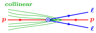
where λQCDΛQCD/Qsubscript𝜆QCDsubscriptΛQCD𝑄\lambda_{\mathrm{QCD}}\equiv\Lambda_{\mathrm{QCD}}/Q and λ𝜆\lambda are power-counting parameters. In this limit, illustrated in Fig. 1, L𝐿L has large Y𝑌Y while the emissions in X𝑋X become collimated in the opposite direction with typical momenta

pXμ(q+,Paq,pX)(q+,λ2q,λq+q).similar-tosuperscriptsubscript𝑝𝑋𝜇superscript𝑞superscriptsubscript𝑃𝑎superscript𝑞subscript𝑝perpendicular-to𝑋absentsimilar-tosuperscript𝑞superscript𝜆2superscript𝑞𝜆superscript𝑞superscript𝑞p_{X}^{\mu}\sim(q^{+},P_{a}^{-}-q^{-},p_{X\perp})\sim(q^{+},\lambda^{2}q^{-},\lambda\sqrt{q^{+}q^{-}})\,. (8)
Refer to caption
Figure 1: Illustration of Drell-Yan at large dilepton rapidity.

In this situation, the following factorization theorem holds to leading power in 1x1subscript𝑥1-x_{-},

dσdxdx+d𝜎dsubscript𝑥dsubscript𝑥\displaystyle\frac{\mathrm{d}\sigma}{\mathrm{d}x_{-}\mathrm{d}x_{+}} =Hij(q+q)dtfithr[x(1+tq+q)]absentsubscript𝐻𝑖𝑗superscript𝑞superscript𝑞differential-d𝑡superscriptsubscript𝑓𝑖thrdelimited-[]subscript𝑥1𝑡superscript𝑞superscript𝑞\displaystyle=H_{ij}(q^{+}q^{-})\int\!\mathrm{d}t\,f_{i}^{\mathrm{thr}}\Bigl{[}x_{-}\Bigl{(}1+\frac{t}{q^{+}q^{-}}\Bigr{)}\Bigr{]}
×Bj(t,x+).absentsubscript𝐵𝑗𝑡subscript𝑥\displaystyle\quad\times B_{j}(t,x_{+})\,. (9)

Here, Bj(t,x)subscript𝐵𝑗𝑡𝑥B_{j}(t,x) is the inclusive beam function that also appears in the factorization for N𝑁N-jettiness Stewart et al. (2010a, b). It depends on the transverse virtuality t𝑡t and momentum fraction x𝑥x of the colliding parton j𝑗j. Since tpX2λ2Q2ΛQCD2similar-to𝑡superscriptsubscript𝑝𝑋2similar-tosuperscript𝜆2superscript𝑄2much-greater-thansuperscriptsubscriptΛQCD2t\sim p_{X}^{2}\sim\lambda^{2}Q^{2}\gg\Lambda_{\mathrm{QCD}}^{2}, it can be calculated perturbatively in terms of standard PDFs as Stewart et al. (2010a, c)

Bj(t,x)=dzzjk(t,z)fk(xz).subscript𝐵𝑗𝑡𝑥d𝑧𝑧subscript𝑗𝑘𝑡𝑧subscript𝑓𝑘𝑥𝑧\displaystyle B_{j}(t,x)=\int\!\frac{\mathrm{d}z}{z}\,\mathcal{I}_{jk}(t,z)\,f_{k}\Bigl{(}\frac{x}{z}\Bigr{)}\,. (10)

The matching coefficients jksubscript𝑗𝑘\mathcal{I}_{jk} are known to 𝒪(αs2)𝒪superscriptsubscript𝛼𝑠2\mathcal{O}(\alpha_{s}^{2}) Stewart et al. (2010c); Berger et al. (2011); Gaunt et al. (2014a, b), with progress at 𝒪(αs3)𝒪superscriptsubscript𝛼𝑠3\mathcal{O}(\alpha_{s}^{3}) Melnikov et al. (2019a, b).

To derive Eq. (II), we use Soft-Collinear Effective Theory (SCET) Bauer et al. (2000, 2001); Bauer and Stewart (2001); Bauer et al. (2002a, b), which is the effective theory of QCD in the limit λ1much-less-than𝜆1\lambda\ll 1. The derivation proceeds in a standard fashion Stewart et al. (2010a), with more details given in *[SeeSupplementalMaterialattheendofthispreprint][]supplement. The key elements are the necessary degrees of freedom (modes) in the effective theory,

pn¯subscript𝑝¯𝑛\displaystyle p_{\bar{n}} Q(1,λ2,λ),Pn¯Q(1,λQCD2,λQCD),formulae-sequencesimilar-toabsent𝑄1superscript𝜆2𝜆similar-tosubscript𝑃¯𝑛𝑄1superscriptsubscript𝜆QCD2subscript𝜆QCD\displaystyle\sim Q\,\bigl{(}1,\lambda^{2},\lambda\bigr{)}\,,\quad P_{\bar{n}}\sim Q\,(1,\lambda_{\mathrm{QCD}}^{2},\lambda_{\mathrm{QCD}})\,, (11)
Pnsubscript𝑃𝑛\displaystyle P_{n} Q(λQCD2,1,λQCD),PsQ(λQCD2λ2,λ2,λQCD).formulae-sequencesimilar-toabsent𝑄superscriptsubscript𝜆QCD21subscript𝜆QCDsimilar-tosubscript𝑃𝑠𝑄superscriptsubscript𝜆QCD2superscript𝜆2superscript𝜆2subscript𝜆QCD\displaystyle\sim Q\,(\lambda_{\mathrm{QCD}}^{2},1,\lambda_{\mathrm{QCD}})\,,\quad P_{s}\sim Q\,\Bigl{(}\frac{\lambda_{\mathrm{QCD}}^{2}}{\lambda^{2}},\lambda^{2},\lambda_{\mathrm{QCD}}\Bigr{)}\,.

The pn¯subscript𝑝¯𝑛p_{\bar{n}} collinear modes describe the QCD final state at the scale λQ𝜆𝑄\lambda Q, which due to Eq. (8) is n¯¯𝑛{\bar{n}}-collinear. The Pn,n¯subscript𝑃𝑛¯𝑛P_{n,{\bar{n}}} collinear modes describe the PDFs at the scale λQCDQsubscript𝜆QCD𝑄\lambda_{\mathrm{QCD}}Q. The Pssubscript𝑃𝑠P_{s} modes describe the soft interactions between the pn¯subscript𝑝¯𝑛p_{\bar{n}} and Pnsubscript𝑃𝑛P_{n} modes. Possible ultrasoft/Glauber modes Pus,GQ(λQCD2,λQCD2,λQCD(2))similar-tosubscript𝑃𝑢𝑠𝐺𝑄superscriptsubscript𝜆QCD2superscriptsubscript𝜆QCD2superscriptsubscript𝜆QCD2P_{us,G}\sim Q(\lambda_{\mathrm{QCD}}^{2},\lambda_{\mathrm{QCD}}^{2},\lambda_{\mathrm{QCD}}^{(2)}) cancel as in Eq. (3) because the measurement is the same and its scale λQλQCDQmuch-greater-than𝜆𝑄subscript𝜆QCD𝑄\lambda Q\gg\lambda_{\mathrm{QCD}}Q.

The hard function Hijsubscript𝐻𝑖𝑗H_{ij} in Eq. (II) is the same as in Eq. (4). It arises from matching the electroweak current for L𝐿L onto the corresponding SCET current. There are no interactions between the modes in the leading-power SCET Lagrangian, so the complete matrix element factorizes into separate ones in each sector. The matrix element of the combined pn¯subscript𝑝¯𝑛p_{\bar{n}} and Pn¯subscript𝑃¯𝑛P_{\bar{n}} modes yields Bj(t,x)subscript𝐵𝑗𝑡𝑥B_{j}(t,x), and their separation leads to Eq. (10Stewart et al. (2010a, c). The combined matrix element of the Pnsubscript𝑃𝑛P_{n} and Pssubscript𝑃𝑠P_{s} modes yields fithrsuperscriptsubscript𝑓𝑖thrf_{i}^{\mathrm{thr}} Fleming and Labun (2015); Hoang et al. (2016). The convolution structure in Eq. (II) follows from momentum conservation sup .

Next, we consider also measuring qTsubscript𝑞𝑇\vec{\kern 0.0ptq}_{T}. From Eq. (8), it follows that generically qTpXλQsimilar-tosubscript𝑞𝑇subscript𝑝perpendicular-to𝑋absentsimilar-to𝜆𝑄q_{T}\sim p_{X\perp}\sim\lambda Q, so the qTsubscript𝑞𝑇q_{T} dependence is entirely described by the pn¯subscript𝑝¯𝑛p_{\bar{n}} modes, which yields the factorization theorem

dσdxdx+dqTd𝜎dsubscript𝑥dsubscript𝑥dsubscript𝑞𝑇\displaystyle\frac{\mathrm{d}\sigma}{\mathrm{d}x_{-}\mathrm{d}x_{+}\,\mathrm{d}\vec{\kern 0.0ptq}_{T}} =Hij(q+q)dtfithr[x(1+tq+q)]absentsubscript𝐻𝑖𝑗superscript𝑞superscript𝑞differential-d𝑡superscriptsubscript𝑓𝑖thrdelimited-[]subscript𝑥1𝑡superscript𝑞superscript𝑞\displaystyle=H_{ij}(q^{+}q^{-})\int\!\mathrm{d}t\,f_{i}^{\mathrm{thr}}\Bigl{[}x_{-}\Bigl{(}1+\frac{t}{q^{+}q^{-}}\Bigr{)}\Bigr{]}
×Bj(t,qT,x+).absentsubscript𝐵𝑗𝑡subscript𝑞𝑇subscript𝑥\displaystyle\quad\times B_{j}(t,\vec{\kern 0.0ptq}_{T},x_{+})\,. (12)

Here, Bj(t,kT,x)subscript𝐵𝑗𝑡subscript𝑘𝑇𝑥B_{j}(t,\vec{\kern 0.0ptk}_{T},x) is the double-differential beam function Jain et al. (2012); Gaunt and Stahlhofen (2014) that also occurs in the joint resummation of qTsubscript𝑞𝑇q_{T} and 00-jettiness Procura et al. (2015); Lustermans et al. (2019).

We can now change variables in Eq. (II) to xa,bsubscript𝑥𝑎𝑏x_{a,b}, using Eq. (6) and expanding in λ𝜆\lambda, which yields

dσdxadxbdqTd𝜎dsubscript𝑥𝑎dsubscript𝑥𝑏dsubscript𝑞𝑇\displaystyle\frac{\mathrm{d}\sigma}{\mathrm{d}x_{a}\mathrm{d}x_{b}\,\mathrm{d}\vec{\kern 0.0ptq}_{T}} =Hij(Q2)dtfithr[xa(1+qT22Q2+tQ2)]absentsubscript𝐻𝑖𝑗superscript𝑄2differential-d𝑡superscriptsubscript𝑓𝑖thrdelimited-[]subscript𝑥𝑎1superscriptsubscript𝑞𝑇22superscript𝑄2𝑡superscript𝑄2\displaystyle=H_{ij}(Q^{2})\int\!\mathrm{d}t\,f_{i}^{\mathrm{thr}}\Bigl{[}x_{a}\Bigl{(}1+\frac{q_{T}^{2}}{2Q^{2}}+\frac{t}{Q^{2}}\Bigr{)}\Bigr{]}
×Bj(t,qT,xb).absentsubscript𝐵𝑗𝑡subscript𝑞𝑇subscript𝑥𝑏\displaystyle\quad\times B_{j}(t,\vec{\kern 0.0ptq}_{T},x_{b})\,. (13)

Crucially, when expanding x=xa[1+qT2/(2Q2)+𝒪(λ4)]subscript𝑥subscript𝑥𝑎delimited-[]1superscriptsubscript𝑞𝑇22superscript𝑄2𝒪superscript𝜆4x_{-}=x_{a}[1+q_{T}^{2}/(2Q^{2})+\mathcal{O}(\lambda^{4})], we have to keep the qT2/(2Q2)λ2similar-tosuperscriptsubscript𝑞𝑇22superscript𝑄2superscript𝜆2q_{T}^{2}/(2Q^{2})\sim\lambda^{2} term in the PDF argument because it is of the same order as t/Q2λ2similar-to𝑡superscript𝑄2superscript𝜆2t/Q^{2}\sim\lambda^{2}. Integrating Eq. (II) over qTsubscript𝑞𝑇\vec{\kern 0.0ptq}_{T}, we obtain

dσdxadxb=Hij(Q2)dt~fithr[xa(1+t~Q2)]B~j(t~,xb).d𝜎dsubscript𝑥𝑎dsubscript𝑥𝑏subscript𝐻𝑖𝑗superscript𝑄2differential-d~𝑡superscriptsubscript𝑓𝑖thrdelimited-[]subscript𝑥𝑎1~𝑡superscript𝑄2subscript~𝐵𝑗~𝑡subscript𝑥𝑏\frac{\mathrm{d}\sigma}{\mathrm{d}x_{a}\mathrm{d}x_{b}}=H_{ij}(Q^{2})\!\int\!\mathrm{d}\tilde{t}\,f_{i}^{\mathrm{thr}}\Bigl{[}x_{a}\Bigl{(}1+\frac{\tilde{t}}{Q^{2}}\Bigr{)}\Bigr{]}\tilde{B}_{j}(\tilde{t},x_{b})\,. (14)

The factorization theorems in Eqs. (II) and (14) hold at leading power in the generalized threshold limit λ21xa1similar-tosuperscript𝜆21subscript𝑥𝑎much-less-than1\lambda^{2}\sim 1-x_{a}\ll 1 for generic xbsubscript𝑥𝑏x_{b}. They are our key new results.

In Eq. (14) we changed variables to t~=t+qT2/2~𝑡𝑡superscriptsubscript𝑞𝑇22\tilde{t}=t+q_{T}^{2}/2, and defined the new modified beam function

B~j(t~,x)=d2kTBj(t~kT22,kT,x).subscript~𝐵𝑗~𝑡𝑥superscriptd2subscript𝑘𝑇subscript𝐵𝑗~𝑡superscriptsubscript𝑘𝑇22subscript𝑘𝑇𝑥\displaystyle\tilde{B}_{j}(\tilde{t},x)=\int\mathrm{d}^{2}\vec{\kern 0.0ptk}_{T}\,B_{j}\Big{(}\tilde{t}-\frac{k_{T}^{2}}{2},\vec{\kern 0.0ptk}_{T},x\Big{)}\,. (15)

It has the same μ𝜇\mu evolution as Bj(t,x)subscript𝐵𝑗𝑡𝑥B_{j}(t,x) but different constant terms. It obeys a matching relation analogous to Eq. (10). Using the known results for Bj(t,kT,x)subscript𝐵𝑗𝑡subscript𝑘𝑇𝑥B_{j}(t,\vec{\kern 0.0ptk}_{T},x) Jain et al. (2012); Gaunt and Stahlhofen (2014), we have calculated its matching coefficients ~jk(t~,z)subscript~𝑗𝑘~𝑡𝑧\tilde{\mathcal{I}}_{jk}(\tilde{t},z) to 𝒪(αs2)𝒪superscriptsubscript𝛼𝑠2\mathcal{O}(\alpha_{s}^{2}) for j=q𝑗𝑞j=q and 𝒪(αs)𝒪subscript𝛼𝑠\mathcal{O}(\alpha_{s}) for j=g𝑗𝑔j=g sup .

The factorization structure in Eqs. (II) and (14) turns out to be analogous to deep-inelastic scattering (DIS) at large Bjorken x𝑥x Sterman (1987); Catani and Trentadue (1989); Manohar (2003); Becher et al. (2007); Fleming and Labun (2015); Chay and Kim (2013); Hoang et al. (2016), which factorizes as HijfithrJjtensor-productsubscript𝐻𝑖𝑗superscriptsubscript𝑓𝑖thrsubscript𝐽𝑗H_{ij}f_{i}^{\rm thr}\otimes J_{j}, with the jet function Jjsubscript𝐽𝑗J_{j} describing collimated final-state radiation. For Eqs. (II) and (14) to be consistent, the μ𝜇\mu dependence of the functions must cancel between them, and it does so in the same way as for DIS. The beam function is known to have the same μ𝜇\mu evolution as the jet function Stewart et al. (2010c). The existence of the above factorization theorems provides an independent confirmation of this. The key differences to DIS are the additional dependence on xbsubscript𝑥𝑏x_{b} and the nontrivial qTsubscript𝑞𝑇q_{T} dependence. The latter bears some resemblance to different 111-jettiness definitions in exclusive DIS Kang et al. (2013).

Since Eq. (14) is valid for xa1subscript𝑥𝑎1x_{a}\to 1 and arbitrary xbsubscript𝑥𝑏x_{b}, it must contain the soft threshold factorization in Eq. (4) for xb1subscript𝑥𝑏1x_{b}\to 1 as a special case. This implies sup

B~j(ωk,xb)=dk+ωS(k,k+)fjthr[xb(1+k+ω)]subscript~𝐵𝑗𝜔superscript𝑘subscript𝑥𝑏dsuperscript𝑘𝜔𝑆superscript𝑘superscript𝑘superscriptsubscript𝑓𝑗thrdelimited-[]subscript𝑥𝑏1superscript𝑘𝜔\tilde{B}_{j}(\omega k^{-}\!,x_{b})=\int\!\frac{\mathrm{d}k^{+}}{\omega}\,S(k^{-},k^{+})f_{j}^{\mathrm{thr}}\Bigl{[}x_{b}\Bigl{(}1+\frac{k^{+}}{\omega}\Bigr{)}\Bigr{]} (16)

to leading power in 1xb1subscript𝑥𝑏1-x_{b}, and identically for Bjsubscript𝐵𝑗B_{j}.

We can now combine Eq. (14) with the analogous result in the opposite limit xb1subscript𝑥𝑏1x_{b}\to 1 for generic xasubscript𝑥𝑎x_{a} by adding the two and subtracting their overlap, which is precisely given by the soft limit. This yields our main result, the generalized threshold factorization theorem

dσdxadxb=Hij[fithrB~j+B~ifjthrSfithrfjthr],d𝜎dsubscript𝑥𝑎dsubscript𝑥𝑏subscript𝐻𝑖𝑗delimited-[]tensor-productsuperscriptsubscript𝑓𝑖thrsubscript~𝐵𝑗tensor-productsubscript~𝐵𝑖superscriptsubscript𝑓𝑗thrtensor-product𝑆superscriptsubscript𝑓𝑖thrsuperscriptsubscript𝑓𝑗thr\displaystyle\frac{\mathrm{d}\sigma}{\mathrm{d}x_{a}\mathrm{d}x_{b}}=H_{ij}\Bigl{[}f_{i}^{\mathrm{thr}}\otimes\tilde{B}_{j}+\tilde{B}_{i}\otimes f_{j}^{\mathrm{thr}}-S\otimes f_{i}^{\mathrm{thr}}f_{j}^{\mathrm{thr}}\Bigr{]}\,, (17)

with the convolutions as in Eqs. (4) and (14). Analogous results hold for x±subscript𝑥plus-or-minusx_{\pm} and differential in qTsubscript𝑞𝑇\vec{\kern 0.0ptq}_{T}. Replacing fithr[x(1+1z)]superscriptsubscript𝑓𝑖thrdelimited-[]𝑥11𝑧f_{i}^{\mathrm{thr}}[x(1+1-z)] by fi(x/z)/zsubscript𝑓𝑖𝑥𝑧𝑧f_{i}(x/z)/z, which is justified at leading power in 1z1𝑧1-z, and comparing to Eq. (3), we obtain the corresponding partonic factorization theorem

σ^ij(za,zb)subscript^𝜎𝑖𝑗subscript𝑧𝑎subscript𝑧𝑏\displaystyle\hat{\sigma}_{ij}(z_{a},z_{b}) =Hk[δki^j(za,zb)+^ki(zb,za)δj\displaystyle=H_{k\ell}\bigl{[}\delta_{ki}\,\hat{\mathcal{I}}_{\ell j}(z_{a},z_{b})+\hat{\mathcal{I}}_{ki}(z_{b},z_{a})\,\delta_{\ell j}
δkiδjS^(za,zb)],\displaystyle\quad\quad\quad-\delta_{ki}\,\delta_{\ell j}\,\hat{S}(z_{a},z_{b})\bigr{]}\,, (18)

where we changed variables to za,bsubscript𝑧𝑎𝑏z_{a,b} and defined

^ij(za,zb)subscript^𝑖𝑗subscript𝑧𝑎subscript𝑧𝑏\displaystyle\hat{\mathcal{I}}_{ij}(z_{a},z_{b}) Q2~ij[Q2(1za),zb],absentsuperscript𝑄2subscript~𝑖𝑗superscript𝑄21subscript𝑧𝑎subscript𝑧𝑏\displaystyle\equiv Q^{2}\,\tilde{\mathcal{I}}_{ij}\bigl{[}Q^{2}(1-z_{a}),z_{b}\bigr{]}\,,
S^(za,zb)^𝑆subscript𝑧𝑎subscript𝑧𝑏\displaystyle\hat{S}(z_{a},z_{b}) Q2S[QeY(1za),QeY(1zb)].absentsuperscript𝑄2𝑆𝑄superscript𝑒𝑌1subscript𝑧𝑎𝑄superscript𝑒𝑌1subscript𝑧𝑏\displaystyle\equiv Q^{2}\,S\bigl{[}Qe^{Y}(1-z_{a}),Qe^{-Y}(1-z_{b})\bigr{]}\,. (19)
Refer to caption
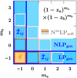
Figure 2: Terms in the partonic cross section σ^(za,zb)^𝜎subscript𝑧𝑎subscript𝑧𝑏\hat{\sigma}(z_{a},z_{b}) captured by the soft and generalized threshold expansions.

As illustrated in Fig. 2, ^ij(za,zb)subscript^𝑖𝑗subscript𝑧𝑎subscript𝑧𝑏\hat{\mathcal{I}}_{ij}(z_{a},z_{b}) captures all terms in σ^(za,zb)^𝜎subscript𝑧𝑎subscript𝑧𝑏\hat{\sigma}(z_{a},z_{b}) that are singular as za1subscript𝑧𝑎1z_{a}\to 1 with their exact dependence on zbsubscript𝑧𝑏z_{b}, and vice versa, with the overlap given by S^(za,zb)^𝑆subscript𝑧𝑎subscript𝑧𝑏\hat{S}(z_{a},z_{b}). This includes flavor-nondiagonal contributions, e.g., ij=qg𝑖𝑗𝑞𝑔ij=qg with k=qq¯𝑘𝑞¯𝑞k\ell=q{\bar{q}} or gg𝑔𝑔gg in Eq. (II).

III Validation

Refer to caption
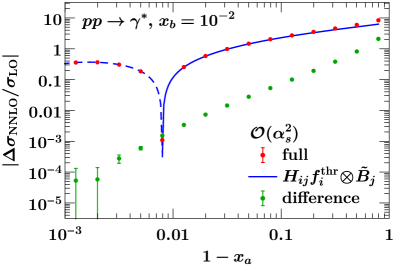
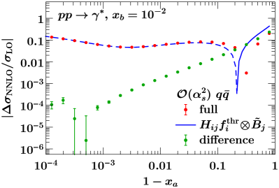
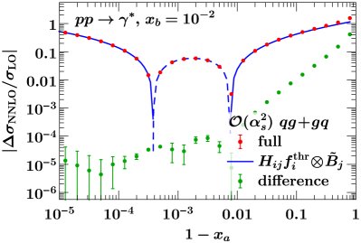
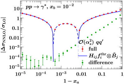
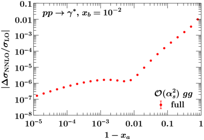
Figure 3: Validation of the 𝒪(αs2)𝒪superscriptsubscript𝛼𝑠2\mathcal{O}(\alpha_{s}^{2}) contribution to dσ/dxadxbd𝜎dsubscript𝑥𝑎dsubscript𝑥𝑏\mathrm{d}\sigma/\mathrm{d}x_{a}\mathrm{d}x_{b} predicted for xa1subscript𝑥𝑎1x_{a}\to 1 by Eq. (14) (blue) against the full result from Vrap (red). Their difference (green) vanishes like a power as 1xa01subscript𝑥𝑎01-x_{a}\to 0, as it must. The error bars indicate the integration uncertainties.

A nontrivial validation is to check Eq. (17) against the full fixed-order result. First, Eq. (16) implies

^ij(za,zb)subscript^𝑖𝑗subscript𝑧𝑎subscript𝑧𝑏\displaystyle\hat{\mathcal{I}}_{ij}(z_{a},z_{b}) =δijS^(za,zb)[1+𝒪(1zb)],absentsubscript𝛿𝑖𝑗^𝑆subscript𝑧𝑎subscript𝑧𝑏delimited-[]1𝒪1subscript𝑧𝑏\displaystyle=\delta_{ij}\,\hat{S}(z_{a},z_{b})\,\bigl{[}1+\mathcal{O}(1-z_{b})\bigr{]}\,, (20)

which we verified analytically to 𝒪(αs2)𝒪superscriptsubscript𝛼𝑠2\mathcal{O}(\alpha_{s}^{2}). It then suffices to check that Eq. (14) reproduces the fixed-order result for xa1subscript𝑥𝑎1x_{a}\to 1 (or za1subscript𝑧𝑎1z_{a}\to 1) for generic xbsubscript𝑥𝑏x_{b} (or zbsubscript𝑧𝑏z_{b}).

At NLO, we can check analytically for Drell-Yan and ggH𝑔𝑔𝐻gg\to H against the results of Refs. Anastasiou et al. (2003a, b), which are given as distributions in z=zazb𝑧subscript𝑧𝑎subscript𝑧𝑏z=z_{a}z_{b} and a variable y(za,zb)𝑦subscript𝑧𝑎subscript𝑧𝑏y(z_{a},z_{b}). Their translation to (za,zb)subscript𝑧𝑎subscript𝑧𝑏(z_{a},z_{b}) is nontrivial sup . We find complete agreement for all partonic channels. We also combined all singular terms from Eq. (II) with the regular terms from Refs. Anastasiou et al. (2003a, b) to construct the full σ^ij(za,zb)subscript^𝜎𝑖𝑗subscript𝑧𝑎subscript𝑧𝑏\hat{\sigma}_{ij}(z_{a},z_{b}) at NLO. The result is given in sup and agrees with Refs. Kubar et al. (1980); Mathews et al. (2005); Ravindran et al. (2007). 111 As discussed further in sup , several soft threshold factorizations differential in rapidity Bolzoni (2006); Mukherjee and Vogelsang (2006); Becher et al. (2008); Bonvini et al. (2011, 2015) differ from Eq. (4) and do not reproduce the correct soft limit already at NLO. .

At NNLO, we numerically validate our own implementation of Eq. (14) in SCETlib Ebert et al. (2018) against Vrap Anastasiou et al. (2004). We use flat PDFs, fithr(x)=fi(x)=θ(1x)superscriptsubscript𝑓𝑖thr𝑥subscript𝑓𝑖𝑥𝜃1𝑥f_{i}^{\mathrm{thr}}(x)=f_{i}(x)=\theta(1-x), which amounts to taking cumulant integrals of the partonic cross section and provides the strongest possible numerical check. In Fig. 3, we compare the 𝒪(αs2)𝒪superscriptsubscript𝛼𝑠2\mathcal{O}(\alpha_{s}^{2}) contribution for Drell-Yan as a function of 1xa1subscript𝑥𝑎1-x_{a} at fixed xb=102subscript𝑥𝑏superscript102x_{b}=10^{-2}. We find perfect agreement. The breakdown into partonic channels is given in sup . We also find similar agreement for other xbsubscript𝑥𝑏x_{b} and for ppZ/γ𝑝𝑝𝑍superscript𝛾pp\to Z/\gamma^{\ast} on the resonance.

IV Illustrative applications

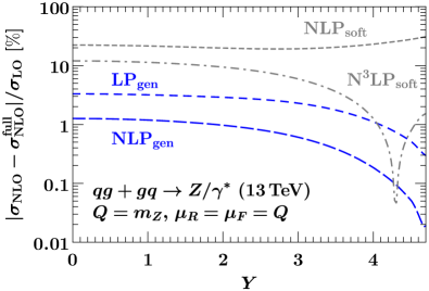
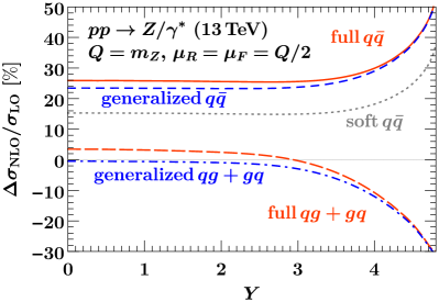
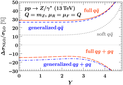
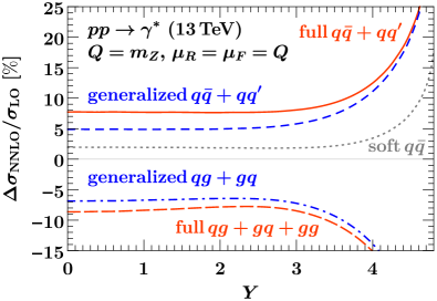
The immediate question that arises is how well the generalized threshold limit approximates the full fixed-order result for physical PDFs, particularly in comparison to the soft limit. We use the MMHT2014nnlo68cl Harland-Lang et al. (2015) PDFs, Vrap Anastasiou et al. (2004) to obtain the full NNLO result222 The public Vrap 0.9 assumes fq(x)=fq¯(x)subscript𝑓𝑞𝑥subscript𝑓¯𝑞𝑥f_{q}(x)=f_{\bar{q}}(x) for q=s,c,b𝑞𝑠𝑐𝑏q=s,c,b. We modified it to allow for different sea quark and antiquark PDFs. and SCETlib Ebert et al. (2018) to implement Eq. (II). In Fig. 4 we compare the 𝒪(αs)𝒪subscript𝛼𝑠\mathcal{O}(\alpha_{s}) and 𝒪(αs2)𝒪superscriptsubscript𝛼𝑠2\mathcal{O}(\alpha_{s}^{2}) contributions to the Drell-Yan rapidity spectrum at Q=mZ𝑄subscript𝑚𝑍Q=m_{Z}, separated into quark channels (qq¯+qq𝑞¯𝑞𝑞superscript𝑞q\bar{q}+qq^{\prime}) and channels involving a gluon (qg+gq+gg𝑞𝑔𝑔𝑞𝑔𝑔qg+gq+gg). Analogous results at μ=Q/2𝜇𝑄2\mu=Q/2 and for ggH𝑔𝑔𝐻gg\to H are provided in sup . The generalized threshold limit approximates the full result well for all channels and all Y𝑌Y. As expected, it works particularly well toward large Y𝑌Y. It works significantly better than the soft limit, which only provides a poor approximation for the qq¯𝑞¯𝑞q\bar{q} channel and none for the others. Currently, all ingredients are available to perform the resummation in the generalized threshold limit to N3LL, which we leave to future work. We expect it to be much more powerful for improving the precision of perturbative predictions than the soft threshold resummation.
Refer to caption
Refer to caption
Figure 4: The 𝒪(αs)𝒪subscript𝛼𝑠\mathcal{O}(\alpha_{s}) (top) and 𝒪(αs2)𝒪superscriptsubscript𝛼𝑠2\mathcal{O}(\alpha_{s}^{2}) (bottom) contributions to σdσ/dQdY𝜎d𝜎d𝑄d𝑌\sigma\equiv\mathrm{d}\sigma/\mathrm{d}Q\mathrm{d}Y normalized to the LO result. Shown are the full result (red), the generalized threshold approximation (blue), and the soft threshold approximation (gray).

Next, we may ask how well the power expansion around the generalized threshold limit works and how it relates to the soft expansion. Consider the double expansion in 1za1subscript𝑧𝑎1-z_{a} and 1zb1subscript𝑧𝑏1-z_{b}, illustrated in Fig. 2,

σ^ij(za,zb)=ma,mbσ^ij(ma,mb)(za,zb),subscript^𝜎𝑖𝑗subscript𝑧𝑎subscript𝑧𝑏subscriptsubscript𝑚𝑎subscript𝑚𝑏superscriptsubscript^𝜎𝑖𝑗subscript𝑚𝑎subscript𝑚𝑏subscript𝑧𝑎subscript𝑧𝑏\hat{\sigma}_{ij}(z_{a},z_{b})=\sum_{m_{a},m_{b}}\hat{\sigma}_{ij}^{(m_{a},m_{b})}(z_{a},z_{b})\,, (21)

where σ^ij(ma,mb)(za,zb)(1za)ma(1zb)mbsimilar-tosuperscriptsubscript^𝜎𝑖𝑗subscript𝑚𝑎subscript𝑚𝑏subscript𝑧𝑎subscript𝑧𝑏superscript1subscript𝑧𝑎subscript𝑚𝑎superscript1subscript𝑧𝑏subscript𝑚𝑏\hat{\sigma}_{ij}^{(m_{a},m_{b})}(z_{a},z_{b})\sim(1-z_{a})^{m_{a}}(1-z_{b})^{m_{b}}. Expanding around the soft z=zazb1𝑧subscript𝑧𝑎subscript𝑧𝑏1z=z_{a}z_{b}\to 1 limit corresponds to counting powers of (1z)ma+mb+1superscript1𝑧subscript𝑚𝑎subscript𝑚𝑏1(1-z)^{m_{a}+m_{b}+1}. The leading-power result in Eq. (5) gives the ma=mb=1subscript𝑚𝑎subscript𝑚𝑏1m_{a}=m_{b}=-1 term. At the m𝑚mth order, NmLPsoft, we keep all terms with ma+mb+2msubscript𝑚𝑎subscript𝑚𝑏2𝑚m_{a}+m_{b}+2\leq m. At leading power in the generalized expansion, Eq. (II) includes all terms with min{ma,mb}=1subscript𝑚𝑎subscript𝑚𝑏1\min\{m_{a},m_{b}\}=-1. Similarly, at the m𝑚mth order, NmLPgen, we keep all terms with min{ma,mb}=m1subscript𝑚𝑎subscript𝑚𝑏𝑚1\min\{m_{a},m_{b}\}=m-1, so the missing corrections at NmLPgen are 𝒪[(1za)m(1zb)m]𝒪delimited-[]superscript1subscript𝑧𝑎𝑚superscript1subscript𝑧𝑏𝑚\mathcal{O}[(1-z_{a})^{m}(1-z_{b})^{m}].

Refer to caption
Refer to caption
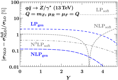
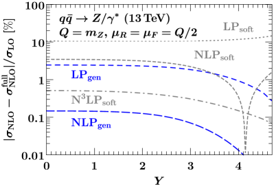
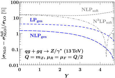
Figure 5: Convergence of the generalized (blue) and soft (gray) threshold expansions. Shown are the deviations from the full NLO result for the qq¯𝑞¯𝑞q\bar{q} channel (top) and the qg+gq𝑞𝑔𝑔𝑞qg+gq channel (bottom) normalized to the LO result.

In Fig. 5, we show the deviation from the exact result at various orders in both expansions for Drell-Yan at NLO, where we have full analytic control. Analogous results for ggH𝑔𝑔𝐻gg\to H are provided in sup . The generalized expansion performs significantly better than the soft one for both partonic channels. We expect this to hold in general, since expanding a two-dimensional function along a one-dimensional boundary is superior to expanding it in a single point on that boundary.

In fact, as seen in Fig. 2, each order in the generalized expansion fully contains two orders in the soft expansion, and in particular, the LPgen result Eq. (II) contains the entire NLPsoft contribution. This does not mean it can be used to perform the NLPsoft resummation because the μ𝜇\mu evolution of Bi(t,x)subscript𝐵𝑖𝑡𝑥B_{i}(t,x) does not predict its x𝑥x dependence. It does, however, show that Hijsubscript𝐻𝑖𝑗H_{ij} factorizes for all partonic channels and reduces the problem to deriving the NLPsoft factorization for Eq. (16).

At N3LO, Eq. (II) predicts a highly nontrivial set of terms for any color-singlet process, since all terms n(1za)similar-toabsentsubscript𝑛1subscript𝑧𝑎\sim\mathcal{L}_{n}(1-z_{a}) in ^ij(za,zb)subscript^𝑖𝑗subscript𝑧𝑎subscript𝑧𝑏\hat{\mathcal{I}}_{ij}(z_{a},z_{b}) are known from its μ𝜇\mu evolution, where n(y)[lnn(y)/y]+subscript𝑛𝑦subscriptdelimited-[]superscript𝑛𝑦𝑦\mathcal{L}_{n}(y)\equiv[\ln^{n}(y)/y]_{+}. To illustrate this, the coefficient of αs3/(4π)3superscriptsubscript𝛼𝑠3superscript4𝜋3\alpha_{s}^{3}/(4\pi)^{3} in σ^ij(μ=Q)subscript^𝜎𝑖𝑗𝜇𝑄\hat{\sigma}_{ij}(\mu=Q) with n3𝑛3n\geq 3 is

σ^ij(3)superscriptsubscript^𝜎𝑖𝑗3\displaystyle\hat{\sigma}_{ij}^{(3)} =5(1za)Hij(0)δ(1zb)(Γ0i)38absentsubscript51subscript𝑧𝑎subscriptsuperscript𝐻0𝑖𝑗𝛿1subscript𝑧𝑏superscriptsuperscriptsubscriptΓ0𝑖38\displaystyle=\mathcal{L}_{5}(1-z_{a})H^{(0)}_{ij}\delta(1-z_{b})\,\frac{(\Gamma_{0}^{i})^{3}}{8} (22)
+4(1za)Hik(0)[δkjδ(1zb)(2β03γB 0i2)\displaystyle\quad+\mathcal{L}_{4}(1-z_{a})H^{(0)}_{ik}\biggl{[}\delta_{kj}\delta(1-z_{b})\Bigl{(}-\frac{2\beta_{0}}{3}-\frac{\gamma_{B\,0}^{i}}{2}\Bigr{)}
+Pkj(0)(zb)]58(Γ0i)2+3(1za){Hij(1)δ(1zb)Γ0i2\displaystyle\quad+P^{(0)}_{kj}(z_{b})\biggr{]}\frac{5}{8}(\Gamma_{0}^{i})^{2}+\mathcal{L}_{3}(1-z_{a})\biggl{\{}H^{(1)}_{ij}\delta(1-z_{b})\frac{\Gamma_{0}^{i}}{2}
+Hik(0)[δkjδ(1zb)(Γ1iπ26(Γ0i)2+β023\displaystyle\quad+H^{(0)}_{ik}\biggl{[}\delta_{kj}\delta(1-z_{b})\Bigl{(}\Gamma_{1}^{i}-\frac{\pi^{2}}{6}(\Gamma_{0}^{i})^{2}+\frac{\beta_{0}^{2}}{3}
+(γB 0i)24+56β0γB 0i)P(0)kj(zb)(5β03+γB 0i)\displaystyle\quad+\frac{(\gamma_{B\,0}^{i})^{2}}{4}+\frac{5}{6}\beta_{0}\gamma_{B\,0}^{i}\Bigr{)}-P^{(0)}_{kj}(z_{b})\Bigl{(}\frac{5\beta_{0}}{3}+\gamma_{B\,0}^{i}\Bigr{)}
+(Pk(0)Pj(0))(zb)+I~kj(1)(zb)Γ0i2]}Γ0i+.\displaystyle\quad+\bigl{(}P^{(0)}_{k\ell}\otimes P^{(0)}_{\ell j}\bigr{)}(z_{b})+\tilde{I}^{(1)}_{kj}(z_{b})\,\frac{\Gamma_{0}^{i}}{2}\biggl{]}\biggr{\}}\Gamma_{0}^{i}+\dotsb\,.

The required ingredients are given in sup . The extension down to 0(1za)subscript01subscript𝑧𝑎\mathcal{L}_{0}(1-z_{a}) and to the full zasubscript𝑧𝑎z_{a} dependence for zb1subscript𝑧𝑏1z_{b}\to 1 is straightforward Billis et al. . The δ(1za)𝛿1subscript𝑧𝑎\delta(1-z_{a}) coefficient requires the still unknown 𝒪(αs3)𝒪superscriptsubscript𝛼𝑠3\mathcal{O}(\alpha_{s}^{3}) finite terms of the beam function. For Drell-Yan, Eq. (22) significantly extends the current knowledge at 𝒪(αs3)𝒪superscriptsubscript𝛼𝑠3\mathcal{O}(\alpha_{s}^{3}) Ahmed et al. (2014b), providing the full zbsubscript𝑧𝑏z_{b} dependence for all partonic channels. For ggH𝑔𝑔𝐻gg\to H, the extension to 0(1za)subscript01subscript𝑧𝑎\mathcal{L}_{0}(1-z_{a}) would also provide additional information beyond what is currently known Dulat et al. (2019).

V Summary

We introduced a generalized threshold factorization, which is much more powerful than the often used soft threshold, thus opening the door to numerous applications to improve theoretical predictions for collider processes. It describes all kinematic limits in (xa,xb)subscript𝑥𝑎subscript𝑥𝑏(x_{a},x_{b}) or (Q,Y)𝑄𝑌(Q,Y), including in particular |Y|Ymax𝑌subscript𝑌max\lvert Y\rvert\to Y_{\mathrm{max}} at generic Q𝑄Q, which is directly accessible at the LHC. It enables the corresponding threshold resummation where only one PDF is probed at large x𝑥x, which is not captured by the soft limit. At the partonic level, it captures all singularities of σ^ij(za,zb)subscript^𝜎𝑖𝑗subscript𝑧𝑎subscript𝑧𝑏\hat{\sigma}_{ij}(z_{a},z_{b}), including nondiagonal partonic channels. It can be used to predict a rich set of terms at higher fixed order or to resum them to all orders. It is the weakest known limit in which the process-dependent virtual corrections (Hijsubscript𝐻𝑖𝑗H_{ij}) factorize.

While we only considered color-singlet processes here, the same methods can be used to generalize the soft threshold factorization in other situations, such as for processes with heavy particles, jets, or identified hadrons in the final state.

Acknowledgements.
Acknowledgments

We thank M. Beneke, G. Billis, A. Broggio, G. Das, M. Diehl, L. Dixon, M. Ebert, S. Forte, A. Kulesza, S. Marzani, B. Mistlberger, F. Ringer, D. Scott, D. Soper, and W. Waalewijn for discussions. We thank M. Stahlhofen for providing the results of Ref. Gaunt and Stahlhofen (2014), and M. Prakash and V. Ravindran for help in comparing with Refs. Mathews et al. (2005); Ravindran et al. (2007). The authors thank each other’s institutions for hospitality. This work was supported in part by the ERC grant ERC-STG-2015-677323 and the D-ITP consortium, a program of the Netherlands Organization for Scientific Research (NWO) that is funded by the Dutch Ministry of Education, Culture and Science (OCW).

References

Supplemental material

V.1 Factorization theorem

Mode Lab frame Leptonic (Y^=0^𝑌0\hat{Y}=0) frame
(+,,)perpendicular-to(+,-,\perp) (+,,)perpendicular-to(+,-,\perp)
pn¯subscript𝑝¯𝑛p_{\bar{n}} (q+,λ2q,λqq+)superscript𝑞superscript𝜆2superscript𝑞𝜆superscript𝑞superscript𝑞(q^{+},\lambda^{2}q^{-},\lambda\sqrt{q^{-}q^{+}}) Q(1,λ2,λ)𝑄1superscript𝜆2𝜆Q\,(1,\lambda^{2},\lambda)
Pn¯subscript𝑃¯𝑛P_{\bar{n}} (q+,ΛQCD2q+,ΛQCD)superscript𝑞superscriptsubscriptΛQCD2superscript𝑞subscriptΛQCD\displaystyle\Bigl{(}q^{+},\frac{\Lambda_{\mathrm{QCD}}^{2}}{q^{+}},\Lambda_{\mathrm{QCD}}\Bigr{)} Q(1,λQCD2,λQCD)𝑄1superscriptsubscript𝜆QCD2subscript𝜆QCDQ\,(1,\lambda_{\mathrm{QCD}}^{2},\lambda_{\mathrm{QCD}})
Pnsubscript𝑃𝑛P_{n} (ΛQCD2q,q,ΛQCD)superscriptsubscriptΛQCD2superscript𝑞superscript𝑞subscriptΛQCD\displaystyle\Bigl{(}\frac{\Lambda_{\mathrm{QCD}}^{2}}{q^{-}},q^{-},\Lambda_{\mathrm{QCD}}\Bigr{)} Q(λQCD2,1,λQCD)𝑄superscriptsubscript𝜆QCD21subscript𝜆QCDQ\,(\lambda_{\mathrm{QCD}}^{2},1,\lambda_{\mathrm{QCD}})
Pssubscript𝑃𝑠P_{s} (1λ2ΛQCD2q,λ2q,ΛQCD)1superscript𝜆2superscriptsubscriptΛQCD2superscript𝑞superscript𝜆2superscript𝑞subscriptΛQCD\displaystyle\Bigl{(}\frac{1}{\lambda^{2}}\,\frac{\Lambda_{\mathrm{QCD}}^{2}}{q^{-}},\lambda^{2}q^{-},\Lambda_{\mathrm{QCD}}\Bigr{)} Q(λQCD2λ2,λ2,λQCD)𝑄superscriptsubscript𝜆QCD2superscript𝜆2superscript𝜆2subscript𝜆QCD\displaystyle Q\,\Bigl{(}\frac{\lambda_{\mathrm{QCD}}^{2}}{\lambda^{2}},\lambda^{2},\lambda_{\mathrm{QCD}}\Bigr{)}
Pussubscript𝑃𝑢𝑠P_{us} (ΛQCD2q,ΛQCD2q+,ΛQCD2q+q)superscriptsubscriptΛQCD2superscript𝑞superscriptsubscriptΛQCD2superscript𝑞superscriptsubscriptΛQCD2superscript𝑞superscript𝑞\displaystyle\Bigl{(}\frac{\Lambda_{\mathrm{QCD}}^{2}}{q^{-}},\frac{\Lambda_{\mathrm{QCD}}^{2}}{q^{+}},\frac{\Lambda_{\mathrm{QCD}}^{2}}{\sqrt{q^{+}q^{-}}}\Bigr{)} Q(λQCD2,λQCD2,λQCD2)𝑄superscriptsubscript𝜆QCD2superscriptsubscript𝜆QCD2superscriptsubscript𝜆QCD2Q\,(\lambda_{\mathrm{QCD}}^{2},\lambda_{\mathrm{QCD}}^{2},\lambda_{\mathrm{QCD}}^{2})
PGsubscript𝑃𝐺P_{G} (ΛQCD2q,ΛQCD2q+,ΛQCD)superscriptsubscriptΛQCD2superscript𝑞superscriptsubscriptΛQCD2superscript𝑞subscriptΛQCD\displaystyle\Bigl{(}\frac{\Lambda_{\mathrm{QCD}}^{2}}{q^{-}},\frac{\Lambda_{\mathrm{QCD}}^{2}}{q^{+}},\Lambda_{\mathrm{QCD}}\Bigr{)} Q(λQCD2,λQCD2,λQCD)𝑄superscriptsubscript𝜆QCD2superscriptsubscript𝜆QCD2subscript𝜆QCDQ\,(\lambda_{\mathrm{QCD}}^{2},\lambda_{\mathrm{QCD}}^{2},\lambda_{\mathrm{QCD}})
Table S1: Relevant EFT modes in the limit λQCDλ21x1similar-tosubscript𝜆QCDsuperscript𝜆2similar-to1superscript𝑥much-less-than1\lambda_{\mathrm{QCD}}\sim\lambda^{2}\sim 1-x^{-}\ll 1 in the lab (hadronic center-of-mass) frame and the leptonic frame where Y^=0^𝑌0\hat{Y}=0. In the right column we used that in the leptonic frame, q±q^±=q+qQsuperscript𝑞plus-or-minussuperscript^𝑞plus-or-minussuperscript𝑞superscript𝑞similar-to𝑄q^{\pm}\to\hat{q}^{\pm}=\sqrt{q^{+}q^{-}}\sim Q.

Here we give some more details on the derivation of the factorization theorem in Eq. (II), which underlies all other factorization theorems, and which we repeat here for easy reference,

dσdxdx+dqTd𝜎dsubscript𝑥dsubscript𝑥dsubscript𝑞𝑇\displaystyle\frac{\mathrm{d}\sigma}{\mathrm{d}x_{-}\mathrm{d}x_{+}\,\mathrm{d}\vec{\kern 0.0ptq}_{T}} =Hij(q+q)dtfithr[x(1+tq+q)]Bj(t,qT,x+).absentsubscript𝐻𝑖𝑗superscript𝑞superscript𝑞differential-d𝑡superscriptsubscript𝑓𝑖thrdelimited-[]subscript𝑥1𝑡superscript𝑞superscript𝑞subscript𝐵𝑗𝑡subscript𝑞𝑇subscript𝑥\displaystyle=H_{ij}(q^{+}q^{-})\int\!\mathrm{d}t\,f_{i}^{\mathrm{thr}}\Bigl{[}x_{-}\Bigl{(}1+\frac{t}{q^{+}q^{-}}\Bigr{)}\Bigr{]}B_{j}(t,\vec{\kern 0.0ptq}_{T},x_{+})\,. (S1)

As in the main text, we always implicitly sum over repeated flavor indices i,j,k𝑖𝑗𝑘i,j,k. Equation (S1) is valid up to power corrections in λ2superscript𝜆2\lambda^{2} in the generalized threshold limit

λ21x1for generic x+,λQCDΛQCD/Qλ2λ.formulae-sequencesimilar-tosuperscript𝜆21subscript𝑥much-less-than1for generic subscript𝑥subscript𝜆QCDsubscriptΛQCD𝑄similar-tosuperscript𝜆2much-less-than𝜆\lambda^{2}\sim 1-x_{-}\ll 1\qquad\text{for generic }x_{+}\,,\qquad\lambda_{\mathrm{QCD}}\equiv\Lambda_{\mathrm{QCD}}/Q\sim\lambda^{2}\ll\lambda\,. (S2)

We require λQCDλmuch-less-thansubscript𝜆QCD𝜆\lambda_{\mathrm{QCD}}\ll\lambda for reasons that will be apparent soon. Without loss of generality we can then consider λQCDλ2similar-tosubscript𝜆QCDsuperscript𝜆2\lambda_{\mathrm{QCD}}\sim\lambda^{2}. This relation is to be interpreted as follows: First, in our context, λQCDsubscript𝜆QCD\lambda_{\mathrm{QCD}} denotes the scale of the PDFs, which is generically allowed to be as large as λ2superscript𝜆2\lambda^{2} and does not necessarily have to be nonperturbative. If it happens to be a perturbative scale, then the physics below λQCDsubscript𝜆QCD\lambda_{\mathrm{QCD}} is simply described by the PDF evolution. Conversely, it also means that λ2superscript𝜆2\lambda^{2} is in principle allowed to be as small as λQCDsubscript𝜆QCD\lambda_{\mathrm{QCD}} including being nonperturbative, i.e., it is only relevant that λλQCDmuch-greater-than𝜆subscript𝜆QCD\lambda\gg\lambda_{\mathrm{QCD}} is perturbative.

The key step in deriving Eq. (S1) is to identify the relevant degrees of freedom (modes) in the effective field theory (EFT) that describe the physical situation. They are defined by the relative scaling of their light-cone momentum components and are summarized in Table S1. We note that rather than matching QCD directly onto these modes, one may also perform a multi-stage matching, as was done for endpoint DIS in Ref. Hoang et al. (2016), which yields the same end result.

The pn¯subscript𝑝¯𝑛p_{{\bar{n}}} modes describe the hadronic final state of the collision. Their scaling is determined by the fact that in the limit of Eq. (S2), there is only pn¯λ2Ecmλ2qsimilar-tosuperscriptsubscript𝑝¯𝑛superscript𝜆2subscript𝐸cmsimilar-tosuperscript𝜆2superscript𝑞p_{\bar{n}}^{-}\sim\lambda^{2}E_{\mathrm{cm}}\sim\lambda^{2}q^{-} minus momentum available. On the other hand, their plus momentum is unconstrained, which means it has generic scaling set by the hard interaction, pn¯+ξbEcmxbEcmq+similar-tosuperscriptsubscript𝑝¯𝑛subscript𝜉𝑏subscript𝐸cmsimilar-tosubscript𝑥𝑏subscript𝐸cmsimilar-tosuperscript𝑞p_{\bar{n}}^{+}\sim\xi_{b}E_{\mathrm{cm}}\sim x_{b}E_{\mathrm{cm}}\sim q^{+}. Since pn¯2λ2q+qλ2Q2ΛQCD2similar-tosuperscriptsubscript𝑝¯𝑛2superscript𝜆2superscript𝑞superscript𝑞similar-tosuperscript𝜆2superscript𝑄2much-greater-thansuperscriptsubscriptΛQCD2p_{\bar{n}}^{2}\sim\lambda^{2}q^{+}q^{-}\sim\lambda^{2}Q^{2}\gg\Lambda_{\mathrm{QCD}}^{2}, the pn¯subscript𝑝¯𝑛p_{\bar{n}} modes are perturbative. Therefore, they describe the perturbative QCD final state produced in the partonic collision in addition to L𝐿L (but excluding the beam remnant). The Pnsubscript𝑃𝑛P_{n} and Pn¯subscript𝑃¯𝑛P_{\bar{n}} modes describe the incoming protons, or more precisely, the partons in the proton with the typical momentum fractions required to produce the hard final state. This means their scaling is determined by Pnqsimilar-tosuperscriptsubscript𝑃𝑛superscript𝑞P_{n}^{-}\sim q^{-} and Pn¯+ξbEcmxbEcmq+similar-tosuperscriptsubscript𝑃¯𝑛subscript𝜉𝑏subscript𝐸cmsimilar-tosubscript𝑥𝑏subscript𝐸cmsimilar-tosuperscript𝑞P_{\bar{n}}^{+}\sim\xi_{b}E_{\mathrm{cm}}\sim x_{b}E_{\mathrm{cm}}\sim q^{+} and Pn2Pn¯2ΛQCD2similar-tosuperscriptsubscript𝑃𝑛2superscriptsubscript𝑃¯𝑛2similar-tosuperscriptsubscriptΛQCD2P_{n}^{2}\sim P_{\bar{n}}^{2}\sim\Lambda_{\mathrm{QCD}}^{2}.

The soft Pssubscript𝑃𝑠P_{s} modes describe the interactions between the pn¯subscript𝑝¯𝑛p_{\bar{n}} and Pnsubscript𝑃𝑛P_{n} modes. Their scaling is thus determined by Pspn¯λ2Qsimilar-tosuperscriptsubscript𝑃𝑠superscriptsubscript𝑝¯𝑛similar-tosuperscript𝜆2𝑄P_{s}^{-}\sim p_{\bar{n}}^{-}\sim\lambda^{2}Q and PsPnΛQCDsimilar-tosubscript𝑃perpendicular-to𝑠absentsubscript𝑃perpendicular-to𝑛absentsimilar-tosubscriptΛQCDP_{s\perp}\sim P_{n\perp}\sim\Lambda_{\mathrm{QCD}} or equivalently Ps2Pn2ΛQCD2similar-tosuperscriptsubscript𝑃𝑠2superscriptsubscript𝑃𝑛2similar-tosuperscriptsubscriptΛQCD2P_{s}^{2}\sim P_{n}^{2}\sim\Lambda_{\mathrm{QCD}}^{2}. Hence, they keep the pn¯subscript𝑝¯𝑛p_{\bar{n}} modes on shell and have a SCETI-like relation to them. Their interactions with the pn¯subscript𝑝¯𝑛p_{\bar{n}} modes in the leading-power SCET Lagrangian are decoupled and moved into soft Wilson lines in the SCET current via the BPS field redefinition. At the same time, the Pssubscript𝑃𝑠P_{s} modes have a SCETII-like relation to the Pnsubscript𝑃𝑛P_{n} modes, i.e., they have the same virtuality but are parametrically separated in rapidity. Hence, their interactions with the Pnsubscript𝑃𝑛P_{n} modes, which take the Pnsubscript𝑃𝑛P_{n} modes off shell, are described by soft Wilson lines in the SCET current that are directly produced during the matching onto SCET. The distinction of the Pssubscript𝑃𝑠P_{s} modes relies on λQCDλmuch-less-thansubscript𝜆QCD𝜆\lambda_{\mathrm{QCD}}\ll\lambda, while for λQCDλsimilar-tosubscript𝜆QCD𝜆\lambda_{\mathrm{QCD}}\sim\lambda, they would become degenerate with the pn¯subscript𝑝¯𝑛p_{\bar{n}} and Pn¯subscript𝑃¯𝑛P_{\bar{n}} modes.

The power counting and the relations between the modes are easiest in the leptonic frame, which is the frame where the color-singlet final state has total rapidity Y^=0^𝑌0\hat{Y}=0. Boosting from the lab frame to the leptonic frame by Y𝑌Y, we have q^±=q±e±Y=q+qQsuperscript^𝑞plus-or-minussuperscript𝑞plus-or-minussuperscript𝑒plus-or-minus𝑌superscript𝑞superscript𝑞similar-to𝑄\hat{q}^{\pm}=q^{\pm}e^{\pm Y}=\sqrt{q^{+}q^{-}}\sim Q. In the leptonic frame, the pn¯subscript𝑝¯𝑛p_{\bar{n}} modes are genuinely n¯¯𝑛{\bar{n}}-collinear with pn¯λ2pn¯+similar-tosuperscriptsubscript𝑝¯𝑛superscript𝜆2superscriptsubscript𝑝¯𝑛p_{\bar{n}}^{-}\sim\lambda^{2}p_{\bar{n}}^{+}, and the soft modes are homogeneous, Psλ2QλQCDQsimilar-tosubscript𝑃𝑠superscript𝜆2𝑄similar-tosubscript𝜆QCD𝑄P_{s}\sim\lambda^{2}Q\sim\lambda_{\mathrm{QCD}}Q. By contrast, in the lab frame we must separately keep track of q+superscript𝑞q^{+} and qsuperscript𝑞q^{-}, i.e., we cannot count them as q+qsimilar-tosuperscript𝑞superscript𝑞q^{+}\sim q^{-}, because we want to take the limit of large qsuperscript𝑞q^{-} for generic q+superscript𝑞q^{+}. As a result, the pn¯subscript𝑝¯𝑛p_{\bar{n}} modes do not necessarily appear to be n¯¯𝑛{\bar{n}}-collinear in the lab frame because q+λ2qsimilar-tosuperscript𝑞superscript𝜆2superscript𝑞q^{+}\sim\lambda^{2}q^{-} is allowed. However, the key requirement for their factorization is that they are collinear relative to the soft modes, which in the lab frame are boosted in the n𝑛n-collinear direction and become n𝑛n-collinear-soft (csoft) modes Bauer et al. (2012); Procura et al. (2015).

Finally, the ultrasoft (usoft) Pussubscript𝑃𝑢𝑠P_{us} and Glauber PGsubscript𝑃𝐺P_{G} modes describe the interactions between the Pnsubscript𝑃𝑛P_{n} and Pn¯subscript𝑃¯𝑛P_{\bar{n}} modes that are possible without pushing either of them off shell, which requires PusPn¯similar-tosuperscriptsubscript𝑃𝑢𝑠superscriptsubscript𝑃¯𝑛P_{us}^{-}\sim P_{\bar{n}}^{-} and Pus+Pn+similar-tosuperscriptsubscript𝑃𝑢𝑠superscriptsubscript𝑃𝑛P_{us}^{+}\sim P_{n}^{+}. The perpendicular-to\perp component of the usoft modes is fixed by requiring them to be on-shell modes, Pus2Pus+Pussimilar-tosuperscriptsubscript𝑃perpendicular-to𝑢𝑠absent2superscriptsubscript𝑃𝑢𝑠superscriptsubscript𝑃𝑢𝑠P_{us\perp}^{2}\sim P_{us}^{+}P_{us}^{-}. The corresponding Glauber modes are allowed to be off shell, so their perpendicular-to\perp component can be as large as PGPnPn¯ΛQCDsimilar-tosubscript𝑃perpendicular-to𝐺absentsubscript𝑃perpendicular-to𝑛absentsimilar-tosubscript𝑃perpendicular-to¯𝑛absentsimilar-tosubscriptΛQCDP_{G\perp}\sim P_{n\perp}\sim P_{{\bar{n}}\perp}\sim\Lambda_{\mathrm{QCD}}. The effects of the usoft and Glauber modes cancel, so we do not need to consider them further. This directly follows from the collinear factorization theorem Bodwin (1985); Collins et al. (1985, 1988) because in the limit we consider, the measurement is still fully inclusive over perpendicular momenta at the scale λQCDQsubscript𝜆QCD𝑄\lambda_{\mathrm{QCD}}Q. This is another reason why we require λQCDλmuch-less-thansubscript𝜆QCD𝜆\lambda_{\mathrm{QCD}}\ll\lambda. Note also that there is only a single collinear sector at the perturbative λQ𝜆𝑄\lambda Q scale, so there are no perturbative Glauber modes with scaling Q(λ2,λ2,λ)𝑄superscript𝜆2superscript𝜆2𝜆Q(\lambda^{2},\lambda^{2},\lambda) that could spoil factorization.

Since there are no interactions between the modes in the leading-power SCET Lagrangian, the cross section factorizes into separate forward matrix elements in each sector. The detailed derivation closely follows Ref. Stewart et al. (2010a), with the matrix element of the combined pn¯subscript𝑝¯𝑛p_{\bar{n}} and Pn¯subscript𝑃¯𝑛P_{\bar{n}} modes giving Bj(t,x)subscript𝐵𝑗𝑡𝑥B_{j}(t,x) and the combined matrix element of the Pnsubscript𝑃𝑛P_{n} and Pssubscript𝑃𝑠P_{s} modes giving fithrsuperscriptsubscript𝑓𝑖thrf_{i}^{\mathrm{thr}}. The factorization of the threshold PDF into separate collinear and csoft nonperturbative matrix elements is discussed in Refs. Fleming and Labun (2015); Hoang et al. (2016). It is not needed for our purposes. The arguments of the functions and their convolution structure in Eq. (S1) follow from overall momentum conservation among all sectors, which at leading power in λ𝜆\lambda must hold separately for the large (label) and small (residual) momenta carried by the matrix elements. Denoting them as ωn,n¯Qsimilar-tosubscript𝜔𝑛¯𝑛𝑄\omega_{n,{\bar{n}}}\sim Q, kn¯λQsimilar-tosubscript𝑘perpendicular-to¯𝑛absent𝜆𝑄k_{{\bar{n}}\perp}\sim\lambda Q, and ks,n¯λ2Qsimilar-tosubscript𝑘𝑠¯𝑛superscript𝜆2𝑄k_{s,{\bar{n}}}\sim\lambda^{2}Q, it takes the form

δ(ωn¯q+)δ(ωnq)δ(kn¯+qT)δ(kskn¯).𝛿subscript𝜔¯𝑛superscript𝑞𝛿subscript𝜔𝑛superscript𝑞𝛿subscript𝑘perpendicular-to¯𝑛absentsubscript𝑞𝑇𝛿superscriptsubscript𝑘𝑠superscriptsubscript𝑘¯𝑛\delta(\omega_{\bar{n}}-q^{+})\,\delta(\omega_{n}-q^{-})\,\delta(\vec{\kern 0.0ptk}_{{\bar{n}}\perp}+\vec{\kern 0.0ptq}_{T})\,\delta(k_{s}^{-}-k_{\bar{n}}^{-})\,. (S3)

The first three δ𝛿\delta functions set the x±subscript𝑥plus-or-minusx_{\pm} and qTsubscript𝑞𝑇\vec{\kern 0.0ptq}_{T} arguments of fithrsuperscriptsubscript𝑓𝑖thrf_{i}^{\rm thr} and Bjsubscript𝐵𝑗B_{j}. The analogous δ(ks+kn¯+)𝛿superscriptsubscript𝑘𝑠superscriptsubscript𝑘¯𝑛\delta(k_{s}^{+}-k_{\bar{n}}^{+}) disappeared by absorbing the kn¯+superscriptsubscript𝑘¯𝑛k_{\bar{n}}^{+} dependence into ωn¯subscript𝜔¯𝑛\omega_{\bar{n}} Stewart et al. (2010a). By combining the Pnsubscript𝑃𝑛P_{n} and Pssubscript𝑃𝑠P_{s} modes, the threshold PDF depends on (ωn+ks)/Pa=x(1+ks/q)subscript𝜔𝑛superscriptsubscript𝑘𝑠superscriptsubscript𝑃𝑎subscript𝑥1superscriptsubscript𝑘𝑠superscript𝑞(\omega_{n}+k_{s}^{-})/P_{a}^{-}=x_{-}(1+k_{s}^{-}/q^{-}). Here, we do have to keep track of the momentum of the Pssubscript𝑃𝑠P_{s} modes ksλ2Qsimilar-tosuperscriptsubscript𝑘𝑠superscript𝜆2𝑄k_{s}^{-}\sim\lambda^{2}Q, as it is much larger than the typical residual minus momentum knλQCD2Qsimilar-tosuperscriptsubscript𝑘𝑛superscriptsubscript𝜆QCD2𝑄k_{n}^{-}\sim\lambda_{\mathrm{QCD}}^{2}Q of the Pnsubscript𝑃𝑛P_{n} modes that is absorbed into ωnsubscript𝜔𝑛\omega_{n}. The δ(kskn¯)𝛿superscriptsubscript𝑘𝑠superscriptsubscript𝑘¯𝑛\delta(k_{s}^{-}-k_{\bar{n}}^{-}) then yields the convolution in t=q+kn¯𝑡superscript𝑞superscriptsubscript𝑘¯𝑛t=q^{+}k_{\bar{n}}^{-} in Eq. (S1). While Eq. (S1) is formally derived in the leptonic frame, it has exactly the same form in the lab frame. This is because the measured observables x±subscript𝑥plus-or-minusx_{\pm} and qTsubscript𝑞𝑇\vec{\kern 0.0ptq}_{T} are boost invariant along the beam axis, and reparametrization invariance (RPI) Manohar et al. (2002) forces all functions to only depend on boost-invariant quantities.

To see that the generalized threshold limit contains the soft threshold limit, note that the limits x1subscript𝑥1x_{-}\to 1 and x+1subscript𝑥1x_{+}\to 1 commute, so taking one limit after the other is equivalent to taking x,x+1subscript𝑥subscript𝑥1x_{-},x_{+}\to 1 simultaneously. To see this, consider the hierarchy λ21xλ+21x+1similar-tosuperscriptsubscript𝜆21subscript𝑥much-less-thansuperscriptsubscript𝜆2similar-to1subscript𝑥much-less-than1\lambda_{-}^{2}\sim 1-x_{-}\ll\lambda_{+}^{2}\sim 1-x_{+}\ll 1, which we can interpret as taking x+1subscript𝑥1x_{+}\to 1 after having already taken x1subscript𝑥1x_{-}\to 1. In this limit, the pn¯subscript𝑝¯𝑛p_{\bar{n}} modes factorize into perturbative n¯¯𝑛{\bar{n}}-csoft modes pn¯,csQ(λ+2,λ2,λ+λ)similar-tosubscript𝑝¯𝑛𝑐𝑠𝑄superscriptsubscript𝜆2superscriptsubscript𝜆2subscript𝜆subscript𝜆p_{{\bar{n}},cs}\sim Q(\lambda_{+}^{2},\lambda_{-}^{2},\lambda_{+}\lambda_{-}) and n¯¯𝑛{\bar{n}}-csoft modes Pn¯,csQ(λ+2,λQCD2/λ+2,λQCD)similar-tosubscript𝑃¯𝑛𝑐𝑠𝑄superscriptsubscript𝜆2superscriptsubscript𝜆QCD2superscriptsubscript𝜆2subscript𝜆QCDP_{{\bar{n}},cs}\sim Q(\lambda_{+}^{2},\lambda_{\mathrm{QCD}}^{2}/\lambda_{+}^{2},\lambda_{\mathrm{QCD}}). Including λ+subscript𝜆\lambda_{+}, the condition λQCDλmuch-less-thansubscript𝜆QCD𝜆\lambda_{\mathrm{QCD}}\ll\lambda becomes λQCDλλ+much-less-thansubscript𝜆QCDsubscript𝜆subscript𝜆\lambda_{\mathrm{QCD}}\ll\lambda_{-}\lambda_{+} and without loss of generality we can consider λQCDλ2λ+2similar-tosubscript𝜆QCDsuperscriptsubscript𝜆2superscriptsubscript𝜆2\lambda_{\mathrm{QCD}}\sim\lambda_{-}^{2}\lambda_{+}^{2}. This also implies that the Pssubscript𝑃𝑠P_{s} modes now get boosted in the n𝑛n direction and become n𝑛n-csoft modes, PsPn,cssubscript𝑃𝑠subscript𝑃𝑛𝑐𝑠P_{s}\equiv P_{n,cs}. The beam function matching onto PDFs now takes the form

Bj(ωn¯k,kT,x+)=dk+ωn¯𝒮(k,k+,kT)fjthr[x+(1+k+ωn¯)][1+𝒪(λ+)],subscript𝐵𝑗subscript𝜔¯𝑛superscript𝑘subscript𝑘𝑇subscript𝑥dsuperscript𝑘subscript𝜔¯𝑛𝒮superscript𝑘superscript𝑘subscript𝑘𝑇superscriptsubscript𝑓𝑗thrdelimited-[]subscript𝑥1superscript𝑘subscript𝜔¯𝑛delimited-[]1𝒪subscript𝜆B_{j}(\omega_{\bar{n}}k^{-},\vec{\kern 0.0ptk}_{T},x_{+})=\int\!\frac{\mathrm{d}k^{+}}{\omega_{\bar{n}}}\,\mathcal{S}(k^{-},k^{+},\vec{\kern 0.0ptk}_{T})\,f_{j}^{\mathrm{thr}}\Bigl{[}x_{+}\Bigl{(}1+\frac{k^{+}}{\omega_{\bar{n}}}\Bigr{)}\Bigr{]}\,\Bigl{[}1+\mathcal{O}(\lambda_{+})\Bigr{]}\,, (S4)

where the combined Pn¯,cssubscript𝑃¯𝑛𝑐𝑠P_{{\bar{n}},cs} and Pn¯subscript𝑃¯𝑛P_{\bar{n}} modes yield the threshold PDF, and 𝒮(k,k+,kT)𝒮superscript𝑘superscript𝑘subscript𝑘𝑇\mathcal{S}(k^{-},k^{+},\vec{\kern 0.0ptk}_{T}) is the matrix element of the pn¯,cssubscript𝑝¯𝑛𝑐𝑠p_{{\bar{n}},cs} modes. It has the same Wilson line structure as the soft function appearing in Eq. (4), and thus upon integration over kTsubscript𝑘𝑇\vec{\kern 0.0ptk}_{T} becomes equal to it to all orders by reparametrization invariance. We now have kT2/Q2λ2λ+2t/Q2λ2similar-tosuperscriptsubscript𝑘𝑇2superscript𝑄2superscriptsubscript𝜆2superscriptsubscript𝜆2much-less-than𝑡superscript𝑄2similar-tosuperscriptsubscript𝜆2k_{T}^{2}/Q^{2}\sim\lambda_{-}^{2}\lambda_{+}^{2}\ll t/Q^{2}\sim\lambda_{-}^{2}, so Bjsubscript𝐵𝑗B_{j} and B~jsubscript~𝐵𝑗\tilde{B}_{j} become the same and integrating Eq. (S4) over kTsubscript𝑘𝑇\vec{\kern 0.0ptk}_{T} yields Eq. (16) for either of them.

V.2 Plus distribution identities
Refer to caption
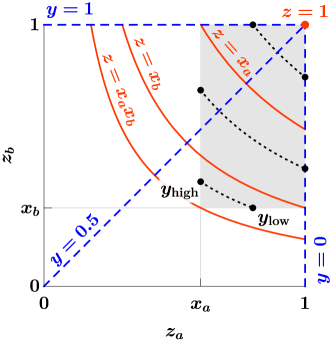
Figure S1: The (za,zb)subscript𝑧𝑎subscript𝑧𝑏(z_{a},z_{b}) plane as parametrized by (z,y)𝑧𝑦(z,y). The gray area shows the integration region xaza1subscript𝑥𝑎subscript𝑧𝑎1x_{a}\leq z_{a}\leq 1 and xbzb1subscript𝑥𝑏subscript𝑧𝑏1x_{b}\leq z_{b}\leq 1 (for the case of xa>xbsubscript𝑥𝑎subscript𝑥𝑏x_{a}>x_{b}) used to derive the distribution identities. The dotted black lines indicate integration paths over y𝑦y at representative fixed values of z𝑧z. The solid red lines indicate the edge cases in z𝑧z. The dashed blue lines are lines of constant y𝑦y.

In Refs. Anastasiou et al. (2003a, b, 2004), the partonic cross section for (Q,Y)𝑄𝑌(Q,Y) is given in terms of partonic variables (z,y)𝑧𝑦(z,y), defined as

z𝑧\displaystyle z =zazb,absentsubscript𝑧𝑎subscript𝑧𝑏\displaystyle=z_{a}z_{b}\,,\qquad y𝑦\displaystyle y =zb(1za2)(1zazb)(za+zb),absentsubscript𝑧𝑏1superscriptsubscript𝑧𝑎21subscript𝑧𝑎subscript𝑧𝑏subscript𝑧𝑎subscript𝑧𝑏\displaystyle=\frac{z_{b}(1-z_{a}^{2})}{(1-z_{a}z_{b})(z_{a}+z_{b})}\,,\qquad 1y1𝑦\displaystyle 1-y =za(1zb2)(1zazb)(za+zb)=y|ab,absentsubscript𝑧𝑎1superscriptsubscript𝑧𝑏21subscript𝑧𝑎subscript𝑧𝑏subscript𝑧𝑎subscript𝑧𝑏evaluated-at𝑦𝑎𝑏\displaystyle=\frac{z_{a}(1-z_{b}^{2})}{(1-z_{a}z_{b})(z_{a}+z_{b})}=y|_{a\leftrightarrow b}\,,
zasubscript𝑧𝑎\displaystyle z_{a} =z[1y(1z)]z+y(1z),absent𝑧delimited-[]1𝑦1𝑧𝑧𝑦1𝑧\displaystyle=\sqrt{\frac{z[1-y(1-z)]}{z+y(1-z)}}\,,\qquad zbsubscript𝑧𝑏\displaystyle z_{b} =za|y1y,absentevaluated-atsubscript𝑧𝑎𝑦1𝑦\displaystyle=z_{a}|_{y\leftrightarrow 1-y}\,,\qquad dzdydzadzbd𝑧d𝑦dsubscript𝑧𝑎dsubscript𝑧𝑏\displaystyle\frac{\mathrm{d}z\,\mathrm{d}y}{\mathrm{d}z_{a}\mathrm{d}z_{b}} =2[1y(1z)][1(1y)(1z)]1z2,absent2delimited-[]1𝑦1𝑧delimited-[]11𝑦1𝑧1superscript𝑧2\displaystyle=\frac{2[1-y(1-z)][1-(1-y)(1-z)]}{1-z^{2}}\,, (S5)

where za,bsubscript𝑧𝑎𝑏z_{a,b} are defined by Eq. (3), and the integration limits 0za,b10subscript𝑧𝑎𝑏10\leq z_{a,b}\leq 1 correspond to 0z10𝑧10\leq z\leq 1 and 0y10𝑦10\leq y\leq 1. In the following, we derive relations between plus distributions in (z,y)𝑧𝑦(z,y) and (za,zb)subscript𝑧𝑎subscript𝑧𝑏(z_{a},z_{b}).

In general, the plus distributions are uniquely defined by their functional form in the bulk, i.e. for za,b<1subscript𝑧𝑎𝑏1z_{a,b}<1 away from any singularity, and their integrals (against unit test functions) over arbitrary integration regions that include the singularities. First, the functional form in the bulk is easily obtained simply by plugging in Eq. (V.2). Next, the correct boundary terms at za=1subscript𝑧𝑎1z_{a}=1 as a function of zbsubscript𝑧𝑏z_{b}, at zb=1subscript𝑧𝑏1z_{b}=1 as a function of zasubscript𝑧𝑎z_{a}, and at za=zb=1subscript𝑧𝑎subscript𝑧𝑏1z_{a}=z_{b}=1 are determined by comparing integrals over the integration region xaza(z,y)1subscript𝑥𝑎subscript𝑧𝑎𝑧𝑦1x_{a}\leq z_{a}(z,y)\leq 1 and xbzb(z,y)1subscript𝑥𝑏subscript𝑧𝑏𝑧𝑦1x_{b}\leq z_{b}(z,y)\leq 1 for generic xasubscript𝑥𝑎x_{a} and xbsubscript𝑥𝑏x_{b}. This integration region is indicated by the gray box in the (za,zb)subscript𝑧𝑎subscript𝑧𝑏(z_{a},z_{b}) plane in Fig. S1. It is sufficiently general to fix all boundary terms and precisely corresponds to the relevant integration region for the physical cross section in (Q,Y)𝑄𝑌(Q,Y). In terms of (z,y)𝑧𝑦(z,y), the integration region is given by

θ[za(z,y)xa]θ[zb(z,y)xb]𝜃delimited-[]subscript𝑧𝑎𝑧𝑦subscript𝑥𝑎𝜃delimited-[]subscript𝑧𝑏𝑧𝑦subscript𝑥𝑏\displaystyle\theta\bigl{[}z_{a}(z,y)\geq x_{a}\bigr{]}\,\theta\bigl{[}z_{b}(z,y)\geq x_{b}\bigr{]} =θ[xaxbz<min{xa,xb}]θ[ylow(z)yyhigh(z)]+θ[max{xa,xb}z]absent𝜃delimited-[]subscript𝑥𝑎subscript𝑥𝑏𝑧subscript𝑥𝑎subscript𝑥𝑏𝜃delimited-[]subscript𝑦low𝑧𝑦subscript𝑦high𝑧𝜃delimited-[]subscript𝑥𝑎subscript𝑥𝑏𝑧\displaystyle=\theta\bigl{[}x_{a}x_{b}\leq z<\min\{x_{a},x_{b}\}\bigr{]}\,\theta\bigl{[}y_{\mathrm{low}}(z)\leq y\leq y_{\mathrm{high}}(z)\bigr{]}+\theta\bigl{[}\max\{x_{a},x_{b}\}\leq z\bigr{]}
+θ[xbz<xa]θ[yyhigh(z)]+θ(xaz<xb)θ[ylow(z)y],𝜃delimited-[]subscript𝑥𝑏𝑧subscript𝑥𝑎𝜃delimited-[]𝑦subscript𝑦high𝑧𝜃subscript𝑥𝑎𝑧subscript𝑥𝑏𝜃delimited-[]subscript𝑦low𝑧𝑦\displaystyle\quad+\theta\bigl{[}x_{b}\leq z<x_{a}\bigr{]}\,\theta\bigl{[}y\leq y_{\mathrm{high}}(z)\bigr{]}+\theta\bigl{(}x_{a}\leq z<x_{b})\,\theta\bigl{[}y_{\mathrm{low}}(z)\leq y\bigr{]}\,, (S6)

where the integration bounds in y𝑦y, also illustrated in Fig. S1, are given by

yhigh(z)=z(1xa2)(1z)(xa2+z),ylow(z)=xb2z2(1z)(z+xb2).formulae-sequencesubscript𝑦high𝑧𝑧1superscriptsubscript𝑥𝑎21𝑧superscriptsubscript𝑥𝑎2𝑧subscript𝑦low𝑧superscriptsubscript𝑥𝑏2superscript𝑧21𝑧𝑧superscriptsubscript𝑥𝑏2\displaystyle y_{\mathrm{high}}(z)=\frac{z(1-x_{a}^{2})}{(1-z)(x_{a}^{2}+z)}\,,\qquad y_{\mathrm{low}}(z)=\frac{x_{b}^{2}-z^{2}}{(1-z)(z+x_{b}^{2})}\,. (S7)

In Table S2, we collect the distribution identities at leading power in 1za1subscript𝑧𝑎1-z_{a} and arbitrary zbsubscript𝑧𝑏z_{b} that are required for validating Eq. (14) at NLO, where we denote the plus distributions as

n(x)=[θ(x)lnn(x)x]+=limϵ0ddx[θ(xϵ)lnn+1xn+1]withn(x>0)=lnn(x)x,1dxn(x)=0.formulae-sequencesubscript𝑛𝑥subscriptdelimited-[]𝜃𝑥superscript𝑛𝑥𝑥subscriptitalic-ϵ0dd𝑥delimited-[]𝜃𝑥italic-ϵsuperscript𝑛1𝑥𝑛1withsubscript𝑛𝑥0superscript𝑛𝑥𝑥superscript1differential-d𝑥subscript𝑛𝑥0\displaystyle\mathcal{L}_{n}(x)=\Bigl{[}\frac{\theta(x)\ln^{n}(x)}{x}\Bigr{]}_{+}=\lim_{\epsilon\to 0}\frac{\mathrm{d}}{\mathrm{d}x}\Bigl{[}\theta(x-\epsilon)\frac{\ln^{n+1}x}{n+1}\Bigr{]}\quad\text{with}\quad\mathcal{L}_{n}(x>0)=\frac{\ln^{n}(x)}{x}\,,\qquad\int^{1}\!\mathrm{d}x\,\mathcal{L}_{n}(x)=0\,. (S8)

The relations are derived by integrating each structure in the left column in terms of (z,y)𝑧𝑦(z,y) over the region in Eq. (V.2), expanding the result to leading power in 1xa1subscript𝑥𝑎1-x_{a}, and comparing to the corresponding (straightforward) integral over the same region in terms of za,bsubscript𝑧𝑎𝑏z_{a,b} of each structure in the right column.

dzdyLHSd𝑧d𝑦LHS\mathrm{d}z\,\mathrm{d}y\,\text{LHS} =dzadzbRHSabsentdsubscript𝑧𝑎dsubscript𝑧𝑏RHS=\mathrm{d}z_{a}\mathrm{d}z_{b}\,\text{RHS}
f(z)δ(y)𝑓𝑧𝛿𝑦f(z)\,\delta(y) f(zb)δ(1za)𝑓subscript𝑧𝑏𝛿1subscript𝑧𝑎f(z_{b})\,\delta(1-z_{a})
r(z)0(y)𝑟𝑧subscript0𝑦r(z)\,\mathcal{L}_{0}(y) r(zb)[0(1za)+δ(1za)ln2zb(1+zb)(1zb)]+𝒪(1)𝑟subscript𝑧𝑏delimited-[]subscript01subscript𝑧𝑎𝛿1subscript𝑧𝑎2subscript𝑧𝑏1subscript𝑧𝑏1subscript𝑧𝑏𝒪1\displaystyle r(z_{b})\Bigl{[}\mathcal{L}_{0}(1-z_{a})+\delta(1-z_{a})\,\ln\frac{2z_{b}}{(1+z_{b})(1-z_{b})}\Bigr{]}+\mathcal{O}(1)
f(z)δ(1y)𝑓𝑧𝛿1𝑦f(z)\,\delta(1-y) f(za)δ(1zb)𝑓subscript𝑧𝑎𝛿1subscript𝑧𝑏f(z_{a})\delta(1-z_{b})
r(z)0(1y)𝑟𝑧subscript01𝑦r(z)\,\mathcal{L}_{0}(1-y) 𝒪(1)𝒪1\mathcal{O}(1)
r(z)𝒪[y0(1y)0]𝑟𝑧𝒪delimited-[]superscript𝑦0superscript1𝑦0r(z)\,\mathcal{O}[y^{0}(1-y)^{0}] 𝒪(1)𝒪1\mathcal{O}(1)
0(1z)[0(y)+0(1y)]subscript01𝑧delimited-[]subscript0𝑦subscript01𝑦\mathcal{L}_{0}(1-z)\,\bigl{[}\mathcal{L}_{0}(y)+\mathcal{L}_{0}(1-y)\bigr{]} 1(1za)δ(1zb)+0(1za)0(1zb)δ(1za)1(1zb)subscript11subscript𝑧𝑎𝛿1subscript𝑧𝑏subscript01subscript𝑧𝑎subscript01subscript𝑧𝑏𝛿1subscript𝑧𝑎subscript11subscript𝑧𝑏\displaystyle-\mathcal{L}_{1}(1-z_{a})\,\delta(1-z_{b})+\mathcal{L}_{0}(1-z_{a})\,\mathcal{L}_{0}(1-z_{b})-\delta(1-z_{a})\,\mathcal{L}_{1}(1-z_{b})
+π26δ(1za)δ(1zb)+δ(1za)11zbln2zb1+zb+𝒪(1)superscript𝜋26𝛿1subscript𝑧𝑎𝛿1subscript𝑧𝑏𝛿1subscript𝑧𝑎11subscript𝑧𝑏2subscript𝑧𝑏1subscript𝑧𝑏𝒪1\displaystyle+\frac{\pi^{2}}{6}\delta(1-z_{a})\,\delta(1-z_{b})+\delta(1-z_{a})\,\frac{1}{1-z_{b}}\ln\frac{2z_{b}}{1+z_{b}}+\mathcal{O}(1)
Table S2: Translation identities of two-dimensional plus distributions between the (z,y)𝑧𝑦(z,y) and (za,zb)subscript𝑧𝑎subscript𝑧𝑏(z_{a},z_{b}) parametrizations. Here, f(x)𝑓𝑥f(x) is an arbitrary function of x𝑥x, potentially distribution-valued for x1𝑥1x\to 1, while r(x)=𝒪[(1x)0]𝑟𝑥𝒪delimited-[]superscript1𝑥0r(x)=\mathcal{O}[(1-x)^{0}] has at most an integrable singularity for x1𝑥1x\to 1. When indicated, the relations receive power corrections in 1za1subscript𝑧𝑎1-z_{a} starting at 𝒪(1)𝒪[(1za)0]𝒪1𝒪delimited-[]superscript1subscript𝑧𝑎0\mathcal{O}(1)\equiv\mathcal{O}[(1-z_{a})^{0}]. Overall factors of θ(1z)θ(y)θ(1y)=θ(1za)θ(1zb)𝜃1𝑧𝜃𝑦𝜃1𝑦𝜃1subscript𝑧𝑎𝜃1subscript𝑧𝑏\theta(1-z)\,\theta(y)\,\theta(1-y)=\theta(1-z_{a})\,\theta(1-z_{b}) are understood on both sides.

The last entry in Table S2 has the most intricate structure. Its exact integral without any expansion is given by

dzdyθ[za(z,y)xa]θ[zb(z,y)xb]0(1z)[0(y)+0(1y)]differential-d𝑧differential-d𝑦𝜃delimited-[]subscript𝑧𝑎𝑧𝑦subscript𝑥𝑎𝜃delimited-[]subscript𝑧𝑏𝑧𝑦subscript𝑥𝑏subscript01𝑧delimited-[]subscript0𝑦subscript01𝑦\displaystyle\int\!\mathrm{d}z\mathrm{d}y\,\theta\bigl{[}z_{a}(z,y)-x_{a}\bigr{]}\,\theta\bigl{[}z_{b}(z,y)-x_{b}\bigr{]}\,\mathcal{L}_{0}(1-z)\Bigl{[}\mathcal{L}_{0}(y)+\mathcal{L}_{0}(1-y)\Bigr{]}
=Fa(xa)+Fb(xb)Fa(xaxb)Fb(xaxb),absentsubscript𝐹𝑎subscript𝑥𝑎subscript𝐹𝑏subscript𝑥𝑏subscript𝐹𝑎subscript𝑥𝑎subscript𝑥𝑏subscript𝐹𝑏subscript𝑥𝑎subscript𝑥𝑏\displaystyle\qquad=F_{a}(x_{a})+F_{b}(x_{b})-F_{a}(x_{a}x_{b})-F_{b}(x_{a}x_{b})\,,
withFa,b(z)withsubscript𝐹𝑎𝑏𝑧\displaystyle\text{with}\qquad F_{a,b}(z) =ln(1z)ln(z+i0)Li2(1z1+xa,b)Li2(1z1xa,bi0)Li2(z),absent1𝑧𝑧i0subscriptLi21𝑧1subscript𝑥𝑎𝑏subscriptLi21𝑧1subscript𝑥𝑎𝑏i0subscriptLi2𝑧\displaystyle=-\ln(1-z)\ln(-z+\mathrm{i}0)-\text{Li}_{2}\Big{(}\frac{1-z}{1+x_{a,b}}\Big{)}-\text{Li}_{2}\Big{(}\frac{1-z}{1-x_{a,b}}-\mathrm{i}0\Big{)}-\text{Li}_{2}(z)\,, (S9)

where the imaginary parts from the branch cuts cancel between the different terms. Matching this with the exact distribution in the bulk, we obtain the distributional identity

dzdy0(1z)[0(y)+0(1y)]d𝑧d𝑦subscript01𝑧delimited-[]subscript0𝑦subscript01𝑦\displaystyle\mathrm{d}z\,\mathrm{d}y\,\mathcal{L}_{0}(1-z)\,\bigl{[}\mathcal{L}_{0}(y)+\mathcal{L}_{0}(1-y)\bigr{]}
=dzadzb[π26δ(1za)δ(1zb)1(1za)δ(1zb)+0(1za)0(1zb)δ(1za)1(1zb)\displaystyle\qquad=\mathrm{d}z_{a}\mathrm{d}z_{b}\biggl{[}\frac{\pi^{2}}{6}\,\delta(1-z_{a})\,\delta(1-z_{b})-\mathcal{L}_{1}(1-z_{a})\,\delta(1-z_{b})+\mathcal{L}_{0}(1-z_{a})\,\mathcal{L}_{0}(1-z_{b})-\delta(1-z_{a})\,\mathcal{L}_{1}(1-z_{b})
+δ(1za)11zbln2zb1+zb+δ(1zb)11zaln2za1+za+1(1+za)(1+zb)].\displaystyle\qquad\qquad\qquad\quad+\delta(1-z_{a})\,\frac{1}{1-z_{b}}\ln\frac{2z_{b}}{1+z_{b}}+\delta(1-z_{b})\,\frac{1}{1-z_{a}}\ln\frac{2z_{a}}{1+z_{a}}+\frac{1}{(1+z_{a})(1+z_{b})}\biggr{]}\,. (S10)

Expanding the right-hand side to leading power in 1za1subscript𝑧𝑎1-z_{a} yields the result given in the last line of Table S2. We note that Eq. (V.2) is the two-dimensional analog of a typical distribution identity like

[1+z21z]+=20(1z)+32δ(1z)(1+z).subscriptdelimited-[]1superscript𝑧21𝑧2subscript01𝑧32𝛿1𝑧1𝑧\displaystyle\Bigl{[}\frac{1+z^{2}}{1-z}\Bigr{]}_{+}=2\mathcal{L}_{0}(1-z)+\frac{3}{2}\delta(1-z)-(1+z)\,. (S11)

Namely, it expresses plus distributions of a function y(za,zb)𝑦subscript𝑧𝑎subscript𝑧𝑏y(z_{a},z_{b}) in terms of simpler plus distributions of 1za,b1subscript𝑧𝑎𝑏1-z_{a,b} plus regular terms. Moving the regular terms out of the plus distribution incurs additional boundary terms.

A key property of the left-hand side of Eq. (V.2) is that it vanishes when integrated over all of y𝑦y. It is instructive to see how this is reproduced by the right-hand side by projecting onto z𝑧z via dzadzbδ(zzazb)differential-dsubscript𝑧𝑎differential-dsubscript𝑧𝑏𝛿𝑧subscript𝑧𝑎subscript𝑧𝑏\int\!\mathrm{d}z_{a}\mathrm{d}z_{b}\,\delta(z-z_{a}z_{b}). The only nontrivial projection integral that is required is

dzadzbδ(zzazb)0(1za)0(1zb)=21(1z)π26δ(1z)lnz1z.differential-dsubscript𝑧𝑎differential-dsubscript𝑧𝑏𝛿𝑧subscript𝑧𝑎subscript𝑧𝑏subscript01subscript𝑧𝑎subscript01subscript𝑧𝑏2subscript11𝑧superscript𝜋26𝛿1𝑧𝑧1𝑧\int\!\mathrm{d}z_{a}\mathrm{d}z_{b}\,\delta(z-z_{a}z_{b})\,\mathcal{L}_{0}(1-z_{a})\mathcal{L}_{0}(1-z_{b})=2\mathcal{L}_{1}(1-z)-\frac{\pi^{2}}{6}\delta(1-z)-\frac{\ln z}{1-z}\,. (S12)

These terms precisely cancel the contributions from the other terms upon projecting onto z𝑧z.

V.3 Exact NLO partonic cross sections in terms of (𝒛𝒂,𝒛𝒃)subscript𝒛𝒂subscript𝒛𝒃(z_{a},z_{b})

Since Eq. (II) captures the full singularity structure as za1subscript𝑧𝑎1z_{a}\to 1 and/or zb1subscript𝑧𝑏1z_{b}\to 1, the power corrections to it are of relative 𝒪[(1za)(1zb)]𝒪delimited-[]1subscript𝑧𝑎1subscript𝑧𝑏\mathcal{O}[(1-z_{a})(1-z_{b})] and are fully integrable. Hence, we can construct the exact partonic cross section in terms of (za,zb)subscript𝑧𝑎subscript𝑧𝑏(z_{a},z_{b}) from the results in terms of (z,y)𝑧𝑦(z,y) from Refs. Anastasiou et al. (2003b, a) as

σ^ij(za,zb)subscript^𝜎𝑖𝑗subscript𝑧𝑎subscript𝑧𝑏\displaystyle\hat{\sigma}_{ij}(z_{a},z_{b}) =Hik^kj(za,zb)+Hkj^ki(zb,za)HijS^(za,zb)absentsubscript𝐻𝑖𝑘subscript^𝑘𝑗subscript𝑧𝑎subscript𝑧𝑏subscript𝐻𝑘𝑗subscript^𝑘𝑖subscript𝑧𝑏subscript𝑧𝑎subscript𝐻𝑖𝑗^𝑆subscript𝑧𝑎subscript𝑧𝑏\displaystyle=H_{ik}\hat{\mathcal{I}}_{kj}(z_{a},z_{b})+H_{kj}\hat{\mathcal{I}}_{ki}(z_{b},z_{a})-H_{ij}\hat{S}(z_{a},z_{b})
+[dzdydzadzbσ^ij[z(za,zb),y(za,zb)]Hik^kj(za,zb)Hkj^ki(zb,za)+HijS^(za,zb)]za,b<1.subscriptdelimited-[]d𝑧d𝑦dsubscript𝑧𝑎dsubscript𝑧𝑏subscript^𝜎𝑖𝑗𝑧subscript𝑧𝑎subscript𝑧𝑏𝑦subscript𝑧𝑎subscript𝑧𝑏subscript𝐻𝑖𝑘subscript^𝑘𝑗subscript𝑧𝑎subscript𝑧𝑏subscript𝐻𝑘𝑗subscript^𝑘𝑖subscript𝑧𝑏subscript𝑧𝑎subscript𝐻𝑖𝑗^𝑆subscript𝑧𝑎subscript𝑧𝑏subscript𝑧𝑎𝑏1\displaystyle\quad+\biggl{[}\frac{\mathrm{d}z\,\mathrm{d}y}{\mathrm{d}z_{a}\mathrm{d}z_{b}}\,\hat{\sigma}_{ij}\bigl{[}z(z_{a},z_{b}),y(z_{a},z_{b})\bigr{]}-H_{ik}\hat{\mathcal{I}}_{kj}(z_{a},z_{b})-H_{kj}\hat{\mathcal{I}}_{ki}(z_{b},z_{a})+H_{ij}\hat{S}(z_{a},z_{b})\biggr{]}_{z_{a,b}<1}\,. (S13)

Here, the term in square brackets is evaluated in the bulk, away from any singularities, so we can simply plug in Eq. (V.2). In the following, we collect the resulting expressions for the Drell-Yan and ggH𝑔𝑔𝐻gg\to H cross sections to NLO written explicitly in terms of (za,zb)subscript𝑧𝑎subscript𝑧𝑏(z_{a},z_{b}).

V.3.1 Results for Drell-Yan

The Born cross section for Drell-Yan production, qq¯Z/γ+𝑞¯𝑞𝑍superscript𝛾superscriptsuperscriptq\bar{q}\to Z/\gamma^{\ast}\to\ell^{+}\ell^{-}, is given by

σB,qDYsuperscriptsubscript𝜎𝐵𝑞DY\displaystyle\sigma_{B,q}^{\mathrm{DY}} =4παem23NcQ2[Qq2+(vq2+aq2)(v2+a2)2Qqvqv(1mZ2/Q2)(1mZ2/Q2)2+mZ2ΓZ2/Q4],absent4𝜋superscriptsubscript𝛼em23subscript𝑁𝑐superscript𝑄2delimited-[]superscriptsubscript𝑄𝑞2superscriptsubscript𝑣𝑞2superscriptsubscript𝑎𝑞2superscriptsubscript𝑣2superscriptsubscript𝑎22subscript𝑄𝑞subscript𝑣𝑞subscript𝑣1superscriptsubscript𝑚𝑍2superscript𝑄2superscript1superscriptsubscript𝑚𝑍2superscript𝑄22superscriptsubscript𝑚𝑍2superscriptsubscriptΓ𝑍2superscript𝑄4\displaystyle=\frac{4\pi\alpha_{\text{em}}^{2}}{3N_{c}Q^{2}}\biggl{[}Q_{q}^{2}+\frac{(v_{q}^{2}+a_{q}^{2})(v_{\ell}^{2}+a_{\ell}^{2})-2Q_{q}v_{q}v_{\ell}(1-m_{Z}^{2}/Q^{2})}{(1-m_{Z}^{2}/Q^{2})^{2}+m_{Z}^{2}\Gamma_{Z}^{2}/Q^{4}}\biggr{]}\,, (S14)

with Ncsubscript𝑁𝑐N_{c} the number of colors, Qqsubscript𝑄𝑞Q_{q} the quark charge in units of |e|𝑒\lvert e\rvert, v,qsubscript𝑣𝑞v_{\ell,q} and a,qsubscript𝑎𝑞a_{\ell,q} the standard electroweak vector and axial couplings of the leptons and quarks, and mZsubscript𝑚𝑍m_{Z} and ΓZsubscriptΓ𝑍\Gamma_{Z} the mass and width of the Z𝑍Z boson. To restrict to qq¯γ+𝑞¯𝑞superscript𝛾superscriptsuperscriptq\bar{q}\to\gamma^{\ast}\to\ell^{+}\ell^{-}, only the first term Qq2proportional-toabsentsuperscriptsubscript𝑄𝑞2\propto Q_{q}^{2} is kept. The complete LO cross section is given by

dσLODYdQdY=2QEcm2dσLODYdxadxb=2QEcm2qσB,qDY[fq(xa)fq¯(xb)+fq¯(xa)fq(xb)],dsubscriptsuperscript𝜎DYLOd𝑄d𝑌2𝑄superscriptsubscript𝐸cm2dsubscriptsuperscript𝜎DYLOdsubscript𝑥𝑎dsubscript𝑥𝑏2𝑄superscriptsubscript𝐸cm2subscript𝑞superscriptsubscript𝜎𝐵𝑞DYdelimited-[]subscript𝑓𝑞subscript𝑥𝑎subscript𝑓¯𝑞subscript𝑥𝑏subscript𝑓¯𝑞subscript𝑥𝑎subscript𝑓𝑞subscript𝑥𝑏\displaystyle\frac{\mathrm{d}\sigma^{\mathrm{DY}}_{\text{LO}}}{\mathrm{d}Q\,\mathrm{d}Y}=\frac{2Q}{E_{\mathrm{cm}}^{2}}\,\frac{\mathrm{d}\sigma^{\mathrm{DY}}_{\text{LO}}}{\mathrm{d}x_{a}\mathrm{d}x_{b}}=\frac{2Q}{E_{\mathrm{cm}}^{2}}\,\sum_{q}\sigma_{B,q}^{\mathrm{DY}}\,\bigl{[}f_{q}(x_{a})\,f_{\bar{q}}(x_{b})+f_{\bar{q}}(x_{a})\,f_{q}(x_{b})\bigr{]}\,, (S15)

where the sum runs over q={u,d,c,s,b}𝑞𝑢𝑑𝑐𝑠𝑏q=\{u,d,c,s,b\}. We expand the partonic cross section for Drell-Yan as

σ^ij(za,zb,Q,μ)=n=0[αs(μ)4π]nσij(n)(za,zb,Q,μ).subscript^𝜎𝑖𝑗subscript𝑧𝑎subscript𝑧𝑏𝑄𝜇superscriptsubscript𝑛0superscriptdelimited-[]subscript𝛼𝑠𝜇4𝜋𝑛superscriptsubscript𝜎𝑖𝑗𝑛subscript𝑧𝑎subscript𝑧𝑏𝑄𝜇\displaystyle\hat{\sigma}_{ij}(z_{a},z_{b},Q,\mu)=\sum_{n=0}^{\infty}\Bigl{[}\frac{\alpha_{s}(\mu)}{4\pi}\Bigr{]}^{n}\,\sigma_{ij}^{(n)}(z_{a},z_{b},Q,\mu)\,. (S16)

The LO result corresponding to Eq. (S15) is given by σ^qq¯(0)(za,zb,Q,μ)=σB,qDYδ(1za)δ(1zb)subscriptsuperscript^𝜎0𝑞¯𝑞subscript𝑧𝑎subscript𝑧𝑏𝑄𝜇superscriptsubscript𝜎𝐵𝑞DY𝛿1subscript𝑧𝑎𝛿1subscript𝑧𝑏\hat{\sigma}^{(0)}_{q{\bar{q}}}(z_{a},z_{b},Q,\mu)=\sigma_{B,q}^{\mathrm{DY}}\,\delta(1-z_{a})\,\delta(1-z_{b}). Writing z¯a1zasubscript¯𝑧𝑎1subscript𝑧𝑎{\bar{z}}_{a}\equiv 1-z_{a} and z¯b1zbsubscript¯𝑧𝑏1subscript𝑧𝑏{\bar{z}}_{b}\equiv 1-z_{b} for short, the NLO coefficient for the qq¯𝑞¯𝑞q{\bar{q}} channel is given by

1σB,qDYσ^qq¯(1)(za,zb,Q,μ)CF1superscriptsubscript𝜎𝐵𝑞DYsubscriptsuperscript^𝜎1𝑞¯𝑞subscript𝑧𝑎subscript𝑧𝑏𝑄𝜇subscript𝐶𝐹\displaystyle\frac{1}{\sigma_{B,q}^{\mathrm{DY}}}\frac{\hat{\sigma}^{(1)}_{q{\bar{q}}}(z_{a},z_{b},Q,\mu)}{C_{F}} =δ(z¯a)δ(z¯b)(2π216)+41(z¯a)δ(z¯b)+40(z¯a)0(z¯b)+4δ(z¯a)1(z¯b)absent𝛿subscript¯𝑧𝑎𝛿subscript¯𝑧𝑏2superscript𝜋2164subscript1subscript¯𝑧𝑎𝛿subscript¯𝑧𝑏4subscript0subscript¯𝑧𝑎subscript0subscript¯𝑧𝑏4𝛿subscript¯𝑧𝑎subscript1subscript¯𝑧𝑏\displaystyle=\delta({\bar{z}}_{a})\delta({\bar{z}}_{b})(2\pi^{2}-16)+4\mathcal{L}_{1}({\bar{z}}_{a})\delta({\bar{z}}_{b})+4\mathcal{L}_{0}({\bar{z}}_{a})\mathcal{L}_{0}({\bar{z}}_{b})+4\delta({\bar{z}}_{a})\mathcal{L}_{1}({\bar{z}}_{b})
+{2(1+zb)0(z¯a)+δ(z¯a)[2z¯b4(1+zb)lnz¯b2(1+zb2)lnzbz¯b\displaystyle\quad+\biggl{\{}-2(1+z_{b})\mathcal{L}_{0}({\bar{z}}_{a})+\delta({\bar{z}}_{a})\Bigl{[}2{\bar{z}}_{b}-4(1+z_{b})\ln{\bar{z}}_{b}-\frac{2(1+z_{b}^{2})\ln z_{b}}{{\bar{z}}_{b}}
+4z¯bln2zb1+zb+2(1+zb)ln1zb22zb]4lnμQδ(z¯a)[20(z¯b)+32δ(z¯b)(1+zb)]\displaystyle\qquad\quad+\frac{4}{{\bar{z}}_{b}}\ln\frac{2z_{b}}{1+z_{b}}+2(1+z_{b})\ln\frac{1-z_{b}^{2}}{2z_{b}}\Bigr{]}-4\ln\frac{\mu}{Q}\,\delta({\bar{z}}_{a})\Bigl{[}2\mathcal{L}_{0}({\bar{z}}_{b})+\frac{3}{2}\delta({\bar{z}}_{b})-(1+z_{b})\Bigr{]}
+2(za2+zb2)[(1+za)2+zazb(3+2za+zazb)](1+za)(1+zb)(za+zb)2+(zazb)},\displaystyle\qquad\quad+\frac{2(z_{a}^{2}+z_{b}^{2})[(1+z_{a})^{2}+z_{a}z_{b}(3+2z_{a}+z_{a}z_{b})]}{(1+z_{a})(1+z_{b})(z_{a}+z_{b})^{2}}+(z_{a}\leftrightarrow z_{b})\biggr{\}}\,, (S17)

where (zazb)subscript𝑧𝑎subscript𝑧𝑏(z_{a}\leftrightarrow z_{b}) indicates all previous expressions in the curly brackets repeated with zasubscript𝑧𝑎z_{a} and zbsubscript𝑧𝑏z_{b} interchanged. For the qg𝑞𝑔qg channel we have

1σB,qDYσ^qg(1)(za,zb,Q,μ)TF1superscriptsubscript𝜎𝐵𝑞DYsuperscriptsubscript^𝜎𝑞𝑔1subscript𝑧𝑎subscript𝑧𝑏𝑄𝜇subscript𝑇𝐹\displaystyle\frac{1}{\sigma_{B,q}^{\mathrm{DY}}}\frac{\hat{\sigma}_{qg}^{(1)}(z_{a},z_{b},Q,\mu)}{T_{F}} =2(zb2+z¯b2)0(z¯a)+δ(z¯a)[2(zb2+z¯b2)ln2z¯b1+zb+4zbz¯b]4lnμQδ(z¯a)(zb2+z¯b2)absent2superscriptsubscript𝑧𝑏2superscriptsubscript¯𝑧𝑏2subscript0subscript¯𝑧𝑎𝛿subscript¯𝑧𝑎delimited-[]2superscriptsubscript𝑧𝑏2superscriptsubscript¯𝑧𝑏22subscript¯𝑧𝑏1subscript𝑧𝑏4subscript𝑧𝑏subscript¯𝑧𝑏4𝜇𝑄𝛿subscript¯𝑧𝑎superscriptsubscript𝑧𝑏2superscriptsubscript¯𝑧𝑏2\displaystyle=2(z_{b}^{2}+{\bar{z}}_{b}^{2})\mathcal{L}_{0}({\bar{z}}_{a})+\delta({\bar{z}}_{a})\Bigl{[}2(z_{b}^{2}+{\bar{z}}_{b}^{2})\ln\frac{2{\bar{z}}_{b}}{1+z_{b}}+4z_{b}{\bar{z}}_{b}\Bigr{]}-4\ln\frac{\mu}{Q}\,\delta({\bar{z}}_{a})\bigl{(}z_{b}^{2}+{\bar{z}}_{b}^{2}\bigr{)} (S18)
+1(1+za)(za+zb)3[4za5zb34za4zb2(1+zb+2zb2)+2za3(1+4zb2+2zb34zb44zb5)\displaystyle\quad+\frac{1}{(1+z_{a})(z_{a}+z_{b})^{3}}\Bigl{[}-4z_{a}^{5}z_{b}^{3}-4z_{a}^{4}z_{b}^{2}(-1+z_{b}+2z_{b}^{2})+2z_{a}^{3}(1+4z_{b}^{2}+2z_{b}^{3}-4z_{b}^{4}-4z_{b}^{5})
+2za2zb(1+4zb+8zb28zb34zb4)+2zazb2(1+4zb2zb24zb3)2zb3(12zb+2zb2)].\displaystyle\qquad+2z_{a}^{2}z_{b}(1+4z_{b}+8z_{b}^{2}-8z_{b}^{3}-4z_{b}^{4})+2z_{a}z_{b}^{2}(1+4z_{b}-2z_{b}^{2}-4z_{b}^{3})-2z_{b}^{3}(1-2z_{b}+2z_{b}^{2})\Bigr{]}\,.

The gq𝑔𝑞gq channel is given by σgq(1)(Q,μ,za,zb)=σqg(1)(Q,μ,zb,za)superscriptsubscript𝜎𝑔𝑞1𝑄𝜇subscript𝑧𝑎subscript𝑧𝑏superscriptsubscript𝜎𝑞𝑔1𝑄𝜇subscript𝑧𝑏subscript𝑧𝑎\sigma_{gq}^{(1)}(Q,\mu,z_{a},z_{b})=\sigma_{qg}^{(1)}(Q,\mu,z_{b},z_{a}). The results for qq¯𝑞¯𝑞q\leftrightarrow{\bar{q}} are identical.

V.3.2 Results for gluon-fusion Higgs production

For gluon-fusion Higgs production, ggH𝑔𝑔𝐻gg\to H, we use the effective Lagrangian in the limit mH24mt2much-less-thansuperscriptsubscript𝑚𝐻24superscriptsubscript𝑚𝑡2m_{H}^{2}\ll 4m_{t}^{2},

eff(mH)=Ct12πvαsGμνaGa,μνH,Ct=1+αs4π(5CA3CF)+𝒪(αs2).formulae-sequencesubscripteffsubscript𝑚𝐻subscript𝐶𝑡12𝜋𝑣subscript𝛼𝑠superscriptsubscript𝐺𝜇𝜈𝑎superscript𝐺𝑎𝜇𝜈𝐻subscript𝐶𝑡1subscript𝛼𝑠4𝜋5subscript𝐶𝐴3subscript𝐶𝐹𝒪superscriptsubscript𝛼𝑠2\mathcal{L}_{\mathrm{eff}}(m_{H})=-\frac{C_{t}}{12\pi v}\,\alpha_{s}\,G_{\mu\nu}^{a}G^{a,\mu\nu}H\,,\qquad C_{t}=1+\frac{\alpha_{s}}{4\pi}(5C_{A}-3C_{F})+\mathcal{O}(\alpha_{s}^{2})\,. (S19)

As in Ref. Anastasiou et al. (2003a), the Wilson coefficient Ctsubscript𝐶𝑡C_{t} is always perturbatively expanded against other fixed-order contributions. The Born cross section and LO rapidity spectrum are given by

σBggH=172πv2(Nc21),dσLOggHdY=xaxbσBggHαs2fg(xa)fg(xb).formulae-sequencesuperscriptsubscript𝜎𝐵𝑔𝑔𝐻172𝜋superscript𝑣2superscriptsubscript𝑁𝑐21dsubscriptsuperscript𝜎𝑔𝑔𝐻LOd𝑌subscript𝑥𝑎subscript𝑥𝑏superscriptsubscript𝜎𝐵𝑔𝑔𝐻superscriptsubscript𝛼𝑠2subscript𝑓𝑔subscript𝑥𝑎subscript𝑓𝑔subscript𝑥𝑏\displaystyle\sigma_{B}^{ggH}=\frac{1}{72\pi v^{2}(N_{c}^{2}-1)}\,,\qquad\frac{\mathrm{d}\sigma^{ggH}_{\text{LO}}}{\mathrm{d}Y}=x_{a}x_{b}\,\sigma_{B}^{ggH}\,\alpha_{s}^{2}\,f_{g}(x_{a})\,f_{g}(x_{b})\,. (S20)

We write the partonic cross section as

σ^ij(za,zb,mt,mH,μ)σBggHαs2(μ)|Ct(mt,μ)|2n=0[αs(μ)4π]nη^ij(n)(za,zb,mH,μ).subscript^𝜎𝑖𝑗subscript𝑧𝑎subscript𝑧𝑏subscript𝑚𝑡subscript𝑚𝐻𝜇superscriptsubscript𝜎𝐵𝑔𝑔𝐻superscriptsubscript𝛼𝑠2𝜇superscriptsubscript𝐶𝑡subscript𝑚𝑡𝜇2superscriptsubscript𝑛0superscriptdelimited-[]subscript𝛼𝑠𝜇4𝜋𝑛superscriptsubscript^𝜂𝑖𝑗𝑛subscript𝑧𝑎subscript𝑧𝑏subscript𝑚𝐻𝜇\displaystyle\hat{\sigma}_{ij}(z_{a},z_{b},m_{t},m_{H},\mu)\equiv\sigma_{B}^{ggH}\,\alpha_{s}^{2}(\mu)\,|C_{t}(m_{t},\mu)|^{2}\,\sum_{n=0}^{\infty}\Bigl{[}\frac{\alpha_{s}(\mu)}{4\pi}\Bigr{]}^{n}\,\hat{\eta}_{ij}^{(n)}(z_{a},z_{b},m_{H},\mu)\,. (S21)

The NLO coefficient function for the gg𝑔𝑔gg channel is given by

η^gg(1)(za,zb,mH,μ)CAsuperscriptsubscript^𝜂𝑔𝑔1subscript𝑧𝑎subscript𝑧𝑏subscript𝑚𝐻𝜇subscript𝐶𝐴\displaystyle\frac{\hat{\eta}_{gg}^{(1)}(z_{a},z_{b},m_{H},\mu)}{C_{A}} =2π2δ(z¯a)δ(z¯b)+41(z¯a)δ(z¯b)+4δ(z¯a)1(z¯b)+40(z¯a)0(z¯b)absent2superscript𝜋2𝛿subscript¯𝑧𝑎𝛿subscript¯𝑧𝑏4subscript1subscript¯𝑧𝑎𝛿subscript¯𝑧𝑏4𝛿subscript¯𝑧𝑎subscript1subscript¯𝑧𝑏4subscript0subscript¯𝑧𝑎subscript0subscript¯𝑧𝑏\displaystyle=2\pi^{2}\delta({\bar{z}}_{a})\delta({\bar{z}}_{b})+4\mathcal{L}_{1}({\bar{z}}_{a})\delta({\bar{z}}_{b})+4\delta({\bar{z}}_{a})\mathcal{L}_{1}({\bar{z}}_{b})+4\mathcal{L}_{0}({\bar{z}}_{a})\mathcal{L}_{0}({\bar{z}}_{b}) (S22)
+{40(z¯a)[1zb2+zbzb2]+4δ(z¯a)1z¯b[ln(2z¯b)zb3lnz¯b+2ln1+zb2ln(1+zb)zb\displaystyle\quad+\biggl{\{}4\mathcal{L}_{0}({\bar{z}}_{a})\Bigl{[}\frac{1}{z_{b}}-2+z_{b}-z_{b}^{2}\Bigr{]}+4\delta({\bar{z}}_{a})\frac{1}{{\bar{z}}_{b}}\Bigl{[}\frac{\ln(2{\bar{z}}_{b})}{z_{b}}-3\ln{\bar{z}}_{b}+2\ln\frac{1+z_{b}}{2}-\frac{\ln(1+z_{b})}{z_{b}}
zb(32zb+zb2)ln1+zb2z¯b]4lnμmHδ(z¯a)[20(z¯b)(1zb+zb2)2zb]\displaystyle\qquad\quad-z_{b}(3-2z_{b}+z_{b}^{2})\ln\frac{1+z_{b}}{2{\bar{z}}_{b}}\Bigr{]}-4\ln\frac{\mu}{m_{H}}\delta({\bar{z}}_{a})\Bigl{[}2\mathcal{L}_{0}({\bar{z}}_{b})\frac{(1-z_{b}+z_{b}^{2})^{2}}{z_{b}}\Bigr{]}
+4zbza(1+za)(1+zb)(za+zb)4[2zb2+zb3+3za6zb4+2za5zb3(5+5zb+2zb2)\displaystyle\qquad\quad+\frac{4z_{b}}{z_{a}(1+z_{a})(1+z_{b})(z_{a}+z_{b})^{4}}\Bigl{[}2z_{b}^{2}+z_{b}^{3}+3z_{a}^{6}z_{b}^{4}+2z_{a}^{5}z_{b}^{3}(5+5z_{b}+2z_{b}^{2})
+za4zb2(16+17zb+12zb2+6zb3+2zb4)+za3zb(5+22zb+12zb2+8zb3+8zb4+2zb5)superscriptsubscript𝑧𝑎4superscriptsubscript𝑧𝑏21617subscript𝑧𝑏12superscriptsubscript𝑧𝑏26superscriptsubscript𝑧𝑏32superscriptsubscript𝑧𝑏4superscriptsubscript𝑧𝑎3subscript𝑧𝑏522subscript𝑧𝑏12superscriptsubscript𝑧𝑏28superscriptsubscript𝑧𝑏38superscriptsubscript𝑧𝑏42superscriptsubscript𝑧𝑏5\displaystyle\qquad\qquad+z_{a}^{4}z_{b}^{2}(16+17z_{b}+12z_{b}^{2}+6z_{b}^{3}+2z_{b}^{4})+z_{a}^{3}z_{b}(5+22z_{b}+12z_{b}^{2}+8z_{b}^{3}+8z_{b}^{4}+2z_{b}^{5})
+za2(3+2zb2+7zb3+2zb4+4zb5+2zb6)+zazb(4+zb+zb2+zb3+zb5)]+(zazb)}.\displaystyle\qquad\qquad+z_{a}^{2}(3+2z_{b}^{2}+7z_{b}^{3}+2z_{b}^{4}+4z_{b}^{5}+2z_{b}^{6})+z_{a}z_{b}(4+z_{b}+z_{b}^{2}+z_{b}^{3}+z_{b}^{5})\Bigr{]}+(z_{a}\leftrightarrow z_{b})\biggr{\}}\,.

For the gq𝑔𝑞gq and qg𝑞𝑔qg channels we find, with ηqg(1)(za,zb,mH,μ)=ηgq(1)(zb,za,mH,μ)superscriptsubscript𝜂𝑞𝑔1subscript𝑧𝑎subscript𝑧𝑏subscript𝑚𝐻𝜇superscriptsubscript𝜂𝑔𝑞1subscript𝑧𝑏subscript𝑧𝑎subscript𝑚𝐻𝜇\eta_{qg}^{(1)}(z_{a},z_{b},m_{H},\mu)=\eta_{gq}^{(1)}(z_{b},z_{a},m_{H},\mu),

η^gq(1)(za,zb,mH,μ)CFsuperscriptsubscript^𝜂𝑔𝑞1subscript𝑧𝑎subscript𝑧𝑏subscript𝑚𝐻𝜇subscript𝐶𝐹\displaystyle\frac{\hat{\eta}_{gq}^{(1)}(z_{a},z_{b},m_{H},\mu)}{C_{F}} =20(z¯a)22zb+zb2zb+2δ(z¯a)[zb+22zb+zb2zb(ln2z¯b1+zb2lnμmH)]absent2subscript0subscript¯𝑧𝑎22subscript𝑧𝑏superscriptsubscript𝑧𝑏2subscript𝑧𝑏2𝛿subscript¯𝑧𝑎delimited-[]subscript𝑧𝑏22subscript𝑧𝑏superscriptsubscript𝑧𝑏2subscript𝑧𝑏2subscript¯𝑧𝑏1subscript𝑧𝑏2𝜇subscript𝑚𝐻\displaystyle=2\mathcal{L}_{0}({\bar{z}}_{a})\,\frac{2-2z_{b}+z_{b}^{2}}{z_{b}}+2\delta({\bar{z}}_{a})\Bigl{[}z_{b}+\frac{2-2z_{b}+z_{b}^{2}}{z_{b}}\Bigl{(}\ln\frac{2{\bar{z}}_{b}}{1+z_{b}}-2\ln\frac{\mu}{m_{H}}\Bigr{)}\Bigr{]}
+2(1+za)zb(za+zb)3[za3(22zb+zb2)+za2(42zb4zb2+7zb32zb5)\displaystyle\quad+\frac{2}{(1+z_{a})z_{b}(z_{a}+z_{b})^{3}}\Bigl{[}z_{a}^{3}(2-2z_{b}+z_{b}^{2})+z_{a}^{2}(4-2z_{b}-4z_{b}^{2}+7z_{b}^{3}-2z_{b}^{5})
+zazb(44zb+4zb2+zb32zb4)zb2(2+2zb2zb2+zb3)].\displaystyle\qquad+z_{a}z_{b}(4-4z_{b}+4z_{b}^{2}+z_{b}^{3}-2z_{b}^{4})-z_{b}^{2}(-2+2z_{b}-2z_{b}^{2}+z_{b}^{3})\Bigr{]}\,. (S23)

The qq¯𝑞¯𝑞q\bar{q} channel is fully regular and given by

η^qq¯(1)(za,zb,mH,μ)CF=Nc21Nc4(1+zazb)(za4zb2+za2zb44za2zb2+za2+zb2)(za+zb)4.superscriptsubscript^𝜂𝑞¯𝑞1subscript𝑧𝑎subscript𝑧𝑏subscript𝑚𝐻𝜇subscript𝐶𝐹superscriptsubscript𝑁𝑐21subscript𝑁𝑐41subscript𝑧𝑎subscript𝑧𝑏superscriptsubscript𝑧𝑎4superscriptsubscript𝑧𝑏2superscriptsubscript𝑧𝑎2superscriptsubscript𝑧𝑏44superscriptsubscript𝑧𝑎2superscriptsubscript𝑧𝑏2superscriptsubscript𝑧𝑎2superscriptsubscript𝑧𝑏2superscriptsubscript𝑧𝑎subscript𝑧𝑏4\displaystyle\frac{\hat{\eta}_{q\bar{q}}^{(1)}(z_{a},z_{b},m_{H},\mu)}{C_{F}}=\frac{N_{c}^{2}-1}{N_{c}}\,\frac{4(1+z_{a}z_{b})(z_{a}^{4}z_{b}^{2}+z_{a}^{2}z_{b}^{4}-4z_{a}^{2}z_{b}^{2}+z_{a}^{2}+z_{b}^{2})}{(z_{a}+z_{b})^{4}}\,. (S24)

The Ncsubscript𝑁𝑐N_{c}-dependent prefactor accounts for the different color average compared to the Born cross section.

The above expressions are in full agreement with Refs. Mathews et al. (2005); Ravindran et al. (2007), which in turn agree with the earliest result for the NLO Drell-Yan rapidity spectrum in Ref. Kubar et al. (1980). In Refs. Mathews et al. (2005); Ravindran et al. (2007), the cross section was also parametrized in terms of xa,bsubscript𝑥𝑎𝑏x_{a,b} and za,bsubscript𝑧𝑎𝑏z_{a,b}, but all subtractions were written out in full at the level of the hadronic cross section.

In Ref. Anastasiou et al. (2003b), only the sum of the gq𝑔𝑞gq and qg𝑞𝑔qg coefficient functions for Higgs productions was given. The separation of the singular terms into the two channels is unique because only the gq𝑔𝑞gq (qg𝑞𝑔qg) channel can be singular as y0𝑦0y\to 0 (y1𝑦1y\to 1). We determined the separation of the regular terms by comparing to Ref. Ravindran et al. (2007). To the best of our knowledge, this is the first time that the explicit analytic agreement between the independent NLO calculations in terms of (za,zb)subscript𝑧𝑎subscript𝑧𝑏(z_{a},z_{b}) and (z,y)𝑧𝑦(z,y) has been established.

Finally, we have also compared our numerical implementation of Eq. (S16)-(S24) with the rapidity spectra obtained from Vrap 0.9 Anastasiou et al. (2004) for Drell-Yan and from SusHi 1.7.0 Harlander et al. (2013, 2017) for Higgs production, finding excellent agreement. Since Vrap 0.9 implements the (z,y)𝑧𝑦(z,y) parametrization, this effectively confirms the distributional identities in Table S2 numerically with physical PDFs as test functions.

V.4 Comment on rapidity-dependent soft threshold results in the literature

As we have discussed, the soft threshold limit is fully contained in the generalized threshold limit. Our results thus provide an independent confirmation that Eq. (4) is the correct soft threshold factorization for the cross section differential in both Q𝑄Q and Y𝑌Y, or equivalently Eq. (5) for the two-dimensional partonic cross section in (za,zb)subscript𝑧𝑎subscript𝑧𝑏(z_{a},z_{b}).

Several results in the literature Bolzoni (2006); Mukherjee and Vogelsang (2006); Becher et al. (2008); Bonvini et al. (2011, 2015) considering the soft threshold factorization differential in rapidity differ from Eq. (4). The difference is manifest already at fixed NLO in the term 0(1z)[0(y)+0(1y)]subscript01𝑧delimited-[]subscript0𝑦subscript01𝑦\mathcal{L}_{0}(1-z)[\mathcal{L}_{0}(y)+\mathcal{L}_{0}(1-y)], which appears in the flavor-diagonal partonic cross sections. The distributional identity in Eq. (V.2) unambiguously shows that this term has a double singularity in the limit za1subscript𝑧𝑎1z_{a}\to 1 and zb1subscript𝑧𝑏1z_{b}\to 1, which means it contributes a priori at leading power in the soft limit z=zazb1𝑧subscript𝑧𝑎subscript𝑧𝑏1z=z_{a}z_{b}\to 1, i.e., it contributes to the ma=mb=1subscript𝑚𝑎subscript𝑚𝑏1m_{a}=m_{b}=-1 term in Eq. (21). This can already be seen just by considering the distribution in the bulk since

dzdy11z(1y+11y)=dzadzb1(1za)(1zb)[1+𝒪(1za,1zb)].d𝑧d𝑦11𝑧1𝑦11𝑦dsubscript𝑧𝑎dsubscript𝑧𝑏11subscript𝑧𝑎1subscript𝑧𝑏delimited-[]1𝒪1subscript𝑧𝑎1subscript𝑧𝑏\mathrm{d}z\,\mathrm{d}y\,\frac{1}{1-z}\Bigl{(}\frac{1}{y}+\frac{1}{1-y}\Bigr{)}=\mathrm{d}z_{a}\mathrm{d}z_{b}\,\frac{1}{(1-z_{a})(1-z_{b})}\bigl{[}1+\mathcal{O}(1-z_{a},1-z_{b})\bigr{]}\,. (S25)

Moreover, Eq. (V.2) shows that it contributes at leading-logarithmic order. The soft function in Eqs. (4) and (5) precisely contains the leading-power contribution of this term, which is given by the first four terms on the right-hand side of Eq. (V.2).

By contrast, this term and analogous ones at higher order are missing in the leading-power resummed results in Refs. Bolzoni (2006); Mukherjee and Vogelsang (2006); Becher et al. (2008); Bonvini et al. (2011, 2015). There, it is effectively argued that the contribution of such terms to the rapidity spectrum is power-suppressed in 1z1𝑧1-z, leading to the incorrect conclusion that the rapidity dependence in the soft threshold limit can be included simply by taking σ^ij(za,zb)subscript^𝜎𝑖𝑗subscript𝑧𝑎subscript𝑧𝑏\hat{\sigma}_{ij}(z_{a},z_{b}) to be σ^ij(z)[δ(y)+δ(1y)]/2subscript^𝜎𝑖𝑗𝑧delimited-[]𝛿𝑦𝛿1𝑦2\hat{\sigma}_{ij}(z)\,[\delta(y)+\delta(1-y)]/2 or, depending on the reference, σ^ij(z)δ(y1/2)subscript^𝜎𝑖𝑗𝑧𝛿𝑦12\hat{\sigma}_{ij}(z)\,\delta(y-1/2), where σ^ij(z)subscript^𝜎𝑖𝑗𝑧\hat{\sigma}_{ij}(z) is the inclusive, rapidity-integrated, partonic cross section. In the following, we give a critical appraisal of the arguments used to support this conclusion and show why they are flawed.

This replacement first appeared in Ref. Laenen and Sterman (1992), where it was conjectured to provide an approximation to the threshold-resummed rapidity spectrum at small Y𝑌Y. The phenomenological impact of the correct convolution structure on PDF determinations relying on soft threshold resummation was discussed in Ref. Westmark and Owens (2017). A detailed numerical study of the difference at the level of the resummed Drell-Yan rapidity spectrum was performed in Ref. Banerjee et al. (2018b).

Argument based on PDF momentum fractions

What makes the 0(1z)[0(y)+0(1y)]subscript01𝑧delimited-[]subscript0𝑦subscript01𝑦\mathcal{L}_{0}(1-z)[\mathcal{L}_{0}(y)+\mathcal{L}_{0}(1-y)] term subtle is that it vanishes upon integration over y𝑦y, so it drops out in the inclusive cross section. This fact alone is of course insufficient to argue that it is power suppressed at each point in the spectrum. It simply means that different leading-power terms conspire to cancel upon integration, which is clear in terms of (za,zb)subscript𝑧𝑎subscript𝑧𝑏(z_{a},z_{b}), as discussed below Eq. (V.2).

The argument in Ref. Becher et al. (2008) rests on the observation that the PDF arguments, xa/za(z,y)subscript𝑥𝑎subscript𝑧𝑎𝑧𝑦x_{a}/z_{a}(z,y) and xb/zb(z,y)subscript𝑥𝑏subscript𝑧𝑏𝑧𝑦x_{b}/z_{b}(z,y), in the two-dimensional convolution integral are independent of y𝑦y at z=1𝑧1z=1, from which it is concluded that the y𝑦y dependence of the PDF arguments is power suppressed in 1z1𝑧1-z and can be dropped. If this is done, the y𝑦y integral becomes unconstrained and can be carried out freely, which eliminates this term. More generally, one could then replace σ^ij(z,y)=σ^ij(z)δ(y1/2)[1+𝒪(1z)]subscript^𝜎𝑖𝑗𝑧𝑦subscript^𝜎𝑖𝑗𝑧𝛿𝑦12delimited-[]1𝒪1𝑧\hat{\sigma}_{ij}(z,y)=\hat{\sigma}_{ij}(z)\,\delta(y-1/2)[1+\mathcal{O}(1-z)] underneath the convolution integral.

However, a closer inspection of the PDF arguments in terms of (z,y)𝑧𝑦(z,y) reveals that

xaza(z,y)=xa{1+y(1z)+𝒪[(1z)2]},xbzb(z,y)=xb{1+(1y)(1z)+𝒪[(1z)2]}.formulae-sequencesubscript𝑥𝑎subscript𝑧𝑎𝑧𝑦subscript𝑥𝑎1𝑦1𝑧𝒪delimited-[]superscript1𝑧2subscript𝑥𝑏subscript𝑧𝑏𝑧𝑦subscript𝑥𝑏11𝑦1𝑧𝒪delimited-[]superscript1𝑧2\frac{x_{a}}{z_{a}(z,y)}=x_{a}\Bigl{\{}1+y(1-z)+\mathcal{O}[(1-z)^{2}]\Bigr{\}}\,,\qquad\frac{x_{b}}{z_{b}(z,y)}=x_{b}\Bigl{\{}1+(1-y)(1-z)+\mathcal{O}[(1-z)^{2}]\Bigr{\}}\,. (S26)

Hence, the y𝑦y dependence is not power suppressed but multiplies the leading dependence of the PDF arguments on z𝑧z itself, and so it cannot be dropped. This becomes even clearer in terms of (za,zb)subscript𝑧𝑎subscript𝑧𝑏(z_{a},z_{b}),

y(1z)=1za+𝒪[(1z)2],(1y)(1z)=1zb+𝒪[(1z)2],formulae-sequence𝑦1𝑧1subscript𝑧𝑎𝒪delimited-[]superscript1𝑧21𝑦1𝑧1subscript𝑧𝑏𝒪delimited-[]superscript1𝑧2y(1-z)=1-z_{a}+\mathcal{O}[(1-z)^{2}]\,,\qquad(1-y)(1-z)=1-z_{b}+\mathcal{O}[(1-z)^{2}]\,, (S27)

which are precisely the 𝒪(λ2)𝒪superscript𝜆2\mathcal{O}(\lambda^{2}) convolution variables k/(Qe±Y)superscript𝑘minus-or-plus𝑄superscript𝑒plus-or-minus𝑌k^{\mp}/(Qe^{\pm Y}) in Eq. (4).

To illustrate explicitly that the y𝑦y dependence has a leading-power effect, consider the hadronic soft threshold limit 1xa1xb1similar-to1subscript𝑥𝑎1subscript𝑥𝑏much-less-than11-x_{a}\sim 1-x_{b}\ll 1 and a simple toy PDF with a power-law behavior near the endpoint, with α>0𝛼0\alpha>0,

f(x)θ(1x)(1x)α.𝑓𝑥𝜃1𝑥superscript1𝑥𝛼f(x)\equiv\theta(1-x)(1-x)^{\alpha}\,. (S28)

Using Eq. (V.2), it is straightforward to show that 0(1z)[0(y)+0(1y)]subscript01𝑧delimited-[]subscript0𝑦subscript01𝑦\mathcal{L}_{0}(1-z)[\mathcal{L}_{0}(y)+\mathcal{L}_{0}(1-y)] gives rise to double logarithms of 1xa,b1subscript𝑥𝑎𝑏1-x_{a,b}, but performing the integral directly in terms of (z,y)𝑧𝑦(z,y) is tedious, essentially as tedious as deriving Eq. (V.2) itself. Instead, to disprove the above argument and show that the y𝑦y dependence is not power suppressed, it suffices to consider two terms that have the same y𝑦y integral,

A(z,y)0(1z)δ(y)+δ(1y)2,B(z,y)0(1z)δ(y12),formulae-sequence𝐴𝑧𝑦subscript01𝑧𝛿𝑦𝛿1𝑦2𝐵𝑧𝑦subscript01𝑧𝛿𝑦12\displaystyle A(z,y)\equiv\mathcal{L}_{0}(1-z)\,\frac{\delta(y)+\delta(1-y)}{2}\,,\qquad B(z,y)\equiv\mathcal{L}_{0}(1-z)\,\delta\Bigl{(}y-\frac{1}{2}\Bigr{)}\,, (S29)

and show that they give different results at leading power, while the above argument would imply that they do not. Convolving A(z,y)𝐴𝑧𝑦A(z,y) and B(z,y)𝐵𝑧𝑦B(z,y) against the toy PDFs over the domain shown in Fig. S1 yields

dzdyA(z,y)f[xaza(z,y)]f[xbzb(z,y)]differential-d𝑧differential-d𝑦𝐴𝑧𝑦𝑓delimited-[]subscript𝑥𝑎subscript𝑧𝑎𝑧𝑦𝑓delimited-[]subscript𝑥𝑏subscript𝑧𝑏𝑧𝑦\displaystyle\int\!\mathrm{d}z\,\mathrm{d}y\,A(z,y)\,f\Bigl{[}\frac{x_{a}}{z_{a}(z,y)}\Bigr{]}f\Bigl{[}\frac{x_{b}}{z_{b}(z,y)}\Bigr{]} =f(xa)f(xb)[12ln(1xa)+12ln(1xb)Hα+𝒪(1xa,1xb)],absent𝑓subscript𝑥𝑎𝑓subscript𝑥𝑏delimited-[]121subscript𝑥𝑎121subscript𝑥𝑏subscript𝐻𝛼𝒪1subscript𝑥𝑎1subscript𝑥𝑏\displaystyle=f(x_{a})f(x_{b})\Bigl{[}\frac{1}{2}\ln\bigl{(}1-x_{a}\bigr{)}+\frac{1}{2}\ln\bigl{(}1-x_{b}\bigr{)}-H_{\alpha}+\mathcal{O}(1\!-\!x_{a},1\!-\!x_{b})\Bigr{]}\,,
dzdyB(z,y)f[xaza(z,y)]f[xbzb(z,y)]differential-d𝑧differential-d𝑦𝐵𝑧𝑦𝑓delimited-[]subscript𝑥𝑎subscript𝑧𝑎𝑧𝑦𝑓delimited-[]subscript𝑥𝑏subscript𝑧𝑏𝑧𝑦\displaystyle\int\!\mathrm{d}z\,\mathrm{d}y\,B(z,y)\,f\Bigl{[}\frac{x_{a}}{z_{a}(z,y)}\Bigr{]}f\Bigl{[}\frac{x_{b}}{z_{b}(z,y)}\Bigr{]} =f(xa)f(xb)[ln(1max{xa,xb})Hα+𝒪(1xa,1xb)],absent𝑓subscript𝑥𝑎𝑓subscript𝑥𝑏delimited-[]1subscript𝑥𝑎subscript𝑥𝑏subscript𝐻𝛼𝒪1subscript𝑥𝑎1subscript𝑥𝑏\displaystyle=f(x_{a})f(x_{b})\Bigl{[}\ln\bigl{(}1-\max\{x_{a},x_{b}\}\bigr{)}-H_{\alpha}+\mathcal{O}(1\!-\!x_{a},1\!-\!x_{b})\Bigr{]}\,, (S30)

where Hαsubscript𝐻𝛼H_{\alpha} is the harmonic number. To evaluate the integrals it is convenient to already expand at integrand level, e.g. 1xa/za=1xa+y(1z)1subscript𝑥𝑎subscript𝑧𝑎1subscript𝑥𝑎𝑦1𝑧1-x_{a}/z_{a}=1-x_{a}+y(1-z) up to higher powers in 1z1𝑧1-z and 1xa1subscript𝑥𝑎1-x_{a}. The maximum in the second case arises because the integration region in z𝑧z along fixed y=1/2𝑦12y=1/2 is cut off by the square of the larger of the two momentum fractions. (The order of expanding in 1xa1subscript𝑥𝑎1-x_{a} and 1xb1subscript𝑥𝑏1-x_{b} also needs to be picked accordingly.) Clearly, the two results only coincide for Y=0𝑌0Y=0, where xa=xbsubscript𝑥𝑎subscript𝑥𝑏x_{a}=x_{b}. Away from Y=0𝑌0Y=0, the logarithmic dependence on xa,bsubscript𝑥𝑎𝑏x_{a,b} and thus on Y𝑌Y differs at leading power.

Fourier-transform argument

An alternative line of argument Bolzoni (2006); Mukherjee and Vogelsang (2006); Bonvini et al. (2011) relies on taking the Fourier transform of the partonic cross section to also argue that the y𝑦y dependence is trivial. A first step is to change variables from y𝑦y to

u12lnzazb,umaxuumax,umaxln1z.formulae-sequenceformulae-sequence𝑢12subscript𝑧𝑎subscript𝑧𝑏subscript𝑢max𝑢subscript𝑢maxsubscript𝑢max1𝑧u\equiv\frac{1}{2}\ln\frac{z_{a}}{z_{b}}\,,\qquad-u_{\mathrm{max}}\leq u\leq u_{\mathrm{max}}\,,\qquad u_{\mathrm{max}}\equiv\ln\frac{1}{\sqrt{z}}\,. (S31)

(Note that the variables u𝑢u and y𝑦y are precisely interchanged in the notation used in Ref. Bonvini et al. (2011).) One then considers the Fourier transform of the partonic cross section C(z,u)𝐶𝑧𝑢C(z,u) with respect to u𝑢u,

C~(z,M)dueiMuC(z,u)=?duC(z,u)[1+𝒪(1z)].~𝐶𝑧𝑀differential-d𝑢superscript𝑒i𝑀𝑢𝐶𝑧𝑢superscript?differential-d𝑢𝐶𝑧𝑢delimited-[]1𝒪1𝑧\tilde{C}(z,M)\equiv\int\!\mathrm{d}u\,e^{\mathrm{i}Mu}\,C(z,u)\stackrel{{\scriptstyle?}}{{=}}\int\!\mathrm{d}u\,C(z,u)\bigl{[}1+\mathcal{O}(1-z)\bigr{]}\,. (S32)

The second equality, which is in question, is based on observing that C(z,u)𝐶𝑧𝑢C(z,u) only has support on an interval bounded by umax1zsimilar-tosubscript𝑢max1𝑧u_{\mathrm{max}}\sim 1-z, and concluding that the Fourier kernel can be expanded in u1zsimilar-to𝑢1𝑧u\sim 1-z as eiMu=?1+𝒪(1z)superscript?superscript𝑒i𝑀𝑢1𝒪1𝑧e^{\mathrm{i}Mu}\stackrel{{\scriptstyle?}}{{=}}1+\mathcal{O}(1-z), and so C~(z,M)~𝐶𝑧𝑀\tilde{C}(z,M) is independent of M𝑀M at leading power. Thus, taking the inverse Fourier transform, the partonic cross section may be approximated as

C(z,u)=dM2πeiMuC~(z,M)=?δ(u)duC(z,u)[1+𝒪(1z)].𝐶𝑧𝑢d𝑀2𝜋superscript𝑒i𝑀𝑢~𝐶𝑧𝑀superscript?𝛿𝑢differential-dsuperscript𝑢𝐶𝑧superscript𝑢delimited-[]1𝒪1𝑧C(z,u)=\int\!\frac{\mathrm{d}M}{2\pi}\,e^{-\mathrm{i}Mu}\,\tilde{C}(z,M)\stackrel{{\scriptstyle?}}{{=}}\delta(u)\int\!\mathrm{d}u^{\prime}\,C(z,u^{\prime})\bigl{[}1+\mathcal{O}(1-z)\bigr{]}\,. (S33)

This argument is flawed because in order to satisfy the Fourier inversion theorem, one must count M(1z)1similar-to𝑀superscript1𝑧1M\sim(1-z)^{-1} if one wants to count u1zsimilar-to𝑢1𝑧u\sim 1-z. In particular, one is not allowed to count M1similar-to𝑀1M\sim 1 when taking the limit z1𝑧1z\to 1 (or equivalently N𝑁N\to\infty for the Mellin conjugate N𝑁N of z𝑧z). This is essential because C(z,u)𝐶𝑧𝑢C(z,u) contains distributional terms in u𝑢u that cancel the suppression by the integration domain.

To disprove Eq. (S33), it again suffices to consider A(z,y)𝐴𝑧𝑦A(z,y) and B(z,y)𝐵𝑧𝑦B(z,y) defined in Eq. (S29). Changing variables to u𝑢u, we have

dyA(z,y)=du0(1z)δ(u+umax)+δ(uumax)2,dyB(z,y)=du0(1z)δ(u).formulae-sequenced𝑦𝐴𝑧𝑦d𝑢subscript01𝑧𝛿𝑢subscript𝑢max𝛿𝑢subscript𝑢max2d𝑦𝐵𝑧𝑦d𝑢subscript01𝑧𝛿𝑢\mathrm{d}y\,A(z,y)=\mathrm{d}u\,\mathcal{L}_{0}(1-z)\,\frac{\delta(u+u_{\mathrm{max}})+\delta(u-u_{\mathrm{max}})}{2}\,,\qquad\mathrm{d}y\,B(z,y)=\mathrm{d}u\,\mathcal{L}_{0}(1-z)\,\delta(u)\,. (S34)

Both terms satisfy the assumptions of the above argument, i.e., they only have support for |u|umax𝑢subscript𝑢max\lvert u\rvert\leq u_{\mathrm{max}}. Changing variables back to y𝑦y, Eq. (S33) would imply that up to power corrections in 1z1𝑧1-z,

A(z,y)=0(1z)δ(y)+δ(1y)2=?0(1z)δ(y12)=B(z,y).𝐴𝑧𝑦subscript01𝑧𝛿𝑦𝛿1𝑦2superscript?subscript01𝑧𝛿𝑦12𝐵𝑧𝑦A(z,y)=\mathcal{L}_{0}(1-z)\,\frac{\delta(y)+\delta(1-y)}{2}\stackrel{{\scriptstyle?}}{{=}}\mathcal{L}_{0}(1-z)\,\delta\Bigl{(}y-\frac{1}{2}\Bigr{)}=B(z,y)\,. (S35)

In fact, the overall factor found in Ref. Bonvini et al. (2011) is δ(y1/2)𝛿𝑦12\delta(y-1/2), while it is [δ(y)+δ(1y)]/2delimited-[]𝛿𝑦𝛿1𝑦2[\delta(y)+\delta(1-y)]/2 in Ref. Becher et al. (2008), and the above argument was used in Ref. Bonvini et al. (2011) to argue that the two are equivalent. As a distributional identity, this is obviously incorrect. The only thing that is equal between A(z,y)𝐴𝑧𝑦A(z,y) and B(z,y)𝐵𝑧𝑦B(z,y) are their y𝑦y integrals, and as demonstrated before, this is insufficient because the y𝑦y dependence of the PDF arguments is a leading-power effect and cannot be neglected.

Summary

For pp𝑝𝑝pp production processes in general, to correctly describe the soft threshold limit of differential observables that are sensitive to the total rapidity of the Born system, one must maintain the two-dimensional dependence on zasubscript𝑧𝑎z_{a} and zbsubscript𝑧𝑏z_{b} in the convolutions against the PDFs. Equivalently, in Mellin space one must maintain two Mellin fractions Nasubscript𝑁𝑎N_{a} and Nbsubscript𝑁𝑏N_{b} as in the original Ref. Catani and Trentadue (1989). In terms of the Mellin conjugate N𝑁N of z𝑧z and a Fourier conjugate M𝑀M of another variable like u𝑢u, one has to keep the dependence on M|NaNb|Nsimilar-to𝑀subscript𝑁𝑎subscript𝑁𝑏similar-to𝑁M\sim\lvert N_{a}-N_{b}\rvert\sim N. In particular, reducing the two-dimensional convolution structure to one dimension – such that the rapidity dependence is only carried by the luminosity function – amounts to making an additional assumption that is not justified by taking the soft limit.

V.5 Perturbative ingredients

Here, we collect the required perturbative ingredients to evaluate the generalized threshold factorization theorem to two loops as well as the highest few logarithmic terms at three loops.

V.5.1 Hard functions

The hard function for Drell-Yan production, qq¯Z/γ+𝑞¯𝑞𝑍superscript𝛾superscriptsuperscriptq\bar{q}\to Z/\gamma^{\ast}\to\ell^{+}\ell^{-}, is given by

HijDY(Q2,μ)superscriptsubscript𝐻𝑖𝑗DYsuperscript𝑄2𝜇\displaystyle H_{ij}^{\mathrm{DY}}(Q^{2},\mu) =qσB,qDY(δiqδjq¯+δiq¯δjq)|Cqq¯V(Q2,μ)|2,absentsubscript𝑞superscriptsubscript𝜎𝐵𝑞DYsubscript𝛿𝑖𝑞subscript𝛿𝑗¯𝑞subscript𝛿𝑖¯𝑞subscript𝛿𝑗𝑞superscriptsuperscriptsubscript𝐶𝑞¯𝑞𝑉superscript𝑄2𝜇2\displaystyle=\sum_{q}\sigma_{B,q}^{\mathrm{DY}}\,\bigl{(}\delta_{iq}\delta_{j{\bar{q}}}+\delta_{i{\bar{q}}}\delta_{jq}\bigr{)}\,\lvert C_{q{\bar{q}}}^{V}(Q^{2},\mu)\rvert^{2}\,, (S36)

where the sum runs over q={u,d,c,s,b}𝑞𝑢𝑑𝑐𝑠𝑏q=\{u,d,c,s,b\}, σB,qDYsuperscriptsubscript𝜎𝐵𝑞DY\sigma_{B,q}^{\mathrm{DY}} is the Born cross section given in Eq. (S14), and Cqq¯Vsuperscriptsubscript𝐶𝑞¯𝑞𝑉C_{q{\bar{q}}}^{V} is the Wilson coefficient from matching the QCD quark vector current onto SCET. In principle, we also need the matching coefficient Cqq¯Asuperscriptsubscript𝐶𝑞¯𝑞𝐴C_{q{\bar{q}}}^{A} for the axial-vector current, which differs from Cqq¯Vsuperscriptsubscript𝐶𝑞¯𝑞𝑉C_{q{\bar{q}}}^{V} starting at 𝒪(αs2)𝒪superscriptsubscript𝛼𝑠2\mathcal{O}(\alpha_{s}^{2}) by small singlet corrections due to the large mass splitting between bottom and top quarks. We neglect these terms, as is done in Vrap 0.9, and use HijDY|Cqq¯V|2proportional-tosuperscriptsubscript𝐻𝑖𝑗DYsuperscriptsuperscriptsubscript𝐶𝑞¯𝑞𝑉2H_{ij}^{\mathrm{DY}}\propto|C_{q{\bar{q}}}^{V}|^{2} throughout. The hard function for gluon-fusion Higgs production in the limit mH24mt2much-less-thansuperscriptsubscript𝑚𝐻24superscriptsubscript𝑚𝑡2m_{H}^{2}\ll 4m_{t}^{2} reads

HijggH(mt,mH,μ)superscriptsubscript𝐻𝑖𝑗𝑔𝑔𝐻subscript𝑚𝑡subscript𝑚𝐻𝜇\displaystyle H_{ij}^{ggH}(m_{t},m_{H},\mu) =σBggH|αs(μ)Ct(mt,μ)|2δigδjg|Cgg(mH,μ)|2,absentsuperscriptsubscript𝜎𝐵𝑔𝑔𝐻superscriptsubscript𝛼𝑠𝜇subscript𝐶𝑡subscript𝑚𝑡𝜇2subscript𝛿𝑖𝑔subscript𝛿𝑗𝑔superscriptsubscript𝐶𝑔𝑔subscript𝑚𝐻𝜇2\displaystyle=\sigma_{B}^{ggH}\,\bigl{|}\alpha_{s}(\mu)\,C_{t}(m_{t},\mu)\bigr{|}^{2}\,\delta_{ig}\delta_{jg}\,\lvert C_{gg}(m_{H},\mu)\rvert^{2}\,, (S37)

where σBggHsuperscriptsubscript𝜎𝐵𝑔𝑔𝐻\sigma_{B}^{ggH} and Ctsubscript𝐶𝑡C_{t} are given in Eqs. (S19) and (S20). The Wilson coefficient Cggsubscript𝐶𝑔𝑔C_{gg} arises from matching the ggH𝑔𝑔𝐻gg\to H operator in Eq. (S19) onto SCET. The Wilson coefficients contain the IR-finite virtual corrections to the Born process. They are normalized as C=1+𝒪(αs)𝐶1𝒪subscript𝛼𝑠C=1+\mathcal{O}(\alpha_{s}) and can be found in Ref. Ebert et al. (2017) in our notation.

In the main text, we also refer to the fixed-order expansion of the hard function, where the coefficients Hij(n)superscriptsubscript𝐻𝑖𝑗𝑛H_{ij}^{(n)} include all prefactors that are present at Born level,

Hij(Q2,μ)=n=0[αs(μ)4π]nHij(n)(Q2,μ).subscript𝐻𝑖𝑗superscript𝑄2𝜇superscriptsubscript𝑛0superscriptdelimited-[]subscript𝛼𝑠𝜇4𝜋𝑛superscriptsubscript𝐻𝑖𝑗𝑛superscript𝑄2𝜇H_{ij}(Q^{2},\mu)=\sum_{n=0}^{\infty}\Bigl{[}\frac{\alpha_{s}(\mu)}{4\pi}\Bigr{]}^{n}H_{ij}^{(n)}(Q^{2},\mu)\,. (S38)

V.5.2 Beam functions

For tΛQCD2much-greater-than𝑡superscriptsubscriptΛQCD2t\gg\Lambda_{\mathrm{QCD}}^{2}, the modified beam function defined by Eq. (15) can be matched onto PDFs as

B~i(t,x,μ)=dzz~ij(t,z,μ)fj(xz,μ)[1+𝒪(ΛQCD2t)],subscript~𝐵𝑖𝑡𝑥𝜇d𝑧𝑧subscript~𝑖𝑗𝑡𝑧𝜇subscript𝑓𝑗𝑥𝑧𝜇delimited-[]1𝒪superscriptsubscriptΛQCD2𝑡\displaystyle\tilde{B}_{i}(t,x,\mu)=\int\!\frac{\mathrm{d}z}{z}\,\tilde{\mathcal{I}}_{ij}(t,z,\mu)\,f_{j}\Bigl{(}\frac{x}{z},\mu\Bigr{)}\,\Bigl{[}1+\mathcal{O}\Bigl{(}\frac{\Lambda_{\mathrm{QCD}}^{2}}{t}\Bigr{)}\Bigr{]}\,, (S39)

which directly follows from the analogous matching relations for the inclusive and double-differential beam functions, Bi(t,x,μ)subscript𝐵𝑖𝑡𝑥𝜇B_{i}(t,x,\mu) and Bi(t,kT,x,μ)subscript𝐵𝑖𝑡subscript𝑘𝑇𝑥𝜇B_{i}(t,\vec{\kern 0.0ptk}_{T},x,\mu), with matching coefficients ij(t,z,μ)subscript𝑖𝑗𝑡𝑧𝜇\mathcal{I}_{ij}(t,z,\mu) and ij(t,kT,z,μ)subscript𝑖𝑗𝑡subscript𝑘𝑇𝑧𝜇\mathcal{I}_{ij}(t,\vec{\kern 0.0ptk}_{T},z,\mu) Stewart et al. (2010a, c); Jain et al. (2012).

The modified beam function satisfies the same RGE as the other beam functions,

μddμB~i(t,x,μ)=dtγBi(tt,μ)B~i(t,x,μ),γBi(t,μ)=2Γcuspi[αs(μ)]0(t,μ2)+γBi[αs(μ)]δ(t),formulae-sequence𝜇dd𝜇subscript~𝐵𝑖𝑡𝑥𝜇differential-dsuperscript𝑡superscriptsubscript𝛾𝐵𝑖𝑡superscript𝑡𝜇subscript~𝐵𝑖superscript𝑡𝑥𝜇superscriptsubscript𝛾𝐵𝑖𝑡𝜇2superscriptsubscriptΓcusp𝑖delimited-[]subscript𝛼𝑠𝜇subscript0𝑡superscript𝜇2superscriptsubscript𝛾𝐵𝑖delimited-[]subscript𝛼𝑠𝜇𝛿𝑡\displaystyle\mu\frac{\mathrm{d}}{\mathrm{d}\mu}\tilde{B}_{i}(t,x,\mu)=\int\!\mathrm{d}t^{\prime}\,\gamma_{B}^{i}(t-t^{\prime},\mu)\,\tilde{B}_{i}(t^{\prime},x,\mu)\,,\quad\gamma_{B}^{i}(t,\mu)=-2\Gamma_{\mathrm{cusp}}^{i}\bigl{[}\alpha_{s}(\mu)\bigr{]}\,\mathcal{L}_{0}(t,\mu^{2})+\gamma_{B}^{i}\bigl{[}\alpha_{s}(\mu)\bigr{]}\delta(t)\,, (S40)

because the RGE does not change the kTsubscript𝑘𝑇\vec{\kern 0.0ptk}_{T} dependence Jain et al. (2012). The matching coefficients satisfy the RGE Stewart et al. (2010c)

μddμ~ij(t,z,μ)𝜇dd𝜇subscript~𝑖𝑗𝑡𝑧𝜇\displaystyle\mu\frac{\mathrm{d}}{\mathrm{d}\mu}\tilde{\mathcal{I}}_{ij}(t,z,\mu) =dtdzz~ik(tt,zz,μ){δkjδ(1z)γBi(t,μ)2δ(t)Pkj[αs(μ),z]},absentdifferential-dsuperscript𝑡dsuperscript𝑧superscript𝑧subscript~𝑖𝑘𝑡superscript𝑡𝑧superscript𝑧𝜇subscript𝛿𝑘𝑗𝛿1superscript𝑧superscriptsubscript𝛾𝐵𝑖superscript𝑡𝜇2𝛿superscript𝑡subscript𝑃𝑘𝑗subscript𝛼𝑠𝜇superscript𝑧\displaystyle=\int\!\mathrm{d}t^{\prime}\,\int\!\frac{\mathrm{d}z^{\prime}}{z^{\prime}}\,\tilde{\mathcal{I}}_{ik}\Bigl{(}t-t^{\prime},\frac{z}{z^{\prime}},\mu\Bigr{)}\,\Bigl{\{}\delta_{kj}\delta(1-z^{\prime})\,\gamma_{B}^{i}(t^{\prime},\mu)-2\delta(t^{\prime})\,P_{kj}\bigl{[}\alpha_{s}(\mu),z^{\prime}\bigr{]}\Bigr{\}}\,, (S41)

where Pij(αs,z)subscript𝑃𝑖𝑗subscript𝛼𝑠𝑧P_{ij}(\alpha_{s},z) is the PDF anomalous dimension. We define the perturbative expansion of ~ijsubscript~𝑖𝑗\tilde{\mathcal{I}}_{ij} as

~ij(t,z,μ)=n=0[αs(μ)4π]n~ij(n)(t,z,μ).subscript~𝑖𝑗𝑡𝑧𝜇superscriptsubscript𝑛0superscriptdelimited-[]subscript𝛼𝑠𝜇4𝜋𝑛superscriptsubscript~𝑖𝑗𝑛𝑡𝑧𝜇\displaystyle\tilde{\mathcal{I}}_{ij}(t,z,\mu)=\sum_{n=0}^{\infty}\Bigl{[}\frac{\alpha_{s}(\mu)}{4\pi}\Bigr{]}^{n}\tilde{\mathcal{I}}_{ij}^{(n)}(t,z,\mu)\,. (S42)

Solving Eq. (S41) order by order in αssubscript𝛼𝑠\alpha_{s}, we obtain a general expression for ~ij(n)(t,z,μ)superscriptsubscript~𝑖𝑗𝑛𝑡𝑧𝜇\tilde{\mathcal{I}}_{ij}^{(n)}(t,z,\mu)

~ij(0)(t,z,μ)superscriptsubscript~𝑖𝑗0𝑡𝑧𝜇\displaystyle\tilde{\mathcal{I}}_{ij}^{(0)}(t,z,\mu) =δ(t)δijδ(1z),absent𝛿𝑡subscript𝛿𝑖𝑗𝛿1𝑧\displaystyle=\delta(t)\,\delta_{ij}\delta(1-z)\,,
~ij(1)(t,z,μ)superscriptsubscript~𝑖𝑗1𝑡𝑧𝜇\displaystyle\tilde{\mathcal{I}}_{ij}^{(1)}(t,z,\mu) =1(t,μ2)Γ0iδijδ(1z)+0(t,μ2)[Pij(0)(z)γB 0i2δijδ(1z)]+δ(t)I~ij(1)(z),absentsubscript1𝑡superscript𝜇2superscriptsubscriptΓ0𝑖subscript𝛿𝑖𝑗𝛿1𝑧subscript0𝑡superscript𝜇2delimited-[]subscriptsuperscript𝑃0𝑖𝑗𝑧superscriptsubscript𝛾𝐵 0𝑖2subscript𝛿𝑖𝑗𝛿1𝑧𝛿𝑡subscriptsuperscript~𝐼1𝑖𝑗𝑧\displaystyle=\mathcal{L}_{1}(t,\mu^{2})\,\Gamma_{0}^{i}\,\delta_{ij}\delta(1-z)+\mathcal{L}_{0}(t,\mu^{2})\Bigl{[}P^{(0)}_{ij}(z)-\frac{\gamma_{B\,0}^{i}}{2}\,\delta_{ij}\delta(1-z)\Bigr{]}+\delta(t)\,\tilde{I}^{(1)}_{ij}(z)\,,
~ij(2)(t,z,μ)superscriptsubscript~𝑖𝑗2𝑡𝑧𝜇\displaystyle\tilde{\mathcal{I}}_{ij}^{(2)}(t,z,\mu) =3(t,μ2)(Γ0i)22δijδ(1z)absentsubscript3𝑡superscript𝜇2superscriptsuperscriptsubscriptΓ0𝑖22subscript𝛿𝑖𝑗𝛿1𝑧\displaystyle=\mathcal{L}_{3}(t,\mu^{2})\,\frac{(\Gamma_{0}^{i})^{2}}{2}\,\delta_{ij}\delta(1-z)
+2(t,μ2)Γ0i2[(β0+32γB 0i)δijδ(1z)+3Pij(0)(z)]subscript2𝑡superscript𝜇2superscriptsubscriptΓ0𝑖2delimited-[]subscript𝛽032superscriptsubscript𝛾𝐵 0𝑖subscript𝛿𝑖𝑗𝛿1𝑧3subscriptsuperscript𝑃0𝑖𝑗𝑧\displaystyle\quad+\mathcal{L}_{2}(t,\mu^{2})\,\frac{\Gamma_{0}^{i}}{2}\biggl{[}-\Bigl{(}\beta_{0}+\frac{3}{2}\gamma_{B\,0}^{i}\Bigr{)}\delta_{ij}\delta(1-z)+3P^{(0)}_{ij}(z)\biggr{]}
+1(t,μ2)[(π26(Γ0i)2+β02γB 0i+(γB 0i)24+Γ1i)δijδ(1z)(β0+γB 0i)Pij(0)(z)\displaystyle\quad+\mathcal{L}_{1}(t,\mu^{2})\biggl{[}\Bigl{(}-\frac{\pi^{2}}{6}(\Gamma_{0}^{i})^{2}+\frac{\beta_{0}}{2}\gamma_{B\,0}^{i}+\frac{(\gamma_{B\,0}^{i})^{2}}{4}+\Gamma_{1}^{i}\Bigr{)}\delta_{ij}\delta(1-z)-\bigl{(}\beta_{0}+\gamma_{B\,0}^{i}\bigr{)}P^{(0)}_{ij}(z)
+(Pik(0)Pkj(0))(z)+Γ0iI~ij(1)(z)]\displaystyle\qquad\qquad\qquad+\bigl{(}P^{(0)}_{ik}\otimes P^{(0)}_{kj}\bigr{)}(z)+\Gamma_{0}^{i}\tilde{I}^{(1)}_{ij}(z)\biggr{]}
+0(t,μ2)[(ζ3(Γ0i)2+π212Γ0iγB 0iγB 1i2)δijδ(1z)π26Γ0iPij(0)(z)+Pij(1)(z)\displaystyle\quad+\mathcal{L}_{0}(t,\mu^{2})\biggl{[}\Bigl{(}\zeta_{3}(\Gamma_{0}^{i})^{2}+\frac{\pi^{2}}{12}\Gamma_{0}^{i}\gamma_{B\,0}^{i}-\frac{\gamma_{B\,1}^{i}}{2}\Bigr{)}\delta_{ij}\delta(1-z)-\frac{\pi^{2}}{6}\Gamma_{0}^{i}P^{(0)}_{ij}(z)+P^{(1)}_{ij}(z)
(β0+γB 0i2)I~ij(1)(z)+(I~ik(1)Pkj(0))(z)]\displaystyle\qquad\qquad\qquad-\Bigl{(}\beta_{0}+\frac{\gamma_{B\,0}^{i}}{2}\Bigr{)}\tilde{I}^{(1)}_{ij}(z)+\bigl{(}\tilde{I}^{(1)}_{ik}\otimes P^{(0)}_{kj}\bigr{)}(z)\biggr{]}
+δ(t)I~ij(2)(z),𝛿𝑡subscriptsuperscript~𝐼2𝑖𝑗𝑧\displaystyle\quad+\delta(t)\,\tilde{I}^{(2)}_{ij}(z)\,,
~ij(3)(t,z,μ)superscriptsubscript~𝑖𝑗3𝑡𝑧𝜇\displaystyle\tilde{\mathcal{I}}_{ij}^{(3)}(t,z,\mu) =5(t,μ2)(Γ0i)38δijδ(1z)absentsubscript5𝑡superscript𝜇2superscriptsuperscriptsubscriptΓ0𝑖38subscript𝛿𝑖𝑗𝛿1𝑧\displaystyle=\mathcal{L}_{5}(t,\mu^{2})\,\frac{(\Gamma_{0}^{i})^{3}}{8}\delta_{ij}\delta(1-z)
+4(t,μ2)58(Γ0i)2[(23β0+γB 0i2)δijδ(1z)+Pij(0)(z)]subscript4𝑡superscript𝜇258superscriptsuperscriptsubscriptΓ0𝑖2delimited-[]23subscript𝛽0superscriptsubscript𝛾𝐵 0𝑖2subscript𝛿𝑖𝑗𝛿1𝑧subscriptsuperscript𝑃0𝑖𝑗𝑧\displaystyle\quad+\mathcal{L}_{4}(t,\mu^{2})\,\frac{5}{8}(\Gamma_{0}^{i})^{2}\biggl{[}-\Bigl{(}\frac{2}{3}\beta_{0}+\frac{\gamma_{B\,0}^{i}}{2}\Bigr{)}\delta_{ij}\delta(1-z)+P^{(0)}_{ij}(z)\biggr{]}
+3(t,μ2)Γ0i[(π26(Γ0i)2+β023+56β0γB 0i+(γB 0i)24+Γ1i)δijδ(1z)(53β0+γB 0i)Pij(0)(z)\displaystyle\quad+\mathcal{L}_{3}(t,\mu^{2})\,\Gamma_{0}^{i}\biggl{[}\Bigl{(}-\frac{\pi^{2}}{6}(\Gamma_{0}^{i})^{2}+\frac{\beta_{0}^{2}}{3}+\frac{5}{6}\beta_{0}\gamma_{B\,0}^{i}+\frac{(\gamma_{B\,0}^{i})^{2}}{4}+\Gamma_{1}^{i}\Bigr{)}\delta_{ij}\delta(1-z)-\Bigl{(}\frac{5}{3}\beta_{0}+\gamma_{B\,0}^{i}\Bigr{)}P^{(0)}_{ij}(z)
+(Pik(0)Pkj(0))(z)+Γ0i2I~ij(1)(z)]\displaystyle\qquad\qquad\qquad\quad+\bigl{(}P^{(0)}_{ik}\otimes P^{(0)}_{kj}\bigr{)}(z)+\frac{\Gamma_{0}^{i}}{2}\,\tilde{I}^{(1)}_{ij}(z)\biggr{]}
++δ(t)I~ij(3)(z),𝛿𝑡subscriptsuperscript~𝐼3𝑖𝑗𝑧\displaystyle\quad+\dotsb+\delta(t)\,\tilde{I}^{(3)}_{ij}(z)\,, (S43)

where n(t,μ2)(1/μ2)n(t/μ2)subscript𝑛𝑡superscript𝜇21superscript𝜇2subscript𝑛𝑡superscript𝜇2\mathcal{L}_{n}(t,\mu^{2})\equiv(1/\mu^{2})\mathcal{L}_{n}(t/\mu^{2}), I~ij(n)(z)subscriptsuperscript~𝐼𝑛𝑖𝑗𝑧\tilde{I}^{(n)}_{ij}(z) is the 𝒪(αsn)𝒪superscriptsubscript𝛼𝑠𝑛\mathcal{O}(\alpha_{s}^{n}) boundary term that is not predicted by the RGE, and the ellipses in the three-loop result indicate the terms proportional to 0,1,2(t,μ2)subscript012𝑡superscript𝜇2\mathcal{L}_{0,1,2}(t,\mu^{2}). We also introduced the shorthand (gh)(z)z1dz/zg(z)h(z/z)tensor-product𝑔𝑧superscriptsubscript𝑧1differential-dsuperscript𝑧superscript𝑧𝑔superscript𝑧𝑧superscript𝑧(g\otimes h)(z)\equiv\int_{z}^{1}\!\mathrm{d}z^{\prime}/z^{\prime}\,g(z^{\prime})\,h(z/z^{\prime}) for the Mellin convolution of two functions of z𝑧z. In practice, we use the MT package Höschele et al. (2014) to evaluate them analytically. Expanding the three-loop expression for ~ij(t,z,μ)subscript~𝑖𝑗𝑡𝑧𝜇\tilde{\mathcal{I}}_{ij}(t,z,\mu) against the hard function yields Eq. (22) in the main text.

The anomalous dimension coefficients in Eq. (V.5.2) are as follows. The QCD β𝛽\beta function coefficients are

β(αs)=2αsn=0βn(αs4π)n+1,β0=113CA43TFnf,β1=343CA22TFnf(103CA+2CF).formulae-sequence𝛽subscript𝛼𝑠2subscript𝛼𝑠superscriptsubscript𝑛0subscript𝛽𝑛superscriptsubscript𝛼𝑠4𝜋𝑛1formulae-sequencesubscript𝛽0113subscript𝐶𝐴43subscript𝑇𝐹subscript𝑛𝑓subscript𝛽1343superscriptsubscript𝐶𝐴22subscript𝑇𝐹subscript𝑛𝑓103subscript𝐶𝐴2subscript𝐶𝐹\displaystyle\beta(\alpha_{s})=-2\alpha_{s}\sum_{n=0}^{\infty}\beta_{n}\left(\frac{\alpha_{s}}{4\pi}\right)^{n+1}\,,\qquad\beta_{0}=\frac{11}{3}\,C_{A}-\frac{4}{3}\,T_{F}\,n_{f}\,,\qquad\beta_{1}=\frac{34}{3}\,C_{A}^{2}-2T_{F}\,n_{f}\Bigl{(}\frac{10}{3}\,C_{A}+2C_{F}\Bigr{)}\,. (S44)

The anomalous dimensions are expanded as

Γcuspi(αs)=n=0Γni(αs4π)n+1,γBi(αs)=n=0γBni(αs4π)n+1,Pij(αs,z)=n=0Pij(n)(z)(αs4π)n+1.formulae-sequencesubscriptsuperscriptΓ𝑖cuspsubscript𝛼𝑠superscriptsubscript𝑛0subscriptsuperscriptΓ𝑖𝑛superscriptsubscript𝛼𝑠4𝜋𝑛1formulae-sequencesuperscriptsubscript𝛾𝐵𝑖subscript𝛼𝑠superscriptsubscript𝑛0subscriptsuperscript𝛾𝑖𝐵𝑛superscriptsubscript𝛼𝑠4𝜋𝑛1subscript𝑃𝑖𝑗subscript𝛼𝑠𝑧superscriptsubscript𝑛0subscriptsuperscript𝑃𝑛𝑖𝑗𝑧superscriptsubscript𝛼𝑠4𝜋𝑛1\Gamma^{i}_{\mathrm{cusp}}(\alpha_{s})=\sum_{n=0}^{\infty}\Gamma^{i}_{n}\Bigl{(}\frac{\alpha_{s}}{4\pi}\Bigr{)}^{n+1}\,,\qquad\gamma_{B}^{i}(\alpha_{s})=\sum_{n=0}^{\infty}\gamma^{i}_{B\,n}\Bigl{(}\frac{\alpha_{s}}{4\pi}\Bigr{)}^{n+1}\,,\qquad P_{ij}(\alpha_{s},z)=\sum_{n=0}^{\infty}P^{(n)}_{ij}(z)\left(\frac{\alpha_{s}}{4\pi}\right)^{n+1}\,. (S45)

The coefficients of the cusp anomalous dimension to two loops are Korchemsky and Radyushkin (1987)

Γ0i=4Ci,Γ1i=4Ci[CA(679π23)209TFnf]=43Ci[(4π2)CA+5β0],formulae-sequencesuperscriptsubscriptΓ0𝑖4subscript𝐶𝑖superscriptsubscriptΓ1𝑖4subscript𝐶𝑖delimited-[]subscript𝐶𝐴679superscript𝜋23209subscript𝑇𝐹subscript𝑛𝑓43subscript𝐶𝑖delimited-[]4superscript𝜋2subscript𝐶𝐴5subscript𝛽0\displaystyle\Gamma_{0}^{i}=4C_{i}\,,\qquad\Gamma_{1}^{i}=4C_{i}\Bigl{[}C_{A}\Bigl{(}\frac{67}{9}-\frac{\pi^{2}}{3}\Bigr{)}-\frac{20}{9}\,T_{F}\,n_{f}\Bigr{]}=\frac{4}{3}C_{i}\bigl{[}(4-\pi^{2})C_{A}+5\beta_{0}\bigr{]}\,,

where Cq=CFsubscript𝐶𝑞subscript𝐶𝐹C_{q}=C_{F} and Cg=CAsubscript𝐶𝑔subscript𝐶𝐴C_{g}=C_{A}. The beam function anomalous dimension coefficients are Stewart et al. (2010c); Berger et al. (2011); Gaunt et al. (2014a, b)

γB 0qsuperscriptsubscript𝛾𝐵 0𝑞\displaystyle\gamma_{B\,0}^{q} =6CF,absent6subscript𝐶𝐹\displaystyle=6C_{F}\,,\qquad γB 1qsuperscriptsubscript𝛾𝐵1𝑞\displaystyle\gamma_{B\,1}^{q} =CF[(146980ζ3)CA+(34π2+48ζ3)CF+(1219+2π23)β0],absentsubscript𝐶𝐹delimited-[]146980subscript𝜁3subscript𝐶𝐴34superscript𝜋248subscript𝜁3subscript𝐶𝐹12192superscript𝜋23subscript𝛽0\displaystyle=C_{F}\Bigl{[}\Bigl{(}\frac{146}{9}-80\zeta_{3}\Bigr{)}C_{A}+(3-4\pi^{2}+48\zeta_{3})C_{F}+\Bigl{(}\frac{121}{9}+\frac{2\pi^{2}}{3}\Bigr{)}\beta_{0}\Bigr{]}\,,
γB 0gsuperscriptsubscript𝛾𝐵 0𝑔\displaystyle\gamma_{B\,0}^{g} =2β0,absent2subscript𝛽0\displaystyle=2\beta_{0}\,,\qquad γB 1gsuperscriptsubscript𝛾𝐵1𝑔\displaystyle\gamma_{B\,1}^{g} =(182932ζ3)CA2+(9492π23)CAβ0+2β1.absent182932subscript𝜁3superscriptsubscript𝐶𝐴29492superscript𝜋23subscript𝐶𝐴subscript𝛽02subscript𝛽1\displaystyle=\Bigl{(}\frac{182}{9}-32\zeta_{3}\Bigr{)}C_{A}^{2}+\Bigl{(}\frac{94}{9}-\frac{2\pi^{2}}{3}\Bigr{)}C_{A}\,\beta_{0}+2\beta_{1}. (S46)

The one-loop PDF anomalous dimensions are

Pqiqj(0)(z)subscriptsuperscript𝑃0subscript𝑞𝑖subscript𝑞𝑗𝑧\displaystyle P^{(0)}_{q_{i}q_{j}}(z) =Pq¯iq¯j(0)(z)=2CFδijθ(z)Pqq(z),absentsubscriptsuperscript𝑃0subscript¯𝑞𝑖subscript¯𝑞𝑗𝑧2subscript𝐶𝐹subscript𝛿𝑖𝑗𝜃𝑧subscript𝑃𝑞𝑞𝑧\displaystyle=P^{(0)}_{\bar{q}_{i}\bar{q}_{j}}(z)=2C_{F}\,\delta_{ij}\,\theta(z)P_{qq}(z)\,,\quad Pqig(0)(z)subscriptsuperscript𝑃0subscript𝑞𝑖𝑔𝑧\displaystyle P^{(0)}_{q_{i}g}(z) =Pq¯ig(0)(z)=2TFθ(z)Pqg(z),absentsubscriptsuperscript𝑃0subscript¯𝑞𝑖𝑔𝑧2subscript𝑇𝐹𝜃𝑧subscript𝑃𝑞𝑔𝑧\displaystyle=P^{(0)}_{\bar{q}_{i}g}(z)=2T_{F}\,\theta(z)P_{qg}(z)\,,
Pgg(0)(z)subscriptsuperscript𝑃0𝑔𝑔𝑧\displaystyle P^{(0)}_{gg}(z) =2CAθ(z)Pgg(z)+β0δ(1z),absent2subscript𝐶𝐴𝜃𝑧subscript𝑃𝑔𝑔𝑧subscript𝛽0𝛿1𝑧\displaystyle=2C_{A}\,\theta(z)P_{gg}(z)+\beta_{0}\,\delta(1-z)\,,\quad Pgqi(0)(z)subscriptsuperscript𝑃0𝑔subscript𝑞𝑖𝑧\displaystyle P^{(0)}_{gq_{i}}(z) =Pgq¯i(0)(z)=2CFθ(z)Pgq(z),absentsubscriptsuperscript𝑃0𝑔subscript¯𝑞𝑖𝑧2subscript𝐶𝐹𝜃𝑧subscript𝑃𝑔𝑞𝑧\displaystyle=P^{(0)}_{g\bar{q}_{i}}(z)=2C_{F}\,\theta(z)P_{gq}(z)\,, (S47)

with the standard color-stripped splitting functions,

Pqq(z)subscript𝑃𝑞𝑞𝑧\displaystyle P_{qq}(z) =0(1z)(1+z2)+32δ(1z),absentsubscript01𝑧1superscript𝑧232𝛿1𝑧\displaystyle=\mathcal{L}_{0}(1-z)(1+z^{2})+\frac{3}{2}\delta(1-z)\,,\qquad Pqg(z)subscript𝑃𝑞𝑔𝑧\displaystyle P_{qg}(z) =θ(1z)[12z(1z)],absent𝜃1𝑧delimited-[]12𝑧1𝑧\displaystyle=\theta(1-z)\bigl{[}1-2z(1-z)\bigr{]}\,,
Pgg(z)subscript𝑃𝑔𝑔𝑧\displaystyle P_{gg}(z) =20(1z)(1z+z2)2z,absent2subscript01𝑧superscript1𝑧superscript𝑧22𝑧\displaystyle=2\mathcal{L}_{0}(1-z)\frac{(1-z+z^{2})^{2}}{z}\,,\qquad Pgq(z)subscript𝑃𝑔𝑞𝑧\displaystyle P_{gq}(z) =θ(1z)1+(1z)2z.absent𝜃1𝑧1superscript1𝑧2𝑧\displaystyle=\theta(1-z)\frac{1+(1-z)^{2}}{z}\,. (S48)

V.5.3 Calculation of beam function boundary terms

The structure of Eq. (V.5.2) is exactly the same as for the inclusive beam function ij(t,z,μ)subscript𝑖𝑗𝑡𝑧𝜇\mathcal{I}_{ij}(t,z,\mu) Gaunt et al. (2014a, b), except for the different boundary terms Iij(n)(z)I~ij(n)(z)subscriptsuperscript𝐼𝑛𝑖𝑗𝑧subscriptsuperscript~𝐼𝑛𝑖𝑗𝑧I^{(n)}_{ij}(z)\neq\tilde{I}^{(n)}_{ij}(z). The definition in Eq. (15) implies for the matching coefficients

~ij(t,z,μ)=d2kTij(tkT22,kT,z,μ),subscript~𝑖𝑗𝑡𝑧𝜇superscriptd2subscript𝑘𝑇subscript𝑖𝑗𝑡superscriptsubscript𝑘𝑇22subscript𝑘𝑇𝑧𝜇\displaystyle\tilde{\mathcal{I}}_{ij}(t,z,\mu)=\int\!\mathrm{d}^{2}\vec{\kern 0.0ptk}_{T}\,\mathcal{I}_{ij}\Bigl{(}t-\frac{k_{T}^{2}}{2},\vec{\kern 0.0ptk}_{T},z,\mu\Bigr{)}\,, (S49)

which we use to calculate I~ij(n)(z)subscriptsuperscript~𝐼𝑛𝑖𝑗𝑧\tilde{I}^{(n)}_{ij}(z) to the extent that the double-differential matching coefficients are known, i.e., to one loop for i=g𝑖𝑔i=g Jain et al. (2012) and two loops for i=q𝑖𝑞i=q Jain et al. (2012); Gaunt and Stahlhofen (2014). Note that for i=g𝑖𝑔i=g, the integral over all kTsubscript𝑘𝑇\vec{\kern 0.0ptk}_{T} leaves behind only the polarization-independent piece of the double-differential gluon beam function. We have also verified that the μ𝜇\mu-dependent pieces n(t,μ)proportional-toabsentsubscript𝑛𝑡𝜇\propto\mathcal{L}_{n}(t,\mu) obtained from Eq. (S49) agree with the RGE prediction Eq. (V.5.2), i.e., we have explicitly checked that the projection and the RGE commute.

At one loop, we find that the following simple relation holds for all partonic channels,

~ij(1)(t,z,μ)=ij(1)(t,z,μ)+δ(t)Pij(0)(z)ln2z1+z,subscriptsuperscript~1𝑖𝑗𝑡𝑧𝜇superscriptsubscript𝑖𝑗1𝑡𝑧𝜇𝛿𝑡subscriptsuperscript𝑃0𝑖𝑗𝑧2𝑧1𝑧\displaystyle\tilde{\mathcal{I}}^{(1)}_{ij}(t,z,\mu)=\mathcal{I}_{ij}^{(1)}(t,z,\mu)+\delta(t)\,P^{(0)}_{ij}(z)\ln\frac{2z}{1+z}\,, (S50)

where ij(1)superscriptsubscript𝑖𝑗1\mathcal{I}_{ij}^{(1)} is the one-loop matching coefficient for the inclusive beam function. Explicitly, the one-loop finite terms of the modified beam function are given by

I~qiqj(1)=I~q¯iq¯j(1)δijI~qq(1)(z)subscriptsuperscript~𝐼1subscript𝑞𝑖subscript𝑞𝑗subscriptsuperscript~𝐼1subscript¯𝑞𝑖subscript¯𝑞𝑗subscript𝛿𝑖𝑗subscriptsuperscript~𝐼1𝑞𝑞𝑧\displaystyle\tilde{I}^{(1)}_{q_{i}q_{j}}=\tilde{I}^{(1)}_{\bar{q}_{i}\bar{q}_{j}}\equiv\delta_{ij}\tilde{I}^{(1)}_{qq}(z) =2CFδijθ(z)[1(1z)(1+z2)π26δ(1z)+θ(1z)(1z)+Pqq(z)ln21+z],absent2subscript𝐶𝐹subscript𝛿𝑖𝑗𝜃𝑧delimited-[]subscript11𝑧1superscript𝑧2superscript𝜋26𝛿1𝑧𝜃1𝑧1𝑧subscript𝑃𝑞𝑞𝑧21𝑧\displaystyle=2C_{F}\,\delta_{ij}\,\theta(z)\Bigl{[}\mathcal{L}_{1}(1-z)(1+z^{2})-\frac{\pi^{2}}{6}\delta(1-z)+\theta(1-z)(1-z)+P_{qq}(z)\ln\frac{2}{1+z}\Bigr{]}\,,
I~qig(1)=I~q¯ig(1)=I~qg(1)(z)subscriptsuperscript~𝐼1subscript𝑞𝑖𝑔subscriptsuperscript~𝐼1subscript¯𝑞𝑖𝑔subscriptsuperscript~𝐼1𝑞𝑔𝑧\displaystyle\tilde{I}^{(1)}_{q_{i}g}=\tilde{I}^{(1)}_{\bar{q}_{i}g}=\tilde{I}^{(1)}_{qg}(z) =2TFθ(z)[Pqg(z)ln2(1z)1+z+θ(1z) 2z(1z)],absent2subscript𝑇𝐹𝜃𝑧delimited-[]subscript𝑃𝑞𝑔𝑧21𝑧1𝑧𝜃1𝑧2𝑧1𝑧\displaystyle=2T_{F}\,\theta(z)\Bigl{[}P_{qg}(z)\ln\frac{2(1-z)}{1+z}+\theta(1-z)\,2z(1-z)\Bigr{]}\,,
I~gg(1)(z)superscriptsubscript~𝐼𝑔𝑔1𝑧\displaystyle\tilde{I}_{gg}^{(1)}(z) =2CAθ(z)[1(1z)2(1z+z2)2zπ26δ(1z)+Pgg(z)ln21+z],absent2subscript𝐶𝐴𝜃𝑧delimited-[]subscript11𝑧2superscript1𝑧superscript𝑧22𝑧superscript𝜋26𝛿1𝑧subscript𝑃𝑔𝑔𝑧21𝑧\displaystyle=2C_{A}\,\theta(z)\Bigl{[}\mathcal{L}_{1}(1-z)\frac{2(1-z+z^{2})^{2}}{z}-\frac{\pi^{2}}{6}\delta(1-z)+P_{gg}(z)\ln\frac{2}{1+z}\Bigr{]}\,,
I~gqi(1)=I~gq¯j(1)=I~gq(1)(z)subscriptsuperscript~𝐼1𝑔subscript𝑞𝑖subscriptsuperscript~𝐼1𝑔subscript¯𝑞𝑗superscriptsubscript~𝐼𝑔𝑞1𝑧\displaystyle\tilde{I}^{(1)}_{gq_{i}}=\tilde{I}^{(1)}_{g\bar{q}_{j}}=\tilde{I}_{gq}^{(1)}(z) =2CFθ(z)[Pgq(z)ln2(1z)1+z+θ(1z)z].absent2subscript𝐶𝐹𝜃𝑧delimited-[]subscript𝑃𝑔𝑞𝑧21𝑧1𝑧𝜃1𝑧𝑧\displaystyle=2C_{F}\,\theta(z)\Bigl{[}P_{gq}(z)\ln\frac{2(1-z)}{1+z}+\theta(1-z)\,z\Bigr{]}\,. (S51)

We decompose the two-loop quark finite terms I~ij(2)(z)superscriptsubscript~𝐼𝑖𝑗2𝑧\tilde{I}_{ij}^{(2)}(z) by their flavor structure as

I~qiqj(2)(z)=I~q¯iq¯j(2)(z)superscriptsubscript~𝐼subscript𝑞𝑖subscript𝑞𝑗2𝑧superscriptsubscript~𝐼subscript¯𝑞𝑖subscript¯𝑞𝑗2𝑧\displaystyle\tilde{I}_{q_{i}q_{j}}^{(2)}(z)=\tilde{I}_{{\bar{q}}_{i}{\bar{q}}_{j}}^{(2)}(z) =δijI~qqV(2)(z)+I~qqS(2)(z),I~qiq¯j(2)(z)=I~q¯iqj(2)(z)=δijI~qq¯V(2)(z)+I~qqS(2)(z),formulae-sequenceabsentsubscript𝛿𝑖𝑗superscriptsubscript~𝐼𝑞𝑞𝑉2𝑧superscriptsubscript~𝐼𝑞𝑞𝑆2𝑧superscriptsubscript~𝐼subscript𝑞𝑖subscript¯𝑞𝑗2𝑧superscriptsubscript~𝐼subscript¯𝑞𝑖subscript𝑞𝑗2𝑧subscript𝛿𝑖𝑗superscriptsubscript~𝐼𝑞¯𝑞𝑉2𝑧superscriptsubscript~𝐼𝑞𝑞𝑆2𝑧\displaystyle=\delta_{ij}\tilde{I}_{qqV}^{(2)}(z)+\tilde{I}_{qqS}^{(2)}(z)\,,\qquad\tilde{I}_{q_{i}{\bar{q}}_{j}}^{(2)}(z)=\tilde{I}_{{\bar{q}}_{i}q_{j}}^{(2)}(z)=\delta_{ij}\tilde{I}_{q{\bar{q}}V}^{(2)}(z)+\tilde{I}_{qqS}^{(2)}(z)\,,
I~qig(2)(z)=I~q¯ig(2)(z)superscriptsubscript~𝐼subscript𝑞𝑖𝑔2𝑧superscriptsubscript~𝐼subscript¯𝑞𝑖𝑔2𝑧\displaystyle\tilde{I}_{q_{i}g}^{(2)}(z)=\tilde{I}_{{\bar{q}}_{i}g}^{(2)}(z) =I~qg(2)(z).absentsuperscriptsubscript~𝐼𝑞𝑔2𝑧\displaystyle=\tilde{I}_{qg}^{(2)}(z)\,. (S52)

As was done for Iij(2)(z)subscriptsuperscript𝐼2𝑖𝑗𝑧I^{(2)}_{ij}(z) in Refs. Gaunt et al. (2014a, b), we find it convenient to pull common rational factors out of recurring terms with transcendental weight three (S~3,T~3,U~3,V~3,R~subscript~𝑆3subscript~𝑇3subscript~𝑈3subscript~𝑉3subscript~𝑅\tilde{S}_{3},\tilde{T}_{3},\tilde{U}_{3},\tilde{V}_{3},\tilde{R}_{\dots}), and group terms of lower transcendental weight separately by color factor and flavor structure (C~subscript~𝐶\tilde{C}_{\dots}). We also pull out a conventional factor of four:

I~qqV(2)(z)subscriptsuperscript~𝐼2𝑞𝑞𝑉𝑧\displaystyle\tilde{I}^{(2)}_{qqV}(z) =4CF2{DqqV,CF(z)21zT~3(z)+1+z21z[V~3(z)2U~3(z)]+C~qqV,CF(z)}absent4superscriptsubscript𝐶𝐹2subscript𝐷𝑞𝑞𝑉subscript𝐶𝐹𝑧21𝑧subscript~𝑇3𝑧1superscript𝑧21𝑧delimited-[]subscript~𝑉3𝑧2subscript~𝑈3𝑧subscript~𝐶𝑞𝑞𝑉subscript𝐶𝐹𝑧\displaystyle=4C_{F}^{2}\Bigl{\{}D_{qqV,C_{F}}(z)-\frac{2}{1-z}\tilde{T}_{3}(z)+\frac{1+z^{2}}{1-z}\bigl{[}\tilde{V}_{3}(z)-2\tilde{U}_{3}(z)\bigr{]}+\tilde{C}_{qqV,C_{F}}(z)\Bigr{\}}
+4CFCA{DqqV,CA(z)+1+z21z[U~3(z)+R~qqV(z)]+C~qqV,CA(z)}+4CFβ0[DqqV,β0(z)+C~qqV,β0(z)],4subscript𝐶𝐹subscript𝐶𝐴subscript𝐷𝑞𝑞𝑉subscript𝐶𝐴𝑧1superscript𝑧21𝑧delimited-[]subscript~𝑈3𝑧subscript~𝑅𝑞𝑞𝑉𝑧subscript~𝐶𝑞𝑞𝑉subscript𝐶𝐴𝑧4subscript𝐶𝐹subscript𝛽0delimited-[]subscript𝐷𝑞𝑞𝑉subscript𝛽0𝑧subscript~𝐶𝑞𝑞𝑉subscript𝛽0𝑧\displaystyle\quad+4C_{F}C_{A}\Bigl{\{}D_{qqV,C_{A}}(z)+\frac{1+z^{2}}{1-z}\bigl{[}\tilde{U}_{3}(z)+\tilde{R}_{qqV}(z)\bigr{]}+\tilde{C}_{qqV,C_{A}}(z)\Bigr{\}}+4C_{F}\beta_{0}\Bigl{[}D_{qqV,\beta_{0}}(z)+\tilde{C}_{qqV,\beta_{0}}(z)\Bigr{]}\,,
I~qq¯V(2)(z)subscriptsuperscript~𝐼2𝑞¯𝑞𝑉𝑧\displaystyle\tilde{I}^{(2)}_{q\bar{q}V}(z) =4CF(2CFCA)[1+z21+zS~3(z)+C~qq¯V(z)],absent4subscript𝐶𝐹2subscript𝐶𝐹subscript𝐶𝐴delimited-[]1superscript𝑧21𝑧subscript~𝑆3𝑧subscript~𝐶𝑞¯𝑞𝑉𝑧\displaystyle=4C_{F}(2C_{F}-C_{A})\Bigl{[}\frac{1+z^{2}}{1+z}\tilde{S}_{3}(z)+\tilde{C}_{q\bar{q}V}(z)\Bigr{]}\,,
I~qqS(2)(z)subscriptsuperscript~𝐼2𝑞𝑞𝑆𝑧\displaystyle\tilde{I}^{(2)}_{qqS}(z) =4CFTF[2(1+z)T~3(z)+C~qqS(z)],absent4subscript𝐶𝐹subscript𝑇𝐹delimited-[]21𝑧subscript~𝑇3𝑧subscript~𝐶𝑞𝑞𝑆𝑧\displaystyle=4C_{F}T_{F}\Bigl{[}-2(1+z)\,\tilde{T}_{3}(z)+\tilde{C}_{qqS}(z)\Bigr{]}\,,
I~qg(2)(z)subscriptsuperscript~𝐼2𝑞𝑔𝑧\displaystyle\tilde{I}^{(2)}_{qg}(z) =4TFCF{2(1z)2T~3(z)+Pqg(z)[V~3(z)+R~qg,CF(z)]+C~qg,CF(z)}absent4subscript𝑇𝐹subscript𝐶𝐹2superscript1𝑧2subscript~𝑇3𝑧subscript𝑃𝑞𝑔𝑧delimited-[]subscript~𝑉3𝑧subscript~𝑅𝑞𝑔subscript𝐶𝐹𝑧subscript~𝐶𝑞𝑔subscript𝐶𝐹𝑧\displaystyle=4T_{F}C_{F}\Bigl{\{}-2(1-z)^{2}\,\tilde{T}_{3}(z)+P_{qg}(z)\bigl{[}\tilde{V}_{3}(z)+\tilde{R}_{qg,C_{F}}(z)\bigr{]}+\tilde{C}_{qg,C_{F}}(z)\Bigr{\}}
+4TFCA{2(1+4z)T~3(z)Pqg(z)[U~3(z)+R~qg,CA(z)]+Pqg(z)S~3(z)+C~qg,CA(z)}.4subscript𝑇𝐹subscript𝐶𝐴214𝑧subscript~𝑇3𝑧subscript𝑃𝑞𝑔𝑧delimited-[]subscript~𝑈3𝑧subscript~𝑅𝑞𝑔subscript𝐶𝐴𝑧subscript𝑃𝑞𝑔𝑧subscript~𝑆3𝑧subscript~𝐶𝑞𝑔subscript𝐶𝐴𝑧\displaystyle\quad+4T_{F}C_{A}\Bigl{\{}-2(1+4z)\,\tilde{T}_{3}(z)-P_{qg}(z)\bigl{[}\tilde{U}_{3}(z)+\tilde{R}_{qg,C_{A}}(z)\bigr{]}+P_{qg}(-z)\,\tilde{S}_{3}(z)+\tilde{C}_{qg,C_{A}}(z)\Bigr{\}}\,. (S53)

Here, overall factors of θ(z)θ(1z)𝜃𝑧𝜃1𝑧\theta(z)\,\theta(1-z) are understood, but omitted for brevity. The DqqV,(z)subscript𝐷𝑞𝑞𝑉𝑧D_{qqV,\dots}(z) contain all distributional terms in 1z1𝑧1-z and are the same as for the standard inclusive beam function Gaunt et al. (2014a),

DqqV,CF(z)subscript𝐷𝑞𝑞𝑉subscript𝐶𝐹𝑧\displaystyle D_{qqV,C_{F}}(z) =(1+z2)[3(1z)5π261(1z)+4ζ30(1z)]+7π4120δ(1z),absent1superscript𝑧2delimited-[]subscript31𝑧5superscript𝜋26subscript11𝑧4subscript𝜁3subscript01𝑧7superscript𝜋4120𝛿1𝑧\displaystyle=(1+z^{2})\Bigl{[}\mathcal{L}_{3}(1-z)-\frac{5\pi^{2}}{6}\mathcal{L}_{1}(1-z)+4\zeta_{3}\mathcal{L}_{0}(1-z)\Bigr{]}+\frac{7\pi^{4}}{120}\delta(1-z)\,,
DqqV,CA(z)subscript𝐷𝑞𝑞𝑉subscript𝐶𝐴𝑧\displaystyle D_{qqV,C_{A}}(z) =(1+z2)[(23π26)1(1z)+(89+7ζ32)0(1z)]+(5227π26π436)δ(1z),absent1superscript𝑧2delimited-[]23superscript𝜋26subscript11𝑧897subscript𝜁32subscript01𝑧5227superscript𝜋26superscript𝜋436𝛿1𝑧\displaystyle=(1+z^{2})\Bigl{[}\Bigl{(}\frac{2}{3}-\frac{\pi^{2}}{6}\Bigr{)}\mathcal{L}_{1}(1-z)+\Bigl{(}-\frac{8}{9}+\frac{7\zeta_{3}}{2}\Bigr{)}\mathcal{L}_{0}(1-z)\Bigr{]}+\Bigl{(}\frac{52}{27}-\frac{\pi^{2}}{6}-\frac{\pi^{4}}{36}\Bigr{)}\delta(1-z)\,,
DqqV,β0(z)subscript𝐷𝑞𝑞𝑉subscript𝛽0𝑧\displaystyle D_{qqV,\beta_{0}}(z) =(1+z2)[142(1z)+561(1z)+(79+π212)0(1z)]+(41275π2245ζ36)δ(1z).absent1superscript𝑧2delimited-[]14subscript21𝑧56subscript11𝑧79superscript𝜋212subscript01𝑧41275superscript𝜋2245subscript𝜁36𝛿1𝑧\displaystyle=(1+z^{2})\Bigl{[}-\frac{1}{4}\mathcal{L}_{2}(1-z)+\frac{5}{6}\mathcal{L}_{1}(1-z)+\Bigl{(}-\frac{7}{9}+\frac{\pi^{2}}{12}\Bigr{)}\mathcal{L}_{0}(1-z)\Bigr{]}+\Bigl{(}\frac{41}{27}-\frac{5\pi^{2}}{24}-\frac{5\zeta_{3}}{6}\Bigr{)}\delta(1-z)\,. (S54)

All remaining terms in Eq. (V.5.3) are integrable for z1𝑧1z\to 1. Their full expressions are lengthy and are available from the authors upon request. As an example of the structures that occur, we give

S~3(z)subscript~𝑆3𝑧\displaystyle\tilde{S}_{3}(z) =2G(1,1,12;z)3G(1,0,12;z)3G(0,1,12;z)+4G(0,0,12;z)absent2𝐺1112𝑧3𝐺1012𝑧3𝐺0112𝑧4𝐺0012𝑧\displaystyle=2G\bigl{(}-1,-1,-\tfrac{1}{2};z\bigr{)}-3G\bigl{(}-1,0,-\tfrac{1}{2};z\bigr{)}-3G\bigl{(}0,-1,-\tfrac{1}{2};z\bigr{)}+4G\bigl{(}0,0,-\tfrac{1}{2};z\bigr{)}
2H(1,1,0;z)+2H(1,0,1;z)3H(1,0,0;z)2H(1,1,0;z)+H(0,1,0;z)2𝐻110𝑧2𝐻101𝑧3𝐻100𝑧2𝐻110𝑧𝐻010𝑧\displaystyle\quad-2H(-1,-1,0;z)+2H(-1,0,-1;z)-3H(-1,0,0;z)-2H(-1,1,0;z)+H(0,-1,0;z)
H(0,0,1;z)H(0,0,1;z)2H(1,1,0;z)ln3(z)122H(1,0;z)ln(1z)𝐻001𝑧𝐻001𝑧2𝐻110𝑧superscript3𝑧122𝐻10𝑧1𝑧\displaystyle\quad-H(0,0,-1;z)-H(0,0,1;z)-2H(1,-1,0;z)-\frac{\ln^{3}(z)}{12}-2H(-1,0;z)\ln(1-z)
+ln(2)[π26+G(1,12;z)G(0,12;z)2H(1,0;z)+ln2(z)2]2delimited-[]superscript𝜋26𝐺112𝑧𝐺012𝑧2𝐻10𝑧superscript2𝑧2\displaystyle\quad+\ln(2)\Bigl{[}-\frac{\pi^{2}}{6}+G\bigl{(}-1,-\tfrac{1}{2};z\bigr{)}-G\bigl{(}0,-\tfrac{1}{2};z\bigr{)}-2H(-1,0;z)+\frac{\ln^{2}(z)}{2}\Bigr{]}
+ln(1+z)[5π212G(1,12;z)+G(0,12;z)]1𝑧delimited-[]5superscript𝜋212𝐺112𝑧𝐺012𝑧\displaystyle\quad+\ln(1+z)\Bigl{[}-\frac{5\pi^{2}}{12}-G\bigl{(}-1,-\tfrac{1}{2};z\bigr{)}+G\bigl{(}0,-\tfrac{1}{2};z\bigr{)}\Bigr{]}
+ln(z)[π24+2G(1,12;z)2G(0,12;z)+2H(1,0,z)]+9ζ34.𝑧delimited-[]superscript𝜋242𝐺112𝑧2𝐺012𝑧2𝐻10𝑧9subscript𝜁34\displaystyle\quad+\ln(z)\Bigl{[}\frac{\pi^{2}}{4}+2G\bigl{(}-1,-\tfrac{1}{2};z\bigr{)}-2G\bigl{(}0,-\tfrac{1}{2};z\bigr{)}+2H(-1,0,z)\Bigr{]}+\frac{9\zeta_{3}}{4}\,. (S55)

Here, we have used the recent PolyLogTools package Duhr and Dulat (2019) to convert all polylogarithms of rational functions of z𝑧z to standard harmonic polylogarithms H(a1,,an;z)𝐻subscript𝑎1subscript𝑎𝑛𝑧H(a_{1},\dots,a_{n};z) as well as multiple polylogarithms G(a1,,an;z)𝐺subscript𝑎1subscript𝑎𝑛𝑧G(a_{1},\dots,a_{n};z) of z[0,1]𝑧01z\in[0,1]. The latter are as defined in Ref. Duhr and Dulat (2019), and for all ai=0,±1subscript𝑎𝑖0plus-or-minus1a_{i}=0,\pm 1 reduce to standard harmonic polylogarithms up to a sign. We find no evidence for a simple generalization of the one-loop relation Eq. (S50) at two loops. Finally, we note that the two-loop I~ij(2)(z)superscriptsubscript~𝐼𝑖𝑗2𝑧\tilde{I}_{ij}^{(2)}(z) for the modified beam function are substantially more complicated than those for the standard inclusive beam function. For example, the latter does not involve polylogarithms with fractional weights, which only arise from the projection integral in Eq. (S49). We expect that similarly the three-loop cross section in terms of (q+,q,qT)superscript𝑞superscript𝑞subscript𝑞𝑇(q^{+},q^{-},\vec{\kern 0.0ptq}_{T}) will have a much simpler structure than in terms of (Q,Y,qT)𝑄𝑌subscript𝑞𝑇(Q,Y,\vec{\kern 0.0ptq}_{T}).

V.6 Breakdown of NNLO validation into partonic channels

Here, we provide the breakdown of the numerical validation of Eq. (14) at NNLO in Fig. 3 into individual partonic channels. Following Vrap Anastasiou et al. (2004), we take the ij=qq¯𝑖𝑗𝑞¯𝑞ij=q\bar{q} channel to include all topologies where i𝑖i and j𝑗j are part of the same quark line. The leading-power limit of these diagrams corresponds to the qqV𝑞𝑞𝑉qqV beam function matching coefficient in the decomposition in Eq. (V.5.3). In addition, the qq¯𝑞¯𝑞q\bar{q} channel also includes purely nonsingular contributions with topologies qq¯gqq¯V𝑞¯𝑞𝑔𝑞¯𝑞𝑉q\bar{q}\to g\to q\bar{q}V. We then take the qq𝑞superscript𝑞qq^{\prime} channel to include the remaining quark-initiated processes, which at leading power reduces to the sum of the qqS𝑞𝑞𝑆qqS and qq¯V𝑞¯𝑞𝑉q\bar{q}V beam function contributions in Eq. (V.5.3). The qg𝑞𝑔qg channel maps onto the qg𝑞𝑔qg beam function contribution at leading power, while the gq𝑔𝑞gq and gg𝑔𝑔gg channels are purely nonsingular.

Refer to caption
Refer to caption
Refer to caption
Refer to caption
Figure S2: Breakdown of Fig. 3 into partonic channels. Shown are the 𝒪(αs2)𝒪superscriptsubscript𝛼𝑠2\mathcal{O}(\alpha_{s}^{2}) contribution to dσ/dxadxbd𝜎dsubscript𝑥𝑎dsubscript𝑥𝑏\mathrm{d}\sigma/\mathrm{d}x_{a}\mathrm{d}x_{b} predicted for xa1subscript𝑥𝑎1x_{a}\to 1 by Eq. (14) (blue), the full result from Vrap (red). In all cases, their difference (green) vanishes like a power as 1xa01subscript𝑥𝑎01-x_{a}\to 0, as it must. The gg𝑔𝑔gg channel is power suppressed, so its full result by itself vanishes like a power. The error bars indicate the integration uncertainties. Dashing in the blue line indicates a negative result.

The results are shown in Fig. S2. In all cases, the prediction of Eq. (14) is in excellent agreement with the singular limit of the full calculation, with their difference vanishing as a power of 1xa1subscript𝑥𝑎1-x_{a} as it should. The excellent numerical stability of Vrap for the nondiagonal channels allows us to extend the check down to 1xa=1051subscript𝑥𝑎superscript1051-x_{a}=10^{-5}, where it becomes limited by MC statistics. For the qq¯𝑞¯𝑞q\bar{q} channel, we start to see a systematic deviation at the 104superscript10410^{-4} level below 1xa104less-than-or-similar-to1subscript𝑥𝑎superscript1041-x_{a}\lesssim 10^{-4}. We observe a similar deviation already at NLO, where the partonic cross sections agree analytically. We thus attribute this to a systematic effect in the PDF integrations in Vrap.

V.7 Results for Drell-Yan at 𝝁=𝑸/𝟐𝝁𝑸2\mu=Q/2 and for gluon-fusion Higgs production
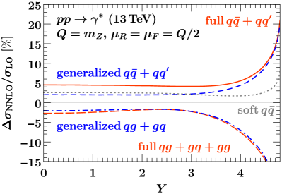
Refer to caption
Refer to caption
Refer to caption
Refer to caption
Figure S3: Top row: Generalized threshold approximation of the 𝒪(αs)𝒪subscript𝛼𝑠\mathcal{O}(\alpha_{s}) (top left) and 𝒪(αs2)𝒪superscriptsubscript𝛼𝑠2\mathcal{O}(\alpha_{s}^{2}) contribution (top right) to the Drell-Yan rapidity spectrum σdσ/(dQdY)𝜎d𝜎d𝑄d𝑌\sigma\equiv\mathrm{d}\sigma/(\mathrm{d}Q\mathrm{d}Y) at μ=Q/2𝜇𝑄2\mu=Q/2 normalized to the LO result. This is the analog of Fig. 4.
Bottom row: Convergence of the generalized and soft threshold expansions for the qq¯𝑞¯𝑞q{\bar{q}} (bottom left) and qg+gq𝑞𝑔𝑔𝑞qg+gq channels (bottom right) for μ=Q/2𝜇𝑄2\mu=Q/2. This is the analog of Fig. 5.
Refer to caption
Refer to caption
Refer to caption
Refer to caption
Figure S4: Top row: Generalized threshold approximation of the 𝒪(αs)𝒪subscript𝛼𝑠\mathcal{O}(\alpha_{s}) contribution to the ggH𝑔𝑔𝐻gg\to H rapidity spectrum σdσ/dY𝜎d𝜎d𝑌\sigma\equiv\mathrm{d}\sigma/\mathrm{d}Y at μ=mH𝜇subscript𝑚𝐻\mu=m_{H} (top left) and μ=mH/2𝜇subscript𝑚𝐻2\mu=m_{H}/2 (top right) normalized to the LO result. This is the analog of Fig. 4.
Bottom row: Convergence of the generalized and soft threshold expansions for the gg𝑔𝑔gg (bottom left) and gq+qg𝑔𝑞𝑞𝑔gq+qg channels (bottom right) for μ=mH/2𝜇subscript𝑚𝐻2\mu=m_{H}/2. This is the analog of Fig. 5.

Here, we provide additional results for the generalized threshold expansion at fixed order. The analogs of Figs. 4 and 5 for the Drell-Yan rapidity spectrum at a different scale choice μ=Q/2𝜇𝑄2\mu=Q/2 are shown in Fig. S3, and for the ggH𝑔𝑔𝐻gg\to H NLO rapidity spectrum at μ=mH𝜇subscript𝑚𝐻\mu=m_{H} and μ=mH/2𝜇subscript𝑚𝐻2\mu=m_{H}/2 in Fig. S4.

When performing any threshold expansion for different scale choices, there are several options how to treat the terms in the partonic cross section that are predicted by the running of the PDFs or αssubscript𝛼𝑠\alpha_{s}. One option is to expand these terms to the working order in the threshold expansion. This ensures that the partonic cross section has homogeneous power counting at any scale, but leaves the running of the PDFs and the coupling uncanceled beyond the working order. Another option is to threshold-expand the partonic cross section at a given reference scale and treat the running exactly. This leads to a privileged scale where the expansion was performed, but ensures the cancellation of αssubscript𝛼𝑠\alpha_{s} and PDF running to all powers (up to higher orders in αssubscript𝛼𝑠\alpha_{s}). In the following results, we choose the first option for definiteness. The difference between the two approaches could serve as a way to estimate the size of power corrections.

For Drell-Yan at μ=Q/2𝜇𝑄2\mu=Q/2, the generalized threshold expansion performs similarly well as for μ=Q𝜇𝑄\mu=Q in the main text, and again much better than the soft expansion. For ggH𝑔𝑔𝐻gg\to H, the generalized threshold expansion again performs in a manner clearly superior to the soft one. Here, the increment from the leading-power soft to the leading-power generalized approximation of the gg𝑔𝑔gg channel at NLO is roughly comparable to the piece still missing to the full result; either contribution amounts to 𝒪(20%)𝒪percent20\mathcal{O}(20\%) in units of the Born cross section. This is consistent with the expectation that for a gluon-induced process, hard central radiation plays a larger role than for Drell-Yan. The shape of the NLO contributions at large Y𝑌Y is well captured by the leading-power generalized approximation for both the gg𝑔𝑔gg and gq+qg𝑔𝑞𝑞𝑔gq+qg channel. The leading-power soft approximation for the gg𝑔𝑔gg channel (on close inspection) turns out to be off at large Y𝑌Y, and in both channels there is barely any convergence beyond leading power in the soft expansion at any Y𝑌Y.