The 2017 Failed Outburst of GX 339$-$4: Relativistic X-ray Reflection near the Black Hole Revealed by NuSTAR and Swift Spectroscopy

Abstract

We report on the spectroscopic analysis of the black hole binary GX 339$-$4 during its recent 2017–2018 outburst, observed simultaneously by the Swift and NuSTAR observatories. Although during this particular outburst the source failed to make state transitions, and despite Sun constraints during the peak luminosity, we were able to trigger four different observations sampling the evolution of the source in the hard state. We show that even for the lowest luminosity observations the NuSTAR spectra show clear signatures of X-ray reprocessing (reflection) in an accretion disk. Detailed analysis of the highest signal-to-noise spectra with our family of relativistic reflection models relxill indicates the presence of both broad and narrow reflection components. We find that a dual-lamppost model provides a superior fit when compared to the standard single lamppost plus distant neutral reflection. In the dual lamppost model two sources at different heights are placed on the rotational axis of the black hole, suggesting that the narrow component of the Fe K emission is likely to originate in regions far away in the disk, but still significantly affected by its rotational motions. Regardless of the geometry assumed, we find that the inner edge of the accretion disk reaches a few gravitational radii in all our fits, consistent with previous determinations at similar luminosity levels. This confirms a very low degree of disk truncation for this source at luminosities above $\sim 1$% Eddington. Our estimates of $R_{\mathrm{in}}$ reinforces the suggested behavior for an inner disk that approaches the inner-most regions as the luminosity increases in the hard state.

1 Introduction

The majority of stellar-mass black holes known to date are in low-mass X-ray binary systems, which are transient in nature. When in outburst, these black hole binary (BHB) systems are readily observable in X-rays, as they display a rich phenomenology in the timing and spectral domain. A typical BHB displays a fairly standard range of properties during a single outburst, otherwise spending most of its time in a quiescent state (Remillard & McClintock, 2006). Outbursts can last months to years. During a mayor cycle a single BHB can show persistent and steady jets, parsec-scale ballistic jets, quasi-periodic oscillations (QPOs) spanning 0.01–450 Hz, and transitions between spectral states broadly categorized as “hard” and “soft”, according to the overall slope of their X-ray continuum (e.g., Fender et al., 2004).

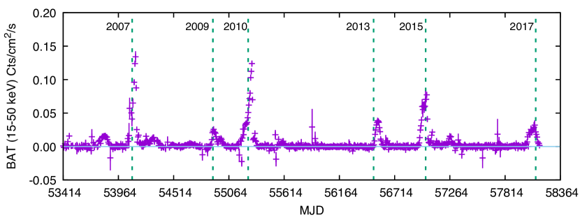
Figure 1: Swift BAT light curve (15–50 keV) covering the last six outbursts of GX 339$-$4, indicated with the vertical dashed lines. Similarly to 2013, during the 2017 outburst the source failed to transition to the soft state.

In the hard state, the X-ray spectrum of BHBs is dominated by the non-thermal emission produced by a hot ($T\sim 10^{8}-10^{9}$ K) and optically-thin ($\tau\lesssim 1-2$) plasma referred to as the corona (Haardt, 1993; Dove et al., 1997; Zdziarski et al., 2003), in clear analogy to the Sun. The origin of the corona is not well understood, but it has been associated with the base of a jet (Matt et al., 1992; Markoff et al., 2005). Recent global radiation magneto-hydrodynamic simulations suggest that this corona can form naturally in suppermassive black holes accreting at intermedium rates, i.e., 7% to 20% the Eddington rate (Jiang et al., 2019b), although a definitive theoretical prediction has not been fully produced. This coronal radiation illuminates the accretion flow producing a reflected spectrum containing many fluorescent atomic lines, absorption edges, and other spectral features (Ross & Fabian, 2005; García & Kallman, 2010). If the disk is close enough to the black hole, the reflected spectrum is distorted by the strong gravitational field (Fabian et al., 1989). Thus, the precise modeling of these signatures provides direct information on the state and composition of the material in the disk, its geometry, inclination, location of the inner radius, and ultimately the spin of the black hole (e.g., Dauser et al., 2010; Reynolds, 2014).

GX 339$-$4 is one of the most representative BHB systems known to date. Classified as a low-mass X-ray binary, it shows full outbursts every 2–3 years since its discovery (Markert et al., 1973). Even more frequent are the so called failed outbursts, during which the source fails to transition to the soft state, remaining in the hard state for the duration of a relatively shorter and less luminous cycle. In the last decade, GX 339$-$4 has undergone three full outbursts and about six failed ones.

We have previously analyzed archival data from the Rossi X-ray Timing Explorer (RXTE), tracking the evolution of the hard state (García et al., 2015), and the transition from hard to soft states (Sridhar et al., in prep.). However, the proportional counter array (PCA) onboard of RXTE offers limited spectral resolution. Meanwhile, several NuSTAR observations have covered the hard-intermediate (Fürst et al., 2016) and soft-intermediate states (Parker et al., 2016), and the hard state at low luminosities during the failed outbursts of 2013 (Fürst et al., 2015) and 2015 (Wang-Ji et al., 2018). In this paper we report on the observations of the 2017–2018 failed outburst of GX 339$-$4 , as observed simultaneously with the Neil Gehrels Swift Observatory (Swift, Gehrels et al., 2004), and NuSTAR (Harrison et al., 2013) instruments.

The remainder of the paper is organized as follows. In Section 2 we provide the details of the observations analyzed here and the reduction procedure. In Section 3 we present the main results of our spectral analysis implementing relativistic reflection models. These results are discussed in Section 4, and our main conclusions are summarized in Section 5.

2 Observations

The black hole binary GX 339$-$4 is transient X-ray source with recurrent outbursts every 2–3 years since its discovery in 1973. Figure 1 shows the hard X-ray (15–50 keV) lightcurve covering the last six outbursts observed by the Burst Alert Telescope (BAT; Barthelmy et al., 2005) instrument onboard of Swift (Gehrels et al., 2004), provided by the Hard X-ray Transit Monitor (Krimm et al., 2013). Each outburst can reach a different peak luminosity, with the source transitioning through all possible spectral accretion states (Tetarenko et al., 2016). However, in some cases the system remains in the hard state, which are often referred as failed outbursts (e.g.; Buxton et al., 2012; Belloni et al., 2013; Fürst et al., 2015). These hard-only outbursts have been observed most recently in 2009, 2013, and lastly in 2017.

Table 1: Observational Data Log for GX 339$-$4

Epoch	Telescope	Instrument	ObsId	Date	Exp (ks)	Count Rate
1	NuSTAR	FPMA/B	80302304002	2017-10-02	23	$2.1\pm 0.01$
	Swift	XRT	00032898149	2017-10-03	1	$0.4\pm 0.02$
2	NuSTAR	FPMA/B	80302304004	2017-10-25	21	$22.8\pm 0.04$
	Swift	XRT	00032898155	2017-10-23	1	$13.8\pm 0.14$
3	NuSTAR	FPMA/B	80302304005	2017-11-02	23	$16.9\pm 0.03$
	Swift	XRT	00032898160	2017-11-01	1	$11.1\pm 0.13$
4	NuSTAR	FPMA/B	80302304007	2018-01-30	32	$3.2\pm 0.01$
	Swift	XRT	00032898163	2018-01-30	1	$0.8\pm 0.03$

The last full outburst of GX 339$-$4 was observed during 2014–2015. A new outburst was reported after a brightening observed in the optical band on 2017, September (Russell et al., 2017a), followed by detections in X-rays with Swift (Gandhi et al., 2017), as well as in the radio with the Australia Telescope Compact Array (ATCA; Russell et al., 2017b). Following these detections, we triggered a series of Target of Opportunity observations from our Guest Observer program with the Nuclear Spectroscopic Telescope Array (NuSTAR; Harrison et al., 2013). Figure 2 shows the Swift BAT lightcurve around the time of the 2017 outburst, during which four NuSTAR and Swift XRT observations were performed. The first Epoch was triggered on 2017 October 2 03:40:06 UT detecting the source at $\sim 3.3$ mCrab (2–10 keV; Garcia et al., 2017). Two other observations were triggered during the rise of the outburst, until the source entered a Sun constrained period for NuSTAR (shown with the shaded region in Figure 2). The last observation took place on 2018 January 30, at which point the X-ray flux had already decreased to a level similar to that observed during Epoch 1 ($\sim 5$ mCrab, 2–10 keV). Details of all the Epochs analyzed in this paper are summarized in Table 1.

2.1 NuSTAR Extraction

The four NuSTAR observations listed in Table 1 were reduced using the standard pipeline Data Analysis Software (nustardas, v1.8.0), in combination with the caldb instrumental calibration files v20170817, which are part of heasoft v6.24. Event files were cleaned using standard filtering parameters using the nupipeline task, reducing internal background and removing data taken close to the South Atlantic Anomaly. Source products (spectra and lightcurves), backgrounds, and instrumental responses were produced for each Focal Plane Module A and B (FPMA/FPMB) using the nuproducts task. The source products were extracted from a 60” circular region centered at the position of GX 339$-$4, while background spectra were extracted from a 100” region placed at the opposite side of the same detector. Finally, spectra were binned requiring a minimum signal-to-noise of 5 per channel, and to oversample the instrument’s resolution by a factor of 3. We fitted the FPMA/B spectra in the entire energy range (3–79 keV).

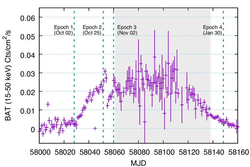
Figure 2: Closer look of the Swift BAT light curve (15–50 keV) of GX 339$-$4 during its failed 2017 outburst. The vertical dashed lines indicate the starting times of the NuSTAR observations (see Table 1). The shaded region indicates the Sun constraint period during which observations were avoided.

2.2 Swift Extraction

We made energy spectra for the four Swift XRT observations listed in Table 1 using HEASOFT v6.21 and version x20150721 of the XRT calibration files. For the observations associated with Epochs 1 and 4, XRT was in photon counting (PC) mode, and XRT was in windowed timing (WT) mode for Epochs 2 and 3. Although the count rates were lower for the PC mode observations, they were still high enough for the region at the center of the point spread function to be subject to photon pile-up, and we extracted these two spectra from an annulus with inner radius of $10^{\prime\prime}$ and an outer radius of $47^{\prime\prime}$. For the WT mode observations, the extraction region was simply a circle with a radius of $47^{\prime\prime}$. In all four cases, we subtracted background by making a spectrum from counts in an annulus around the source. We used the response matrix file swxpc0to12s6_20130101v014.rmf from the XRT calibration database and xrtmkarf with exposure maps created for each observation to produce the ancillary response file. Finally, the spectra were binned to produce the final 0.5-10 keV spectra that we used for our analysis.

3 Spectral Analysis

We analyze the time-averaged spectra from the Epochs taken with NuSTAR and Swift observatories. Although these observations are not strictly simultaneous, they were taken within 1–2 days of each other. Epochs 1 and 4 were taken at the beginning and end of the failed outburst, coincidentally at similar flux levels. Meanwhile, Epochs 2 and 3 were taken close to the peak of the outburst right before the observations were constrained by the source being too close the Sun, also with similar fluxes (see Figure 2). All the fits and statistical analysis is performed with the spectral package xspec (v12.10.0c; Arnaud, 1996).

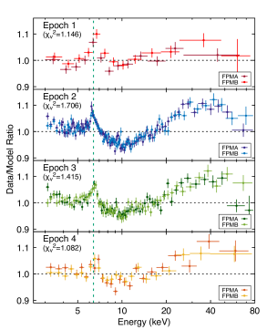
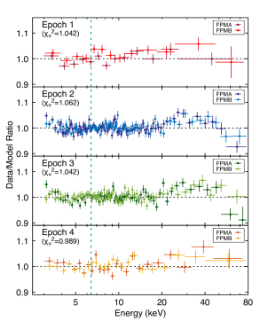
Figure 3: (left:) Data-to-model ratio plots of the NuSTAR observations fitted to an absorbed Comptonization continuum model (TBabs*nthComp). The four spectra show clear signatures of reflection, including Fe K emission near 6.4 keV (vertical dashed line), K-edge, and Compton hump. Spectra have been further rebinned to improve clarity. (right:) Ratio plots of fits including a Gaussian emission profile and a smeared edge component (TBabs*nthComp*smedge*gau). For Epochs 2 and 3, this model cannot fully reproduce the Compton hump above $\sim 20$ keV. However, the marked improvement in the fit-statistics indicates the significance of the reflection features.

3.1 Simple Description of the NuSTAR Data

We first fit a simple absorbed continuum model to all the NuSTAR data, using the thermal Comptonization model nthComp (Zdziarski et al., 1996; Życki et al., 1999). In xspec notation this model is written as TBabs*nthComp, where TBabs accounts for the neutral photoelectric absorption in the intergalactic medium, using the cross sections by Verner et al. (1996) and the cosmic abundances by Wilms et al. (2000). For simplicity, at this point we fixed the hydrogen column density to a value similar to that found in previous studies ($N_{\mathrm{H}}=6\times 10^{21}$ cm^-2, García et al., 2015; Wang-Ji et al., 2018). This parameter will be investigated later and allowed to vary freely in the final fits. The nthComp component describes the power-law like continuum produced by Comptonization of thermal disk photons in a hot gas of electrons (Zdziarski et al., 1996; Życki et al., 1999).

Figure 3 (left panels) shows ratio plots of these fits. Clear signatures of reflection are observed for all the spectra: Fe K-shell emission near 6–7 keV, Fe K-edge absorption near 10 keV, and a Compton hump peaking near 40 keV. Epochs 2 and 3 have the highest signal-to-noise and thus the most significant detection of the reflection spectrum. However, reflection is also evident in Epochs 1 and 4 despite the flux being lower by roughly an order of magnitude. The resulting reduced $\chi^{2}$ (shown in each panel) can be interpreted as an indication of the significance for the detection of the reflection signal.

A functional characterization of the reflection signatures can be achieved by fitting a Gaussian profile for the Fe K emission, and smeared edge component (smedge; Ebisawa, 1991) for the Fe K-edge. The Gaussian component is fitted with a fixed width of $\sigma=0.01$ keV, while the energy and normalization are free to vary. The smedge component was fitted with fixed index (-2.67) and width (7), while the energy and optical depth were let free to vary. The best-fit parameters are summarized in Table 2, together with an estimation of the equivalent width (EW) for the Gaussian profile, while ratio plots are shown in the right panels of Figure 3. It is evident that the inclusion of these components significantly improves the fit in all the four Epochs, with a clear decrease of the reduced chi-squared $\chi_{\nu}^{2}=\chi^{2}/\nu$ (comparing with the values quoted in the left panels of Figure 3), where $\nu$ is the number of degrees of freedom (d.o.f). Inspection of the residuals also shows that this simple functional model cannot fully reproduce the shape of the Compton hump above $\sim 20$ keV, at least the case of Epochs 2 and 3. However, given the limited signal of the data at those energies, the penalty on the fit statistics is minimal.

3.2 Analysis of the NuSTAR and Swift Data: Epochs 1 and 4

We now turn to a physically motivated model to describe the spectra of GX 339$-$4 during its 2017 failed outburst. As shown above, there are clear signatures of X-ray reprocessing in an optically-thick atmosphere. Thus, we use the reflection model relxill (García et al., 2014; Dauser et al., 2014) to fit these data. However, given their limited signal, data from Epochs 1 and 4 do not provide good constraints. In these cases, a simple reflection without any relativistic effects included (modeled with xillver, García & Kallman, 2010; García et al., 2013) already provides a good fit of the spectra. Testing a relativistic version of the same model (e.g., relxill) provides an equivalent fit, but with most parameters poorly constrained. This is likely due to an over-description of the data, given the many free parameters of the model. At most, when fitted with relativistic reflection, these data suggest that the accretion disk may be significantly truncated, as no broad component of the Fe K line can be detected. Nevertheless, it is unclear if the lack of a broad component is real, or simply due to the poor statistics of the data. Thus, we are cautious in drawing any definitive conclusions from these two spectra. Therefore, for the remainder of the analysis, we concentrate on Epochs 2 and 3, the two spectra taken during the brightest part of this outburst.

Table 2: Best-fit parameters for the final fits with relativistic reflection modeling.

Component	Parameter	Epoch 1	Epoch 2	Epoch 3	Epoch 4
TBabs	$N_{\mathrm{H}}$ ($10^{21}$ cm-2)	6	6	6	6
nthComp	$\Gamma$	$1.605\pm 0.009$	$1.565\pm 0.004$	$1.550\pm 0.005$	$1.602\pm 0.006$
nthComp	$N$ ($10^{-1}$)	$0.17\pm 0.01$	$1.4\pm 0.01$	$1.2\pm 0.01$	$0.25\pm 0.01$
Gaussian	$E$ (keV)	$6.41\pm 0.05$	$6.34\pm 0.05$	$6.53\pm 0.05$	$6.4\pm 0.1$
Gaussian	$N$ ($10^{-4}$ photons cm-2 s-1)	$0.6\pm 0.1$	$1.9\pm 0.4$	$1.9\pm 0.4$	$0.3\pm 0.2$
Smedge	$E$ (keV)	$7.2\pm 0.7$	$6.9\pm 0.1$	$6.7\pm 0.2$	$6.9\pm 0.3$
Smedge	Max $\tau$	$0.2\pm 0.1$	$0.63\pm 0.04$	$0.49\pm 0.05$	$0.40\pm 0.08$
$\chi_{\nu}^{2}$	$\cdots$	$1.042$	$1.062$	$1.042$	$0.989$
EW (eV)	$\cdots$	$74\pm 26$	$23\pm 8$	$28\pm 10$	$<36$

3.3 Analysis of the NuSTAR and Swift Data: Epochs 2 and 3

The simple fits to the NuSTAR data described above revealed the presence of clear reflection signatures. Furthermore, the inclusion of Swift XRT data shows a relatively weak excess flux in the soft bands, which can be modeled with a thermal-disk emission model (diskbb; Mitsuda et al., 1984). We have investigated these components further by following a progression of different model combinations, fitting the Swift and NuSTAR data simultaneously for Epochs 2 and 3. Ratio plots resulting from this progression of different reflection model components are shown in Figure 4. We start with a model to describe the disk emission plus the non-thermal power-law continuum with TBabs*(diskbb+nthComp). The hydrogen column is held fixed to $N_{\mathrm{H}}=6\times 10^{21}$ cm^-2, as at this point we are only interested in an overall comparison of the reflection components. In all our fits the electron temperature is pegged at its maximum allowed value of $kT_{e}=400$ keV. This parameter, which represents the temperature of the electrons in the Comptonizing corona, is constrained mostly by the cutoff of the power-law continuum at high energies, which is roughly at $E_{\mathrm{cut}}\sim 2-3(kT_{e})$. The fact that we cannot detect such a curvature means that the cutoff must at the very least at $\sim 800$ keV or above. This is consistent with the results in García et al. (2015), where we found $E_{\mathrm{cut}}\gtrsim 800$ keV for observations at $\sim 2-4$% of the Eddington luminosity. Thus, in the fits presented here, we fix the electron temperature at its upper limit of 400 keV in the nthComp component, which is also linked to the same parameter in the reflected component. Meanwhile, the disk seed-photon temperature is linked to that in the diskbb component. As in the case of the NuSTAR data alone, this model provides a decent fit to the continuum ($\chi_{\nu}^{2}$=1.64 and 1.38; for Epochs 2 and 3, respectively), but with clear residuals near 6.4 keV (reminiscent of Fe K emission) and near 30–40 keV (reminiscent of the Compton hump).

Thus, we first attempted to describe the observed residuals with a single reflection component with the xillverCp model (García & Kallman, 2010; García et al., 2013). This model produces an ionized reflection spectrum produced by the illumination of an optically-thick slab with a fixed gas density of $n_{e}=10^{15}$ cm^-3. The hard X-ray continuum is assumed to be produced by thermal Comptonization of disk photons in a hot corona, and the spectrum is calculated using the nthComp model (Zdziarski et al., 1996; Życki et al., 1999). The photon index and electron temperature are linked to those in nthComp. We further assumed a nearly neutral gas ($\log\xi=0$) and solar iron abundance ($A_{\mathrm{Fe}}=1$). Finally, the inclination is also fixed to $40$ deg, a value typically found with reflection modeling of GX 339$-$4 (García et al., 2015; Wang-Ji et al., 2018, see discussion at the end of this Section). The improvement of the fit is very dramatic, with $\Delta\chi^{2}=760$ (Epoch 2) and $435$ (Epoch 3), for only one extra d.o.f. in both cases. This clearly shows the high significance of the reflection features. However, strong residuals are still observed at high energies ($>20$ keV), and the Fe K emission appears to be over-estimated (Figure 4). Allowing the ionization parameter in the xillverCp component to vary freely does not provide a statistically significant improvement of the fit ($\chi^{2}$ only reduces by $\sim 2$). As the narrow component of the Fe K emission peaks near $6.4$ keV, this is likely driving the model toward a neutral-like reflection.

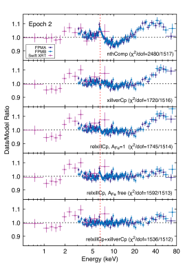
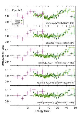
Figure 4: Data-to-model ratio plots of the Swift and NuSTAR spectra fitted with a progression of different models of increasing complexity. The models are indicated on each panel, starting with a simple absorbed Comptonization continuum model (TBabs*nthComp), and then different flavors of our reflection model relxill. Also indicated are the fit statistics for each case. Left and right panels correspond to Epochs 2 and 3, respectively. The vertical dashed line indicates 6.4 keV.

We then replaced the reflection component with its relativistic counterpart relxillCp (García et al., 2014; Dauser et al., 2014). In this model, the reflection spectrum is convolved with a general relativistic kernel to account for the distortion effects caused by the strong gravitational field near the black hole. In this variant, the emissivity of the disk is assumed to follow a power-law with radius ($\propto r^{q}$). For simplicity, we kept the emissivity index fixed to the canonical value $q=3$, which describes the profile in a standard Shakura & Sunyaev (1973) disk. The spin of the black hole is assumed to be at maximum ($a_{*}=0.998$), and again iron abundance is assumed to be solar. Only the location of the disk inner radius $R_{\mathrm{in}}$ was allowed to vary. This model provides a slightly worse fit than the one using xillverCp  and it cannot reproduce the narrow component of the Fe K emission despite pushing the inner radius to $\sim 100$ $R_{\mathrm{ISCO}}$. Most importantly, the strongest residuals at high energies remained unmodified.

In the next progression we then tried the same relativistic reflection model but allowing the iron abundance to be free. This parameter alone significantly improves the fit, with $\Delta\chi^{2}=153$ and $35$ for Epochs 2 and 3, respectively. This is mostly due to a much better fit of the high-energy part of the spectrum. The required abundance is significantly larger than the solar value ($A_{\mathrm{Fe}}\sim 5$), which is consistent with previous studies of this source (e.g., Fürst et al., 2015; García et al., 2015; Wang-Ji et al., 2018). This suggests that the specific shape of the Compton hump around 10–40 keV is mostly determined by the amount of iron in the gas. We also notice that the inner radius is significantly smaller than in the fit with fixed solar abundance ($R_{\mathrm{in}}$$\sim 2-5$ $R_{\mathrm{ISCO}}$). However, as before the narrow component of the Fe K emission is still not well modeled.

Therefore, the final progression is to include a distant reflector (i.e., not affected by relativistic effects) together with the relativistic one. This is done by using both of the relxillCp and xillverCp models, which provides the best fit of the data in this progression of models ($\chi_{\nu}^{2}$=1.016 for Epoch 2; and $\chi_{\nu}^{2}$=1.060 for Epoch 3). All the major features are well described by this model, including the broad and narrow components of the Fe K emission, the Fe K-edge, and the Compton hump.

We note that our particular choice for the inclination has a non-negligible effect in the overall fits, but it is not arbitrary. When performing the fits with free inclination, we found this parameter to be loosely constrained, but with preference for very low values (close it its lower limit of 3 deg). Low inclinations ($i\lesssim 30$ deg) can be easily ruled out by considering the most recent measurements of the mass function for this system, provided by Heida et al. (2017). Meanwhile, most recent reflection spectroscopy analyses are broadly consistent with the inclination reported for this source (e.g., García et al., 2015; Parker et al., 2016; Basak & Zdziarski, 2016), which are also well within the range derived by Zdziarski et al. (2019) on theoretical arguments. In a more extensive work, Dziełak et al. (2019) presented a systematic analysis of a high S/N spectrum for GX 339$-$4 in the hard state (specifically, the same as in Box B in García et al., 2015), using several different combinations of reflection models, arguing that results can be model dependent. However, the inclination found in their fits is either consistent with $\sim 40$ deg, or poorly constrained (see their Table 1). The largest discrepancies in the inclination derived from reflection spectroscopy is found with respect to earlier works by Miller et al. (2006) ($i=20^{+5}_{-15}$ deg), and Reis et al. (2008) ($i\lesssim 20$ deg). Both of these works fitted XMM-Newton data only (thus, no high-energy coverage), using outdated reflection models (see discussion in Section 6.1.2 of García et al., 2015). We have chosen the value of 40 deg, which was obtained in our most recent analysis of this source using the same instruments (NuSTAR and Swift), with observations taken at a relatively similar accretion state, and fitted with the same reflection models (Wang-Ji et al., 2018).

3.4 Relativistic and Distant Reflection vs. Dual-Lamppost Models

This simple progression of models discussed above indicates that both relativistic (inner regions) and non-relativistic (distant) reflection components are needed to fit these data, and that the complexity of the Fe K-edge and Compton hump region requires an iron abundance significantly larger than solar. Based on these findings, we now explore some additional and more detailed scenarios in which a lamppost geometry is assumed for the illumination of the disk (relxilllpCp). In this setup, the primary photons originate from a point source located on the spin axis at some height $h$ above the black hole. As the geometry is prescribed, the model can self-consistently calculate the reflection fraction (and reflection strength) given a set of spin, inner radius, and coronal height. Note that the reflection fraction is independent of the inclination of the reflector, as it is defined as the ratio of the coronal intensity that reaches the disk to the coronal intensity that reaches an observer at infinity directly (Dauser et al., 2016). We refer to this as Model A, which in xspec language is written as

Table 3: Best-fit parameters for Epochs 2 and 3 using a lamppost plus a distant reflection component (Model A; crabcorr*TBabs*(diskbb+relxilllpCp+xillverCp).

Component	Parameter	Epoch 2	Epoch 3
relxilllpCp	$a_{*}$	$0.998$
relxilllpCp	$i$ (deg)	$40$
relxilllpCp	$R_{\mathrm{out}}$ ($R_{\mathrm{g}})$	$1000$
relxilllpCp	$kT_{\mathrm{e}}$ (keV)	$400$
crabcorr	$\Delta\Gamma$ (XRT)	$-0.04$
TBabs	$N_{\mathrm{H}}$ ($10^{21}$ cm-2)	$6.2^{+0.8}_{-0.5}$	$6.3^{+0.4}_{-0.4}$
relxilllpCp	$h$ $(R_{\mathrm{Hor}})$	$1.6^{+0.1}_{-0.2}$	$1.6^{+0.04}_{-0.2}$
relxilllpCp	$R_{\mathrm{in}}$ ($R_{\mathrm{ISCO}})$	$<1.2$	$<1.2$
relxilllpCp	$\Gamma$	$1.37^{+0.02}_{-0.01}$	$1.37^{+0.02}_{-0.02}$
relxilllpCp	$\log\xi$ (erg cm s-1)	$4.06^{+0.01}_{-0.01}$	$4.07^{+0.02}_{-0.01}$
relxilllpCp	$A_{\mathrm{Fe}}$	$6.5^{+0.7}_{-2.7}$	$6.7^{+0.7}_{-1}$
relxilllpCp	$N$ $(10^{-2})$	$8^{+5}_{-4}$	$6^{+12}_{-2}$
xillverCp	$N$ $(10^{-3})$	$1.5^{+0.1}_{-0.2}$	$1.1^{+0.1}_{-0.2}$
diskbb	$kT_{\mathrm{in}}$ (eV)	$89^{+24}_{-10}$	$\cdots$
diskbb	$N$ $(10^{7})$	$<2$	$\cdots$
crabcorr	$\Delta\Gamma$ ($10^{-2}$, FPMB)	$2.4^{+0.6}_{-0.6}$	$0.2^{+0.3}_{-0.7}$
crabcorr	$N$ (FPMB)	$0.97^{+0.01}_{-0.01}$	$1.03^{+0.01}_{-0.02}$
crabcorr	$N$ (XRT)	$0.94^{+0.02}_{-0.02}$	$0.87^{+0.02}_{-0.02}$
Reflection Fraction	$R_{\mathrm{f}}$	$8.54$	$8.30$
Reflection Strength	$R_{\mathrm{s}}$	$2.13$	$2.23$
Photons Lost in BH	$N_{\mathrm{ph}}$ (%)	$45.8$	$42.8$
$\chi^{2}$		$1531.8$	$1569.8$
$\nu$		$1511$	$1486$
$\chi_{\nu}^{2}$		$1.014$	$1.056$

Model A:

crabcorr*TBabs*(diskbb+relxilllpCp+xillverCp)

The crabcorr model (Steiner et al., 2010), is designed to standardize detector responses to return the same normalizations and power-law slopes for the Crab, assuming as a standard the Toor & Seward (1974) fit (i.e., $\Gamma=2.1$ and $N=9.7$ photons s^-1 keV^-1). The model spectrum of each dataset is multiplied by a power law, applying both normalization and slope corrections. We keep these quantities fixed for NuSTAR FPMA ($\Delta\Gamma=0$ and $N=1$). Following Table 1 in Steiner et al. (2010), we fixed $\Delta\Gamma=-0.04$ for Swift XRT, while the rest are varied freely.

We keep the spin parameter fixed at maximum ($a_{*}=0.998$) to allow for the maximum possible disk truncation. We have found through several tests that the particular choice of the spin value does not significantly influence the overall results. In general, lower spin values provide a marginally worse fit (e.g., $\Delta\chi^{2}\sim 4$ if $a_{*}=0.5$), and both the inner radius and the height of the corona tend to decrease. Other parameters held fixed during the fit are the inclination, disk outer radius, and the electron temperature. The reflection fraction of the xillverCp component is fixed to -1 such that no other continuum is added to the model. All the parameters associated with this fit are summarized in Table 3. The quality of the fit using Model A on Epochs 2 and 3 is equivalent to that in the last iteration of the progression of models shown in the previous Section. The model requires that the primary source be placed very close to the black hole ($h\sim 1.6$ $R_{\mathrm{Hor}}$, where $R_{\mathrm{Hor}}$ is the radius of the event horizon), and for the location of inner radius consistent with the ISCO. These parameters result in a fairly large reflection fraction $R_{\mathrm{f}}\sim 8$, with more than $40$% of the primary photons lost into the black hole. The top panels of Figure 5 show the different components of Model A fitted to Epochs 2 and 3, together with their respective residuals.

Table 4: Best-fit parameters for Epochs 2 and 3 using the dual-lamppost (Model B; crabcorr*TBabs*(diskbb+relxilllpCp₁+relxilllpCp₂).

Component	Parameter	Epoch 2	Epoch 3
relxilllpCp1,2	$a_{*}$	$0.998$
relxilllpCp1,2	$i$ (deg)	$40$
relxilllpCp1,2	$R_{\mathrm{out}}$ ($R_{\mathrm{g}})$	$1000$
relxilllpCp1,2	$kT_{\mathrm{e}}$ (keV)	$400$
crabcorr	$\Delta\Gamma$ (XRT)	$-0.04$
TBabs	$N_{\mathrm{H}}$ ($10^{21}$ cm-2)	$7.0^{+0.7}_{-0.6}$	$8^{+1}_{-1}$
relxilllpCp1	$h$ $(R_{\mathrm{Hor}})$	$2.1^{+0.4}_{-0.5}$	$2.2^{+0.1}_{-0.3}$
relxilllpCp1	$R_{\mathrm{in}}$ ($R_{\mathrm{ISCO}})$	$<1.9$	$<4.5$
relxilllpCp1	$\Gamma$	$1.50^{+0.04}_{-0.01}$	$1.50^{+0.01}_{-0.07}$
relxilllpCp1	$\log\xi$ (erg cm s-1)	$3.90^{+0.09}_{-0.09}$	$4.03^{+0.02}_{-0.05}$
relxilllpCp1	$A_{\mathrm{Fe}}$	$4.0^{+0.3}_{-0.5}$	$4.0^{+0.4}_{-0.8}$
relxilllpCp1	$N$ $(10^{-2})$	$1.2^{+0.8}_{-0.4}$	$1.6^{+0.2}_{-0.3}$
relxilllpCp2	$h$ $(R_{\mathrm{g}})$	$503^{+160}_{-105}$	$>765$
relxilllpCp2	$N$ $(10^{-3})$	$4.5^{+0.9}_{-1.5}$	$2.9^{+0.2}_{-0.4}$
diskbb	$kT_{\mathrm{in}}$ (eV)	$90^{+19}_{-17}$	$84^{+35}_{-31}$
diskbb	$N$ $(10^{6})$	$4^{+12}_{-4}$	$<184$
crabcorr	$\Delta\Gamma$ ($10^{-2}$, FPMB)	$2.5^{+0.6}_{-0.6}$	$0.1^{+0.7}_{-0.7}$
crabcorr	$N$ (FPMB)	$0.97^{+0.01}_{-0.01}$	$1.02^{+0.02}_{-0.01}$
crabcorr	$N$ (XRT)	$0.93^{+0.02}_{-0.02}$	$0.87^{+0.02}_{-0.02}$
Reflection Fraction	$R_{\mathrm{f}}$	$4.35$	$4.77$
Reflection Strength	$R_{\mathrm{s}}$	$2.04$	$2.14$
Photons Lost in BH	$N_{\mathrm{ph}}$ (%)	$29.4$	$32.4$
$\chi^{2}$		$1502.1$	$1532.7$
$\nu$		$1510$	$1483$
$\chi_{\nu}^{2}$		$0.995$	$1.034$

Despite the success of Model A, careful inspection of Figure 5 shows some structure in the residuals near the Fe K region, which suggests that the narrow component of the iron emission is perhaps more complex than the one produced by a distant reflector. We have thus tried an additional fit, in which the xillverCp component is replaced by a second lamppost, one situated at a larger height than the first one. We refer to this as Model B, written as

Model B:

crabcorr*TBabs*(diskbb+relxilllpCp₁+relxilllpCp₂)

In this Model B, all the parameters of the second lamppost are tied to the first one, except for the height and the normalization. As in the case of the distant reflection, we set the reflection fraction of the second lamppost to -1, such that only one continuum is included by the model (via the first lamppost). Furthermore, given the poor constraint on the inner radius, and to ensure that the second lamppost only provides reflection from farther away in the disk, we assume that $R_{\mathrm{in}}$₂ is equal to the height of the lamppost (this implies that the second lamppost only produces reflection in a disk with a much larger inner radius). With only one extra d.o.f., the dual lamppost (Model B) provides significantly better fit statistics ($\Delta\chi^{2}=30$ for Epoch 2, and $\Delta\chi^{2}=37$ for Epoch 3). The best fit parameters are summarized in Table 4, while the model components and residuals are shown the bottom panels of Figure 5.

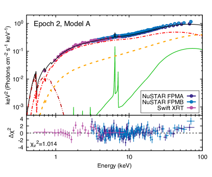
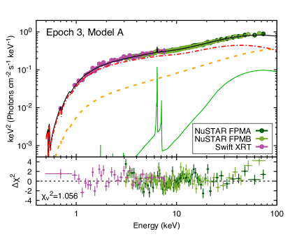
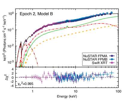
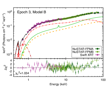
Figure 5: Analysis of the spectra from Epochs 2 and 3 (left and right), using relativistic reflection in a lamppost geometry for the inner reflection and a non-relativistic, distant reflector (Model A, top panels); or a second lamppost located higher in the rotational axis (Model B, bottom panels). The individual model components are shown: total model (solid black), coronal emission (nthComp; dashed orange), disk emission (diskbb; dot-dot dashed red), relativistic reflection from a lamppost (relxilllpCp; dot-dashed red), and distant reflection or second lamppost (xillverCp or relxilllpCp; solid green). The bottom sub-panels show the residuals of each fit, with the resulting $\chi^{2}_{\nu}$ indicated in each case.

4 Discussion

The spectral fits detailed in the previous Sections reveal several important aspects of the evolution of GX 339$-$4 in the early stages of its frequent outbursts. We find that even at very low accretion rates, such as those observed during Epochs 1 and 4 ($\sim 0.2$% $L_{\mathrm{Edd}}$), the spectrum observed by NuSTAR shows clear hallmarks of X-ray reprocessing in an optically-thick medium, likely the accretion disk. These include Fe K emission near 6.4 keV, a smeared Fe K-edge at $\sim 7-10$ keV, and possibly a Compton hump at higher energies (20–40 keV). Given the limited signal of these low-luminosity observations, we cannot confidently determine the width of the Fe K emission, nor constrain the disk inner radius. Interestingly, the equivalent width of the Fe K emission measured in Epochs 1 and 4 ($74\pm 26$ eV and $<36$ eV) are larger than in Epochs 2 and 3 ($23\pm 8$ eV and $28\pm 10$ eV), contrary to the expectation of a stronger emission if the inner accretion disk moves inward when the luminosity increases. This is likely due to the fact that the smedge component can be unphysically large, resulting in strong degeneracies. However, the EW measured in Epoch 1 agrees well with the value of $73^{+18}_{-14}$ eV previously measured by Tomsick et al. (2009) with Suzaku data taken at a similar luminosity level.

Testing different types of reflection models on the highest luminosity observations (Epochs 2 and 3), we find that both relativistic (broad) and non-relativistic (narrow) components are strongly required to fit the data. Our two main fits are then based on these findings. Model A includes relativistic reflection from the inner accretion disk invoking a lamppost geometry, as well as a non-relativistic reflection component assumed to be produced much farther, possibly in the outer disk or the surface of the companion star. Meanwhile, Model B replaces the non-relativistic reflection for a second lamppost, which is placed at a much larger height, and thus preferentially illuminates larger radii in the disk, producing a narrower Fe K emission than the lamppost located close to the black hole.

While both Models A and B reproduce the data well, Model B yields better fit statistics, with $\chi_{\nu}^{2}$=0.995 for Epoch 2, which represents an improvement of $\Delta\chi^{2}=30$ for only one extra d.o.f. Fits to Epoch 3 also resulted in a preference for Model B ($\chi_{\nu}^{2}$=1.034; $\Delta\chi^{2}=37$). Most of this improvement comes from a better fit of the narrow component of the Fe K emission, which suggest that this narrow component could in fact originate in a region of the disk at sufficiently large radii such that relativistic effects are largely negligible, but close enough to still be affected by the rotational motion of the disk. Similar complexity has been seen in the narrow Fe K component in the black hole binary candidate MAXI J1535$-$571, independently by both NuSTAR (Xu et al., 2018), and NICER (Miller et al., 2018), and also possibly in the black hole binary candidate MAXI J1820+070 (Buisson et al. in prep).

Although the lamppost is a highly idealized geometry, it provides a good description of the observed X-ray spectrum, and allows for the determination of several key parameters, such as how close to the black hole the primary source is located, and the exact relative strength of the direct and reflected components (i.e., the reflection fraction). Furthermore, the dual lamppost description (Model B) is not only superior in terms of the fit statistics, but also in the overall quantities recovered by the fit. The height of the source is slightly higher in Model B, which implies a more reasonable reflection fraction ($R_{\mathrm{f}}\sim 4-5$ vs $8-9$ for Model A), which reduces the fraction of photons lost into the black hole from $\sim 40$% to $\sim 30$%, relaxing the high luminosity implied for the primary source. We notice that the photon index increases from $\Gamma=1.37$ to $1.5$ between Models A and B, with the latter value being more consistent with values reported in previous analysis (e.g., Fürst et al., 2015; García et al., 2015; Wang-Ji et al., 2018).

The ionization parameter, which is proportional to the ratio of the incident flux to the gas density ($\xi=4\pi F_{x}/n_{e}$), is found to be significantly larger than in previous studies at similar accretion states (e.g., Fürst et al., 2015; García et al., 2015; Wang-Ji et al., 2018). This is true for both Models A and B, and in both Epochs 2 and 3. Taking the case of Epoch 2, the 2–10 keV observed flux is comparable to that in Obs. 1 (2015) of Wang-Ji et al. (2018), who reported $\log\xi\sim 3.3$, while we find $\log\xi\sim 4$. Assuming that the fluxes in the two observations are in fact identical, the difference can only be attributed to a change in the density of the disk’s atmosphere by a factor of $\sim 5$. This difference does not seem implausible, given the intrinsic turbulent nature of accretion disks (e.g., Kadowaki et al., 2018), and how strongly magnetic fields can affect the surface density in the accretion disk (e.g., Jiang et al., 2019b).

In the case of Epoch 3, we found that when using Model A the thermal disk component (diskbb) is not statistically required, as it produces virtually no change in the goodness of the fit, and the model parameters are unconstrained. The situation is different when using Model B, in which case we found an improvement of $\Delta\chi^{2}=8$ when adding the thermal disk component. This is likely due to the smaller reflection fraction, which lowers the reflected continuum and makes the disk emission more obvious in the fit. Nevertheless, we notice that this spectral feature is not very prominent, and its origin cannot be fully determined. For example, García et al. (2016) showed that when the density in the reflector is over $\sim 10^{17}$ cm^-3 there is an enhancement of reflected flux at soft energies. As mentioned above, the relatively large ionization parameter indicates the possibility of an also large density in the accretion disk, which could then explain the soft excess observed in the spectra. As we discuss next, these high-density effects can also have important consequences in the abundance of iron derived form reflection spectroscopy.

The iron abundance for Model A is constrained at more than 6 times its Solar value, while for Model B (dual lamppost) it is found to be $\sim 4$ times solar. Both of these results are consistent with our previous analysis of RXTE PCA (García et al., 2015) and NuSTAR data (Wang-Ji et al., 2018). However, Jiang et al. (2019a) has recently demonstrated that by implementing new reflection models calculated at high densities the requirement for the disk thermal emission vanishes, and the recovered iron abundance is more consistent with the Solar value. Since these high density models are still under development, and given that all the other parameters remain unchanged in the analysis of Jiang et al. (2019a), we deferred their application to these data for a future publication.

It is important to notice that both of these models constrain the inner radius to be very close to the ISCO radius, specifically $R_{\mathrm{in}}$$<1.2$ $R_{\mathrm{ISCO}}$ for Model A (distant reflector), and $R_{\mathrm{in}}$$=2-5$ $R_{\mathrm{ISCO}}$ for Model B (dual lamppost). Figure 6 shows a comparison our results with several other inner radius measurements of GX 339$-$4 with reflection spectroscopy. The values of $R_{\mathrm{in}}$ (in units of gravitational radius $R_{g}=GM/c^{2}$) are plotted as a function of the Eddington scaled luminosity $L_{\mathrm{Edd}}$$=1.25\times 10^{39}$ erg s^-1 (assuming a distance of $D=8$ kpc and a black hole mass of $M=10$ $M_{\odot}$; Zdziarski et al., 2004). The results from our analysis of the 2017 failed outburst data are in good agreement with the overall trend of a decreasing inner radius with increasing luminosity in the hard state. Furthermore, the trend observed in Figure 6 indicates that the inner accretion disk appears to be relatively close to the ISCO radius early on in the outburst, reaching few times $R_{\mathrm{ISCO}}$ at $\sim 1$% $L_{\mathrm{Edd}}$. Interestingly, this trend appears to be independent of whether the source was observed during the rise or the decay of the outburst, and on whether the outburst itself was full (i.e., the source went through state transitions), or a failed one (such as the one analyzed here).

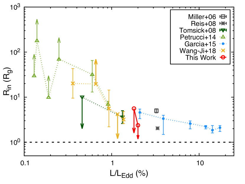
Figure 6: Comparison of the inner radius values derived from reflection spectroscopy as a function of the Eddington-scaled luminosity for the hard state of GX 339$-$4. Reported values include those from analysis of XMM-Newton MOS (Miller et al., 2006; Reis et al., 2008), Suzaku (Tomsick et al., 2008; Petrucci et al., 2014), RXTE PCA (García et al., 2015), and Swift+NuSTAR (Wang-Ji et al., 2018). Our values derived from the 2017 Swift+NuSTAR data are in good agreement with the observed correlation between $R_{\mathrm{in}}$ and the source luminosity.

5 Conclusions

The black hole binary system GX 339$-$4 goes into outburst regularly, with a full outburst typically observed every 2–3 years (Tetarenko et al., 2016). In this paper we have presented a reflection spectroscopy analysis of the X-ray spectrum of GX 339$-$4 as observed by NuSTAR and Swift during the 2017 failed outburst. We triggered 3 observations on the rise in the hard state. The source reached $\sim 50$ mCrab (2–10 keV), before observations were restricted due to Sun constraint during December 2017. One more observation done at the end of January 2018 showed that the source did not transition to the soft state, and it was already on the decay to quiescence.

The NuSTAR spectra from our observations show clear signatures of X-ray reflection from an optically-thick accretion disk (i.e., Fe K emission, K-edge, and Compton hump). Detailed spectroscopic analysis for the two brightest observations revealed the need for a relativistically broadened reflection component, as well as a narrow and likely more distant reflection component; in addition to a non-thermal (power-law like) continuum, and weak thermal disk emission. Our analysis focuses on two main fits, both including a relativistic reflection model using the lamppost geometry.

The dual-lamppost description is preferred over the single lamppost plus a simple distant reflector, based on a relatively significant improvement of the fit statistics of the two highest S/N spectra in our sample. The second lamppost, which is situated at a much larger height than the first, provides a better fit to the narrow component of the Fe K emission. This picture is consistent with a corona that has a certain vertical dimension and is capable of illuminating the outer regions of the accretion disk. Meanwhile, we do not detect any changes in the coronal emission, as the slope of the non-thermal continuum is consistent among the four observations analyzed here, and no high-energy cutoff can be detected (and thus fixed in our fits).

The results from these fits are in good agreement with our recent analysis done with the same reflection models on NuSTAR and Swift data from the previous 2015 and 2013 outbursts (Wang-Ji et al., 2018), as well as with those derived from the analysis of RXTE observations (García et al., 2015). Particularly, we find that the inner radius of the accretion disk is close to the ISCO in the two models adopted here. Most importantly, our measurements are fully consistent with the observed trend of $R_{\mathrm{in}}$ decreasing as the luminosity in the hard state increases. The present analysis shows that the inner disk must be close to the ISCO early on during the outburst, and that it is typically within a few ISCO radii for luminosities of $\sim 1$% Eddington. Crucially, this trend has been constructed with data provided by different observatories such as Suzaku, Swift, RXTE, and NuSTAR; with observations taken during full and failed outbursts, and during both the rise and decay phases of the hard state evolution. This implies that the state transitions between hard and soft states are unlikely to be triggered by changes in the location of the inner accretion disk, but rather by other mechanisms. Future and continuous monitoring of this and other black hole transient sources will provide valuable new insights into the accretion physics of these systems.

References

- Arnaud (1996) Arnaud, K. A. 1996, in Astronomical Society of the Pacific Conference Series, Vol. 101, Astronomical Data Analysis Software and Systems V, ed. G. H. Jacoby & J. Barnes, 17
- Barthelmy et al. (2005) Barthelmy, S. D., Barbier, L. M., Cummings, J. R., et al. 2005, Space Sci. Rev., 120, 143, doi: 10.1007/s11214-005-5096-3
- Basak & Zdziarski (2016) Basak, R., & Zdziarski, A. A. 2016, MNRAS, 458, 2199, doi: 10.1093/mnras/stw420
- Belloni et al. (2013) Belloni, T. M., Motta, S., & Casella, P. 2013, The Astronomer’s Telegram, 5417
- Buxton et al. (2012) Buxton, M. M., Bailyn, C. D., Capelo, H. L., et al. 2012, AJ, 143, 130, doi: 10.1088/0004-6256/143/6/130
- Dauser et al. (2014) Dauser, T., García, J., Parker, M. L., Fabian, A. C., & Wilms, J. 2014, MNRAS, 444, L100, doi: 10.1093/mnrasl/slu125
- Dauser et al. (2016) Dauser, T., García, J., Walton, D. J., et al. 2016, A&A, 590, A76, doi: 10.1051/0004-6361/201628135
- Dauser et al. (2010) Dauser, T., Wilms, J., Reynolds, C. S., & Brenneman, L. W. 2010, MNRAS, 409, 1534, doi: 10.1111/j.1365-2966.2010.17393.x
- Dove et al. (1997) Dove, J. B., Wilms, J., Maisack, M., & Begelman, M. C. 1997, ApJ, 487, 759, doi: 10.1086/304647
- Dziełak et al. (2019) Dziełak, M. A., Zdziarski, A. A., Szanecki, M., et al. 2019, MNRAS, 485, 3845, doi: 10.1093/mnras/stz668
- Ebisawa (1991) Ebisawa, K. 1991, PhD thesis, Insititute of Space and Astronautical Science/Japan Aerospace Exploration Agency
- Fabian et al. (1989) Fabian, A. C., Rees, M. J., Stella, L., & White, N. E. 1989, MNRAS, 238, 729
- Fender et al. (2004) Fender, R. P., Belloni, T. M., & Gallo, E. 2004, MNRAS, 355, 1105, doi: 10.1111/j.1365-2966.2004.08384.x
- Fürst et al. (2015) Fürst, F., Nowak, M. A., Tomsick, J. A., et al. 2015, ApJ, 808, 122, doi: 10.1088/0004-637X/808/2/122
- Fürst et al. (2016) Fürst, F., Grinberg, V., Tomsick, J. A., et al. 2016, ApJ, 828, 34, doi: 10.3847/0004-637X/828/1/34
- Gandhi et al. (2017) Gandhi, P., Altamirano, D., Russell, D. M., et al. 2017, The Astronomer’s Telegram, 10798
- García et al. (2013) García, J., Dauser, T., Reynolds, C. S., et al. 2013, ApJ, 768, 146, doi: 10.1088/0004-637X/768/2/146
- García & Kallman (2010) García, J., & Kallman, T. R. 2010, ApJ, 718, 695, doi: 10.1088/0004-637X/718/2/695
- García et al. (2014) García, J., Dauser, T., Lohfink, A., et al. 2014, ApJ, 782, 76, doi: 10.1088/0004-637X/782/2/76
- García et al. (2016) García, J. A., Fabian, A. C., Kallman, T. R., et al. 2016, MNRAS, 462, 751, doi: 10.1093/mnras/stw1696
- Garcia et al. (2018) Garcia, J. A., Grefenstette, B., Harrison, F., Tomsick, J., & Miyasaka, H. 2018, The Astronomer’s Telegram, 12322
- García et al. (2015) García, J. A., Steiner, J. F., McClintock, J. E., et al. 2015, ApJ, 813, 84, doi: 10.1088/0004-637X/813/2/84
- Garcia et al. (2017) Garcia, J. A., Harrison, F., Tomsick, J., et al. 2017, The Astronomer’s Telegram, 10825
- Gehrels et al. (2004) Gehrels, N., Chincarini, G., Giommi, P., et al. 2004, ApJ, 611, 1005, doi: 10.1086/422091
- Haardt (1993) Haardt, F. 1993, ApJ, 413, 680, doi: 10.1086/173036
- Harrison et al. (2013) Harrison, F. A., Craig, W. W., Christensen, F. E., et al. 2013, ApJ, 770, 103, doi: 10.1088/0004-637X/770/2/103
- Heida et al. (2017) Heida, M., Jonker, P. G., Torres, M. A. P., & Chiavassa, A. 2017, ApJ, 846, 132, doi: 10.3847/1538-4357/aa85df
- Jiang et al. (2019a) Jiang, J., Fabian, A. C., Wang, J., et al. 2019a, MNRAS, 484, 1972, doi: 10.1093/mnras/stz095
- Jiang et al. (2019b) Jiang, Y.-F., Blaes, O., Stone, J., & Davis, S. W. 2019b, arXiv e-prints. https://arxiv.org/abs/1904.01674
- Kadowaki et al. (2018) Kadowaki, L. H. S., De Gouveia Dal Pino, E. M., & Stone, J. M. 2018, ApJ, 864, 52, doi: 10.3847/1538-4357/aad4ff
- Kirsch et al. (2005) Kirsch, M. G., Briel, U. G., Burrows, D., et al. 2005, in Society of Photo-Optical Instrumentation Engineers (SPIE) Conference Series, Vol. 5898, UV, X-Ray, and Gamma-Ray Space Instrumentation for Astronomy XIV, ed. O. H. W. Siegmund, 22–33
- Krimm et al. (2013) Krimm, H. A., Holland, S. T., Corbet, R. H. D., et al. 2013, ApJS, 209, 14, doi: 10.1088/0067-0049/209/1/14
- Kubota et al. (1998) Kubota, A., Tanaka, Y., Makishima, K., et al. 1998, PASJ, 50, 667, doi: 10.1093/pasj/50.6.667
- Markert et al. (1973) Markert, T. H., Canizares, C. R., Clark, G. W., et al. 1973, ApJ, 184, L67, doi: 10.1086/181290
- Markoff et al. (2005) Markoff, S., Nowak, M. A., & Wilms, J. 2005, 635, 1203
- Matt et al. (1992) Matt, G., Perola, G. C., Piro, L., & Stella, L. 1992, A&A, 257, 63
- Miller et al. (2006) Miller, J. M., Homan, J., Steeghs, D., et al. 2006, ApJ, 653, 525, doi: 10.1086/508644
- Miller et al. (2018) Miller, J. M., Gendreau, K., Ludlam, R. M., et al. 2018, ApJ, 860, L28, doi: 10.3847/2041-8213/aacc61
- Mitsuda et al. (1984) Mitsuda, K., Inoue, H., Koyama, K., et al. 1984, PASJ, 36, 741
- Parker et al. (2016) Parker, M. L., Tomsick, J. A., Kennea, J. A., et al. 2016, ApJ, 821, L6, doi: 10.3847/2041-8205/821/1/L6
- Petrucci et al. (2014) Petrucci, P.-O., Cabanac, C., Corbel, S., Koerding, E., & Fender, R. 2014, A&A, 564, A37, doi: 10.1051/0004-6361/201322268
- Reis et al. (2008) Reis, R. C., Fabian, A. C., Ross, R. R., et al. 2008, MNRAS, 387, 1489, doi: 10.1111/j.1365-2966.2008.13358.x
- Remillard & McClintock (2006) Remillard, R. A., & McClintock, J. E. 2006, ARA&A, 44, 49, doi: 10.1146/annurev.astro.44.051905.092532
- Reynolds (2014) Reynolds, C. S. 2014, Space Sci. Rev., 183, 277, doi: 10.1007/s11214-013-0006-6
- Ross & Fabian (2005) Ross, R. R., & Fabian, A. C. 2005, MNRAS, 358, 211, doi: 10.1111/j.1365-2966.2005.08797.x
- Russell et al. (2017a) Russell, D. M., Lewis, F., & Gandhi, P. 2017a, The Astronomer’s Telegram, 10797
- Russell et al. (2017b) Russell, T. D., Tetarenko, A. J., Sivakoff, G. R., & Miller-Jones, J. C. A. 2017b, The Astronomer’s Telegram, 10808
- Shakura & Sunyaev (1973) Shakura, N. I., & Sunyaev, R. A. 1973, A&A, 24, 337
- Steiner et al. (2010) Steiner, J. F., McClintock, J. E., Remillard, R. A., et al. 2010, ApJ, 718, L117, doi: 10.1088/2041-8205/718/2/L117
- Tetarenko et al. (2016) Tetarenko, B. E., Sivakoff, G. R., Heinke, C. O., & Gladstone, J. C. 2016, ApJS, 222, 15, doi: 10.3847/0067-0049/222/2/15
- Tomsick et al. (2009) Tomsick, J. A., Yamaoka, K., Corbel, S., et al. 2009, ApJ, 707, L87, doi: 10.1088/0004-637X/707/1/L87
- Tomsick et al. (2008) Tomsick, J. A., Kalemci, E., Kaaret, P., et al. 2008, ApJ, 680, 593, doi: 10.1086/587797
- Toor & Seward (1974) Toor, A., & Seward, F. D. 1974, AJ, 79, 995, doi: 10.1086/111643
- Verner et al. (1996) Verner, D. A., Ferland, G. J., Korista, K. T., & Yakovlev, D. G. 1996, ApJ, 465, 487, doi: 10.1086/177435
- Wang-Ji et al. (2018) Wang-Ji, J., García, J. A., Steiner, J. F., et al. 2018, ApJ, 855, 61, doi: 10.3847/1538-4357/aaa974
- Wilms et al. (2000) Wilms, J., Allen, A., & McCray, R. 2000, ApJ, 542, 914, doi: 10.1086/317016
- Xu et al. (2018) Xu, Y., Harrison, F. A., García, J. A., et al. 2018, ApJ, 852, L34, doi: 10.3847/2041-8213/aaa4b2
- Zdziarski et al. (2004) Zdziarski, A. A., Gierliński, M., Mikołajewska, J., et al. 2004, MNRAS, 351, 791, doi: 10.1111/j.1365-2966.2004.07830.x
- Zdziarski et al. (1996) Zdziarski, A. A., Johnson, W. N., & Magdziarz, P. 1996, MNRAS, 283, 193, doi: 10.1093/mnras/283.1.193
- Zdziarski et al. (2003) Zdziarski, A. A., Lubiński, P., Gilfanov, M., & Revnivtsev, M. 2003, MNRAS, 342, 355, doi: 10.1046/j.1365-8711.2003.06556.x
- Zdziarski et al. (2019) Zdziarski, A. A., Ziółkowski, J., & Mikołajewska, J. 2019, arXiv e-prints, arXiv:1904.07803. https://arxiv.org/abs/1904.07803
- Życki et al. (1999) Życki, P. T., Done, C., & Smith, D. A. 1999, MNRAS, 309, 561, doi: 10.1046/j.1365-8711.1999.02885.x