Deterministic Completion of Rectangular Matrices
Using Asymmetric Ramanujan Graphs:
Exact and Stable Recovery

Abstract

In this paper we study the matrix completion problem: Suppose $X\in{\mathbb{R}}^{n_{r}\times n_{c}}$ is unknown except for a known upper bound $r$ on its rank. By measuring a small number $m\ll n_{r}n_{c}$ of elements of $X$, is it possible to recover $X$ exactly with noise-free measurements, or to construct a good approximation of $X$ with noisy measurements? Existing solutions to these problems involve sampling the elements uniformly and at random, and can guarantee exact recovery of the unknown matrix only with high probability. In this paper, we present a deterministic sampling method for matrix completion. We achieve this by choosing the sampling set as the edge set of an asymmetric Ramanujan bigraph, and constrained nuclear norm minimization is the recovery method. Specifically, we derive sufficient conditions under which the unknown matrix is completed exactly with noise-free measurements, and is approximately completed with noisy measurements, which we call “stable” completion. This is in contrast to “robust” completion where it is assumed that measurement errors occur only in a few locations. We show that the same conditions that suffice for exact completion under noise-free measurements also suffice to permit an accurate, though not exact, reconstruction with noisy measurements.

The conditions derived here are only sufficient and more restrictive than random sampling. To study how close they are to being necessary, we conducted numerical simulations on randomly generated low rank matrices, using the LPS families of Ramanujan graphs. These simulations demonstrate two facts: (i) In order to achieve exact completion, it appears sufficient to choose the degree $d$ of the Ramanujan graph to be $\geq 3r$. (ii) There is a “phase transition,” whereby the likelihood of success suddenly drops from 100% to 0% if the rank is increased by just one or two beyond a critical value. The phase transition phenomenon is well-known and well-studied in vector recovery using $\ell_{1}$-norm minimization. However, it is less studied in matrix completion and nuclear norm minimization, and not much understood.

1 Introduction

1.1 General Statement

Compressed sensing refers to the recovery of high-dimensional but low-complexity objects from a small number of linear measurements. Recovery of sparse (or nearly sparse) vectors, and recovery of high-dimensional but low-rank matrices are the two most popular applications of compressed sensing. The object of study in the present paper is the matrix completion problem, which is a special case of low-rank matrix recovery. The matrix completion problem has been receiving attention due to its application to different areas such as rating systems or recommendation engines (also known as the “Netflix problem” [1], sensor localization, structure from motion [2], and quantum tomography [3, 4, 5, 6, 7, 8, 9]. In recommendation engines, the rows represent the products, ranging from the hundreds to the thousands, while the columns represent customers, ranging into the millions. In the community working on recommendation engines, it is believed, rightly or wrongly, that each customer uses no more than ten to fifteen features to make a selection; consequently, the matrix with all entries of customer preferences has rank no more than fifteen. In sensor localization, the idea is to infer the pairwise 3-D distance between $l$ different points, from measuring only a few pairwise distances. It can be shown that, no matter how large the number $l$ of points is, this matrix has rank no more than five. In quantum tomography, the dimensions can be huge, $2^{2^{n}}$ where $n$ is the number of qubits, but the matrix often has rank one or two. An excellent survey of the matrix completion problem can be found in [10].

1.2 Problem Definition

The matrix completion problem can be stated formally as follows: Suppose $X\in{\mathbb{R}}^{n_{r}\times n_{c}}$ is an unknown matrix that we wish to recover whose rank is bounded by a known integer $r$. Let $[n]$ denote the set $\{1,\ldots,n\}$ for each integer $n$. In the matrix completion problem, a set $\Omega\subseteq[n_{r}]\times[n_{c}]$ is specified, known as the sample set or measurement set. To be specific, suppose $\Omega=\{(i_{1},j_{1}),\ldots,(i_{m},j_{m})\}$, where $|\Omega|=m$ is the total number of samples. We are able to observe the values of the unknown matrix $X$ at the locations in the set $\Omega$, either with or without noise. In the noise-free case, the measurements consist of $X_{i,j}$ for all $(i,j)\in\Omega$. Equivalently, the measured matrix $S$ can be expressed as the Hadamard product $E_{\Omega}\circ X$ where $E_{\Omega}\in\{0,1\}^{n_{r}\times n_{c}}$ is defined by

$$(E_{\Omega})_{ij}=\left\{\begin{array}[]{ll}1&\mbox{if }(i,j)\in\Omega,\\ 0&\mbox{if }(i,j)\not\in\Omega.\end{array}\right.$$

Note that if $X_{ij}$ happens to equal zero at some sampled location $(i,j)\in\Omega$, then the measured matrix $S:=E_{\Omega}\circ X$ will also equal zero at the same location. However, at the unsampled locations, $S=E_{\Omega}\circ X$ will always equal zero. In the exact matrix completion problem, the objective is to recover the unknown matrix $X$ exactly from $E_{\Omega}\circ X$. In the case of noisy measurements, the data available to the learner consists of $E_{\Omega}\circ X+{\cal W}$, where ${\cal W}$ is the measurement noise. In this case it is possible to make a distinction between two cases. In the robust matrix completion problem, it is assumed that the noise matrix ${\cal W}$ is sparse, that is, ${\cal W}_{ij}=0$ for all but a small number of pairs $(i,j)$. The objective is still to recover $X$ exactly. In the stable matrix completion problem, there are no assumptions on the number of nonzero elements of ${\cal W}$, but there is a known upper bound $\epsilon$ on the Frobenius norm of ${\cal W}$. In this case, exact recovery of $X$ may not be possible. Therefore, in stable matrix completion, the aim is to construct an accurate approximation to $X$.

In the case of noise-free measurements, one possible approach to the matrix completion problem is to set

$$\hat{X}=\operatornamewithlimits{argmin}_{Z\in{\mathbb{R}}^{n_{r}\times n_{c}}}{\rm{rank}}(Z)\mbox{ s.t. }E_{\Omega}\circ Z=E_{\Omega}\circ X.$$ (1)

The above problem is a special case of minimizing the rank of an unknown matrix subject to linear constraints, and is therefore NP-hard [11]. Since the problem is NP-hard, a logical approach is to replace the rank function by its convex relaxation, which is the nuclear norm, or the sum of the singular values of a matrix, as shown in [12]. Therefore the convex relaxation of (1) is

$$\hat{X}:=\operatornamewithlimits{argmin}_{Z\in{\mathbb{R}}^{n_{r}\times n_{c}}}\|Z\|_{N}\mbox{ s.t. }E_{\Omega}\circ Z=E_{\Omega}\circ X.$$ (2)

In the case of sparse noisy measurements, the above formulation can be still used (more in the section on literature review below). In the case of unstructured noisy measurements, let us define $X_{\cal W}=X+{\cal W}$, so that the noise-corrupted measurement consists of the Hadamard product $E_{\Omega}\circ X_{\cal W}$. In this case, as suggested in [13], (2) can be modified to

$$\hat{X}:=\operatornamewithlimits{argmin}_{Z\in{\mathbb{R}}^{n_{r}\times n_{c}}}\|Z\|_{N}\mbox{ s.t. }\|E_{\Omega}\circ Z-E_{\Omega}\circ X_{\cal W}\|_{F}\leq\epsilon$$ (3)

where $\epsilon$ is a known upper bound on the Frobenius norm of the measurement error matrix ${\cal W}$. For instance, if ${\cal W}$ represents Gaussian noise with known characteristics, a bound on its Frobenius norm can be derived with a specified prior probability.

1.3 Contributions of the Present Paper

In the literature to date, most of the papers assume that the sample set $\Omega$ is chosen at random from $[n_{r}]\times[n_{c}]$, either without replacement as in [1, 14], or with replacement [15]. The authors are aware of only a handful of papers [16, 17, 18, 19, 20] in which a deterministic procedure is suggested for choosing the sample set $\Omega$. In [16, 17], the sample set $\Omega$ is chosen as the edge set of a Ramanujan graph. (This concept is defined below). Other references such as [19] suggest that the sample set $\Omega$ can be viewed as the edge set of a bipartite graph, but do not explicitly take advantage of this. In [17], the authors use nuclear norm minimization as in (2), and claim to derive some sufficient conditions. However, as shown in the Appendix, there is an error in that paper. In contrast, we present a correct sufficient condition for exact matrix completion. Moreover, our method of proof carries over seamlessly to stable matrix completion, which is not studied in [17]. In [16], the approach is max-norm minimization. The results there are “universal” in that they do not involve the coherence parameter of the unknown matrix $X$ (defined below), and also apply to the case where the elements are sampled with a nonuniform probability. The present authors have improved upon those bounds by a factor of two; see [21]. These improvements are achieved through modifying the so-called “expander mixing lemma” for bipartite graphs, which is independent interest. However, due to space limitations, the max norm minimization approach to exact matrix completion is not discussed in this paper.

2 Literature Review

There are two approaches to choosing the sample set $\Omega$, namely probabilistic and deterministic. In the probabilistic approach the elements of $\Omega$ are chosen at random from $[n_{r}]\times[n_{c}]$, usually, though not always, with a uniform distribution. In this setting one can further distinguish between two distinct situations, namely sampling from $[n_{r}]\times[n_{c}]$ with replacement or without replacement. In the deterministic setting, the sample set $\Omega$ is interpreted as the edge set of a bipartite graph.

2.1 Probabilistic Sampling

We begin by reviewing the results with probabilistic sampling. In [1], the authors point out that the formulations (1) or (2) do not always recover an unknown matrix. They illustrate this by taking $X$ as the matrix with a $1$ in the $(1,1)$ position and zeros elsewhere. In this case, unless $(1,1)\in\Omega$, the solution to both (1) and (2) is the zero matrix, which does not equal $X$. The difficulty in this case is that the matrix has high “coherence,” as defined next.

Definition 1.

Suppose $X\in{\mathbb{R}}^{n_{r}\times n_{c}}$ has rank $r$ and the reduced singular value decomposition $X=U\Gamma V^{\top}$, where $U\in{\mathbb{R}}^{n_{r}\times r}$, $V\in{\mathbb{R}}^{n_{c}\times r}$, and $\Gamma\in{\mathbb{R}}^{r\times r}$ is the diagonal matrix of the nonzero singular values of $X$. Let $P_{U}=UU^{\top}\in{\mathbb{R}}^{n_{r}\times n_{r}}$ denote the orthogonal projection of ${\mathbb{R}}^{n_{r}}$ onto $U{\mathbb{R}}^{n_{r}}$. Finally, let ${\bf e}_{i}\in{\mathbb{R}}^{n_{r}}$ denote the $i$-th canonical basis vector. Then we define

$$\mu_{0}(U):=\frac{n_{r}}{r}\max_{i\in[n_{r}]}\|P_{U}{\bf e}_{i}\|_{2}^{2}=\frac{n_{r}}{r}\max_{i\in[n_{r}]}\|u^{i}\|_{2}^{2},$$ (4)

where $u^{i}$ is the $i$-th row of $U$. The quantity $\mu_{0}(V)$ is defined analogously, and

$$\mu_{0}(X):=\max\{\mu_{0}(U),\mu_{0}(V)\}.$$ (5)

Next, define

$$\mu_{1}(X):=\sqrt{\frac{n_{r}n_{c}}{r}}\|UV^{\top}\|_{\infty},$$ (6)

It is shown in [1] that $1\leq\mu_{0}(U)\leq\frac{n_{r}}{r}$. The upper bound is achieved if any canonical basis vector is a column of $U$. (This is what happens with the matrix with all but one element equalling zero.) The lower bound is achieved if every element of $U$ has the same magnitude of $1/\sqrt{n}$, that is, a submatrix of a Walsh-Hadamard matrix.

If one were to sample $m$ out of the $n_{r}n_{c}$ elements of the unknown matrix $X$ without replacement, then one is guaranteed that exactly $m$ distinct elements of $X$ are measured. This is the approach adopted in [1]. However, the disadvantage is that the locations of the $m$ samples are not independent, because once the first element has been selected, there are only $n_{r}n_{c}-1$ choices for the second sample, and so on. Thus sampling without replacement requires quite advanced probabilistic analysis.

Theorem 1.

(See [1, Theorem 1.1].) Suppose there is a known constant $\mu$ such that $\mu\geq\max\{\mu_{0}(X),\mu_{1}(X)\}$. Draw

$$m\geq Cn^{5/4}r\log(n)$$ (7)

samples from $[n_{r}]\times[n_{c}]$ without replacement, with a uniform distribution. Then with probability atleast $1-\zeta$ where

$$\zeta=cn^{-3}$$ (8)

the recovered matrix $\hat{X}$ using (2) is the unique solution. Here $C,c$ are some universal constants that depend on $\mu$, and $n=\max(n_{r},n_{c})$.

An alternative is to sample the elements of $X$ with replacement. In this case the locations of the $m$ samples are indeed independent. However, the price to be paid is that, with some small probability, there would be duplicate samples, so that after $m$ random draws, the number of elements of $X$ that are measured could be smaller than $m$. This is the approach adopted in [15]. On balance, the approach of sampling with replacement is easier to analyze.

Theorem 2.

(See [15, Theorem 2].) Assume without loss of generality that $n_{r}\leq n_{c}$. Choose some constant $\beta>1$, and draw

$$m\geq 32\max\{\mu_{1}^{2},\mu_{0}\}r(n_{r}+n_{c})\beta\log^{2}(2n_{c})$$ (9)

samples from $[n_{r}]\times[n_{c}]$ with replacement. Define $\hat{X}$ as in (2). Then, with probability at least equal to $1-\zeta$ where

$$\zeta=6\log(n_{c})(n_{r}+n_{c})^{2-2\beta}+n_{c}^{2-2\sqrt{\beta}},$$ (10)

the true matrix $X$ is the unique solution to the optimization problem, so that $\hat{X}=X$.

A recent result published in [14] gives an improved sufficient condition that involves only the coherence parameter $\mu_{0}(X)$, but not $\mu_{1}(X)$, as in Theorems 2. This approach reduces the number of measurements $m$ by a factor of $r$, but adds a factor of $\log n$. Therefore, whenever $r>\log n$, the approach of [14] is an improvement.

Theorem 3.

(See [14, Theorem 1]) Draw

$$m\geq C\mu_{0}rn\log^{2}(n_{r}+n_{c})$$ (11)

samples from $[n_{r}]\times[n_{c}]$ uniformly at random, with replacement. Then with probability at least $1-\zeta$ where

$$\zeta=c_{1}(n_{r}+n_{c})^{-c_{2}}$$ (12)

the recovered matrix $\hat{X}$ using (2) is the unique solution. Here $n=\max(n_{r},n_{c})$ and $C,c_{1},c_{2}$ are some constants greater than zero.

Theorems 1-2 gives conditions of exact recovery using the probabilistic method when there are no measurement errors involved. For the case of unstructured noisy measurements (that is, stable matrix completion), the following result is relevant.

Theorem 4.

(See [13, Theorem 7].) Draw samples uniformly from $[n_{r}]\times[n_{c}]$ without replacement. Then with probability atleast $1-\zeta$ where

$$\zeta=cn^{-3}$$ (13)

the recovered matrix $\hat{X}$ using (3) satisfies

$$\|\hat{X}-X\|_{F}\leq\left[2\sqrt{\frac{C\min(n)}{p}}+1\right]2\epsilon.$$ (14)

Here $c,C$ are constants dependent on $\mu$.

2.2 Robust Matrix Completion

In this subsection we present a very brief review of robust matrix completion. The interested reader is directed to the references of the papers discussed here for more information.

In [22], the authors analyze the case of noise-free measurements. They begin by observing that $X$ has rank $r$, then the columns of $X$ span an $r$-dimensional subspace, call it ${\mathbb{S}}$. Each measurement leads to some constraints on ${\mathbb{S}}$. By analyzing the structure of the measurements, it may be possible to determine the subspace ${\mathbb{S}}$ uniquely. The following result gives the flavor of the results in [22].

Theorem 5.

(See [22, Theorem 3]. Suppose $X\in{\mathbb{R}}^{d\times N}$ and has rank $r$ or less. Suppose $r\leq d/r$, and that each column of $X$ is observed in at least $l$ rows, distributed uniformly and independently across columns, where

$$l\geq\max\left\{12\left(\log\frac{d}{\epsilon}+1\right),2r\right\}.$$ (15)

Then with probability at least $1-\epsilon$, the matrix $X$ can be exactly completed.

The “completion algorithm” is not nuclear norm minimization as in earlier papers. Rather, one has to solve a set of polynomial equations; see [22, Section IV-B]. Thus, while the sample complexity of the number of measurements grows slowly, the computational complexity of implementing the recovery algorithm is higher than with nuclear norm minimization.

Note that there is no measurement noise in the formulation of [22]. Since the results in [22] depend on determining which $r$-dimensional subspaces are compatible with the observations, in principle it is possible for the recovery algorithm to be robust against a limited number of erroneous measurements. This is the problem of robust matix completion. One of the recent contributions on this topic is [20], which also contains a wealth of references. The key results are [20, Theorem 4] and [20, Theorem 5]. We do not state those theorems here because of the need to introduce a great deal of notation and background material; instead we refer the reader to the original source.

Another direction of research is tensor completion instead of matrix completion. At a very basic level, one can think of a tensor as a real number indexed by more than two integer indices. However, tensor analysis is far more intricate compared to matrix analysis, in terms of canonical forms, representation, rank factorization etc. The notion of “rank” extends to tensors. Therefore it is reasonable to pose the tensor completion problem as that of reconstructing a tensor from measuring some of its components. A recent paper [18] builds on the general approach proposed in [22] by examining which set of tensors is compatible with a particular set of measurements, and then enlarging the set of measurements until only the true but unknown tensor is compatible with the measurements.

We conclude this brief review by mentioning [19], which introduces the notion of reconstructing a single element of the unknown matrix, and then building on that. One noteworthy feature of this paper is the explicit recognition of the sample set $\Omega$ as the edge set of a bipartite graph. However, unlike with Ramanujan graphs, the approach does not take into account the spectral properties of this bipartite graph.

2.3 Alternatives to Nuclear Norm Minimization

While nuclear norm minimization is the most popular approach to matrix completion, there are other approaches, of which just a few are reviewed here.

In [23], the matrix completion problem is solved via an algorithm called “OptSpace,” which incorporates three steps: Trimming, projecting, and cleaning. The algorithm can be viewed as optimization on the Grassmanian manifold of subspaces. In [24], the OptSpace algorithm is extended to encompass measurement noise.

One approach, inspired by [25], is to enforce the constraint that ${\rm{rank}}(X)\leq r$ by factoring $X$ as $GH^{\top}$, where $G\in{\mathbb{R}}^{n_{r}\times r},H\in{\mathbb{R}}^{n_{c}\times r}$. Let $S=E_{\Omega}\circ X$ denote the measured matrix as above. Then (1) can be reformulated as

$$\min_{G\in{\mathbb{R}}^{n_{r}\times r},H\in{\mathbb{R}}^{n_{c}\times r}}\|GH^{\top}-S\|_{F}^{2}+\lambda(\|G\|_{F}^{2}+\|H\|_{F}^{2}),$$ (16)

where $\|\cdot\|_{F}$ denotes the Frobenius norm of a matrix, that is, the $\ell_{2}$-norm of its vector singular values, and $\lambda$ is an adjustable weight. See [10, Eq. (10)] for more explanation. The potential difficulty with (16) is that it is no longer a convex optimization problem, and thus could have spurious local minima. Over the years, several papers, including the recent paper [26], show that there are no spurious local minima. Moreover, this statement is true for more general problems than (16), when the quadratic cost function is replaced by more general cost functions.

In [27], the authors first convert the constrained optimization problem (2) to the regularized problem

$$\min_{Z\in{\mathbb{R}}^{n_{r}\times n_{c}}}\|Z-S\|_{F}^{2}+\lambda\|Z\|_{1},$$

where, as before $S=E_{\Omega}\circ X$ is the measured matrix. Then they replace the term $\|Z-S\|_{F}^{2}$ by what they call a correntropy term, as follows:

$$L_{\sigma}(Z):=\frac{\sigma^{2}}{2}\sum_{(i,j)\in\Omega}[1-\exp(-(Z_{ij}-S_{ij})^{2}/\sigma^{2})],$$

where $\sigma$ is an adjustable parameter.

In cases where there is more structure to the unknown matrix $X$, other approaches are possible. In [28], the authors study the problem of robust compressed sensing, and formulate it as a structured matrix completion problem. The problem is then solved via a new algorithm called Enhanced Matrix Completion. In [29], the objective is to estimate an unknown covariance matrix using rank one measurements. Thus $X$ is assumed to be symmetric and positive definite, which is then probed via measurements of the form

$$y_{l}=a_{l}^{\top}Xa_{l}+\eta_{l}=\langle X,a_{l}a_{l}^{\top}\rangle_{F}+\eta_{l},l\in[m],$$ (17)

where $a_{l}$ is the probing vector, $\eta_{l}$ is measurement noise, and $m$ is the number of measurements. Note that for an arbitrary $X\in{\mathbb{R}}^{n_{r}\times n_{c}}$, $i\in[n_{r}]$ and $j\in[n_{c}]$, we can write

$$X_{ij}=\langle X,{\bf e}_{i}{\bf e}_{j}^{\top}\rangle_{F},$$

where ${\bf e}$ denotes an elementary unit vector. Thus (17) can be viewed as probing $X$ by a more general rank one matrix. Earlier, in [30], it is proposed to use rank one measurements of the form

$$y_{l}=\langle X,a_{l}b_{l}^{\top}\rangle_{F},l\in[m],$$

where $a_{l},b_{l}$ are random Gaussian vectors, and $X$ is a low-rank matrix. Again, (17) can be viewed as a specialization of the general rank one probe to the case of symmetric (and positive semidefinite) matrices. Note that, in the numerical examples in [28], the vectors $a_{l}$ are random Gaussian or Bernoulli vectors. Finally, in [31], the unknown matrix $X$ is either a single-channel or a multi-channel Hankel matrix.

2.4 Basic Concepts from Graph Theory

The results presented here make use of the concept of Ramanujan graphs. Hence we introduce this concept using a bare minimum of graph theory. Further details about Ramanujan graphs can be found in [32, 33].

Suppose a graph has $n$ vertices, so that its adjacency matrix $A$ belongs to $\{0,1\}^{n\times n}$. Such a graph is said to be $d$-regular if every vertex has degree $d$. Clearly, this is equivalent to saying that every row of $A$ contains precisely $d$ ones (and also every column, because $A$ is symmetric). It is easy to show that $\lambda_{1}=d$ is the largest eigenvalue of $A$. The graph is said to be a Ramanujan graph if the second largest eigenvalue $\lambda_{2}$ satisfies the bound

$$|\lambda_{2}|\leq 2\sqrt{d-1}.$$ (18)

The significance of the bound in (18) arises from the so-called Alon-Boppana bound [34, 35], which states the following: If $d$ is kept fixed and $n$ is increased, then the right side of (18) is the best possible bound for $|\lambda_{2}|$.

Suppose $B\in\{0,1\}^{n_{r}\times n_{c}}$. Then $B$ can be interpreted as the biadjacency matrix of a bipartite graph with $n_{r}$ vertices on one side and $n_{c}$ vertices on the other. If $n_{r}=n_{c}$, then the bipartite graph is said to be balanced, and is said to be unbalanced if $n_{r}\neq n_{c}$. The prevailing convention is to refer to the side with the larger ($n_{c}$) vertices as the “left” side and the other as the “right” side. A bipartite graph is said to be left-regular with degree $d_{c}$ if every left vertex has degree $d_{c}$, and right-regular with degree $d_{r}$ if every right vertex has degree $d_{r}$. It is said to be $(d_{r},d_{c})$-biregular if it is both left- and right-regular with row-degree $d_{r}$ and column-degree $d_{c}$. Obviously, in this case we must have that $n_{r}d_{r}=n_{c}d_{c}$. It is convenient to say that a matrix $B\in\{0,1\}^{n_{r}\times n_{c}}$ is “$(d_{r},d_{c})$-biregular” to mean that the associated bipartite graph is $(d_{r},d_{c})$-biregular.

If $B$ is the biadjacency matrix of a bipartite graph with $n_{r}\leq n_{c}$, then the full adjacency matrix of the graph with $n_{r}+n_{c}$ vertices looks like

$$A=\left[\begin{array}[]{cc}0&B\\ B^{\top}&0\end{array}\right].$$

It is easy to verify that the eigenvalues of $A$ are $\pm\sigma_{1},\ldots,\pm\sigma_{n_{r}}$ together with an appropriate number of zeros, where $\sigma_{1},\ldots,\sigma_{n_{r}}$ are the singular values of $B$ (some of which could be zero). Moreover, it is easy to show that $\sigma_{1}=\sqrt{d_{r}d_{c}}$. Now, The bipartite graph corresponding to $B$ is defined to be an asymmetric Ramanujan graph if

$$|\sigma_{2}|\leq\sqrt{d_{r}-1}+\sqrt{d_{c}-1},$$ (19)

where $\sigma_{2}$ represents second largest singular value of the matrix $B$. As with the bound in (18), it can be shown [36] that the right side of (19) is the best possible bound for $\sigma_{2}$. Throughout this paper we will represent $\sigma_{1}$ as the largest singular value and $\sigma_{2}$ as the second largest singular value of the measurement matrix $E_{\Omega}$.

There are relatively few explicit constructions of Ramanujan graphs. The present authors have given a new construction in [37]. Note that, according to [38], Ramanujan graphs of all degrees $d$ and all vertex set sizes $n$ exist, though as yet there are no efficient algorithms for finding them. See [39] for some preliminary results in this direction.

2.5 A Claimed Previous Result

In this section we present a claimed result from [17] on matrix completion using a Ramanujan graph to generate the sampling set. To facilitate the statement of these results, we reproduce two standard coherence assumptions on the unknown matrix $X=U\Gamma V^{\top}$. As is standard, we use $A^{i},A_{j},A_{ij}$ to denote the $i$-th row, the $j$-th column, and the $(i,j)$-th element of a matrix $A$. We also use $\|A\|_{S}$ to denote the spectral or operator norm of the matrix $A$, that is, the largest singular value of $A$.

1. There is a known upper bounds $\mu_{0}(X)$ on $\mu_{0}(U)$ and $\mu_{0}(V)$ respectively. Hereafter simply write $\mu_{0}$ for $\mu_{0}(X)$.

2. There is a constant $\theta$ such that

   $$\left\|\sum_{k\in S}\frac{n_{r}}{d_{c}}(U^{k\top}U^{k})-I_{r}\right\|_{S}\leq\theta,\;\forall S\subseteq[n_{r}],|S|=d_{c},$$ (20)

   $$\left\|\sum_{k\in S}\frac{n_{c}}{d_{r}}(V^{k\top}V^{k})-I_{r}\right\|_{S}\leq\theta,\;\forall S\subseteq[n_{c}],|S|=d_{r},$$ (21)

   where $U^{k\top}$ is shorthand for $(U^{k})^{\top}$, $V^{k\top}$ is shorthand for $(V^{k})^{\top}$ and $d_{r},d_{c}$ are the degrees of the Ramanujan bigraph $\Omega$. If Ramanujan graph is a balanced graph, then $n_{r}=n_{c}=n$ and $d_{r}=d_{c}=d$.

The following result is claimed in [17].

Theorem 6.

(See [17, Theorem 4.2].) Suppose Assumptions (A1) and (A2) hold. Choose $E_{\Omega}$ to be the adjacency matrix of $d$ regular graph such that $\sigma_{2}(E_{\Omega})\leq C\sqrt{d}$, and $\theta<1/6$. Define $\hat{X}$ as in (2). With these assumptions, if

$$d\geq 36C^{2}\mu_{0}^{2}r^{2},$$ (22)

Then the true matrix $X$ is the unique solution to the optimization problem (2). In particular, if the graph is a Ramanujan graph, then $C=2$, so that (22) becomes

$$d\geq 144\mu_{0}^{2}r^{2}.$$ (23)

However, there is one step in the proffered proof of the above theorem that does not appear to be justified. More details are given in the Appendix.

3 New Results

3.1 Theorem Statement

In this section we state, without proof, the main result of the paper, and discuss its implications. The proof of the theorem makes use of some preliminary results, which are stated and proved in Section 4. The proof of the main theorem is given in Section 5.

To avoid repeating the same text over and over, we introduce the following standing notation: Suppose $X\in{\mathbb{R}}^{n_{r}\times n_{c}}$ is a matrix of rank $r$ or less, and satisfies the incoherence assumptions $A1$ and $A2$ with constants $\mu_{0}$ and $\theta$. Suppose $E_{\Omega}\in\{0,1\}^{n_{r}\times n_{c}}$ a biadjacency matrix of a $(d_{r},d_{c})$ biregular graph $\Omega$, and let $\sigma_{1},\sigma_{2}$ denote the first and second largest singular value of the matrix $E_{\Omega}$. Next, define

$$\alpha=\frac{d_{c}}{n_{r}}=\frac{d_{r}}{n_{c}}=\sqrt{\frac{d_{r}d_{c}}{n_{r}n_{c}}},$$ (24)

and note that $\alpha$ is the fraction of elements of $X$ that are being sampled. Finally, define

$$\phi:=\frac{\sigma_{2}}{\sigma_{1}}\mu_{0}r,$$ (25)

and observe that $\phi$ depends on two distinct pieces of information: The ratio $\sigma_{2}/\sigma_{1}$ which depends on the sampling matrix $E_{\Omega}$, and the quantity $\mu_{0}$ which depends on the unknown matrix $X$.

Theorem 7.

With the standing notation, suppose without loss of generality that $n_{r}\leq n_{c}$. Suppose that $\theta+\phi<1$, and that

$$\alpha>\frac{r(\theta^{2}+\phi^{2})}{(1-(\theta+\phi))(1-\phi^{2})}.$$ (26)

Define constants $c,\gamma$ as

$$c:=(1-\phi)-[r\alpha(1-(\theta+\phi))(\theta^{2}+\phi^{2})]^{1/2},$$ (27)

$$\gamma:=2\left[1+\frac{n_{r}}{c^{2}}\left(1+\frac{1}{\alpha(1-(\theta+\phi))}\right)\right]^{1/2},$$ (28)

and note that $c>0$ as a consequence of (26). Then every solution $\hat{X}$ of (3) satisfies, for every $\delta>0$, the bound

$$\|\hat{X}-X\|_{F}\leq(\gamma+\delta)\epsilon.$$ (29)

Corollary 1.

If the hypotheses of Theorem 7 hold, then $\hat{X}=$ is the unique solution of (2).

Proof.

Substitute $\epsilon=0$ in (29). ∎

Now we compare Theorem 7 with the prior literature discussed in Section 2.

1. Compared to Theorems 1, 2 and 3, the conclusions of Theorem 7 always hold, and not just with high probability.

2. Unlike Theorems 1 and 2 (but like Theorem 3), our result makes use of only the coherence constant $\mu_{0}$, but not $\mu_{1}$.

3. So far as the authors are aware, the only other result that applies to the case of non-sparse noisy measurements is Theorem 4. That is also a probabilistic result, while Theorem 7 is deterministic.

3.2 Sample Complexity Analysis

Now we attempt to compare the number of measurements required by our approach with the number required by earlier theorems in Section 2. A direct comparison is difficult due to the following factors. Theorems 1 and 3 are stated in terms of universal constants that are not explicitly computable. Therefore these two theorems can be used only to bound the rate of growth of the number of measurements $m$. In Theorem 2, the bound for $m$ is quite explicit. However, it involves both coherence constants $\mu_{0}$ and $\mu_{1}$, while our bound (as also those in Theorems 3 and 6) do not involve the coherence parameter $\theta_{1}$.

Note that, in Theorem 7, $\alpha$ is the fraction of elements of $X$ that are measured, so that the total number of measurements is $\alpha n_{r}n_{c}$. Clearly the smaller the value of $\alpha$ given by (26), the fewer the number of measurements. Therefore, for a like to like comparison, we compare (26) with that in (23), even though the proof of Theorem 6 contains a gap, as shown in the Appendix.

To facilitate the comparison, let us restrict to square matrices, so that $d_{r}=d_{c}=d$, and $n_{r}=n_{c}=n$. Choose the coherence parameter $\mu_{0}$ as $1.5$, which is only slightly larger than the theoretical minimum value of $1$. It is always the case that $\sigma_{1}=d$. If the graph is a Ramanujan graph, it can be assumed that $\sigma_{2}=2\sqrt{d}$ after neglecting the $-1$ term. Therefore the ratio $\sigma_{2}/\sigma_{1}$ equals $2/\sqrt{d}$. Finally let $r=2$, which is very small (but comparable to the range of values for which Theorems 1 and 2 apply). With these numbers, we have that $\mu_{0}r=3$. Hence (23) gives

$$d\geq 144\times 3^{2}=1,296.$$

Therefore, by applying Theorem 6, one would have to measure $1,296$ elements of $X$ in each row and each column. Clearly the degree $d$ cannot exceed the number of vertices $n$. Therefore (leaving aside the validity of (23)), Theorem 6 does not apply unless $n\geq 1,296$.

Now let us apply Theorem 7. By definition

$$\phi=(\sigma_{2}/\sigma_{1})\mu_{0}r=\frac{6}{\sqrt{d}}.$$

Let us choose $\theta=0.1$. If we set $d=800$ which is lower than the number from Theorem 6, then the lower bound in (26) becomes

$$d=800\;\Longrightarrow\;\phi=0.2121\;\Longrightarrow\;\alpha>0.2575.$$

However, if we decrease $d$ to $500$, then we get

$$d=500\;\Longrightarrow\;\phi=0.2683\;\Longrightarrow\;\alpha>0.4850.$$

In either case $\alpha<1$. Therefore Theorem 7 is applicable with fewer measurements per row and column than the claimed Theorem 6.

Note that the size of the matrix $n$ does not enter the bound (26). It is easy to see that the total number of measurements is

$$m=\max\{dn,\alpha n^{2}\},$$

or exactly $\max\{d,\alpha n\}$ measurements per row. So if $n=2,000$, both numbers of roughly equal. If the matrix size becomes larger, then $\alpha$ is the decisive factor and not $d$.

4 Preliminary Results

In this section we state and prove various preliminary results that are used in the proof of Theorem 7, which is given Section 5.

The result below is used repeatedly to analyze triple products.

Lemma 1.

Suppose $M\in{\mathbb{R}}^{n_{r}\times n_{c}}$, $A\in{\mathbb{R}}^{n_{r}\times r}$, and $B\in{\mathbb{R}}^{n_{c}\times r}$. Suppose further that $x\in{\mathbb{R}}^{n_{r}},y\in{\mathbb{R}}^{n_{c}}$. Then

$$x^{\top}(M\circ(AB^{\top}))y=\sum_{k\in[r]}(x\circ A_{k})^{\top}M(B_{k}\circ y).$$ (30)

Proof.

The proof follows readily by expanding the triple product. Note that

$$(AB^{\top})_{ij}=\sum_{k\in[r]}A_{ik}B_{jk}.$$

Therefore

$$x^{\top}(M\circ(AB^{\top}))y = \sum_{i\in[n_{r}]}\sum_{j\in[n_{c}]}x_{i}\left(M_{ij}\sum_{k\in[r]}A_{ik}B_{jk}\right)y_{j}$$

$$= \sum_{k\in[r]}\sum_{i\in[n_{r}]}\sum_{j\in[n_{c}]}x_{i}A_{ik}M_{ij}B_{jk}y_{j}$$

$$= \sum_{k\in[r]}(x\circ A_{k})^{\top}M(B_{k}\circ y),$$

as desired. ∎

Lemma 2.

Suppose $A\in{\mathbb{R}}^{n_{r}\times r},z\in{\mathbb{R}}^{n_{r}}$, and suppose further that

$$\|A^{i}\|_{2}\leq a,\;\forall i\in[n_{r}].$$ (31)

Then

$$\sum_{k\in[r]}\|A_{k}\circ z\|_{2}^{2}\leq a^{2}\|z\|_{2}^{2}.$$ (32)

Proof.

By definition

$$\sum_{k\in[r]}\|A_{k}\circ z\|_{2}^{2} = \sum_{k\in[r]}\sum_{l\in[n_{r}]}A_{lk}^{2}z_{l}^{2}$$

$$= \sum_{l\in[n_{r}]}z_{l}^{2}\left(\sum_{k\in[r]}A_{lk}^{2}\right)$$

$$\leq a^{2}\|z\|_{2}^{2},$$

as desired. ∎

Lemma 3.

Suppose $M,A,B$ are as in Lemma 1. Suppose further that

$$\|A^{i}\|_{2}^{2}\leq a^{2},\|B^{i}\|_{2}^{2}\leq b^{2}.$$ (33)

Then

$$\|M\circ(AB^{\top})\|_{S}\leq ab\|M\|_{S}.$$ (34)

Proof.

Recall that, for any matrix $X$, we have that

$$\|X\|_{S}=\max_{\|x\|_{2}=1,\|y\|_{2}=1}x^{\top}Xy.$$

In particular

$$\|M\circ(AB^{\top})\|_{S} = \max_{\|x\|_{2}=1,\|y\|_{2}=1}x^{\top}(M\circ(AB^{\top}))y$$

$$= \max_{\|x\|_{2}=1,\|y\|_{2}=1}\sum_{k\in[r]}(x\circ A_{k})^{\top}M(B_{k}\circ y),$$

where the last step follows from Lemma 1. Now fix $x,y$ such that $\|x\|_{2}=1,\|y\|_{2}=1$. Then

$$x^{\top}(M\circ(AB^{\top}))y\leq\|M\|_{S}\sum_{k\in[r]}\|x\circ A_{k}\|_{2}\|B_{k}\circ y\|_{2}.$$ (35)

Next, apply Schwarz’s inequality to deduce that

$$\sum_{k\in[r]}\|x\circ A_{k}\|_{2}\|B_{k}\circ y\|_{2} \leq \left(\sum_{k\in[r]}\|x\circ A_{k}\|_{2}^{2}\right)^{1/2}$$ (36)

$$\cdot \left(\sum_{k\in[r]}\|B_{k}\circ y\|_{2}^{2}\right)^{1/2}$$

$$\leq ab,$$

where the last step follows from applying Lemma 2 twice, and observing that $\|x\|_{2}=1,\|y\|_{2}=1$. Substituting this bound in (35) shows that

$$x^{\top}(M\circ(AB^{\top}))y\leq ab\|M\|_{S}$$

whenever $\|x\|_{2}=1,\|y\|_{2}=1$, which is the desired result. ∎

Now we introduce a special matrix $M$, which plays a central role in solving the matrix completion problem.

Lemma 4.

Define

$$M:=(1/\alpha)E_{\Omega}-{\bf 1}_{n_{r}\times n_{c}}.$$ (37)

Then $\|M\|_{S}=\sigma_{2}/\alpha$.

Proof.

Because $E_{\Omega}$ is biregular, it follows that $\sigma_{1}=\sqrt{d_{r}d_{c}}$ is the largest singular value of $E_{\Omega}$. Moreover, $(1/\sqrt{n_{r}}){\bf 1}_{n_{r}}^{\top}$ is a row singular vector of $E_{\Omega}$, and $(1/\sqrt{n_{c}}){\bf 1}_{n_{c}}$ is a column singular vector. Therefore a SVD of $E_{\Omega}$ looks like

$$E_{\Omega}=\sqrt{\frac{d_{r}d_{c}}{n_{r}n_{c}}}{\bf 1}_{n_{r}\times n_{c}}+B=\alpha{\bf 1}_{n_{r}\times n_{c}}+B,$$

where the largest singular value of $B$ is $\sigma_{2}$. The desired bound follows by observing that $M=(1/\alpha)B$. ∎

Theorem 8.

Subject to the standing notation, we have that

$$\|M\circ X\|_{S}\leq\phi\|X\|_{S},$$ (38)

where $\phi$ is defined in (25), and $\|\cdot\|_{S}$ denotes the spectral norm (largest singular value) of a matrix.

Remark:

• Note that Lemma 1 is essentially the same as [17, Theorem 4.1]. However, our proof is much simpler.

• Observe that ${\bf 1}_{n_{r}\times n_{c}}\circ X=X$ for all $X$. Therefore

  $$M\circ X=\frac{1}{\alpha}E_{\Omega}\circ X-X.$$

  Therefore Theorem 8 states that the sampled matrix $E_{\Omega}\circ X$, normalized by the factor $1/\alpha$ for the fraction of elements sampled, can provide an approximation to $X$. The smaller the constant $\phi$, the better the approximation.

Proof.

Now suppose $X=U\Gamma V^{\top}$ is a singular value decomposition of $X$, where $\Gamma={\rm Diag}(\gamma_{1},\ldots,\gamma_{r})$. Define $A=U\Gamma,B=V$. Then $X=AB^{\top}$. Moreover

$$\sum_{k\in[r]}A_{ik}^{2} = \sum_{k\in[r]}U_{ik}^{2}\gamma_{k}^{2}\leq\gamma_{1}^{2}\sum_{k\in[r]}U_{ik}^{2}$$

$$\leq \|X\|_{S}^{2}\frac{\mu_{0}r}{n_{r}},$$

because $\|X\|_{S}=\gamma_{1}$, and the definition of the coherence $\mu_{0}$. Similarly

$$\sum_{k\in[r]}B_{ik}^{2}=\sum_{k\in[r]}B_{ik}^{2}\leq\frac{\mu_{0}r}{n_{c}}.$$

Now apply Lemma 3 with

$$a=\|X\|_{S}\sqrt{\frac{\mu_{0}r}{n_{r}}},b=\sqrt{\frac{\mu_{0}r}{n_{c}}},$$

and note that $\alpha\sqrt{n_{r}n_{c}}=\sqrt{d_{r}d_{c}}=\sigma_{1}$. Then (34) becomes

$$\|M\circ X\|_{S}\leq\frac{\sigma_{2}}{\sigma_{1}}\mu_{0}r\|X\|_{S}=\phi\|X\|_{S},$$

as desired. ∎

Lemma 5.

Suppose $E_{\Omega}\in\{0,1\}^{n_{r}\times n_{c}}$ is a $(d_{r},d_{c})$-biregular sampling matrix, and let $U,V,\theta$ be as before.

1. For arbitrary $B\in{\mathbb{R}}^{n_{c}\times r}$, define

   $$F^{\top}=U^{\top}M\circ(UB^{\top}).$$ (39)

   Then

   $$\|F^{i}\|_{2}\leq\theta\|B^{i}\|_{2},\;\forall i\in[n_{c}],$$ (40)

   $$\|F\|_{F}\leq\theta\|B\|_{F}.$$ (41)

2. For arbitrary $C\in{\mathbb{R}}^{n_{r}\times r}$, define

   $$G=M\circ(CV^{\top})V.$$ (42)

   Then

   $$\|G_{j}\|_{2}\leq\theta\|C_{j}\|_{2},\;\forall j\in[r],$$ (43)

   $$\|G\|_{F}\leq\theta\|C\|_{F}.$$ (44)

Proof.

We begin by proving (40). Equation (41) is a direct consequence of (40)

In view of the definition of the matrix $M$, (39) can be rewritten as

$$F^{\top}:=(1/\alpha)U^{\top}E_{\Omega}\circ(UB^{\top})-B^{\top}.$$

Fix $i\in[r],j\in[n_{c}]$. Then

$$F_{ji} = (F^{\top})_{ij}={\bf e}_{i}^{\top}F^{\top}{\bf e}_{j}$$

$$= (1/\alpha){\bf e}_{i}^{\top}U^{\top}E_{\Omega}\circ(UB^{\top}){\bf e}_{j}-B_{ji}.$$

Let us focus on the first term after ignoring the factor of $1/\alpha$. From Lemma 1, specifically (30), we get

$${\bf e}_{i}^{\top}U^{\top}E_{\Omega}\circ(UB^{\top}){\bf e}_{j} = U_{i}^{\top}E_{\Omega}\circ(UB^{\top}){\bf e}_{j}$$

$$= \sum_{k\in[r]}(U_{i}\circ U_{k})^{\top}E_{\Omega}(B_{k}\circ{\bf e}_{j}).$$

Now observe that $B_{k}\circ{\bf e}_{j}=B_{jk}{\bf e}_{j}$, so that $E_{\Omega}(B_{k}\circ{\bf e}_{j})=(E_{\Omega})_{j}B_{jk}{\bf e}_{j}$. Therefore

$${\bf e}_{i}^{\top}U^{\top}E_{\Omega}\circ(UB^{\top}){\bf e}_{j}=\sum_{k\in[r]}(U_{i}\circ U_{k})^{\top}(E_{\Omega})_{j}B_{jk}.$$

For this fixed $j$, define

$${\cal N}(j)=\{l\in[n_{r}]:(E_{\Omega})_{lj}=1\},$$

and note that $|{\cal N}(j)|=d_{c}$ due to regularity. Then, for fixed $k\in[r]$, we have

$$(U_{i}\circ U_{k})^{\top}(E_{\Omega})_{j} = \sum_{l\in{\cal N}(j)}U_{li}U_{lk}$$

$$= \left[\sum_{l\in{\cal N}(j)}U^{l\top}U^{k\top}\right]_{ik}.$$

Therefore

$$(F^{\top})_{ij} = (1/\alpha){\bf e}_{i}^{\top}U^{\top}E_{\Omega}\circ(UB^{\top}){\bf e}_{j}-B_{ji}$$

$$= (1/\alpha)\sum_{k\in[r]}\left[\sum_{l\in{\cal N}(j)}U^{l\top}U^{k\top}\right]_{ik}B_{jk}-B_{ji}$$

$$= \left(\left[(1/\alpha)\sum_{l\in{\cal N}(j)}U^{l\top}U^{l}-I_{r}\right]B^{\top}\right)_{ij}.$$

By (20), the matrix inside the square brackets has spectral norm $\leq\theta$. Therefore

$$\|(F^{\top})_{j}\|_{2}\leq\theta\|(B^{\top})_{j}\|_{2},\;\forall j\in[n_{c}],$$

which is (40). Taking the norm squared and summing over all $j$ proves (41), after noting that a matrix and its transpose have the same Frobenius norm. This establishes Item (1).

To prove Item (2), we use Item (1). Note that $(X\circ Y)^{\top}=X^{\top}\circ Y^{\top}$. So (42) is equivalent to

$$G^{\top}=(1/\alpha)V^{\top}E_{\Omega}^{\top}\circ(VC^{\top})-C^{\top}.$$

Now every column of $E_{\Omega}^{\top}$ (or every row of $E_{\Omega}$) contains $d_{r}$ ones. Therefore (43) follows from (40), and (44) follows from (41). ∎

Next, define ${\cal T}\subseteq{\mathbb{R}}^{n_{r}\times n_{c}}$ to be the subspace spanned by all matrices of the form $UB^{\top}$ and $CV^{\top}$. It is easy to show that the projection operator ${\cal P}_{\cal T}$ equals

$${\cal P}_{\cal T}Z = UU^{\top}Z+ZVV^{\top}-UU^{\top}ZVV^{\top}$$

$$= UU^{\top}Z+U_{\perp}U_{\perp}^{\top}ZVV^{\top}$$

$$= UU^{\top}ZV_{\perp}V_{\perp}^{\top}+ZVV^{\top},$$

where $U_{\perp},V_{\perp}$ are chosen such that such that $[U\;\;U_{\perp}]$ and $[V\;\;V_{\perp}]$ are square and orthogonal. This ensures that $U_{\perp}U_{\perp}^{\top}=I_{n_{r}}-UU^{\top}$ and $V_{\perp}V_{\perp}^{\top}=I_{n_{c}}-VV^{\top}$.

The next two lemmas characterize the map ${\cal T}\rightarrow{\cal T}$ defined by $Z\mapsto(1/\alpha)P_{\cal T}E_{\Omega}\circ Z-Z$. Note that this is not quite the map $M\circ Z$, because of the presence of the term ${\cal P}_{\cal T}$.

Lemma 6.

Suppose $E_{\Omega}\in\{0,1\}^{n_{r}\times n_{c}}$ is a $(d_{r},d_{c})$-biregular sampling matrix, and that $Z\in{\cal T}$. Define

$$B^{\top}=U^{\top}Z,C=U_{\perp}U_{\perp}^{\top}ZV,$$ (45)

so that $Z=UB^{\top}+CV^{\top}$. Next, define

$$\bar{Z}:=(1/\alpha)P_{\cal T}E_{\Omega}\circ Z-Z,$$ (46)

$$\bar{B}^{\top}=U^{\top}\bar{Z},\bar{C}=U_{\perp}U_{\perp}^{\top}\bar{Z}V.$$ (47)

Then

$$\|\bar{B}\|_{F}\leq\theta\|B\|_{F}+\phi\|C\|_{F},$$ (48)

$$\|\bar{C}\|_{F}\leq\phi\|B\|_{F}+\theta\|C\|_{F}.$$ (49)

Remark: The above two relations can be expressed compactly as

$$\left[\begin{array}[]{c}\|\bar{B}\|_{F}\\ \|\bar{C}\|_{F}\end{array}\right]\leq\left[\begin{array}[]{cc}\theta&\phi\\ \phi&\theta\end{array}\right]\left[\begin{array}[]{c}\|B\|_{F}\\ \|C\|_{F}\end{array}\right].$$ (50)

Proof.

We establish (48), and the proof of (49) is entirely similar.

The definition of ${\cal P}_{\cal T}$ makes it clear that

$$U^{\top}{\cal P}_{\cal T}Y=U^{\top}Y,U_{\perp}U_{\perp}^{\top}{\cal P}_{\cal T}Y=U_{\perp}U_{\perp}^{\top}Y,\;\forall Y\in{\mathbb{R}}^{n_{r}\times n_{c}}.$$

Therefore

$$\bar{B}^{\top} = U^{\top}((1/\alpha)E_{\Omega}\circ(UB^{\top})-UB^{\top})$$

$$+U^{\top}(1/\alpha)E_{\Omega}\circ(CV^{\top})-U^{\top}CV^{\top}$$

$$= U^{\top}M\circ(UB^{\top})+U^{\top}M\circ(CV^{\top}).$$

Define $\bar{B}^{\top}=\bar{B}^{\top}_{1}+\bar{B}^{\top}_{2}$, where

$$\bar{B}_{1}^{\top}=U^{\top}M\circ(UB^{\top}),\bar{B}_{2}^{\top}=U^{\top}M\circ(CV^{\top}).$$

Then it follows from Lemma 5 that

$$\|\bar{B}_{1}\|_{F}\leq\theta\|B\|_{F}.$$ (51)

To estimate $\|\bar{B}_{2}\|_{F}=\|\bar{B}_{2}^{\top}\|_{F}$, we proceed as follows:

$$(\bar{B}_{2}^{\top})^{i}={\bf e}_{i}^{\top}\bar{B}_{2}^{\top}={\bf e}_{i}^{\top}U^{\top}M\circ(CV^{\top})=U_{i}^{\top}M\circ(CV^{\top}).$$

$$\|(\bar{B}_{2}^{\top})^{i}\|_{2}^{2} = \max_{y\in{\mathbb{R}}^{n_{c}},\|y\|_{2}=1}(\bar{B}_{2}^{\top})^{i}y$$

$$= \max_{\|y\|_{2}=1}U_{i}^{\top}M\circ(CV^{\top})y.$$

Fix a $y\in{\mathbb{R}}^{n_{c}}$ such that $\|y\|_{2}=1$ but otherwise arbitrary, and define

$$\psi_{i}=U_{i}^{\top}M\circ(CV^{\top})y.$$

Then it follows by Lemma 1 that

$$\psi_{i} = \sum_{k\in[r]}(U_{i}\circ C_{k})^{\top}M(V_{k}\circ y)$$ (52)

$$\leq \frac{\sigma_{2}}{\alpha}\sum_{k\in[r]}\|U_{i}\circ C_{k}\|_{2}\|V_{k}\circ y\|_{2}$$

$$\leq \frac{\sigma_{2}}{\alpha}\left(\sum_{k\in[r]}\|U_{i}\circ C_{k}\|_{2}^{2}\right)^{1/2}$$

$$\cdot \left(\sum_{k\in[r]}\|V_{k}\circ y\|_{2}^{2}\right)^{1/2},$$

where we use Schwarz’s inequality in the last step. Now observe that, by the definition of the coherence $\mu_{0}$, we have

$$\|V^{k}\|_{2}^{2}\leq\frac{\mu_{0}r}{n_{c}},\;\forall k\in[r].$$

Therefore it follows from Lemma 2 that

$$\sum_{k\in[r]}\|V_{k}\circ y\|_{2}^{2}\leq\frac{\mu_{0}r}{n_{c}}$$

because $\|y\|_{2}^{2}=1$. Next, from Lemma 2 and

$$\|U_{k}\|_{2}^{2}\leq\frac{\mu_{0}r}{n_{r}},\;\forall k\in[r],$$

it follows that

$$\sum_{i\in[r]}\sum_{k\in[r]}\|U_{i}\circ C_{k}\|_{2}^{2} = \sum_{k\in[r]}\sum_{i\in[r]}\|U_{i}\circ C_{k}\|_{2}^{2}$$

$$\leq \frac{\mu_{0}r}{n_{r}}\sum_{k\in[r]}\|C_{k}\|_{2}^{2}$$

$$= \frac{\mu_{0}r}{n_{r}}\|C\|_{F}^{2}.$$

Combining both bounds gives

$$\|\bar{B}_{2}\|_{F}^{2}\leq\frac{\sigma_{2}^{2}}{\alpha^{2}}\frac{(\mu_{0}r)^{2}}{n_{r}n_{c}}\|C\|_{F}^{2}=\left(\frac{\sigma_{2}}{\sigma_{1}}\mu_{0}r\right)^{2}\|C\|_{F}^{2}=\phi^{2}\|C\|_{F}^{2},$$

after noting that $\alpha\sqrt{n_{r}n_{c}}=\sigma_{1}$. Taking square roots of both sides gives

$$\|\bar{B}_{2}\|_{F}\leq\phi\|C\|_{F}.$$

Finally

$$\|\bar{B}\|_{F}\leq\|\bar{B}_{1}\|_{F}+\|\bar{B}_{2}\|_{F}\leq\theta\|B\|_{F}+\phi\|C\|_{F}.$$

which is (48). The proof of (49) is entirely similar. ∎

Lemma 7.

Suppose $E_{\Omega}\in\{0,1\}^{n_{r}\times n_{c}}$ is a $(d_{r},d_{c})$-biregular sampling matrix, that $Z\in{\cal T}$, and as in (46), define

$$\bar{Z}:=(1/\alpha)P_{\cal T}E_{\Omega}\circ Z-Z,$$ (53)

Then

$$\|\bar{Z}\|_{F}\leq(\theta+\phi)\|Z\|_{F},$$ (54)

where $\theta,\phi$ are defined in (48) and (49) respectively.

Remark: The above lemma can be stated as follows: The map $Z\mapsto(1/\alpha)P_{\cal T}E_{\Omega}\circ Z-Z$, when restricted to ${\cal T}$, has an operator norm $\leq\theta+\phi$.

Proof.

Define, as before,

$$B^{\top}=U^{\top}Z,C=U_{\perp}U_{\perp}^{\top}ZV,$$

$$\bar{B}^{\top}=U^{\top}\bar{Z},\bar{C}=U_{\perp}U_{\perp}^{\top}\bar{Z}V,$$

so that $Z=UB^{\top}+CV^{\top}$, $\bar{Z}=U\bar{B}^{\top}+\bar{C}V^{\top}$. Note that

$$\langle UB^{\top},CV^{\top}\rangle_{F}={\rm{tr}}(BU^{\top}CV^{\top})=0,$$

because $U^{\top}C=0$. Therefore

$$\|Z\|_{F}^{2} = \|UB^{\top}\|_{F}^{2}+\|CV^{\top}\|_{F}^{2}+2\langle UB^{\top},CV^{\top}\rangle_{F}$$

$$= \|UB^{\top}\|_{F}^{2}+\|CV^{\top}\|_{F}^{2}=\|B\|_{F}^{2}+\|C\|_{F}^{2},$$

because left multiplication by $U$ and right multiplication by $V^{\top}$ preserve the Frobenius norm. Similarly

$$\|\bar{Z}\|_{F}^{2}=\|\bar{B}\|_{F}^{2}+\|\bar{C}\|_{F}^{2}.$$

Now it is easy to verify that the spectral norm of the matrix in (50) is $\theta+\phi$. Therefore

$$\|\bar{Z}\|_{F}^{2} = \|\bar{B}\|_{F}^{2}+\|\bar{C}\|_{F}^{2}\leq(\theta+\phi)^{2}(\|B\|_{F}^{2}+\|C\|_{F}^{2})$$

$$= (\theta+\phi)^{2}\|Z\|_{F}^{2}.$$

This is the desired conclusion. ∎

5 Proof of Theorem 7

The proof of Theorem 7 depends on the following auxiliary lemma, which is reminiscent of the “dual certificate” condition that is widely used in solving the matrix completion problem; see for example [15, Theorem 2]. It should be noted that Lemma 8 provides a framework for a solution, which we then specialize, somewhat inefficiently, in Theorem 7. Finding better ways to apply Lemma 8 is a problem for future research.

Let $X=U\Gamma V^{\top}$ be a reduced SVD of $X$. Throughout, we use the symbols ${\cal T},{\cal P}_{\cal T},{\cal P}_{{\cal T}^{\perp}},U_{\perp},V_{\perp}$ introduced in the previous section.

Lemma 8.

Suppose there exists a matrix $Y\in{\mathbb{R}}^{n_{r}\times n_{c}}$ such that $E_{\Omega}\circ Y=Y$, and constants $k_{1},k_{2}\in(0,1),k_{3}>0$ such that

$$\|{\cal P}_{{\cal T}^{\perp}}(Y)\|_{S}\leq k_{1},$$ (55)

$$\left\|{(1/\alpha){\cal P}_{\cal T}E_{\Omega}\circ Z-Z}\right\|_{F}\leq k_{2}\|Z\|_{F},\;\forall Z\in{\cal T},$$ (56)

$$\|UV^{T}-{\cal P}_{\cal T}(Y)\|_{F}\leq k_{3},$$ (57)

and

$$k_{3}<(1-k_{1})(\alpha(1-k_{2}))^{1/2}.$$ (58)

Define the constant

$$c:=(1-k_{1})-(\alpha(1-k_{2}))^{-1/2}k_{3}.$$ (59)

Then every solution $\hat{X}$ of (3) satisfies the bound

$$\|\hat{X}-X\|_{F}\leq 2\left[1+\frac{n_{r}}{c^{2}}\left(1+\frac{1}{\alpha(1-k_{2})}\right)\right]^{1/2}\epsilon.$$ (60)

Proof.

(Of Lemma 8.) Observe that

$$\langle X,UV^{\top}\rangle_{F}=\|X\|_{N}.$$

Define $H=\hat{X}-X$, so that $\hat{X}=X+H$. Also, it can be assumed without loss of generality that ${\cal W}$ is supported on $\Omega$, so that $E_{\Omega}\circ{\cal W}={\cal W}$ and $E_{\Omega^{c}}\circ{\cal W}=0$. Now we can write

$$\|E_{\Omega}\circ H\|_{F} = \|E_{\Omega}\circ(\hat{X}-X-{\cal W})+E_{\Omega}\circ{\cal W}\|_{F}$$ (61)

$$\leq \|E_{\Omega}\circ(\hat{X}-X-{\cal W})\|_{F}+\|E_{\Omega}\circ{\cal W}\|_{F}$$

$$\leq 2\epsilon,$$

because (i) $\hat{X}$ is feasible for (3), and thus $\|E_{\Omega}\circ(\hat{X}-X-{\cal W})\|_{F}\leq\epsilon$ (see (3)), and $\|W\|_{F}\leq\epsilon$. Next,

$$\|H\|_{F}^{2} = \|E_{\Omega}\circ H\|_{F}^{2}+\|E_{\Omega^{c}}\circ H\|_{F}^{2}$$ (62)

$$\leq 4\epsilon^{2}+\|E_{\Omega^{c}}\circ H\|_{F}^{2}.$$

Therefore, once we are able to find an upper bound for $\|E_{\Omega^{c}}\circ H\|_{F}$, the above relationship leads to an upper bound for $\|H\|_{F}=\|\hat{X}-X\|_{F}$.

Define $H_{\Omega}=E_{\Omega}\circ H$ and $H_{\Omega^{c}}=E_{\Omega^{c}}\circ H$. Then

$$\|\hat{X}\|_{N} = \|X+H\|_{N}$$ (63)

$$= \|X+H_{\Omega^{c}}+H_{\Omega}\|_{N}$$

$$\geq \|X+H_{\Omega^{c}}\|_{N}-\|H_{\Omega}\|_{N}$$

Next, write $H_{\Omega^{c}}={\cal P}_{\cal T}(H_{\Omega^{c}})+{\cal P}_{{\cal T}^{\perp}}(H_{\Omega^{c}})$, and note that $\langle Y,H_{\Omega^{c}}\rangle_{F}=0$ because $Y$ is supported on $\Omega$ and $H_{\Omega^{c}}$ is supported on $\Omega^{c}$. Now observe that, for any matrix $B\in{\mathbb{R}}^{n_{r}\times n_{c}}$, we have that

$$\|B\|_{N}=\max_{\|A\|_{S}\leq 1}\langle A,B\rangle_{F},|\langle A,B\rangle_{F}|\leq\|A\|_{S}\|B\|_{N}.$$ (64)

Therefore

$$\|X+H_{\Omega^{c}}\|_{N}$$

$$\geq\langle UV^{T}+U_{\perp}V_{\perp}^{\top},X+H_{\Omega^{c}}\rangle_{F}$$

$$=^{(a)}\|X\|_{N}+\langle UV^{T}+U_{\perp}V_{\perp}^{\top},H_{\Omega^{c}}\rangle_{F}-\langle Y,H_{\Omega^{c}}\rangle_{F}$$

$$=\|X\|_{N}+\langle UV^{T}-{\cal P}_{\cal T}(Y),{\cal P}_{\cal T}(H_{\Omega^{c}})\rangle_{F}$$

$$\ \ +\langle U_{\perp}V_{\perp}^{\top}-{\cal P}_{{\cal T}^{\perp}}(Y),{\cal P}_{{\cal T}^{\perp}}(H_{\Omega^{c}})\rangle_{F}$$

$$\geq^{(b)}\|X\|_{N}-\|UV^{T}-{\cal P}_{\cal T}(Y)\|_{F}\|{\cal P}_{\cal T}(H_{\Omega^{c}})\|_{F}$$

$$\ +(1-\|{\cal P}_{{\cal T}^{\perp}}(Y)\|_{S})\|{\cal P}_{{\cal T}^{\perp}}(H_{\Omega^{c}})\|_{N}$$

where $(a)$ follows from $\langle Y,H_{\Omega^{c}}\rangle_{F}=0$, and $(b)$ follows from (64). Using (63) and (5) together we get

$$\|\hat{X}\|_{N} \geq \|X\|_{N}-\|UV^{T}-{\cal P}_{\cal T}(Y)\|_{F}\|{\cal P}_{\cal T}(H_{\Omega^{c}})\|_{F}$$ (66)

$$+ (1-\|{\cal P}_{{\cal T}^{\perp}}(Y)\|_{S})\|{\cal P}_{{\cal T}^{\perp}}(H_{\Omega^{c}})\|_{N}$$

$$- \|H_{\Omega}\|_{N}.$$

On the other hand, $\|\hat{X}\|_{N}\leq\|X\|_{N}$ because $X$ is feasible for the problem in (3), and $\hat{X}$ is a solution of (3). Substituting this into (66), cancelling $\|X\|_{N}$ from both sides, and rearranging terms, gives

$$\|H_{\Omega}\|_{N} \geq (1-\|{\cal P}_{{\cal T}^{\perp}}(Y)\|_{S})\|{\cal P}_{{\cal T}^{\perp}}(H_{\Omega^{c}})\|_{N}$$ (67)

$$\ -\|UV^{T}-{\cal P}_{\cal T}(Y)\|_{F}\|{\cal P}_{\cal T}(H_{\Omega^{c}})\|_{F}$$

Now,

$$\|E_{\Omega}\circ{\cal P}_{\cal T}(H_{\Omega^{c}})\|_{F}^{2}$$

$$=\langle E_{\Omega}\circ{\cal P}_{\cal T}(H_{\Omega^{c}}),{\cal P}_{\cal T}(H_{\Omega^{c}})\rangle_{F}$$

$$=\langle{\cal P}_{\cal T}E_{\Omega}\circ{\cal P}_{\cal T}(H_{\Omega^{c}})-\alpha{\cal P}_{\cal T}(H_{\Omega^{c}}),{\cal P}_{\cal T}(H_{\Omega^{c}})\rangle_{F}$$

$$\ +\alpha\langle{\cal P}_{\cal T}(H_{\Omega^{c}}),{\cal P}_{\cal T}(H_{\Omega^{c}})\rangle_{F}$$

$$\geq^{(a)}\alpha\|{\cal P}_{\cal T}(H_{\Omega^{c}})\|_{F}^{2}$$

$$\ -\|{\cal P}_{\cal T}(E_{\Omega}\circ{\cal P}_{\cal T}(H_{\Omega^{c}})-\alpha{\cal P}_{\cal T}(H_{\Omega^{c}}))\|_{F}\|{\cal P}_{\cal T}(H_{\Omega^{c}})\|_{F}$$

$$\geq^{(b)}\alpha\|{\cal P}_{\cal T}(H_{\Omega^{c}})\|_{F}^{2}-\alpha k_{2}\|{\cal P}_{\cal T}(H_{\Omega^{c}})\|_{F}^{2}$$

$$=\alpha(1-k_{2})\|{\cal P}_{\cal T}(H_{\Omega^{c}})\|_{F}^{2},$$ (68)

where $(a)$ follows from ${\cal P}_{\cal T}^{2}={\cal P}_{\cal T}$, and $(b)$ follows from assumption (56). Next, note that $E_{\Omega}\circ H_{\Omega^{c}}=0$, which in turn implies that

$$E_{\Omega}\circ{\cal P}_{\cal T}H_{\Omega^{c}}=-E_{\Omega}\circ{\cal P}_{{\cal T}^{\perp}}H_{\Omega^{c}},$$

so that

$$\|E_{\Omega}{\cal P}_{\cal T}H_{\Omega^{c}}\|_{F}=\|E_{\Omega}{\cal P}_{{\cal T}^{\perp}}H_{\Omega^{c}}\|_{F},$$

Therefore

$$\|{\cal P}_{{\cal T}^{\perp}}(H_{\Omega^{c}})\|_{N} \geq\|{\cal P}_{{\cal T}^{\perp}}(H_{\Omega^{c}})\|_{F}$$

$$\geq\|E_{\Omega}\circ{\cal P}_{{\cal T}^{\perp}}(H_{\Omega^{c}})\|_{F}$$

$$=\|E_{\Omega}\circ{\cal P}_{\cal T}(H_{\Omega^{c}})\|_{F}$$

$$\geq(\alpha(1-k_{2}))^{1/2}\|{\cal P}_{\cal T}(H_{\Omega^{c}})\|_{F}$$ (69)

where the last step follows from (5). Now using (5) in (67) gives us

$$\|H_{\Omega}\|_{N} \geq(1-\|{\cal P}_{{\cal T}^{\perp}}(Y)\|_{S})\|{\cal P}_{{\cal T}^{\perp}}(H_{\Omega^{c}})\|_{N}$$

$$\ -(\alpha(1-k_{2}))^{-1/2}\|UV^{T}-{\cal P}_{\cal T}(Y)\|_{F}\|{\cal P}_{{\cal T}^{\perp}}(H_{\Omega^{c}})\|_{N}$$

$$\geq[(1-k_{1})-(\alpha(1-k_{2}))^{-1/2}k_{3}]\|{\cal P}_{{\cal T}^{\perp}}(H_{\Omega^{c}})\|_{N}$$

$$=c\|{\cal P}_{{\cal T}^{\perp}}(H_{\Omega^{c}})\|_{N},$$ (70)

where we use the assumptions (55) and (58), together with (5). Next

$$\|{\cal P}_{{\cal T}^{\perp}}(H_{\Omega^{c}})\|_{F} \leq\|{\cal P}_{{\cal T}^{\perp}}(H_{\Omega^{c}})\|_{N}\leq^{(a)}(1/c)\|H_{\Omega}\|_{N}$$

$$\leq^{(b)}(\sqrt{n_{r}}/c)\|H_{\Omega}\|_{F}\leq^{(c)}2(\sqrt{n_{r}}/c)\epsilon,$$ (71)

where $(a)$ follows from (5), $(b)$ follows from the fact that $H_{\Omega}\in{\mathbb{R}}^{n_{r}\times n_{c}}$ and thus has rank no more than $\min\{n_{r},n_{c}\}=n_{r}$, and $(c)$ follows from (61). Using (5) we get

$$\|{\cal P}_{\cal T}(H_{\Omega^{c}})\|_{F} \leq(\alpha(1-k_{2}))^{-1/2}\|E_{\Omega}\circ{\cal P}_{\cal T}(H_{\Omega^{c}})\|_{F}$$

$$=^{(a)}(\alpha(1-k_{2}))^{-1/2}\|E_{\Omega}\circ{\cal P}_{{\cal T}^{\perp}}(H_{\Omega^{c}})\|_{F}$$

$$\leq(\alpha(1-k_{2}))^{-1/2}\|{\cal P}_{{\cal T}^{\perp}}(H_{\Omega^{c}})\|_{F}$$

where, as above, $(a)$ follows from the fact $E_{\Omega}\circ H_{\Omega^{c}}=0$. Now (62) can be written as

$$\|H\|_{F}^{2} \leq 4\epsilon^{2}+\|H_{\Omega^{c}}\|_{F}^{2}$$

$$=4\epsilon^{2}+\|{\cal P}_{\cal T}(H_{\Omega^{c}})\|_{F}^{2}+\|{\cal P}_{{\cal T}^{\perp}}(H_{\Omega^{c}})\|_{F}^{2}$$

$$\leq^{(a)}4\epsilon^{2}+\left(1+\frac{1}{\alpha(1-k_{2})}\right)\|{\cal P}_{{\cal T}^{\perp}}(H_{\Omega^{c}})\|_{F}^{2}$$

$$\leq^{(b)}4\epsilon^{2}+\left(1+\frac{1}{\alpha(1-k_{2})}\right)\frac{4n_{r}}{c^{2}}\epsilon^{2},$$ (73)

where $(a)$ follows from (5) and $(b)$ follows from (5). It now follows that

$$\|H\|_{F}\leq 2\left[1+\frac{n_{r}}{c^{2}}\left(1+\frac{1}{\alpha(1-k_{2})}\right)\right]^{1/2}\epsilon,$$

which is (60). ∎

Proof.

(Of Theorem 7) At last we come to the proof of the main theorem. Suppose $\theta+\phi<1$ (which automatically implies that $\phi<1$), and define

$$k_{1}=\phi,k_{2}=\theta+\phi,k_{3}=\sqrt{r(\theta^{2}+\phi^{2})}.$$

The proof consists of showing that, under the stated hypotheses, there exists a matrix $Y\in{\mathbb{R}}^{n_{r}\times n_{c}}$ that satisfies the hypotheses of Lemma 8.

We start with (56). Lemma 7 states the following: If $Z\in{\cal T}$ and $\bar{Z}:=(1/\alpha){\cal P}_{T}E_{\Omega}\circ Z-Z$, then

$$\|\bar{Z}\|_{F}\leq(\theta+\phi)\|Z\|_{F}.$$ (74)

where $\theta$ is defined in (20) and $\phi$ is defined in (25). Therefore (56) is satisfied with $k_{2}=\theta+\phi$. Next, let $W_{0}:=UV^{\top}\in{\cal T}$, and define

$$Y=(1/\alpha)E_{\Omega}\circ W_{0}.$$

Then

$${\cal P}_{\cal T}(Y)-UV^{\top}=(1/\alpha){\cal P}_{\cal T}E_{\Omega}\circ W_{0}-W_{0}.$$

Now we can write $W_{0}=UB^{\top}$ where $B=V$, and apply Lemma 6. This gives

$$\|{\cal P}_{\cal T}(Y)-W_{0}\|_{F}\leq\sqrt{r(\theta^{2}+\phi^{2})}=k_{3}.$$

Finally, observe that, because $W_{0}\in{\cal T}$, we can reason as follows:

$$\|{\cal P}_{{\cal T}^{\perp}}Y\|_{S} = \|{\cal P}_{{\cal T}^{\perp}}(Y-W_{0})\|_{S}$$

$$\leq \|Y-W_{0}\|_{S}=\|M\circ W_{0}\|_{S}.$$

Now we can apply Lemma 3, with

$$a=\sqrt{\frac{\mu_{0}r}{n_{r}}},b=\sqrt{\frac{\mu_{0}r}{n_{c}}},\|M\|_{S}=\frac{\sigma_{2}}{\alpha}.$$

This gives

$$\|{\cal P}_{{\cal T}^{\perp}}Y\|_{S}\leq\frac{\sigma_{2}}{\alpha}\frac{\mu_{0}r}{\sqrt{n_{r}n_{c}}}=\phi.$$

Hence we can choose $k_{1}$. The theorem now follows from applying Lemma 8 ∎

There is considerable scope for improving Theorem 7. As shown earlier, we can take $k_{2}=\theta+\phi$. Define $W_{0}=UV^{T}$ as before, and define $W_{i}$ as

$$W_{i}=W_{i-1}-(1/\alpha){\cal P}_{\cal T}(E_{\Omega}\circ W_{i-1})$$ (75)

$$Y_{p}=\sum_{i=0}^{p-1}(1/\alpha)E_{\Omega}\circ W_{i}$$ (76)

Then $E_{\Omega}\circ Y_{p}=Y_{p}$ for every integer $p$. To establish (57), note that

$$(1/\alpha){\cal P}_{\cal T}E_{\Omega}\circ W_{i}=W_{i}-W_{i+1}.$$

So

$${\cal P}_{\cal T}Y_{p}=\sum_{i=0}^{p-1}(W_{i}-W_{i+1})=W_{0}-W_{p}.$$

Therefore

$$\|{\cal P}_{\cal T}Y_{p}-W_{0}\|_{F}=\|W_{p}\|_{F}\leq(\theta+\phi)^{p}\|W_{0}\|_{F}.$$

If $\theta+\phi<1$, then (57) holds for $p$ sufficiently large, no matter what $k_{3}$ is. The difficulty however is to find a constant $k_{1}$ such that (55) is satisfied. This is an object of ongoing research by the authors.

6 Phase Transition Studies

The bounds in Theorem 7 provide sufficient conditions for matrix completion using nuclear norm minimization, when the sample set is chosen as the edge set of a Ramanujan graph or a Ramanujan bigraph. These results are only sufficient conditions. It is possible to determine how close these sufficient conditions are to being necessary via numerical simulations. That is the objective of the present section. Our simulations show that choosing $d\approx 3r$ seems to suffice to recover randomly generated matrices of rank $r$. Thus $r_{0}\approx d/3$ is the critical value below which the success ratio is 100% for recovering randomly generated matrices of rank $r\leq r_{0}$. Moreover, the simulations show the presence of a “phase transition,” whereby the likelihood of success falls sharply from 100% to 0% as $r$ is increased by just $2$ or $3$ above the critical value $r_{0}$. These observations are consistent with previous numerical studies on phase transition. Our numerical results are presented next, and they are placed in context against earlier results in the subsequent subsection.

6.1 Numerical Experiments

We carried out some numerical experiments on the behavior of nuclear norm minimization for matrix completion, on randomly generated low rank matrices. To construct Ramanujan graphs to choose the sample matrices, we used the so-called LPS construction proposed in [40]. This construction is based on choosing two prime numbers $p,q$ both congruent to $1~{}{\rm mod}~{}4$. The resulting graph has $(q(q^{2}-1))/2$ vertices and degree $p+1$. In the original construction, $p<q$. However, it is possible to choose $p>q$ provided some consistency conditions are satisfied. The authors have written Matlab code that implements the LPS construction; this code is available from the authors upon request.

For illustrative purposes, we chose $q=13$, which leads to graphs with $n=1,092$ vertices. By varying the prime number $p$, we could generate Ramanujan graphs with varying degrees. Every prime number equal to $1~{}{\rm mod}~{}4$ between $5$ and $157$ results in a Ramanujan graph using the LPS construction. However, still larger choices of $p$ are permissible, such as $197,229$ and $293$. However, for some intermediate values of $p$ between $157$ and $197$, the resulting LPS construction would have multiple edges between some pairs of vertices.

For each choice of $p$, (that is, each choice of the degree $d$), we varied the rank $r$ from 1 upwards, and for each $r$ generated 100 random matrices of dimensions $1092\times 1092$ and rank $r$. Then we applied nuclear norm minimization, and examined what fraction of the 100 rank $r$ matrices were correctly recovered. The criterion for correct recovery was that the normalized Frobenius norm $\|\hat{X}-X\|_{F}/\|X\|_{F}$ was less than $10^{-6}$. However, the results are quite insensitive to this number. The objective was to determine how the critical value of the rank $\bar{r}$, defined as the value below which 100% recovery takes place, depends on $d=p+1$. The results are shown in Figure 1. It can be observed from this figure that $\bar{r}\approx d/3=(p+1)/3$ over the entire range of $p$. For comparison purposes, we repeated the study, with the Ramanjuan graph sample set replaced by randomly chosen samples. There is very little difference between the two curves. In a sense this is not surprising, because Ramanujan graphs replicate many of the desirable properties of random graphs, including expansion properties. However, the Ramanujan construction provides a systematic method for selecting the sample set.

More interesting was the fact that, if $r$ was increased by just one two above the critical value $\bar{r}$, the percentage of accurately recovered matrices fell sharply from 100% to 0%. This is illustrated in Figure 2 for $p=197$ or $d=198$, in Figure 3 for $p=229$ of $d=230$, and in Figure 4 for $p=293$ or $d=294$. This phenomenon is known as “phase transition,” and is well-known for vector recovery using $\ell_{1}$-norm minimization. However, so far as we are aware, a similar phenomenon has not been reported for matrix completion using nuclear norm minimization.

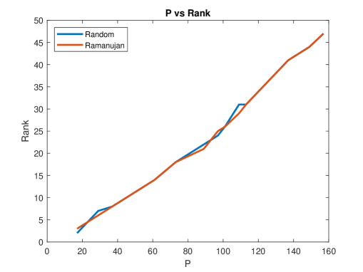
Figure 1: Critical value of rank versus the degree of the LPS Ramanujan graph with 1,092 vertices

$d$	$\bar{r}$	$\bar{r}/d$
198	62	0.3147
230	75	0.3275
294	102	0.3481

Table 1: Degree vs. critical rank in high degree LPS Ramanujan graphs

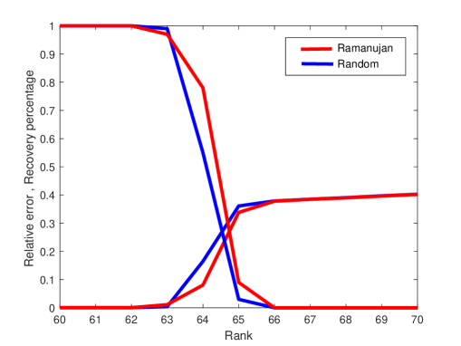
Figure 2: Phase transition behavior in LPS graph with 1,092 vertices with $p=197$

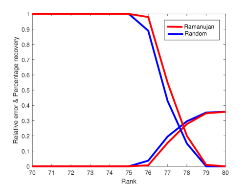
Figure 3: Phase transition behavior in LPS graph with 1,092 vertices with $p=229$

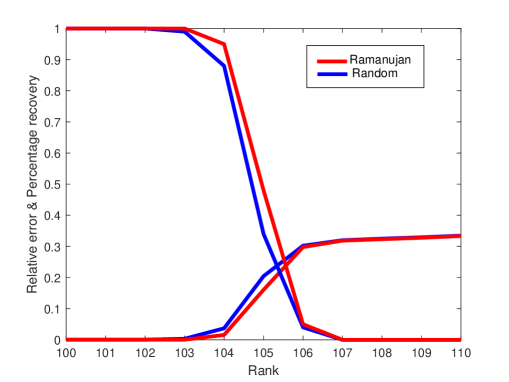
Figure 4: Phase transition behavior in LPS graph with 1,092 vertices with $p=293$

6.2 Comparison with Previous Studies

The phenomenon of phase transition is well-known in the case of vector recovery using $\ell_{1}$-norm minimization. It is also well-understood, and is discussed in several papers by David Donoho, such as [41, 42, 43, 44, 45, 46, 47, 48]. A very general theory of the behavior of convex optimization on randomly generated data is given in [49]. A concept called the “statistical dimension” is introduced, and it is established that convex optimization exhibits “phase transition,” whereby the success rate of the optimization algorithm goes from 100% to 0% very quickly as the input to the algorithm is changed. The width of the transition region is linear in the statistical dimension. In contrast, there are relatively fewer papers that have studied phase transition in matrix completion, and a proper theory is not yet available. In principle, the theory in [49] applies also to matrix completion using nuclear norm minimization. However, it is not easy to work out the appropriate statistical dimension in this case. In [22], the behaviour of the manifold approach to recovering randomly generated matrices is studied. A related paper is [50], which studies matrix recovery, and not matrix completion. In that paper, the measurements consist of taking the Frobenius inner product of the unknown matrix with randomly generated Gaussian matrices.

Now we describe some of the prior work on phase transition in matrix completion via nuclear norm minimization. In all the studies described below, the unknown matrix $X$ is assumed to be square, so we use the neutral symbol $n=n_{c}=n_{c}$ to denote its size. Throughout, $r$ denotes its rank, and $m$ denotes the number of measurements, that is, $|\Omega|$. This is consistent with the notation in the present paper, though the notation in the papers discussed below is in general different. Note that in some papers, $X$ satisfies additional constraints such as symmetry, positive semidefiniteness, Hankel or Toeplitz structure, etc. In [1], which first introduced this approach, there are some examples based on randomly generated low-rank matrices with $n=40$ or $n=50$. In [23], $n=500$, and $r\in\{10,20,40\}$. In [28], $n=11$ or $n=15$. In [29], $n=50$. In [31], $n=300$. Finally, in [27], $n=1,000$, and $r/n\in[0.04,0.4]$. In all cases, it is observed that the critical rank $r_{0}$ at which the recovery ratio drops sharply from 100% to 0% is essentially linear in $m$, the number of measurements. In our setting, since $m=dn$ where $d$ is the degree of the Ramanujan graph, this translates to $r_{0}$ being linear in $d$, as observed in the next subsection. Thus, to summarize, available numerical studies (including ours), indicate the presence of a phase transition, and a linear relationship between the critical rank $r_{0}$ and the number of measurements $m$.

7 Conclusions and Future Work

In this paper we have studied the matrix completion problem with emphasis on choosing the elements to be sampled in a deterministic fashion. We do this by choosing the sample matrix to equal the biadjacency matrix of an asymmetric Ramanujan graph, or Ramanujan bigraph. We have derived a sufficient condition that guarantees exact recovery of the unknown matrix with noise-free measurements using nuclear norm minimization, and stable recovery under non-sparse noisy measurements. We believe that we are presenting the very first correct result on exact recovery using nuclear norm minimization and a deterministic sampling pattern. An earlier paper [17, Theorem 4.2] claims a similar result, but there is one step in the proof that we believe is not justified. This is elaborated in the Appendix.

The sufficient condition given here is very conservative. It requires that the degree of the Ramanujan graph should be $\Omega(r^{3})$ where $r$ is the rank of the matrix to be recovered. Turning this around, our result implies that given a Ramanujan graph of degree $d$, we can guarantee exact recovery only when $r=O(d^{1/3})$. This naturally raises the question as to how close is the sufficient condition derived here to being necessary? Our numerical simulations have shown that $d\approx 3r$ seems to be sufficient to recover randomly generated matrices of rank $r$. More interesting, if $r$ is increased by just two or three above this critical value of $d/3$, the percentage of the randomly generated matrices that are recovered falls from 100% to 0%, a phenomenon known as “phase transition.”

One of the advantages of the random sampling approach is that it is relatively easy to account for “missing” measurements, by ensuring that the missing location is never sampled. In the present approach, this leads to a very interesting problem in graph theory, namely the construction of Ramanujan graphs when there is a “bar” on having edges between specified pairs of vertices. The authors are exploring this question, which would be of considerable interest to graph theorists, quite apart from the matrix completion researchers.

Appendix

In this appendix we point out an error in the proof of [17, Theorem 4.2], which is based on a recursion lemma [17, Lemma 7.3]. However, the proof of the recursion lemma is not given in [17], but is found in the longer version of the paper in [51]. On page 19 of [51], the third displayed (but unnumbered) equation is as follows:

$$\sum_{k=1}^{r}\|\hat{u}.U_{k}\|_{2}^{2} = \sum_{k=1}^{r}\sum_{l=1}^{n}\langle U_{\perp}^{i},U_{\perp}^{l}\rangle^{2}U_{lk}^{2}$$ (77)

$$= \sum_{l=1}^{n}\langle U_{\perp}^{i},U_{\perp}^{l}\rangle^{2}\|U^{l}\|_{2}^{2}$$

$$=^{(a)} \sum_{l=1}^{n}\langle U^{i},U^{l}\rangle^{2}\|U^{l}\|_{2}^{2}$$

$$\leq (\mu_{0}r/n)^{2},$$

where $\hat{u}=U_{\perp}U_{\perp}^{i}$.

Let us focus on the claimed equality highlighted by us as $(a)$. This equation is incorrect. If we represent $U_{\perp}U_{\perp}^{\top}$ as $(I_{n_{r}}-UU^{\top})$, then by orthogonality we have

$$\langle U^{i},U^{j}\rangle+\langle U_{\perp}^{i},U_{\perp}^{j}\rangle=0\;\forall i\neq j,$$

which in turn implies that

$$|\langle U^{i},U^{j}\rangle|=|\langle U_{\perp}^{i},U_{\perp}^{j}\rangle|\ \forall i\neq j.$$ (78)

However, when $i=j$, we have that

$$\|U^{i}\|_{2}^{2}+\|U_{\perp}^{i}\|_{2}^{2}=1\;\Longrightarrow\;\langle U_{\perp}^{i},U_{\perp}^{i}\rangle=1-\langle U^{i},U^{i}\rangle$$

for all $i$. Therefore

$$\|U_{\perp}^{i}\|_{2}^{2}=\|U^{i}\|_{2}^{2}\;\Longrightarrow\;\|U_{\perp}^{i}\|_{2}^{2}=\|U^{i}\|_{2}^{2}=1/2.$$

More elaborately

$$\sum_{l=1}^{n}\langle U_{\perp}^{i},U_{\perp}^{l}\rangle^{2}\|U^{l}\|_{2}^{2} = \|U_{\perp}^{i}\|_{2}^{4}\|U^{i}\|_{2}^{2}$$

$$+ \sum_{l\neq i}\langle U_{\perp}^{i},U_{\perp}^{l}\rangle^{2}\|U^{l}\|_{2}^{2}$$

$$= (1-\|U^{i}\|_{2}^{2})^{2}\|U^{i}\|_{2}^{2}$$

$$+ \sum_{l\neq i}\langle U^{i},U^{l}\rangle^{2}\|U^{l}\|_{2}^{2}$$

$$= \sum_{l=1}^{n}\langle U^{i},U^{l}\rangle^{2}\|U^{l}\|_{2}^{2}$$

$$+ (1-2\|U^{i}\|_{2}^{2})\|U^{i}\|_{2}^{2}.$$

Therefore, unless $\|U^{i}\|_{2}^{2}=1/2$ or zero, the step highlighted as $(a)$ in (77) is false for that value of $i$. The conclusion is that, in order for (77) to hold, every row of $U$ must either be identically zero, or have Euclidean norm of $1/2$. A row of $U$ being identically zero makes the corresponding row of the unknown matrix $X$ also identically zero. In short, (78) cannot hold except under extremely restrictive and unrealistic conditions. Similar reasoning is used for $V$ which is also not correct. Hence using this Lemma 7.3 in bounding $\|{\cal P}_{{\cal T}^{\perp}}(Y)\|_{S}$ on page 12 of [51] makes the proof of the Theorem 4.2 incorrect. However, it is of course possible that the theorem itself is correct.

References

- [1] E. Candès and B. Recht, “Exact matrix completion via convex optimization,” Foundations of of Computational Mathematics, vol. 9, pp. 717–772, 2008.
- [2] C. Tomasi and T. Kanade, “Shape and motion from image streams under orthography: A factorization method,” International Journal of Computer Vision, vol. 9, no. 2, pp. 137–154, 1992.
- [3] A. Shabani, R. L. Kosut, M. Mohseni, H. Rabitz, M. A. Broome, M. P. Almeida, A. Fedrizzi, and A. G. White, “Efficient measurement of quantum dynamics via compressive sensing,” Physical Review Letters, vol. 106, p. 100401, March 2011.
- [4] A. V. Rodionov, A. Veitia, R. Barends, J. Kelly, D. Sank, J. Wenner, J. M. Martinis, R. L. Kosut, and A. N. Korotkov, “Compressed sensing quantum process tomography for superconducting quantum gates,” Physical Review B, vol. 90, p. 144504, October 2014.
- [5] A. Kalev, R. L. Kosut, and I. H. Deutsch, “Quantum tomography protocols with positivity are compressed sensing protocols,” Quantum Information, vol. 1, p. 15018, 2015.
- [6] D. Gross, Y.-K. Liu, S. Flammi, S. Becker, and J. Eisert, “Quantum state tomography via compressed sensing,” Physical Review Letters, vol. 105, no. 15, pp. 150 401–150 404, October 2010.
- [7] Y.-K. Liu, “Universal low-rank matrix recovery from pauli measurements,” in Advances in Neural Information Processing Systems, 2011, pp. 1638–1646.
- [8] S. T. Flammia, D. Gross, Y.-K. Liu, and J. Eisert, “Quantum tomography via compressed sensing: Error bounds, sample complexity, and efficient estimators,” arxiv, p. 1205.2300, 2012.
- [9] D. Xia, “Estimation of low rank density matrices by pauli measurements,” Electronic Journal of Statistics, vol. 11, pp. 50–77, 2017.
- [10] M. A. Davenport and J. Romberg, “An overview of low-rank matrix recovery from incomplete observations,” IEEE J. of Selected Topics in Signal Processing, vol. 10, no. 4, pp. 608–622, June 2016.
- [11] B. Recht, M. Fazel, and P. Parrilo, “Guaranteed minimum rank solutions to linear matrix equations via nuclear norm minimization,” SIAM Review, vol. 52(3), pp. 471–501, 2010.
- [12] M. Fazel, H. Hindi, and S. P. Boyd, “A rank minimization heuristic with application to minimum order system approximation,” in Proceedings of the American Control Conference, 2001, pp. 4734–4739.
- [13] E. J. Candès and Y. Plan, “Matrix completion with noise,” Proceedings of the IEEE, vol. 98, no. 6, pp. 925–936, June 2010.
- [14] Y. Chen, “Incoherence-optimal matrix completion,” IEEE Transactions on Information Theory, vol. 61, no. 5, pp. 2909–2923, 2015.
- [15] B. Recht, “A simpler approach to matrix completion,” Journal of Machine Learning Research, vol. 12, pp. 3413–3430, 2011.
- [16] E. Heiman, G. Schechtman, and A. Shraibman, “Deterministic algorithms for matrix completion,” Random Structures and Algorithms, pp. 1–13, 2013.
- [17] S. Bhojanapalli and P. Jain, “Universal matrix completion,” in Proceedings of The 31st International Conference on Machine Learning, 2014, pp. 1881–1889.
- [18] M. Ashraphijuo and X. Wang, “Fundamental conditions for low-cp-rank tensor completion,” Journal of Machine Learning Research, vol. 18, no. 63, pp. 1–29, 2017.
- [19] F. Király, L. Theran, and R. Tomioka, “The algebraic combinatorial approach for low-rank matrix completion,” Machine Learning, vol. 16, pp. 1391–1436, 2015.
- [20] M. Ashraphijuo, V. Aggarwal, and X. Wang, “On deterministic sampling patterns for robust low-rank matrix completion,” IEEE Signal Processing Letters, vol. 25, no. 3, pp. 343–347, 2018.
- [21] S. P. Burnwal and M. Vidyasagar, “Deterministic completion of rectangular matrices using ramanujan bigraphs – i: Error bounds and exact recovery using asymmetric Ramanujan graphs,” arXiv:1908.00963v2, pp. 1–24, 2019.
- [22] D. Pimentel-Alarcón, N. Boston, and R. D. Nowak, “A characterization of deterministic sampling patterns for low-rank matrix completion,” IEEE Journal of Selected Topics in Signal Processing, vol. 10, no. 4, pp. 623–636, 2016.
- [23] R. H. Keshavan, A. Montanari, and S. Oh, “Matrix completion from a few entries,” IEEE Transactions on Information Theory, vol. 56, p. 2980–2998, 2010.
- [24] ——, “Matrix completion from noisy entries,” Journal of Machine Learning Research, vol. 11, pp. 2057–2078, 2010.
- [25] S. Burer and R. D. C. Monteiro, “A nonlinear programming algorithm for solving semidefinite programs via low-rank factorization,” Mathematical Programming (Series B), vol. 95, pp. 329–357, 2003.
- [26] Z. Zhu, Q. Li, G. Tang, and M. B. Wakin, “Global optimality in low-rank matrix optimization,” IEEE Transactions on Signal Processing, vol. 66, no. 13, pp. 3614–3628, July 2018.
- [27] Y. Yang, Y. Feng, and J. A. K. Suykens, “Correntropy based matrix completion,” Entropy, vol. 20, no. 171, pp. 1–23, 2018.
- [28] Y. Chen and Y. Chi, “Robust spectral compressed sensing via structured matrix completion,” IEEE Transactions on Information Theory, vol. 60, no. 10, pp. 6576–6601, October 2014.
- [29] Y. Chen, Y. Chi, and A. Goldsmith, “Exact and stable covariance estimation from quadratic sampling via convex programming,” IEEE Transactions on Information Theory, vol. 61, no. 7, pp. 4034–4059, July 2015.
- [30] T. T. Cai and A. Zhang, “ROP: Matrix recovery via rank-one projections,” Annals of Statistics, vol. 43, no. 1, pp. 102–138, 2015.
- [31] S. Zhang, Y. Hao, M. Wang, and J. H. Chow, “Multichannel hankel matrix completion through nonconvex optimization,” IEEE Journal of Selected Topics in Signal Processing, vol. 12, no. 4, pp. 617–632, August 2018.
- [32] M. R. Murty, “Ramanjuan graphs,” Journal of the Ramanujan Mathematical Society, vol. 18, no. 1, pp. 1–20, 2003.
- [33] G. Davidoff, P. Sarnak, and A. Valette, Elementary Number Theory, Group Theory, and Ramanujan Graphs. Cambridge University Press, 2003.
- [34] A. Nilli, “On the second eigenvalue of a graph,” Discrete Mathematics, vol. 91, no. 2, pp. 207–210, 1991.
- [35] S. Hoory, N. Linial, and A. Widgerson, “Expander graphs and their application,” Bulletin of the American Mathematical Society (New Series), vol. 43, no. 4, pp. 439–561, October 2006.
- [36] K. Feng and W.-C. W. Li, “Spectra of hypergraphs and applications,” Journal of number theory, vol. 60, no. 1, pp. 1–22, 1996.
- [37] S. P. Burnwal, M. Vidyasagar, and K. Sinha, “Deterministic completion of rectangular matrices using Ramanujan bigraphs – ii: Explicit constructions and phase transitions,” arXiv:1910.03937v1, pp. 1–25, 2019.
- [38] A. Marcus, D. A. Spielman, and N. Srivastava, “Interlacing families iv: Bipartite Ramanujan graphs of all sizes,” in 2015 IEEE 54th Annual Symposium on Foundations of Computer Science, 2015, pp. 1358–1367.
- [39] M. B. Cohen, “Ramanujan graphs in polynomial time,” arXiv:1604.03544v1.
- [40] A. Lubotzky, R. Phillips, and P. Sarnak, “Ramanujan graphs,” Combinatorica, vol. 8, no. 3, pp. 261–277, 1988.
- [41] D. L. Donoho and J. Tanner, “Neighborliness of randomly projected simplices in high dimensions,” Proceedings of the National Academy of Sciences, vol. 102, pp. 9452–9457, July 2005.
- [42] D. L. Donoho, A. Maleki, and A. Montanari, “Message-passing algorithms for compressed sensing,” Proceedings of the National Academy of Sciences, vol. 106, no. 45, pp. 18 914–18 919, 2009.
- [43] D. L. Donoho and J. Tanner, “Counting faces of randomly projected polytopes when the projection radically lowers dimension,” Journal of the American Mathematical Society, vol. 22, no. 1, pp. 1–53, January 2009.
- [44] D. Donoho and J. Tanner, “Observed universality of phase transitions in high-dimensional geometry, with implications for modern data analysis and signal processing,” Philosophical Transactions of The Royal Society, Part A: Mathematical, Physical and Engineering Sciences, vol. 367, no. 1906, pp. 4273–4293, November 2009.
- [45] D. L. Donoho and J. Tanner, “Precise undersampling theorems,” Proceedings of the IEEE, vol. 98, no. 6, pp. 913–924, June 2010.
- [46] D. L. Donoho, A. Javanmard, and A. Montanari, “Information-theoretically optimal compressed sensing via spatial coupling and approximate message passing,” in Proceedings of the International Symposium on Information Theory, 2012, pp. 1231–1235.
- [47] D. L. Donoho, I. Johnstone, and A. Montanari, “Accurate prediction of phase transitions in compressed sensing via a connection to minimax denoising,” IEEE Transactions on Information Theory, vol. 59, no. 6, pp. 3396–3433, June 2013.
- [48] D. L. Donoho, A. Javanmard, and A. Montanari, “Information-theoretically optimal compressed sensing via spatial coupling and approximate message passing,” IEEE Transactions on Information Theory, vol. 59, no. 11, pp. 7434–7464, November 2013.
- [49] D. Amelunxen, M. Lotz, M. B. McCoy, and J. A. Tropp, “Living on the edge: Phase transitions in convex programs with random data,” Information and Inference, vol. 3, no. 3, pp. 224–294, 2014.
- [50] D. L. Donoho, M. Gavish, and A. Montanari, “The phase transition of matrix recovery from Gaussian measurements matches the minimax MSE of matrix denoising,” Proceedings of the National Academy of Sciences, vol. 110, no. 21, pp. 8405–8410, 2013.
- [51] S. Bhojanapalli and P. Jain, “Universal matrix completion,” arxiv:1402.2324v2, pp. 1–22, July 2014.