Random sequential adsorption of k-mers on the fully-connected lattice: probability distributions of the covering time and extreme value statistics

Abstract

We study the random sequential adsorption of $k$-mers on the fully-connected lattice with $N=kn$ sites. The probability distribution $T_{n}(s,t)$ of the time $t$ needed to cover the lattice with $s$ $k$-mers is obtained using a generating function approach. In the low coverage scaling limit where $s,n,t\to\infty$ with $y=s/n^{1/2}=\mathrm{O}(1)$ the random variable $t-s$ follows a Poisson distribution with mean $ky^{2}/2$. In the intermediate coverage scaling limit, when both $s$ and $n-s$ are $\mathrm{O}(n)$, the mean value and the variance of the covering time are growing as $n$ and the fluctuations are Gaussian. When full coverage is approached the scaling functions diverge, which is the signal of a new scaling behaviour. Indeed, when $u=n-s=\mathrm{O}(1)$, the mean value of the covering time grows as $n^{k}$ and the variance as $n^{2k}$, thus $t$ is strongly fluctuating and no longer self-averaging. In this scaling regime the fluctuations are governed, for each value of $k$, by a different extreme value distribution, indexed by $u$. Explicit results are obtained for monomers (generalized Gumbel distribution) and dimers.

• Keywords: k-mers, fully-connected lattice, extreme value statistics

1 Introduction

Random sequential adsorption (RSA) is one of the simplest model of irreversible process in which particles of various shapes are deposited randomly on a substrate, one at a time (see [1, 2, 3, 4] for reviews). The process takes place either on a lattice or in the continuum. Overlap is forbidden and once deposited a particle remains fixed forever. It follows that, on a finite system, after some time there is not enough place left on the surface to add a new particle: a jammed configuration is reached.

The RSA model is expected to describe the adsorption of proteins, colloids or macromolecules on homogeneous substrates for which the relaxation time is much longer than the deposition time [5, 6]. The model have also been used in the study of crystal growth, glass formation and reactions on polymer chains [2].

Quantities of interest are the jamming fraction, which depends on the initial conditions, and the kinetics governing the approach to the jammed state.

Exact results have been mostly obtained in one dimension (1d) [7, 8, 9, 10, 11, 12, 13, 14, 15, 16, 17, 18]. For dimer deposition on a lattice, the jamming density is $x_{jam}=1-\rme^{-2}=0.864664\ldots$, a result first obtained by Flory in a study of the cyclization reaction along a polymer chain [7]. This limit is approached exponentially in time [15].

When unit length particles are deposited at arbitrary random positions along a line (continuous RSA), one obtains the car parking problem solved by Rényi [8, 10]. The jamming density has a complicated mathematical expression such that $x_{jam}=0.747597\ldots$ and the approach to saturation is algebraic, namely, $x_{jam}-x(t)\sim t^{-1}$ [8, 10, 4].

Analytical results are sparse in higher dimensions and restricted to limited domains of time evolution and density. Numerical studies suggest that, like in 1d, the approach to jamming is generally exponential in time for deposition on a lattice while it is algebraic on a continuous substrate [1, 2, 3, 4]. In the latter case, the jamming exponent is $1/d$ for isotropic objects [6, 19, 20] while it departs from this value for unoriented anisotropic objects [21, 22, 23, 24, 25, 26, 27].

An exception to this lack of exact results is provided by the deposition of dimers on the Cayley tree with coordination number $z$, a problem which can be solved using the empty connected cluster method [28]. The jamming density, $x_{jam}=1-(z-1)^{-z/(z-2)}$ , is approached exponentially in time [28, 4].

In the present work we study the RSA of $k$-mers on the fully connected lattice, a problem for which the time evolution of the density $x(t)$ has been obtained in 1d [4]. Here the emphasis is put on the probability distribution of the covering time, its scaling behaviours at low and intermediate coverage and its extreme value statistics in the vicinity of full coverage. This is a continuation of previous works about random walks and reaction-diffusion processes on the complete graph [29, 30, 31, 32].

Note that for monomers our results remain valid for any homogeneous lattice with $N=n$ sites in any dimension. Furthermore, the RSA of monomers on the fully-connected lattice is equivalent to the covering of the lattice by a random walk [29, 30] as well as to the coupon collector’s problem [33, 34, 35, 36, 37].

The outline of the paper is as follows. In section 2 the model is described, solved in the mean-field approximation and the main results are presented. Section 3 deals with the probability distribution $T_{n}(s,t)$ of the time $t$ needed to covers a finite-size lattice with $s$ $k$-mers. An ordinary generating function is written down, leading to a general expression for $T_{n}(s,t)$ which is afterwards specified for $k$-mers. The same is done for the moments of the distribution. In section 4 , using a master equation approach, the behaviour of the covering time is studied in three different scaling regimes: first at low coverage when $s=\mathrm{O}(n^{1/2})$, then at intermediate coverage when both $s$ and $n-s=\mathrm{O}(n)$ and finally in the extreme value limit, when $n-s=\mathrm{O}(1)$. We conclude in section 5 and give some complements on the calculations in five appendices.

2 Model, mean field and main results

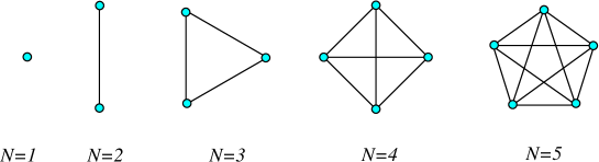
Figure 1: The fully-connected lattice (complete graph) with $N$ sites can be embedded in a Euclidean space of dimension $d=N-1$. The addition of a new site equidistant from the previous ones requires a new dimension. Therefore all sites belong to the surface.

2.1 Model

We study the RSA of $k$-mers on a fully-connected lattice with $N=kn$ equivalent sites. For such a lattice, by construction, all the sites belong to the surface and can be occupied by $k$-mers (see figure 1). Moreover, whatever the value of $k$, the lattice can always be fully covered.

At each time step $k$ distinct sites are selected at random among the $N$. Multiple occupancy being forbidden, a new $k$-mer can be adsorbed only when the $k$ selected sites are empty. If $s$ $k$-mers are already covering the lattice, $k(n-s)$ sites among the $kn$ remain free and the attempt will be successful with probability

$$p_{n}(s)=\frac{{k(n-s)\choose k}}{{kn\choose k}}=\frac{[k(n-s)]^{\underline{k}}}{(kn)^{\underline{k}}}\,,$$ (2.1)

where $j^{\underline{k}}$ is the falling factorial power $j(j-1)\ldots(j-k+1)$ [38] and $n$ is the maximum number of adsorbed $k$-mers, corresponding to full coverage.

2.2 Mean-field theory

Let $x=s/n$ be the surface coverage, i.e., the fraction of lattice sites covered by $k$-mers and $w=t/n$ a rescaled time variable. In the intermediate coverage scaling limit (icsl) where $s,t,n\to\infty$ with $0<x<1$ and $w=\mathrm{O}(1)$ the transition probability in (2.1) takes the following form:

$$p(x)\stackrel{{\scriptstyle\rm icsl}}{{=}}(1-x)^{k}\,.$$ (2.2)

In the mean-field approximation, during the time interval $dt$ the number of $k$-mers adsorbed on the lattice changes by $ds=ndx=p(x)dt=p(x)ndw$. It follows that:

$$\frac{dw}{dx}=\frac{1}{(1-x)^{k}}\,.$$ (2.3)

With the initial condition $w\to 0$ when $x\to 0$ one obtains:

$$\frac{t}{n}\stackrel{{\scriptstyle\rm icsl}}{{=}}w=\frac{1}{k-1}\left[\frac{1}{(1-x)^{k-1}}-1\right]\,,\qquad k>1\,.$$ (2.4)

The limit $k\to 1$ gives the following logarithmic behaviour:

$$w=-\ln(1-x)\,,\qquad k=1\,.$$ (2.5)

Extracting the $k$-mer density from these expressions leads to:

$$x=\left\{\begin{array}[]{ccc}1-[1+(k-1)w]^{-1/(k-1)}\,,&k>1\,,\\ \,1-e^{-w}\,,&k=1\,.\end{array}\right.$$ (2.6)

2.3 Main results

The finite-size probability distribution $T_{n}(s,t)$ of the time $t$ needed to cover the lattice with $s$ $k$-mers has been obtained as a function of the transition probability $p_{n}(s)$ for any value of $k$ (see (3.6)).

Depending on the fraction of occupied sites $x=s/n$ three different scaling regimes are observed when $n$, $s$ and $t$ tend to infinity:

• In the low coverage scaling limit (lcsl), when $y\stackrel{{\scriptstyle\rm lcsl}}{{=}}s/n^{1/2}=\mathrm{O}(1)$ so that $x\stackrel{{\scriptstyle\rm lcsl}}{{=}}0$, the probability distribution $D_{n}(s,v)=T_{n}(s,t=s+v)$ converges to the Poisson distribution with mean $\overline{v}=ky^{2}/2$

  $${\mathfrak{P}}_{v}(y)=\frac{(ky^{2}/2)^{v}}{v!}\exp\left(-\frac{ky^{2}}{2}\right)\,,\qquad{\mathfrak{P}}_{v}(0)=\delta_{v,0}\,,$$ (2.7)

  which is the solution of the difference-differential equation

  $$\frac{\partial{\mathfrak{P}}_{v}}{\partial y}=ky\left[{\mathfrak{P}}_{v-1}(y)-{\mathfrak{P}}_{v}(y)\right]\,,$$ (2.8)

  following from the master-equation governing $D_{n}(s,v)$ in this scaling limit.

• In the intermediate coverage scaling limit (icsl), when both $s$ and $n-s$ are $\mathrm{O}(n)$ so that $0<x<1$, the mean covering time $\overline{t_{n}}$ and the variance $\overline{\Delta t_{n}^{2}}$ are growing as $n$ and $n^{1/2}T_{n}(s,t)$ converges to the Gaussian probability density

  $${\mathfrak{T}}(x,\tau)=\frac{\exp\left[-\frac{\tau^{2}}{2g(x)}\right]}{\sqrt{2\pi g(x)}}\,,\qquad\tau\stackrel{{\scriptstyle\rm icsl}}{{=}}\frac{t-\overline{t_{n}}}{n^{1/2}}\,,$$ (2.9)

  where $\overline{t_{n}}$ is the mean-field result in (2.4) and (2.5). The variance is given by:

  $$\frac{\overline{\Delta t_{n}^{2}}}{n}\stackrel{{\scriptstyle\rm icsl}}{{=}}g(x)=\left\{\begin{array}[]{ccc}\frac{1}{2k-1}\left[\frac{1}{(1-x)^{2k-1}}-1\right]-\frac{1}{k-1}\left[\frac{1}{(1-x)^{k-1}}-1\right]\,,&k>1\,,\\ \,\frac{x}{1-x}+\ln(1-x)\,,&k=1\,.\end{array}\right.$$ (2.10)

  Both $\overline{t_{n}}$ and $\overline{\Delta t_{n}^{2}}$ vanish when $x\to 0$ and diverge when $x\to 1$. These divergences indicate a new scaling behaviour at $x=1$

• In the extreme value scaling limit (evsl) when $u=n-s=\mathrm{O}(1)$ so that $x\stackrel{{\scriptstyle\rm evsl}}{{=}}1$, $\overline{t_{n}}$ is growing as $(kn)^{\underline{k}}$ and $\overline{\Delta t_{n}^{2}}$ as $[(kn)^{\underline{k}}]^{2}$. Thus the system is non-self-averaging. The appropriate scaling variable is now $\tau^{\prime}=t/(kn)^{\underline{k}}-\delta_{k,1}\ln n$. In the scaling limit, the master equation governing the behaviour of $T_{n}(s,t)$ leads to the following difference-differential equation

  $$\frac{\partial{\mathfrak{T}}^{\prime}_{u}}{\partial\tau^{\prime}}=[k(u+1)]^{\underline{k}}\left[{\mathfrak{T}}^{\prime}_{u+1}(\tau^{\prime})-{\mathfrak{T}}^{\prime}_{u}(\tau^{\prime})\right]$$ (2.11)

  for the extreme value distribution ${\mathfrak{T}}^{\prime}_{u}(\tau^{\prime})\stackrel{{\scriptstyle\rm evsl}}{{=}}(kn)^{\underline{k}}\,T_{n}(s,t)$. The solution for monomers is the generalized Gumbel distribution [33, 39]:

  $${\mathfrak{T}}^{\prime}_{u}(\tau^{\prime})=\frac{1}{u!}\exp[-(u+1)\tau^{\prime}-\rme^{-\tau^{\prime}}]\,.$$ (2.12)

  Taking directly the scaling limit on the scaled probability distribution, the following expression is obtained for dimers:

  $${\mathfrak{T}}^{\prime}_{u}(\tau^{\prime})=\frac{1}{(2u)!}\sum_{j=0}^{\infty}(-1)^{j}\frac{(4u+4j+3)(4u+2j+1)!!}{(2j)!!}\,\rme^{-(2u+2j+1)(2u+2j+2)\tau^{\prime}}\,.$$ (2.13)

  For each value of $k$ there is a different extreme value distribution of the scaled time, indexed by $u$.

3 Finite-size results

In this section we study the probability distribution $T_{n}(s,t)$ of the time $t$ needed to adsorb irreversibly $s$ $k$-mers on the fully-connected lattice with $kn$ sites. $T_{n}(s,t)$ and its moments are obtained using generating functions techniques for general values of $p_{n}(s)$ before specifying the form of the transition probability for $k$-mers.

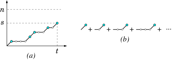
Figure 2: A time evolution of the number of $k$-mers covering the lattice is sketched in (a). A big circle corresponds to the successful deposition (probability $p_{n}(\beta)$) of a $k$-mer on the lattice covered by $\beta$ $k$-mers, a small circle to a failed attempt. The diagrams in (b) give the contributions to the generating function of the probability distribution $L_{n}(\beta,t)$ of the waiting time $t$ in a state with $\beta$ $k$-mers defined in (3.2).

3.1 Generating function for $T_{n}(s,t)$

The probability distribution of the covering time $T_{n}(s,t)$ will be deduced from the generating function:

$${\mathcal{T}}_{n}(s,z)=\sum_{t=1}^{\infty}z^{t}T_{n}(s,t)\,.$$ (3.1)

Let $\beta$ be the intermediate number of $k$-mers deposited on the lattice, its evolution from 0 to $s$ in figure 2(a) takes place through sequences where the system remains for some time in a state with a constant value of $\beta$, ending with a transition, $\beta\to\beta+1$. To the probability distribution of the waiting time, $L_{n}(\beta,l)$ one can associate the generating function ${\mathcal{L}}_{n}(\beta,z)$ corresponding to the diagrams of figure 2(b):

$${\mathcal{L}}_{n}(\beta,z) =\!\sum_{l=1}^{\infty}z^{l}L_{n}(\beta,l)\!=\!\{1\!+\!z[1\!-p_{n}(\beta)]\!+\!z^{2}[1\!-p_{n}(\beta)]^{2}\!+\cdots\}zp_{n}(\beta)$$ (3.2)

$$=\frac{zp_{n}(\beta)}{1-z[1-p_{n}(\beta)]}\,.$$

The generating function we are looking for is simply obtained as the product

$${\mathcal{T}}_{n}(s,z)=\prod_{\beta=0}^{s-1}{\mathcal{L}}_{n}(\beta,z)=z^{s}\prod_{\beta=0}^{s-1}\frac{p_{n}(\beta)}{1-z[1-p_{n}(\beta)]}\,.$$ (3.3)

Note that ${\mathcal{T}}_{n}(s,1)=\sum_{t=1}^{\infty}T_{n}(s,t)=1$ as required.

3.2 General expression of $T_{n}(s,t)$

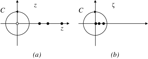
Figure 3: Integration contour $C$ used to extract $T_{n}(s,t)$ from its generating function in (3.4). (a) In the z-plane $C$ is the unit circle, centered at the origin and oriented counter-clockwise. The integrand has a pole at the origin when $t\geq s$ and $s$ simple poles outside $C$ on the positive real axis. (b) Through the transformation $\zeta=1/z$, the unit circle transforms into itself, but $C$ is now oriented clockwise. The pole at the origin is sent to infinity and the $s$ simple poles are transported inside $C$.

According to (3.1) the probability distribution, which is the coefficient of $z^{t}$ in the series expansion of ${\mathcal{T}}_{n}(s,z)$ in (3.3), is given by the following contour integral:

$$T_{n}(s,t) =\frac{1}{2i\pi}\oint_{\stackrel{{\scriptstyle\curvearrowleft}}{{C}}}dz\frac{{\mathcal{T}}_{n}(s,z)}{z^{t+1}}=\frac{1}{2i\pi}\oint_{\stackrel{{\scriptstyle\curvearrowleft}}{{C}}}\frac{dz}{z^{t-s+1}}\prod_{\beta=0}^{s-1}\frac{p_{n}(\beta)}{1-z[1-p_{n}(\beta)]}$$ (3.4)

$$=\frac{1}{2i\pi}\oint_{\stackrel{{\scriptstyle\curvearrowleft}}{{C}}}\frac{dz}{z^{t+1}}\prod_{\beta=0}^{s-1}\frac{p_{n}(\beta)}{1/z-[1-p_{n}(\beta)]}\,.$$

The contour $\stackrel{{\scriptstyle\curvearrowleft}}{{C}}$ is a unit circle, oriented counter-clockwise and centered at the origin. Besides the pole at the origin for $t\geq s$, the integrand has $s$ simple poles $z_{\alpha}=[1-p_{n}(\alpha)]^{-1}$ on the positive real axis outsides $\stackrel{{\scriptstyle\curvearrowleft}}{{C}}$ since $0<p_{n}(\alpha)\leq 1$ by assumption.

As shown in figure 3, the change of variable $\zeta=1/z$ transforms the contour $\stackrel{{\scriptstyle\curvearrowleft}}{{C}}$ into $\stackrel{{\scriptstyle\curvearrowright}}{{C}}$, a unit circle with a clockwise orientation. It sends to infinity the pole at the origin and introduces $s$ simple poles $\zeta_{\alpha}=[1-p_{n}(\alpha)]<1$ inside $\stackrel{{\scriptstyle\curvearrowright}}{{C}}$ so that:

$$T_{n}(s,t)=-\frac{1}{2i\pi}\oint_{\stackrel{{\scriptstyle\curvearrowright}}{{C}}}d\zeta\,\zeta^{t-1}\prod_{\beta=0}^{s-1}\frac{p_{n}(\beta)}{\zeta\!-\![1\!-\!p_{n}(\beta)]}=\frac{1}{2i\pi}\oint_{\stackrel{{\scriptstyle\curvearrowleft}}{{C}}}d\zeta\,\zeta^{t-1}\prod_{\beta=0}^{s-1}\frac{p_{n}(\beta)}{\zeta\!-\![1\!-\!p_{n}(\beta)]}\,.$$ (3.5)

Finally, applying the theorem of residues, one obtains the probability distribution

$$T_{n}(s,t)=\prod_{\beta=0}^{s-1}p_{n}(\beta)\sum_{\alpha=0}^{s-1}\frac{[1-p_{n}(\alpha)]^{t-1}}{\prod_{\beta=0\atop\beta\neq\alpha}^{s-1}[p_{n}(\beta)-p_{n}(\alpha)]}\,.$$ (3.6)

3.3 Explicit expression of $T_{n}(s,t)$ for $k$-mers

It will be convenient to express $T_{n}(s,t)$ as a function of $u=n-s$ in order to study the scaling limit when $u=\mathrm{O}(1)$. According to (2.1) the probability distribution in (3.6) can be rewritten as:

$$T_{n}(s,t)=\sum_{\alpha=0}^{s-1}\frac{ab}{cd}\,p_{n}(\alpha)[1-p_{n}(\alpha)]^{t-1}\,,\quad a=\prod_{\beta=0}^{\alpha-1}[k(n-\beta)]^{\underline{k}}\,,\quad b=\prod_{\beta=\alpha+1}^{s-1}[k(n-\beta)]^{\underline{k}}\,,$$

$$c=\prod_{\beta=0}^{\alpha-1}\left\{[k(n-\beta)]^{\underline{k}}-[k(n-\alpha)]^{\underline{k}}\right\}\,,\quad d=\prod_{\beta=\alpha+1}^{s-1}\left\{[k(n-\beta)]^{\underline{k}}-[k(n-\alpha)]^{\underline{k}}\right\}\,.$$ (3.7)

With the change of variables

$$\alpha=s-j-1=n-u-j-1\,,\qquad\beta=s-i-1=n-u-i-1\,,$$ (3.8)

one obtains

$$c\!=\!\!\!\prod_{i=j+1}^{n-u-1}\!\!\left\{[k(u\!+\!i\!+\!1)]^{\underline{k}}\!-\![k(u\!+\!j\!+\!1)]^{\underline{k}}\right\}\,,\quad d\!=\!(-1)^{j}\prod_{i=0}^{j-1}\left\{[k(u\!+\!j\!+\!1)]^{\underline{k}}\!-\![k(u\!+\!i\!+\!1)]^{\underline{k}}\right\}\,,$$

$$a=\frac{(kn)!}{[k(u\!+\!j+\!1)]!}\,,\quad b=\frac{[k(u\!+\!j)]!}{(ku)!}\,,\quad ab\,p_{n}(\alpha)=\frac{(kn)!}{(kn)^{\underline{k}}(ku)!}\,,$$ (3.9)

so that:

$$T_{n}(n-u,t)=\frac{(kn)!}{(kn)^{\underline{k}}(ku)!}\sum_{j=0}^{n-u-1}\frac{1}{cd}\left\{1-\frac{[k(u\!+\!j+\!1)]^{\underline{k}}}{(kn)^{\underline{k}}}\right\}^{t-1}\,.$$ (3.10)

When $k=1$, the probability distribution has a simple expression [30] in terms of Stirling’s numbers of the second kind [40]:

$$T_{n}(s,t)=\frac{n^{\underline{s}}}{n^{t}}{t-1\brace s-1}\,,\qquad{t\brace s}=\frac{1}{s!}\sum_{j=0}^{s}(-1)^{s-j}{s\choose j}j^{t}\,.$$ (3.11)

3.4 Moments of the probability distribution

Since the covering time $t(s)$ is the sum from $\beta=0$ to $s-1$ of the waiting times, $l(\beta)$, which are independent random variables, its mean value and variance are given by the corresponding sums for the waiting times.

3.4.1 Mean value.

The mean value of the waiting time in a state with $\beta$ adsorbed $k$-mers is given by the first derivative at $z=1$ of the generating function ${\mathcal{L}}_{n}(\beta,z)$ in (3.2)

$$\overline{l_{n}(\beta)}=\sum_{l=1}^{\infty}l\,L_{n}(\beta,l)=\left.\frac{\partial{\mathcal{L}}_{n}}{\partial z}\right|_{z=1}=\frac{1}{p_{n}(\beta)}\,,$$ (3.12)

so that:

$$\overline{t_{n}(s)}=\sum_{\beta=0}^{s-1}\frac{1}{p_{n}(\beta)}\,.$$ (3.13)

3.4.2 Variance.

A second derivative gives the mean square value

$$\overline{l_{n}^{2}(\beta)}=\sum_{l=1}^{\infty}l^{2}L_{n}(\beta,l)=\left.\frac{\partial}{\partial z}\left[z\frac{\partial{\mathcal{L}}_{n}}{\partial z}\right]\right|_{z=1}=\frac{2-p_{n}(\beta)}{p_{n}^{2}(\beta)}\,,$$ (3.14)

from which follows the variance:

$$\overline{\Delta l_{n}^{2}(\beta)}=\overline{l_{n}^{2}(\beta)}-\overline{l_{n}(\beta)}^{2}=\frac{1-p_{n}(\beta)}{p_{n}^{2}(\beta)}=\frac{1}{p_{n}^{2}(\beta)}-\overline{l_{n}(\beta)}\,.$$ (3.15)

Thus the variance of the covering time is given by:

$$\overline{\Delta t_{n}^{2}(s)}=\sum_{\beta=0}^{s-1}\frac{1}{p_{n}^{2}(\beta)}-\overline{t_{n}(s)}\,.$$ (3.16)

3.5 Explicit expressions of the moments for k-mers

3.5.1 Mean value.

The mean value of the covering time, following from (3.13) and (2.1), is given by:

$$\overline{t_{n}(s)}=\sum_{\beta=0}^{s-1}\frac{(kn)^{\underline{k}}}{[k(n-\beta)]^{\underline{k}}}=\sum_{j=n-s+1}^{n}\frac{(kn)^{\underline{k}}}{(kj)^{\underline{k}}}\,.$$ (3.17)

Using (1.1) in appendix A, one obtains:

$$\overline{t_{n}(s)}=\frac{(kn)^{\underline{k}}}{(k-1)!}\sum_{j=n-s+1}^{n}\sum_{l=0}^{k-1}(-1)^{k-l-1}\frac{{k-1\choose l}}{kj-l}\,.$$ (3.18)

As shown in appendix B, this expression can be rewritten using harmonic and generalized harmonic numbers, under a form which is appropriate to obtain the scaling limit when $u=n-s=\mathrm{O}(1)$:

$$\ \ \overline{t_{n}} =\frac{(kn)^{\underline{k}}}{(k-1)!}\left[H_{kn}-H_{ku}+(\delta_{k,1}-1)(H_{n}-H_{u})+\sum_{m=2}^{\infty}\frac{H_{n}^{(m)}-H_{u}^{(m)}}{k^{m}}\;P_{k,m}\right]\,,$$

$$P_{k,m} =\sum_{l=0}^{k-1}\left[(-1)^{k-l-1}{k-1\choose l}-1\right]l^{m-1}\,.$$ (3.19)

For monomers and dimers this expression reduces to:

$$k =1\,,\quad\overline{t_{n}} =n\,(H_{n}-H_{u})\,,$$

$$k =2\,,\quad\overline{t_{n}} =(2n)^{\underline{2}}\,(H_{2n}-H_{2u}-H_{n}+H_{u})\,.$$ (3.20)

3.5.2 Variance.

Using (2.1) and (1.1) the first contribution to the variance in (3.16) is given by:

$$\sum_{\beta=0}^{s-1}\frac{1}{p_{n}^{2}(\beta)}=\overline{\Delta t_{n}^{2}(s)}+\overline{t_{n}(s)}=\left[\frac{(kn)^{\underline{k}}}{(k-1)!}\right]^{2}\sum_{j=n-s+1}^{n}\sum_{l,l^{\prime}=0}^{k-1}(-1)^{l+l^{\prime}}\frac{{k-1\choose l}{k-1\choose l^{\prime}}}{(kj-l)(kj-l^{\prime})}\,.$$ (3.21)

As above for the mean value, this expression can be rewritten in terms of generalized harmonic numbers (see appendix C):

$$\overline{\Delta t_{n}^{2}}\!+\overline{t_{n}} =\left[\frac{(kn)^{\underline{k}}}{(k-1)!}\right]^{2}\left\{H_{kn}^{(2)}\!-\!H_{ku}^{(2)}\!+\!\sum_{m=2}^{\infty}\frac{H_{n}^{(m)}\!-\!H_{u}^{(m)}}{k^{m}}\left[(m\!-\!1)Q_{k,m}\!+\!2R_{k,m}\right]\right\}\,,$$

$$\quad\ Q_{k,m} =\sum_{l=0}^{k-1}\left[{k-1\choose l}^{2}-1\right]l^{m-2}\,,$$

$$\quad\ R_{k,m} =\sum_{l>l^{\prime}=0}^{k-1}(-1)^{l+l^{\prime}}{k-1\choose l}{k-1\choose l^{\prime}}\frac{l^{m-1}-{l^{\prime}}^{m-1}}{l-l^{\prime}}\,.$$ (3.22)

Thus for monomers and dimers, taking (3.20) into account, the variance is given by:

$$k=1\,,\quad\overline{\Delta t_{n}^{2}}=n^{2}[H_{n}^{(2)}-H_{u}^{(2)}]-n(H_{n}-H_{u})\,,$$

$$k=2\,,\quad\overline{\Delta t_{n}^{2}}=[(2n)^{\underline{2}}]^{2}[H_{2n}^{(2)}-H_{2u}^{(2)}]-(2n)^{\underline{2}}[2(2n)^{\underline{2}}+1](H_{2n}-H_{2u}-H_{n}+H_{u})\,.$$ (3.23)

4 Scaling limits

In this section we study the different scaling limits of the problem using a master-equation approach .

4.1 Master equations

Let $S_{n}(s,t)$ be the probability to have $s$ k-mers covering $ks$ sites on the lattice at time $t$ and $p_{n}(s)$ the probability to add a k-mer on the lattice with $s$ k-mers. Between $t$ and $t+1$, $s\rightarrow s$ with probability $1-p_{n}(s)$ and $s-1\rightarrow s$ with probability $p_{n}(s-1)$ thus $S_{n}(s,t)$ evolves according to the following master equation:

$$S_{n}(s,t+1)=[1-p_{n}(s)]S_{n}(s,t)+p_{n}(s-1)S_{n}(s-1,t).$$ (4.1)

The probability distribution of the time $t$ needed to adsorb $s$ $k$-mers (first-passage time by the value $s$) is given by:

$$T_{n}(s,t)=S_{n}(s-1,t-1)p_{n}(s-1)\,.$$ (4.2)

According to (4.1), its time evolution is governed by the following master equation:

$$T_{n}(s,t+1)=[1-p_{n}(s-1)]T_{n}(s,t)+p_{n}(s-1)T_{n}(s-1,t).$$ (4.3)

Changing $t$ into $t-1$ in (4.3) the probability distribution $D_{n}(s,v)=T_{n}(s,t)$ with $v=t-s$ evolves as follows:

$$D_{n}(s,v)=[1-p_{n}(s-1)]D_{n}(s,v-1)+p_{n}(s-1)D_{n}(s-1,v).$$ (4.4)

4.2 Low coverage scaling limit

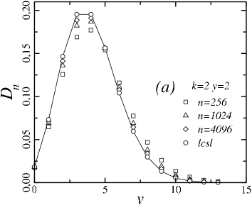
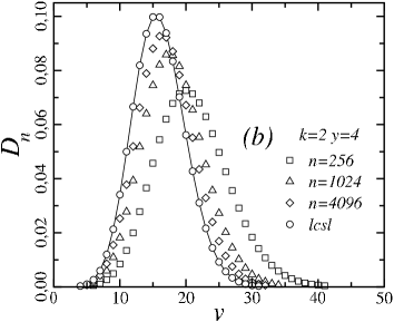
Figure 4: (a) Finite-size data collapse on the Poisson distribution ${\mathfrak{P}}_{v}(y)\stackrel{{\scriptstyle\rm lcsl}}{{=}}D_{n}(s,v)$ in (4.14) versus $v=t-s$ when $k=2$ and $y=s/n^{1/2}=2$. (b) When $y=4$, for the same sizes, the convergence to the limit distribution is much slower. The system crosses over from Poisson to Gauss when $n$ decreases ($x=y/n^{1/2}$).

In the lcsl, first considered in [33] for the coupon collector’s problem, $s,t,n\to\infty$ with $s=\mathrm{O}(n^{1/2})$ so that:

$$y\stackrel{{\scriptstyle\rm lcsl}}{{=}}\frac{s}{n^{1/2}}=\mathrm{O}(1)\,,\qquad x=\frac{s}{n}=\frac{y}{n^{1/2}}\stackrel{{\scriptstyle\rm lcsl}}{{=}}0\,.$$ (4.5)

Let us look for the form of the master equation (4.4) in this scaling limit where we define:

$${\mathfrak{P}}_{v}(y)={\mathfrak{P}}_{v}[y(s)]\stackrel{{\scriptstyle\rm lcsl}}{{=}}D_{n}(s,v)\,,\qquad v\in\mathbb{N}_{0}\,.$$ (4.6)

Since $y(s-1)=y-n^{-1/2}$, a first order expansion gives:

$${\mathfrak{P}}_{v}[y(s-1)]={\mathfrak{P}}_{v}(y)-\frac{1}{n^{1/2}}\frac{\partial{\mathfrak{P}}_{v}}{\partial y}+\mathrm{O}(n^{-1})\,.$$ (4.7)

According to (2.1), one has:

$$p_{n}(s-1)=\prod_{j=0}^{k-1}\left[\frac{k(n-s+1)-j}{kn-j}\right]=\left(1-\frac{y}{n^{1/2}}\right)^{k}+\mathrm{O}(n^{-1})=1-\frac{ky}{n^{1/2}}+\mathrm{O}(n^{-1})\,.$$ (4.8)

Thus the master equation (4.4) can be rewritten as:

$${\mathfrak{P}}_{v}(y)=\frac{ky}{n^{1/2}}{\mathfrak{P}}_{v-1}(y)+\left(1-\frac{ky}{n^{1/2}}\right)\left[{\mathfrak{P}}_{v}(y)-\frac{1}{n^{1/2}}\frac{\partial{\mathfrak{P}}_{v}}{\partial y}\right]+\mathrm{O}(n^{-1})\,.$$ (4.9)

The leading contribution, of order $n^{-1/2}$, gives the following difference-differential equation for ${\mathfrak{P}}_{v}(y)$:

$$\frac{\partial{\mathfrak{P}}_{v}}{\partial y}=ky\left[{\mathfrak{P}}_{v-1}(y)-{\mathfrak{P}}_{v}(y)\right]\,.$$ (4.10)

Making use of the generating function

$${\mathcal{D}}(\lambda,y)=\sum_{v=0}^{\infty}\lambda^{v}{\mathfrak{P}}_{v}(y)\,,$$ (4.11)

equation (4.10) transforms into:

$$\frac{\partial{\mathcal{D}}}{\partial y}=ky(\lambda-1){\mathcal{D}}(\lambda,y)\,.$$ (4.12)

The solution satisfying ${\mathcal{D}}(1,y)=1$ reads

$${\mathcal{D}}(\lambda,y)=\exp\left[(\lambda-1)\frac{ky^{2}}{2}\right]\,,$$ (4.13)

which is the generating function of the Poisson distribution given by

$${\mathfrak{P}}_{v}(y)=\frac{(ky^{2}/2)^{v}}{v!}\exp\left(-\frac{ky^{2}}{2}\right)\,,$$ (4.14)

in agreement with [33] when $k=1$. The convergence of the finite-size data, obtained by iterating 4.4, to the Poisson distribution is shown in figure 4. Since $s$ is non-fluctuating, one obtains:

$$\overline{v}=ky^{2}/2\stackrel{{\scriptstyle\rm lcsl}}{{=}}\overline{t_{n}}-s\,,\qquad\overline{\Delta v^{2}}=ky^{2}/2\stackrel{{\scriptstyle\rm lcsl}}{{=}}\overline{\Delta t_{n}^{2}}\,.$$ (4.15)

These results can be verified using (2.1) in (3.13) and (3.16), in the same limit. When $y=0$, i.e., when $s=\mathrm{O}(n^{\alpha})$ with $\alpha<1/2$, ${\mathfrak{P}}_{v}(0)=\delta_{v.0}$.

4.3 Intermediate coverage scaling limit

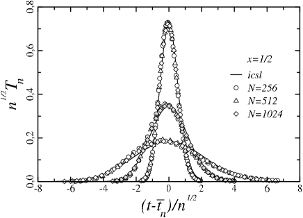
Figure 5: Finite-size data collapse on the Gaussian density ${\mathfrak{T}}\stackrel{{\scriptstyle\rm icsl}}{{=}}n^{1/2}T_{n}$ in (4.23) versus $\tau=(t-\overline{t_{n}})/n^{1/2}$ for $k=1,2,3$ from top to bottom. The fraction of occupied sites is $x=s/n=1/2$. The finite-size results were obtained by iterating (4.3).

In this section we look for the behaviour of $T_{n}(s,t)$ in the intermediate coverage scaling limit (icsl), where both $s$ and $u=n-s$ are $\mathrm{O}(n)$, so that $0<x<1$ when $n\to\infty$.

The mean-field results (2.4) and (2.5) suggest that $\overline{t_{n}}$ is scaling as $n$ and a similar behaviour is expected for the variance so that we write:

$$\frac{\overline{t_{n}}}{n}\stackrel{{\scriptstyle\rm icsl}}{{=}}f(x)\,,\qquad\frac{\overline{\Delta t_{n}^{2}}}{n}\stackrel{{\scriptstyle\rm icsl}}{{=}}g(x)\,.$$ (4.16)

The appropriate time variable may then be defined as (see figure 5)

$$\tau(s,t)\stackrel{{\scriptstyle\rm icsl}}{{=}}\frac{t-\overline{t_{n}}}{n^{1/2}}=\frac{t}{n^{1/2}}-n^{1/2}f\left(\frac{s}{n}\right)\,,$$ (4.17)

with the associated probability density given by:

$${\mathfrak{T}}(x,\tau)={\mathfrak{T}}[x(s),\tau(s,t)]\stackrel{{\scriptstyle\rm icsl}}{{=}}n^{1/2}T_{n}(s,t)\,.$$ (4.18)

Proceeding as above (see appendix D), at order $n^{-1/2}$ the expansion of the master equation (4.3) gives a differential equation (4.2) for $f(x)$ such that, with the initial condition $f(0)=0$

$$f(x)\stackrel{{\scriptstyle\rm icsl}}{{=}}\frac{\overline{t_{n}}}{n}=\left\{\begin{array}[]{ccc}\frac{1}{k-1}\left[\frac{1}{(1-x)^{k-1}}-1\right]\,,&k>1\\ \,-\ln(1-x)\,,&k=1\end{array}\right.\,,$$ (4.19)

in agreement with the mean-field results (2.4) and (2.5). This scaling function is shown in figure 6(a). When $x\to 0$, $f(x)\sim x$, i.e., each deposition attempt is successful, as expected. When $x\to 1$, $f(x)$ diverges logarithmically for $k=1$ and as $(1-x)^{-(k-1)}$ for $k>1$.

The terms of order $n^{-1}$ provide the partial differential equation (4.3) for ${\mathfrak{T}}(x,\tau)$.

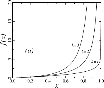
Figure 6: Scaling functions (a) $f(x)\stackrel{{\scriptstyle\rm icsl}}{{=}}\overline{t_{n}}/n$ and (b) $g(x)\stackrel{{\scriptstyle\rm icsl}}{{=}}\overline{\Delta t_{n}^{2}}/n$ versus $x=s/n$ for $k=1,2,3$. The two functions diverge when $x\to 1$, which is the signal of a different scaling behaviour in this limit. Note the change of the vertical scale.

Assuming that ${\mathfrak{T}}(x,\tau)$ depends on $x$ through $g$, the scaling function of the variance, i.e.

$${\mathfrak{T}}(x,\tau)={\mathfrak{Q}}[g(x),\tau]\,,$$ (4.20)

the partial differential equation can be rewritten as:

$$\frac{\partial{\mathfrak{Q}}}{\partial g}\frac{dg}{dx}=\frac{1}{2}\underbrace{\left[\frac{1}{(1-x)^{2k}}-\frac{1}{(1-x)^{k}}\right]}_{dg/dx}\frac{\partial^{2}{\mathfrak{Q}}}{\partial\tau^{2}}\,.$$ (4.21)

The standard diffusion equation is obtained when

$$\frac{dg}{dx}=\left[\frac{1}{(1-x)^{2k}}-\frac{1}{(1-x)^{k}}\right]\,,$$ (4.22)

so that:

$${\mathfrak{T}}(x,\tau)={\mathfrak{Q}}[g(x),\tau]=\frac{\exp\left[-\frac{\tau^{2}}{2g(x)}\right]}{\sqrt{2\pi g(x)}}\,.$$ (4.23)

The solution of (4.22) is immediate and given by

$$g(x)\stackrel{{\scriptstyle\rm icsl}}{{=}}\frac{\overline{\Delta t_{n}^{2}}}{n}=\left\{\begin{array}[]{ccc}\frac{1}{2k-1}\left[\frac{1}{(1-x)^{2k-1}}-1\right]-\frac{1}{k-1}\left[\frac{1}{(1-x)^{k-1}}-1\right]\,,&k>1\\ \,\frac{x}{1-x}+\ln(1-x)\,,&k=1\end{array}\right.\,.$$ (4.24)

for $g(0)=0$. The behaviour of this scaling function is shown in figure 6(b). For any value of $k$, $g(x)$ vanishes as $kx^{2}/2$ when $x\to 0$ and diverges as $(1-x)^{-(2k-1)}$ when $x\to 1$.

The cross-over from Poisson to Gauss at low density is discussed in appendix E. The divergence of $f(x)$ and $g(x)$ when $x\to 1$ indicates a different scaling behaviour when $u=n-s=\mathrm{O}(1)$. This extreme value limit is studied in the next section.

4.4 Extreme value scaling limit

Let us finally study the approach to saturation when $s,t,n\to\infty$ with $u=n-s=\mathrm{O}(1)$ so that $x=1-u/n\stackrel{{\scriptstyle\rm evsl}}{{=}}1$. In this extreme-value regime, strong fluctuations of the covering time and anomalous scaling behaviour are expected.

4.4.1 Mean value.

In the limit where $n\to\infty$, according to (3.19), one obtains

$$\frac{\overline{t_{n}}}{(kn)^{\underline{k}}}-\delta_{k,1}\ln n\!\stackrel{{\scriptstyle\rm evsl}}{{=}}\!\frac{1}{(k\!-\!1)!}\left[\ln k\!+\!\delta_{k,1}\gamma\!-\!H_{ku}\!+\!(1\!-\!\delta_{k,1})\!H_{u}\!+\!\sum_{m\!=\!2}^{\infty}\!\frac{\zeta(m)\!-\!H_{u}^{(m)}}{k^{m}}P_{k,m}\right]\!,$$ (4.25)

where $\gamma=0.577\,215\,665\,\ldots$ is the Euler-Mascheroni constant, $\zeta(m)$ is the Riemann zeta function and $P_{k,m}$ is defined in (3.19). For monomers and dimers (3.20) leads to:

$$k =1\,,\quad\frac{\overline{t_{n}}}{n}-\ln n\stackrel{{\scriptstyle\rm evsl}}{{=}}\gamma-H_{u}\,,$$

$$k =2\,,\quad\frac{\overline{t_{n}}}{(2n)^{\underline{2}}}\stackrel{{\scriptstyle\rm evsl}}{{=}}\ln 2-H_{2u}+H_{u}\,.$$ (4.26)

4.4.2 Variance.

For the variance (3.22) gives

$$\frac{\overline{\Delta t_{n}^{2}}}{\left[(kn)^{\underline{k}}\right]^{2}} \!\stackrel{{\scriptstyle\rm evsl}}{{=}}\frac{1}{[(k-1)!]^{2}}\left\{\zeta(2)\!-\!H_{ku}^{(2)}\!+\!\sum_{m=2}^{\infty}\frac{\zeta(m)\!-\!H_{u}^{(m)}}{k^{m}}\left[(m\!-\!1)Q_{k,m}\!+\!2R_{k,m}\right]\right\}\,,$$ (4.27)

with $Q_{k,m}$ and $R_{k,m}$ as defined in (3.22). For monomers and dimers (3.23) leads to:

$$k =1\,,\quad\frac{\overline{\Delta t_{n}^{2}}}{n^{2}}\stackrel{{\scriptstyle\rm evsl}}{{=}}\zeta(2)-H_{u}^{(2)}\,,$$

$$k =2\,,\quad\frac{\overline{\Delta t_{n}^{2}}}{[(2n)^{\underline{2}}]^{2}}\stackrel{{\scriptstyle\rm evsl}}{{=}}\zeta(2)-H_{2u}^{(2)}-2(\ln 2-H_{2u}+H_{u})\,.$$ (4.28)

4.4.3 Master equation in the extreme value scaling limit.

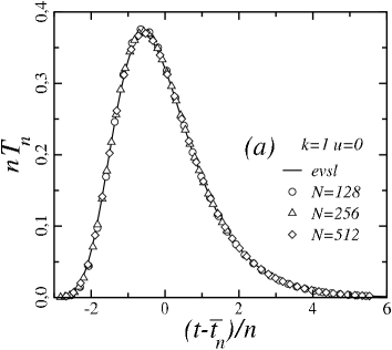
Figure 7: Finite-size data collapse on (a) the Gumble distribution ${\mathfrak{T}}^{\prime}_{0}(\tau^{\prime})\stackrel{{\scriptstyle\rm evsl}}{{=}}nT_{n}(n,t)$ in (4.50) versus $\tau^{\prime}-\overline{\tau^{\prime}}=(t-\overline{t_{n}})/n$ when $k=1$ and $u=0$, (b) the probability density ${\mathfrak{T}}^{\prime}_{0}(\tau^{\prime})\stackrel{{\scriptstyle\rm evsl}}{{=}}(2n)^{\underline{2}}T_{n}(n,t)$ in (4.57) versus $\tau^{\prime}-\overline{\tau^{\prime}}=(t-\overline{t_{n}})/(2n)^{\underline{2}}$ when $k=2$ and $u=0$. The finite-size data were obtained by iterating (4.3).

According to (4.25) and (4.27), $\overline{t_{n}}$ and $\sqrt{\overline{\Delta t_{n}^{2}}}$ are both growing as $(kn)^{\underline{k}}$ when $u=\mathrm{O}(1)$. Thus, in the scaling limit, we define a new time variable

$$\tau^{\prime}=\frac{t}{(kn)^{\underline{k}}}-\delta_{k,1}\ln n$$ (4.29)

to which corresponds the probability density (see figure 7)

$${\mathfrak{T}}^{\prime}_{u}(\tau^{\prime})\stackrel{{\scriptstyle\rm evsl}}{{=}}(kn)^{\underline{k}}T_{n}(s,t)\,,\qquad u=n-s=\mathrm{O}(1)\,.$$ (4.30)

In the master equation (4.3), the transition probability is given by:

$$p_{n}(s-1)=\frac{[k(n-s+1)]^{\underline{k}}}{(kn)^{\underline{k}}}\stackrel{{\scriptstyle\rm evsl}}{{=}}\frac{[k(u+1)]^{\underline{k}}}{(kn)^{k}}\,.$$ (4.31)

A first-order Taylor expansion of ${\mathfrak{T}}^{\prime}_{u}\left[\tau^{\prime}+(kn)^{-k}\right]$ on the left-hand-side of the master equation (4.3) leads to:

$${\mathfrak{T}}^{\prime}_{u}(\tau^{\prime})\!+\!\frac{1}{(kn)^{k}}\frac{\partial{\mathfrak{T}}^{\prime}_{u}(\tau^{\prime})}{\partial\tau^{\prime}}\!=\!\left\{\!1\!-\frac{[k(u\!+\!1)]^{\underline{k}}}{(kn)^{k}}\right\}{\mathfrak{T}}^{\prime}_{u}(\tau^{\prime})\!+\!\frac{[k(u\!+\!1)]^{\underline{k}}}{(kn)^{k}}{\mathfrak{T}}^{\prime}_{u+1}(\tau^{\prime})\!+\!\mathrm{O}(n^{-2k})\,.$$ (4.32)

$\mathrm{O}(1)$ terms disappear leaving $\mathrm{O}(n^{-k})$ terms from which the following difference-differential equation is deduced:

$$\frac{\partial{\mathfrak{T}}^{\prime}_{u}(\tau^{\prime})}{\partial\tau^{\prime}}=[k(u+1)]^{\underline{k}}\left[{\mathfrak{T}}^{\prime}_{u+1}(\tau^{\prime})-{\mathfrak{T}}^{\prime}_{u}(\tau^{\prime})\right]\,.\$$ (4.33)

Introducing the generating function

$${\mathfrak{T}}^{\prime}(\mu,\tau^{\prime})=\sum_{u=0}^{\infty}\mu^{ku}{\mathfrak{T}}^{\prime}_{u}(\tau^{\prime})\,,$$ (4.34)

one has:

$$\sum_{u=0}^{\infty}[k(u+1)]^{\underline{k}}\mu^{ku}{\mathfrak{T}}^{\prime}_{u+1}(\tau^{\prime})=\frac{\partial^{k}}{\partial\mu^{k}}\sum_{u=0}^{\infty}\mu^{k(u+1)}{\mathfrak{T}}^{\prime}_{u+1}(\tau^{\prime})$$

$$\ \ \ \ \ \ \ \ \ \ \ \ \ \ \ \ \ =\frac{\partial^{k}}{\partial\mu^{k}}\left[\sum_{u^{\prime}=0}^{\infty}\mu^{ku^{\prime}}{\mathfrak{T}}^{\prime}_{u^{\prime}}(\tau^{\prime})-{\mathfrak{T}}^{\prime}_{0}(\tau^{\prime})\right]=\frac{\partial^{k}}{\partial\mu^{k}}{\mathfrak{T}}^{\prime}(\mu,\tau^{\prime})$$

$$\sum_{u=0}^{\infty}[k(u+1)]^{\underline{k}}\mu^{ku}{\mathfrak{T}}^{\prime}_{u}(\tau^{\prime})\!=\!\frac{\partial^{k}}{\partial\mu^{k}}\sum_{u=0}^{\infty}\mu^{k(u+1)}{\mathfrak{T}}^{\prime}_{u}(\tau^{\prime})\!=\!\frac{\partial^{k}}{\partial\mu^{k}}\left[\mu^{k}{\mathfrak{T}}^{\prime}(\mu,\tau^{\prime})\right].$$ (4.35)

Thus the difference-differential equation (4.33) can be rewritten as a partial-differential equation for the generating function (4.34):

$$\frac{\partial{\mathfrak{T}}^{\prime}(\mu,\tau^{\prime})}{\partial\tau^{\prime}}=\frac{\partial^{k}}{\partial\mu^{k}}\left[(1-\mu^{k}){\mathfrak{T}}^{\prime}(\mu,\tau^{\prime})\right]\,.$$ (4.36)

4.4.4 ${\mathfrak{T}}^{\prime}(\mu,\tau^{\prime})$ for monomers.

Although it is possible to obtain the probability density through a direct evaluation of (3.10) in the scaling limit [30], here we shall instead deduce it from its generating function, ${\mathfrak{T}}^{\prime}(\mu,\tau^{\prime})$, solution of (4.36).

For monomers, according to (4.29) the scaled time is given by:

$$\tau^{\prime}\stackrel{{\scriptstyle\rm evsl}}{{=}}\frac{t}{n}-\ln n\,\qquad-\infty<\tau^{\prime}<+\infty\,.$$ (4.37)

Then according to (4.26)

$$\overline{\tau^{\prime}}=\gamma-H_{u}=-\Psi(u+1)\,,$$ (4.38)

where $\Psi(u)$ is the digamma function [41].

When $k=1$, the partial differential equation (4.36) reads:

$$\frac{1}{{\mathfrak{T}}^{\prime}}\frac{\partial{\mathfrak{T}}^{\prime}}{\partial\tau^{\prime}}=(1-\mu)\frac{1}{{\mathfrak{T}}^{\prime}}\frac{\partial{\mathfrak{T}}^{\prime}}{\partial\mu}-1\,.$$ (4.39)

The change of function ${\mathfrak{U}}^{\prime}=\ln{\mathfrak{T}}^{\prime}$ gives:

$$\frac{\partial{\mathfrak{U}}^{\prime}}{\partial\tau^{\prime}}=(1-\mu)\frac{\partial{\mathfrak{U}}^{\prime}}{\partial\mu}-1\,.$$ (4.40)

With

$${\mathfrak{U}}^{\prime}(\mu,\tau^{\prime})=-\tau^{\prime}+q(\tau^{\prime})r(\mu)\,,$$ (4.41)

the inhomogeneity is removed and, dividing by $qr$, the variables separate

$$\frac{1}{q}\frac{dq}{d\tau^{\prime}}=(1-\mu)\frac{1}{r}\frac{dr}{d\mu}=-c_{1}\,,$$ (4.42)

where $c_{1}$ is a constant. Thus one has

$$q(\tau^{\prime})=c_{2}\rme^{-c_{1}\tau^{\prime}}\,,\quad r(\mu)=c_{3}(1-\mu)^{c_{1}}\,,\quad{\mathfrak{U}}^{\prime}(\mu,\tau^{\prime})=-\tau^{\prime}-c^{\prime}_{2}(1-\mu)^{c_{1}}\rme^{-c_{1}\tau^{\prime}}\,,$$ (4.43)

where $c^{\prime}_{2}=-c_{2}c_{3}$ is a new constant and

$${\mathfrak{T}}^{\prime}(\mu,\tau^{\prime})=\sum_{u=0}^{\infty}\mu^{u}\,{\mathfrak{T}}^{\prime}_{u}(\tau^{\prime})=\exp\left[-\tau^{\prime}-c^{\prime}_{2}(1-\mu)^{c_{1}}\rme^{-c_{1}\tau^{\prime}}\right]\,.$$ (4.44)

$\mu=0$ selects the term $u=0$ in the sum over $u$ so that:

$${\mathfrak{T}}^{\prime}(0,\tau^{\prime})={\mathfrak{T}}^{\prime}_{0}(\tau^{\prime})=\exp\left[-\tau^{\prime}-c^{\prime}_{2}\rme^{-c_{1}\tau^{\prime}}\right]\,.$$ (4.45)

The integration constants can be determined using

$$\int_{-\infty}^{\infty}\!{\mathfrak{T}}^{\prime}(0,\tau^{\prime})d\tau^{\prime}\!=\!\int_{-\infty}^{\infty}\!{\mathfrak{T}}^{\prime}_{0}(\tau^{\prime})d\tau^{\prime}\!=\!1\,,\quad\int_{-\infty}^{\infty}\!\!\!\tau^{\prime}{\mathfrak{T}}^{\prime}(0,\tau^{\prime})d\tau^{\prime}\!=\!\int_{-\infty}^{\infty}\!\!\tau^{\prime}{\mathfrak{T}}^{\prime}_{0}(\tau^{\prime})d\tau^{\prime}\!=\!\overline{\tau^{\prime}}\!=\!\gamma\,,$$ (4.46)

the last relation following from (4.38) when $u=0$. With the change of variable $\theta=\rme^{-\tau^{\prime}}$, one obtains:

$$\int_{-\infty}^{\infty}\!\!{\mathfrak{T}}^{\prime}(0,\tau^{\prime})d\tau^{\prime}\!\!=\!\int_{0}^{\infty}\!\!\!\exp\left[-c^{\prime}_{2}\theta^{c_{1}}\right]d\theta\,,\quad\int_{-\infty}^{\infty}\!\!\!\tau^{\prime}{\mathfrak{T}}^{\prime}(0,\tau^{\prime})d\tau^{\prime}\!\!=\!-\!\int_{0}^{\infty}\!\!\ln\theta\exp\left[-c^{\prime}_{2}\theta^{c_{1}}\right]d\theta\,.$$ (4.47)

A new change of variable, $\rho=c^{\prime}_{2}\theta^{c_{1}}$, in the first integral leads to

$$\int_{-\infty}^{\infty}{\mathfrak{T}}^{\prime}(0,\tau^{\prime})d\tau^{\prime}=\frac{1}{{c^{\prime}_{2}}^{1/c_{1}}c_{1}}\int_{0}^{\infty}\rho^{1/c_{1}-1}\rme^{-\rho}d\rho=\frac{\Gamma(1/c_{1})}{c_{1}{c^{\prime}_{2}}^{1/c_{1}}}\,,\quad c^{\prime}_{2}=\left[\frac{\Gamma(1/c_{1})}{c_{1}}\right]^{c_{1}}\,,$$ (4.48)

where the last relation follows from the normalization of ${\mathfrak{T}}^{\prime}_{0}$ in (4.46). Inserting this value of $c^{\prime}_{2}$ in the second integral of (4.47) one obtains a standard integral representation of the Euler-Mascheroni constant [41] when $c_{1}=1$. Thus $c^{\prime}_{2}=c_{1}=1$ and (4.44) gives:

$${\mathfrak{T}}^{\prime}(\mu,\tau^{\prime})=\exp\left[-\tau^{\prime}-(1-\mu)\rme^{-\tau^{\prime}}\right]=\exp\left[-\tau^{\prime}-\rme^{-\tau^{\prime}}\right]\exp\left[\mu\,\rme^{-\tau^{\prime}}\right]\,.$$ (4.49)

The coefficient of $\mu^{u}$ in the power expansion of the last factor in (4.49) gives the sought probability density, which is a generalized Gumbel distribution [30, 42, 39]:

$${\mathfrak{T}}^{\prime}_{u}(\tau^{\prime})=\frac{1}{u!}\exp[-(u+1)\tau^{\prime}-\rme^{-\tau^{\prime}}]\,,\quad k=1\,,\quad-\infty<\tau^{\prime}<+\infty\,.$$ (4.50)

This result was previously obtained for the covering time by a random walk [30] by taking directly the extreme value scaling limit on $nT_{n}(s,t)$ with a centered scaling variable, $\tau^{\prime}-\overline{\tau^{\prime}}$. See also [33] where it was noticed that (4.50) is the $\chi^{2}$ distribution in the variable $2\rme^{-\tau^{\prime}}$ with $2(u+1)$ degrees of freedom.

The finite-size data collapse on the standard Gumbel distribution, corresponding to $u=0$, is shown in figure 7a.

4.4.5 ${\mathfrak{T}}^{\prime}_{u}(\tau^{\prime})$ for dimers.

\psfrag{X0}[Bc][Bc][1][1]{${\mathfrak{T}}^{\prime}_{0}$}\psfrag{x}[tc][tc][1][0]{$\tau^{\prime}-\overline{\tau^{\prime}}$}\includegraphics[width=184.9429pt,angle={0}]{fig-8a.eps}

\psfrag{X0}[Bc][Bc][1][1]{${\mathfrak{T}}^{\prime}_{0}$}\psfrag{x}[tc][tc][1][0]{$\tau^{\prime}-\overline{\tau^{\prime}}$}\psfrag{Xu}[Bc][Bc][1][1]{${\mathfrak{T}}^{\prime}_{u}$}\psfrag{x}[tc][tc][1][0]{$\tau^{\prime}-\overline{\tau^{\prime}}$}\includegraphics[width=184.9429pt,angle={0}]{fig-8b.eps}

Figure 8: Evolution of the probability density ${\mathfrak{T}}^{\prime}_{u}(\tau^{\prime})$ versus $\tau^{\prime}-\overline{\tau^{\prime}}$ for (a) $u=0$ and increasing values of $k$, (b) $k=2$ and increasing values of $u$.

For dimers, we take the scaling limit directly on the explicit expression (3.10) with $k=2$. According to (3.9),

$$c =\prod_{i=j+1}^{n-u-1}2(i-j)[2(i+j)+4u+3]=\frac{(2n-2u-2j-2)!!(2n+2u+2j+1)!!}{(4u+4j+3)!!}\,,$$

$$d =(-1)^{j}\prod_{i=0}^{j-1}2(j-i)[2(i+j)+4u+3]=(-1)^{j}\frac{(2j)!!(4u+4j+1)!!}{(4u+2j+1)!!}\,,$$ (4.51)

and (3.10) leads to:

$$(2n)^{\underline{2}}T_{n}(n-u,t)=\frac{(2n)!}{(2u)!}\sum_{j=0}^{n-u-1} \frac{(-1)^{j}(4u+4j+3)(4u+2j+1)!!}{(2j)!!(2n-2u-2j-2)!!(2n+2u+2j+1)!!}$$ (4.52)

$$\ \ \ \ \ \ \ \ \ \ \ \ \ \ \ \ \ \ \ \left\{1-\frac{[2(u\!+\!j+\!1)]^{\underline{2}}}{(2n)^{\underline{2}}}\right\}^{t-1}\,.$$

In the scaling limit with

$$\tau^{\prime}=t/(2n)^{\underline{2}}\,,\qquad 0\leq\tau^{\prime}<\infty\,,$$ (4.53)

such that, according to (4.26),

$$\overline{\tau^{\prime}}=\ln 2-H_{2u}+H_{u}\,,$$ (4.54)

one obtains:

$$\left\{1-\frac{[2(u\!+\!j+\!1)]^{\underline{2}}}{(2n)^{\underline{2}}}\right\}^{t-1}\stackrel{{\scriptstyle\rm evsl}}{{=}}\rme^{-(2u+2j+1)(2u+2j+2)\tau^{\prime}}\,.$$ (4.55)

Using $(2n)!=(2n)!!(2n-1)!!$ the $n$-dependent factors in (4.52) give

$$\frac{(2n)!!/(2n-2u-2j-2)!!}{(2n+2u+2j+1)!!/(2n-1)!!}=\frac{\overbrace{(2n)(2n-2)\ldots(2n-2u-2j)}^{u+j+1\ \mathrm{factors}}}{\underbrace{(2n+2u+2j+1)\ldots(2n+3)(2n+1)}_{u+j+1\ \mathrm{factors}}}\stackrel{{\scriptstyle\rm evsl}}{{=}}1$$ (4.56)

in the limit. Thus, for dimers, when $u=n-s=\mathrm{O}(1)$, the probability density of the covering time is given by:

$${\mathfrak{T}}^{\prime}_{u}(\tau^{\prime}) \stackrel{{\scriptstyle\rm evsl}}{{=}}(2n)^{\underline{2}}T_{n}(n-u,t)$$ (4.57)

$$=\frac{1}{(2u)!}\sum_{j=0}^{\infty}(-1)^{j}\frac{(4u+4j+3)(4u+2j+1)!!}{(2j)!!}\,\rme^{-(2u+2j+1)(2u+2j+2)\tau^{\prime}}\,.$$

The finite-size data collapse on this extreme value distribution is shown for $u=0$ in figure 7b.

4.4.6 ${\mathfrak{T}}^{\prime}_{u}(\tau^{\prime})$ for $k$-mers

Figure 8(a) shows the evolution with $k$ of ${\mathfrak{T}}^{\prime}_{0}$ as a function of $\tau^{\prime}-\overline{\tau^{\prime}}$. According to (3.10) and (4.29), for any value of $k$, the probability density decays exponentially at long time:

$${\mathfrak{T}}^{\prime}_{u}(\tau^{\prime})\sim\exp\left\{-[k(u+1)]^{\underline{k}}\,\tau^{\prime}\right\}\,,\qquad\tau^{\prime}\gg 1\,.$$ (4.58)

For increasing values of $u$ the probability density evolves from the asymmetric extreme value distribution towards a Gaussian. This is illustrated in figure 8(b) for dimers. Similar results can be found for $k=1$ in [30] where the cross-over is studied.

5 Conclusion

In this work we have studied the statistics of $k$-mers deposition on the fully-connected lattice. This lattice presents the peculiarity that, for any value of $k$, saturation occurs only at full coverage when the size $N$ is a multiple of $k$.

In the partial coverage regime, $0<x<1$, where mean-field theory is valid, the approach to full coverage is exponential in time for monomers and algebraic for $k>1$. Thus, for dimers, the approach to saturation is algebraic in time on the fully-connected lattice whereas it is exponential on the Cayley tree [28, 4].

The probability distribution $T_{n}(s,t)$ of the time $t$ needed to cover a finite-size system with $s$ $k$-mers, the mean value of the covering time and its variance have been obtained through a generating function approach.

Three different scaling regimes have been studied by taking the scaling limits on the master equations.

In the low coverage scaling limit ($x\stackrel{{\scriptstyle\rm lcsl}}{{=}}0$, $s/n^{1/2}\stackrel{{\scriptstyle\rm lcsl}}{{=}}y=\mathrm{O}(1))$, the probability distribution $D_{n}(s,v)=T_{n}(s,s+v)$ converges to a Poisson distribution in the variable $v=t-s$ with mean value and variance $ky^{2}/2$. Thus the random variable $t=s+v$ is self-averaging and a Kronecker delta distribution, $\delta_{v,0}$, is obtained when $y\stackrel{{\scriptstyle\rm lcsl}}{{=}}0$, i.e., when $s$ grows as $n^{\alpha}$ with $\alpha<1/2$.

In the intermediate coverage scaling limit ($0<x<1$, $s=\mathrm{O}(n)$, $n-s=\mathrm{O}(n)$), the covering time is self-averaging with Gaussian fluctuations. The mean value and the variance are growing as $n$. Their scaling functions are both diverging as $x\to 1$, signaling a new scaling behaviour in this limit. For the mean value the divergence is logarithmic when $k=1$ and algebraic when $k>1$, whereas it is always algebraic for the variance.

In the extreme value scaling limit ($x\stackrel{{\scriptstyle\rm evsl}}{{=}}1$, $u=n-s=\mathrm{O}(1)$) the mean value of the covering time grows as $n^{k}$ whereas its variance grows as $n^{2k}$, thus $t$ is no longer a self-averaging variable. The master equation then leads to a difference-differential equation, governing the extreme value distribution of the scaled covering time, for each value of $k$.

Using a generating function approach this equation has been solved for $k=1$. The fluctuations of the scaled covering time by monomers are governed by a generalized Gumbel distribution. Further work on the solution of the difference-differential equation is needed for $k>1$. For dimers, the scaling limit taken directly on $(2n)^{\underline{2}}T_{n}$ leads to an alternate infinite series. For any value of $k$ the extreme value distribution displays a $u$- and $k$-dependent exponential decay at long time and crosses over slowly to the Gaussian behaviour when $u$ increases.

Appendix A Inverse of a falling factorial power

Consider the relation:

$$A_{k}(a)=\frac{1}{a^{\underline{k}}}=\frac{1}{\prod_{l=0}^{k-1}(a-l)}=\frac{1}{(k-1)!}\sum_{l=0}^{k-1}(-1)^{k-l-1}\frac{{k-1\choose l}}{a-l}\,.$$ (1.1)

It is evidently true for $k=1$. Assuming it to be true for $k$, one has:

$$A_{k+1}(a)=\frac{A_{k}(a)}{a-k}=\frac{1}{(k-1)!}\sum_{l=0}^{k-1}(-1)^{k-l-1}\frac{{k-1\choose l}}{(a-l)(a-k)}\,.$$ (1.2)

Using

$$\frac{1}{(a-l)(a-k)}=\left(\frac{1}{a-k}-\frac{1}{a-l}\right)\frac{1}{k-l}\,,$$ (1.3)

(1.2) can be rewritten as:

$$A_{k+1}(a) =\frac{1}{a-k}\underbrace{\frac{1}{(k-1)!}\sum_{l=0}^{k-1}(-1)^{k-l-1}\frac{{k-1\choose l}}{k-l}}_{A_{k}(k)=1/k!}-\frac{1}{(k-1)!}\sum_{l=0}^{k-1}(-1)^{k-l-1}\frac{{k-1\choose l}}{(a-l)(k-l)}$$ (1.4)

$$=\frac{1}{k!(a-k)}+\frac{1}{k!}\sum_{l=0}^{k-1}(-1)^{k-l}\frac{{k\choose l}}{(a-l)}=\frac{1}{k!}\sum_{l=0}^{k}(-1)^{k-l}\frac{{k\choose l}}{(a-l)}\,.$$

Thus (1.1) is true for any value of $k$.

Appendix B From (3.18) to (3.19)

The sum over $l$ in (3.18) can be rewritten as:

$$\sum_{l=0}^{k-1}(-1)^{k-l-1}\frac{{k-1\choose l}}{kj-l}=\underbrace{\sum_{l=0}^{k-1}\frac{1}{kj-l}}_{B_{j}}+\underbrace{\sum_{l=0}^{k-1}\frac{(-1)^{k-l-1}{k-1\choose l}-1}{kj-l}}_{C_{j}}\,.$$ (2.1)

Summing the first term over $j$ gives

$$\sum_{j=u+1}^{n}B_{j}=H_{kn}-H_{ku}\,,$$ (2.2)

where $H_{j}=\sum_{i=1}^{j}1/i$ is a harmonic number. With

$$\frac{1}{kj-l}=\sum_{m=0}^{\infty}\frac{l^{m}}{(kj)^{m+1}}\,,$$ (2.3)

the last term contributes

$$\sum_{j=u+1}^{n}\!\!\!C_{j}=\sum_{m=0}^{\infty}\frac{H_{n}^{(m+1)}-H_{u}^{(m+1)}}{k^{m+1}}\sum_{l=0}^{k-1}\left[(-1)^{k-l-1}{k-1\choose l}-1\right]l^{m}\,,$$ (2.4)

where $H_{j}^{(m)}=\sum_{i=1}^{j}1/i^{m}$ is a generalized harmonic number. Since

$$\sum_{l=0}^{k-1}\left[(-1)^{k-l-1}{k-1\choose l}-1\right]=\delta_{k,1}-k\,,$$ (2.5)

one may separate the contribution from $m=0$ in (2.4) so that:

$$\sum_{j=u+1}^{n}\!\!\!C_{j}=(\delta_{k,1}-1)(H_{n}-H_{u})+\sum_{m=2}^{\infty}\frac{H_{n}^{(m)}\!-\!H_{u}^{(m)}}{k^{m}}\sum_{l=0}^{k-1}\left[(-1)^{k-l-1}{k\!-\!1\choose l}\!-\!1\right]l^{m-1}\!\!.$$ (2.6)

Making use of (2.2) and (2.6) in (3.18) finally gives (3.19).

Appendix C From (3.21) to (3.22)

The double sum in (3.21) may be splitted as:

$$\sum_{l,l^{\prime}=0}^{k-1}(-1)^{l+l^{\prime}}\frac{{k-1\choose l}{k-1\choose l^{\prime}}}{(kj-l)(kj-l^{\prime})} =\underbrace{\sum_{l=0}^{k-1}\frac{1}{(kj-l)^{2}}}_{D_{j}}+\underbrace{\sum_{l=0}^{k-1}\frac{{k-1\choose l}^{2}-1}{(kj-l)^{2}}}_{E_{j}}$$ (3.1)

$$+2\underbrace{\sum_{l>l^{\prime}=0}^{k-1}(-1)^{l+l^{\prime}}\frac{{k-1\choose l}{k-1\choose l^{\prime}}}{(kj-l)(kj-l^{\prime})}}_{F_{j}}\,.$$

Making use of the identity

$$\frac{1}{(kj-l)^{2}}=\sum_{m=0}^{\infty}\frac{(m+1)\,l^{m}}{(kj)^{m+2}}\,,$$ (3.2)

together with (1.3) and (2.3), the sum over $j$ of the different contributions to (3.1) lead to

$$\sum_{j=u+1}^{n}D_{j} =H_{kn}^{(2)}-H_{ku}^{(2)}\,,$$

$$\sum_{j=u+1}^{n}E_{j} =\sum_{m=2}^{\infty}\frac{(m-1)\left[H_{n}^{(m)}-H_{u}^{(m)}\right]}{k^{m}}\sum_{l=0}^{k-1}\left[{k-1\choose l}^{2}-1\right]l^{m-2}\,,$$

$$\sum_{j=u+1}^{n}F_{j} =\sum_{m=2}^{\infty}\frac{H_{n}^{(m)}-H_{u}^{(m)}}{k^{m}}\sum_{l>l^{\prime}=0}^{k-1}(-1)^{l+l^{\prime}}{k-1\choose l}{k-1\choose l^{\prime}}\frac{l^{m-1}-{l^{\prime}}^{m-1}}{l-l^{\prime}}\,,$$ (3.3)

where $u=n-s$. Collecting these results in (3.21) finally gives (3.22).

Appendix D Master equation for $\bi{T_{n}(s,t)}$ in the intermediate coverage scaling limit

The transition probability (2.1) has the following expansion in powers of $n^{-1}$

$$p_{n}(s-1) =\prod_{l=0}^{k-1}\left[1-\frac{k(s-1)}{kn-l}\right]=\prod_{l=0}^{k-1}\left(1-x+\frac{k-lx}{kn}+\mathrm{O}(n^{-2})\right)$$ (4.1)

$$=(1-x)^{k}+\frac{h(x)}{n}+\mathrm{O}(n^{-2})\,,$$

where $x=s/n$. Actually the precise form of $h(x)$ is not needed. The master equation (4.3) can be rewritten using (4.1) and ${\mathfrak{T}}[x(s),\tau(s,t)]$ defined in (4.18) with $\tau$ given by (4.17). A partial differential equation in the variables $\tau$ and $x$ is obtained by expanding ${\mathfrak{T}}$ to second order in $t$ on the left-hand side and to second order in $s$ on the right-hand side. Higher order derivatives of order $n^{-3/2}$ or more can be neglected. Terms of order 1 give an identity. At order $n^{-1/2}$ the differential equation

$$\frac{df}{dx}=-\frac{1}{(1-x)^{k}}$$ (4.2)

is obtained, leading to (4.19). To the next order, $n^{-1}$, the following partial differential for the probability density ${\mathfrak{T}}$ is obtained:

$$\frac{\partial{\mathfrak{T}}}{\partial x}\!=\!\frac{1}{2}\left[\left(\frac{df}{dx}\right)^{2}\!\!\!-\frac{1}{(1-x)^{k}}\right]\frac{\partial^{2}{\mathfrak{T}}}{\partial\tau^{2}}\!=\!\frac{1}{2}\left[\frac{1}{(1-x)^{2k}}\!-\!\frac{1}{(1-x)^{k}}\right]\frac{\partial^{2}{\mathfrak{T}}}{\partial\tau^{2}}\,.$$ (4.3)

Appendix E Cross-over from Poisson to Gauss

When $y$ increases, a cross-over from Poisson to Gauss is observed in finite-size systems (see figure 4). Since $\overline{v}$ and $\overline{\Delta v^{2}}$ in (4.15) are growing as $y^{2}$, a continuum approximation in $v$ can be used. Let us write the Poisson distribution (4.14) as

$${\mathfrak{P}}_{v}(y)=e^{F(y,v)}\,,\qquad F(y,v)\simeq v(\ln\overline{v}-\ln v)+v-\overline{v}-\ln\sqrt{2\pi v}\,,$$ (5.1)

where Stirling’s approximation has been used. Expanding $F(y,v)$ to second order in $v$ around its maximum, $v_{max}\sim\overline{v}$, leads to

$$F(y,v)\simeq F(y,\overline{v})-\frac{(v-\overline{v})^{2}}{2\overline{v}}\,,$$ (5.2)

so that

$${\mathfrak{P}}_{v}(y)\simeq\frac{\exp\left[-\frac{(v-\overline{v})^{2}}{2\overline{v}}\right]}{\sqrt{2\pi\overline{v}}}\,.$$ (5.3)

On the Gaussian side, when $x\ll 1$, according to (4.19), (4.24) and (4.17), one has:

$$\overline{t_{n}}=nf(x)\simeq n\left(x+\frac{kx^{2}}{2}\right)=s+\overline{v}\,,\quad g(x)\simeq\frac{kx^{2}}{2}=\frac{\overline{v}}{n}\,,\quad\tau\simeq\frac{t-s-\overline{v}}{n^{1/2}}=\frac{v-\overline{v}}{n^{1/2}}\,.$$ (5.4)

Taking into account (4.18), ${\mathfrak{P}}_{v}(y)$ has to be compared to $n^{-1/2}{\mathfrak{T}}(x,\tau)$ so that, making use of (5.4) into (4.23), a complete agreement with (5.3) is obtained.

References

References

- [1] Bartelt M C and Privman V 1991 Int. J. Mod. Phys. 5 2883
- [2] Evans J W 1993 Rev. Mod. Phys.65 1281
- [3] Talbot J, Tarjus G, Van Tassel P R and Viot P 2000 Colloids Surfaces A 165 287
- [4] Krapivsky P L, Redner S and Ben-Naim E 2010 A Kinetic View of Statistical Physics (Cambridge: Cambridge University Press) p 199
- [5] MacRitchie F 1978 Adv. Protein Chem. 32 283
- [6] Feder J 1979 J. Theor. Biol. 87 237
- [7] Flory P J 1939 J. Am. Chem.Soc. 61 1518
- [8] Rényi A 1958 Publ. Math. Inst. Hung. Acad. Sci. 3 109
- [9] Page E S 1959 J. R. Stat. Soc. B 21 364 (https://www.jstor.org/stable/2983806)
- [10] Rényi A 1963 Sel. Trans. Math. Stat. Prob. 4 205
- [11] Mackenzie J K 1962 J. Chem. Phys. 37 723
- [12] Widom B 1966 J. Chem. Phys. 44 3888
- [13] Mullooly J P 1968 J. Appl. Prob. 5 427
- [14] Widom B 1973 J. Chem. Phys. 58 4043
- [15] González J J, Hemmer P C and Høye J S 1974 Chem. Phys. 3 228
- [16] Hemmer P C 1989 J. Stat. Phys. 57 865
- [17] Monthus C and Hilhorst H J 1991 Physica A 175 263
- [18] Krapivsky P L 1992 J. Stat. Phys. 69 135
- [19] Pomeau Y 1980 J. Phys. A: Math. Gen. 13 L193
- [20] Swendsen R H 1981 Phys. Rev. A 24 504
- [21] Talbot J, Tarjus G and Schaaf P 1989 Phys. Rev. A 40 4808
- [22] Vigil R D and Ziff R M 1990 J. Chem. Phys. 93 8270
- [23] Viot P and Tarjus G 1990 Europhys. Lett. 13 295
- [24] Tarjus G and Viot P 1991 Phys. Rev. Lett.67 1875
- [25] Viot P, Tarjus G, Ricci S M and Talbot J 1992 J. Chem. Phys. 97 5212
- [26] Wang J-S and Pandey R B 1996 Phys. Rev. Lett.77 1773
- [27] Baule A 2017 Phys. Rev. Lett.119 028003
- [28] Evans J W 1984 J. Math. Phys.25 2527
- [29] Turban L 2014 J. Phys. A: Math. Theor. 47 385004
- [30] Turban L 2015 J. Phys. A: Math. Theor. 48 445001
- [31] Turban L and Fortin J-Y 2018 J. Phys. A: Math. Theor. 51 145001
- [32] Turban L 2018 J. Phys. A: Math. Theor. 51 325002
- [33] Baum L E and Billingsley P 1965 Ann. Math. Stat. 36 1835
- [34] Feller W 1968 An Introduction to Probability Theory and Its Applications vol 1 (New York: John Wiley & Sons) p 48
- [35] Flajolet P and Sedgewick R 2009 Analytic Combinatorics (Cambridge: Cambridge University Press) p 114
- [36] Boneh A and Hofri M 1997 Comm. Stat. Stochastic Models 13 39
- [37] Wikipedia contributors 2019 ”Coupon collector’s problem” in Wikipedia, The Free Encyclopedia
- [38] Graham R L, Knuth D E and Patashnik O 1994 Concrete Mathematics (Reading: Addison–Wesley) p 48
- [39] Pinheiro E C and Ferrari S L P 2016 J. Stat. Comp. Sim. 86 2241
- [40] Stirling J 1749 The Differential Method or, a Treatise Concerning Summation and Interpolation of Infinite Series (London: E Cave) p 7. The full text can be found on Google Books.
- [41] Lagarias J C 2013 Bull. Am. Math. Soc. 50 527 27 355
- [42] Chupeau M, Bénichou O and Voituriez R 2015 Nat. Phys. 11 844