On Hamiltonian systems integrable in elliptic functions that describe waves over underwater banks and ridges

Abstract. We discuss the 4-dimensional Hamiltonian systems that describe waves over underwater banks and ridges. The systems are exactly integrable in terms of elliptic functions and of solutions to nontrivial transcendental equations involving the elliptic integrals (Weierstrass’ $\zeta$-function).

​​Introduction

In this paper, we discuss the problem of integration of the following Hamiltonian system with two degrees of freedom:

$$\dot{p}=-H_{x},\quad\dot{x}=H_{p},\quad H=|p|C(x),$$ (1)

where $C(x)$ is a positive smooth function.

We show that such systems are integrable in elliptic functions for functions $D(x)$ of a certain form; we shall write them out further below. The problem of integration is interesting not only as an independent problem, but also from the standpoint of applications. In particular, such Hamiltonian systems arise in the study of rapidly varying solutions of the two-dimensional wave equation. For example, in the case of long linear gravity surface waves in an infinite basin with varying bottom given by $D(x)>0$, the function $C(x)=\sqrt{gD(x)}$ ($g$ is the free-fall acceleration), and the corresponding equation has the form [2, 3]

$$\frac{\partial^{2}u}{\partial t^{2}}-\langle\nabla,C^{2}(x)\nabla\rangle u=0,\quad C^{2}(x)=gD(x),\quad x\in\mathbb{R}^{2}.$$ (2)

The initial (or some other additional) conditions for system (1) are generated by the conditions for equation (2). We consider the initial conditions for system (1) corresponding to the Cauchy problem for (2) with localized initial conditions

$$u|_{t={t_{\circ}}}=V\left(\frac{x-x^{\circ}}{l}\right),\quad\left.\frac{\partial u}{\partial t}\right|_{t_{\circ}}=0,$$ (3)

where $V(y)$ is a smooth function decreasing rapidly enough as $|y|\to\infty$, the parameter $l$ characterizes the source size, and $x^{\circ}$ is a point in whose neighborhood the initial perturbation is localized. Such conditions for (2) give the following Cauchy problem [4, 5, 6] for system (1):

$$p|_{t_{\circ}}=\mathbf{n}(\psi)=\begin{pmatrix}\cos\psi\\ \sin\psi\end{pmatrix},\quad\psi\in[0,2\pi],\quad x|_{t_{\circ}}=x^{\circ}\in\mathbb{R}^{2}.$$ (4)

The Hamiltonian system we consider makes it possible to describe the water waves.

By $X(\psi,t),P(\psi,t)$ we denote the solutions of problem (1), (4). At each moment of time $t$, the ends of these trajectories determine the following smooth closed curves

$$\Gamma_{t}=\{x=X(\psi,t),\quad p=P(\psi,t),\quad\psi\in S^{1}\}$$

in the 4-D phase space $\mathbb{R}^{4}_{xp}$, which are called wave fronts in the phase space. According to [4, 5, 6], at each $t$, the asymptotic solution of problem (2), (3) is determined by $\Gamma_{t}$ and turns out to be localized in a neighborhood of the curves $\gamma_{t}=\{x=X(\psi,t),\;\psi\in S^{1}\}$—the projections of $\Gamma_{t}$ on $\mathbb{R}_{xp}^{4}$—which are called fronts in the configuration (physical) space. In contrast to $\Gamma_{t}$, the curves $\gamma_{t}$ may be non-smooth and have the self-intersection points. Under $t=0$, the set $\gamma_{t}$ is the point $x^{\circ}$.

As mentioned above, we here we will show that, in the cases where the bottom is shaped as an underwater bank, i.e., the depth of the water layer is determined by the function

$$D(\varrho,\varphi)=D(\varrho)\equiv\frac{b+\varrho^{2}}{a+\varrho^{2}},\,\qquad a>b>0\;\;\text{are constants},\quad\varrho\;\text{\;is the polar radius},$$ (5)

and in the case where the underwater ridge-shape is determined by the function

$$D(x_{1},x_{2})=\frac{x_{1}^{2}+b}{x_{1}^{2}+a},\qquad a>b>0\;\;\text{are constants}\,.$$ (6)

The above-written Hamiltonian system is integrable in elliptic functions. The exact analytic solutions obtained in these cases are given in sect. 1. These formulas can be used to construct an asymptotic solution of problem (2), (3) and asymptotic solutions of stationary equations with localized right-hand sides, for example, the Helmholtz equation [7]

$$-\omega^{2}v-\varepsilon^{2}\langle\nabla,C^{2}(x)\nabla\rangle v=\frac{1}{\varepsilon}V\left(\frac{x-x^{0}}{\varepsilon}\right),\qquad\omega=\mathrm{const},\quad x\in\mathbb{R}^{2}.$$

The corresponding formulas will be given in the expanded version of the work. In sect. 2, we describe an algorithm for constructing fronts, which makes it possible to visualize them and facilitates dealing with the obtained expressions. In sect. 3, we outline the proofs.

1 Exact analytic solutions

Since the function determining the bottom shape is symmetric in both cases under study, we can without loss of generality assume that $x^{\circ}=\left(\begin{smallmatrix}-\xi\\ 0\end{smallmatrix}\right)$, where $\xi>0$.

Let us consider the situation where the function describing the depth of the water layer has the form (5), i.e., determines the underwater bank. We assume that the free-fall acceleration $g=1$. Then, in the polar $(\varrho,\varphi)$-coordinates $\{x_{1}=\varrho\cos\varphi,\,x_{2}=\varrho\sin\varphi\}$, the Hamiltonian becomes

$$\mathscr{H}(\varrho,\varphi;u,v)=\sqrt{u^{2}+\frac{v^{2}}{\varrho^{2}}}\cdot\sqrt{\frac{\varrho^{2}+b}{\varrho^{2}+a}},$$ (7)

where $u:=p_{\varrho}$, $v:=p_{\varphi}$ are the momenta corresponding to the system $(\varrho,\varphi).$ The initial conditions (4) in these coordinates become

$$u|_{t_{\circ}}=-\cos\psi,\qquad v|_{t_{\circ}}=-\xi\sin\psi,\qquad\varrho|_{t_{\circ}}=\xi,\qquad\varphi|_{t_{\circ}}=\pi.$$ (8)

Theorem 1

The solution of the Hamiltonian system with Hamiltonian (7) and initial conditions (8) is given by the expressions

$$\left\{\begin{aligned} \varrho&=\sqrt{\wp(\boldsymbol{\mathfrak{p}})+\delta-a},\\ \varphi&=\pi\pm\bigg{\{}1+2\,b\,\frac{\zeta(\varkappa)}{\wp^{\prime}(\varkappa)}\bigg{\}}h\cdot(\boldsymbol{\mathfrak{p}}-\mathfrak{p}_{\circ})\pm\frac{b\,h}{\wp^{\prime}(\varkappa)}\ln\frac{\sigma(\boldsymbol{\mathfrak{p}}-\varkappa)\,\sigma(\mathfrak{p}_{\circ}+\varkappa)}{\sigma(\boldsymbol{\mathfrak{p}}+\varkappa)\,\sigma(\mathfrak{p}_{\circ}-\varkappa)},\\ u&=-\frac{1}{2}\sqrt{\frac{\xi^{2}+b}{\xi^{2}+a}}\,\frac{\wp^{\prime}(\boldsymbol{\mathfrak{p}})}{\wp(\boldsymbol{\mathfrak{p}})+\delta-a+b}\,\frac{1}{\sqrt{\wp(\boldsymbol{\mathfrak{p}})+\delta-a}},\qquad v=-\xi\sin\psi\,,\end{aligned}\right.$$ (9)

where the variables $\boldsymbol{\mathfrak{p}},\mathfrak{p}_{\circ}$ and $\varkappa$ are solutions of the following transcendental equations

$$\wp(\mathfrak{p}_{\circ})=\xi^{2}-\delta+a,\quad\wp(\varkappa)=\frac{1}{3}(a+b-\mathfrak{h}),\qquad t-t_{\circ}=\delta\cdot(\boldsymbol{\mathfrak{p}}-\mathfrak{p}_{\circ})-\zeta(\boldsymbol{\mathfrak{p}})+\zeta(\mathfrak{p}_{\circ}).$$ (10)

The expressions for the constants $\delta,\alpha$, and $\beta$ in terms of the parameters of the problem have the form

$$\delta =\frac{1}{3}\,({\mathfrak{h}}+2\,a-b),\qquad\alpha=\frac{4}{3}\,\Bigl{(}{\mathfrak{h}}^{2}-2\,(a-2\,b)\,{\mathfrak{h}}+a^{2}-a\,b+b^{2}\Bigr{)},$$ (11)

$$\beta =\frac{4}{27}\,\Bigl{(}{\mathfrak{h}}-a+2\,b\Bigr{)}\Bigl{(}2\,{\mathfrak{h}}^{2}-4\,(a-2\,b){\mathfrak{h}}+(2\,a-b)(a+b)\Bigr{)},$$

where

$$h^{2}={\mathfrak{h}}=\xi^{2}\,\frac{\xi^{2}+a}{\xi^{2}+b}\sin^{2}\psi\,.$$ (12)

Here, as always in the sequel, the notation $\wp(z)=\wp(z;\alpha,\beta)$, $\zeta(z)=\zeta(z;\alpha,\beta)$, $\sigma(z)=\sigma(z;\alpha,\beta)$ is used for the Weierstrass elliptic functions [8].

Remark 1

Note that $\mathfrak{p}_{\circ},\boldsymbol{\mathfrak{p}}$, and $\varkappa$ need not be real. They lie on the edges of the parallelogram $(0,\omega,\omega+\omega^{\prime},\omega^{\prime})$, where $\omega$ is the pure real period of the Weierstrass $\wp$-function and $\omega$ is the pure imaginary one. In this case, $\boldsymbol{\mathfrak{p}}$ lies on the same edge of the parallelogram as $\mathfrak{p}_{\circ}$. We also note that equations (10) have infinitely many roots. For definiteness, we assume that the roots are taken from the first positive branch. In sect. 2, we describe an algorithm for constructing fronts, which illustrates these formulas.

In the case where the function determining the depth of the water layer has the form (6) and describes the underwater ridge, the solutions are given by the following theorem.

Theorem 2

The solution of the Hamiltonian system (1) with Hamiltonian

$$\mathscr{H}(x,y;u,v)=\sqrt{p_{x_{1}}^{2}+p_{x_{2}}^{2}}\sqrt{(x_{1}^{2}+b)/(x_{1}^{2}+a)}$$

and initial conditions (4) has the form

$$\left\{\begin{aligned} x_{1}&=-\sqrt{\wp(\boldsymbol{\mathfrak{p}};\alpha,\beta)+\delta-a},\qquad x_{2}=\sqrt{1-\mathfrak{h}^{-1}}t+\sqrt{\mathfrak{h}-1}\,(b-a)\cdot(\boldsymbol{\mathfrak{p}}-\mathfrak{p}_{\circ}),\\ p_{x_{1}}&=\frac{1}{2}\,\frac{\gamma}{\sqrt{\mathfrak{h}-1}}\frac{\wp^{\prime}\big{(}{\mathfrak{p}}(t)\big{)}}{\wp\big{(}{\mathfrak{p}}(t)\big{)}+\delta-a+b}\sqrt[-2]{\wp\big{(}{\mathfrak{p}}(t)\big{)}+\delta-a},\qquad p_{x_{2}}=\gamma.\end{aligned}\right.$$ (13)

The variables $\boldsymbol{\mathfrak{p}}$ and $\mathfrak{p}_{\circ}$ are solutions of the transcendental equations

$$\frac{1}{h}\,t=\delta\cdot(\boldsymbol{\mathfrak{p}}-\mathfrak{p}_{\circ})-\zeta(\boldsymbol{\mathfrak{p}};\alpha,\beta)+\zeta(\mathfrak{p}_{\circ};\alpha,\beta),\qquad\mathfrak{p}_{\circ}=\wp^{-1}(\xi^{2}-\delta+a;\alpha,\beta).$$ (14)

The expressions for the constants $\delta,\alpha$, and $\beta$ in terms of the parameters of the problem have the form

$$\delta =\frac{1}{3}\,\Bigl{(}(b-a)\,\mathfrak{h}+3\,a-2\,b\Bigr{)},\qquad\alpha=\frac{4}{3}\,\Bigl{(}(b-a)^{2}\mathfrak{h}^{2}-(b-a)\,b\,\mathfrak{h}+b^{2}\Bigr{)},$$ (15)

$$\beta =\frac{4}{27}\,\Bigl{(}(b-a)\,\mathfrak{h}+b\Bigr{)}\Bigl{(}(b-a)\,\mathfrak{h}-2\,b\Bigr{)}\Bigl{(}2\,(b-a)\,\mathfrak{h}-b\Bigr{)},$$

where

$$h^{2}=\mathfrak{h}=\frac{\xi^{2}+b}{(\xi^{2}+b)-(\xi^{2}+a)\sin^{2}\psi},\qquad\gamma=\sin\psi.$$ (16)

2 Visualizing the fronts. An algorithm

Here we describe an algorithm for constructing, in particular, the fronts $\gamma_{t}$ by using the software package Wolfram Mathematica. This algorithm makes it easy to visualize the formulas obtained in the preceding section and illustrate the application of these formulas. On the other hand, the problem of visualizing fronts is also interesting from the standpoint of applications, because, as mentioned above, the asymptotic solution of problem (2), (3) is localized in a neighborhood of the front [4, 5, 6].

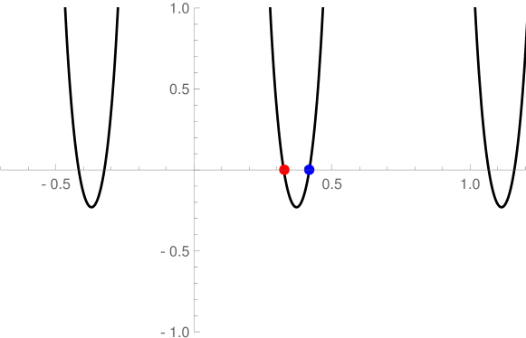
Figure 1: The graph of $y=\wp(x)-\xi^{2}+\delta-a$ under $\psi=\frac{9}{10}\pi$

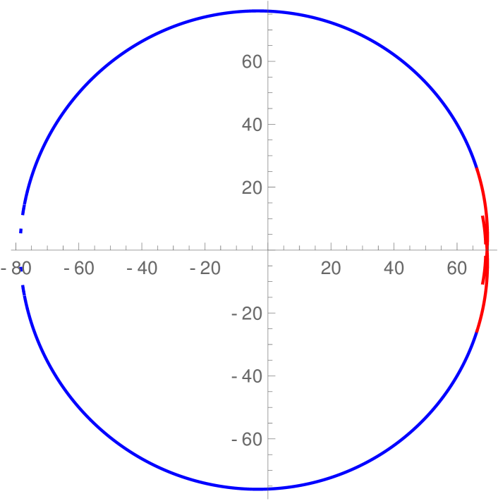
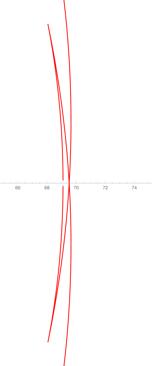
Figure 2: The graph of the front at $t=100$

​​Algorithm

Step-1: We fix the following parameters of the problem: the constants $a=100$, $b=1$ determining the bottom shape and the constant $\xi=0.5$ characterizing the source position.

Step-2: For each fixed $\psi\in[0,\pi]$, there exist infinitely many roots of the equation

$$\wp(p_{\circ})=\xi^{2}-\delta+a.$$ (17)

As $p_{\circ 1}(\psi)$ and $p_{\circ 2}(\psi)$ we take, respectively, the first and second positive roots (see Fig. 1). In the figure, the red point corresponds to $p_{\circ 1}$ and the blue point, to $p_{\circ 2}$. We determine $\varkappa(\psi)$ by the formula (10), where we again take the first positive root.

Remark 2

As already mentioned, the roots of (17) need not be real. We must seek the complex roots in one of the forms $ip_{\circ}$, $p_{\circ}+\omega^{\prime}$, and $ip_{\circ}+\omega$, where $\omega$ is the pure real period of the Weierstrass $\wp$ and $\omega^{\prime}$ is its pure imaginary period, $p_{\circ}$ is real; as $p_{\circ 1}$ and $p_{\circ 2}$ we must again take the first two positive roots.

Step-3: We fix a moment of time $t$. Let $p_{i}(\psi,t)\,(i=1,2)$ be the first positive root of the equation $t=\delta\cdot[p-p_{\circ i}(\psi))-\zeta(p)+\zeta(p_{\circ i}(\psi)]$. If $p_{\circ i}$ is not real, then we seek $p_{i}$ in the same manner as $p_{\circ i}$.

Step-4: For each fixed $t$, we plot the curves in polar coordinates $\varrho,\varphi$, using formulas (9). In the case $\psi\in\left[0,\frac{\pi}{2}\right]$, we take $p_{\circ 1}$ and $p_{1}$ as parameters, and in the case $\psi\in\left[\frac{\pi}{2},\pi\right]$, we take $p_{\circ 2}$ and $p_{2}$.

Step-5: By symmetry, we reflect the obtained graph about the horizontal axis. Figure 2 shows the front at $t=100$; the dashed curve in this figure corresponds to $\psi\in\left[0,\frac{\pi}{2}\right]$ and the solid curve, to $\psi\in\left[\frac{\pi}{2},\pi\right]$.

3 Proof of theorem 1 in a nutshell

Solving the Hamiltonian system (1) with Hamiltonian (7) and initial conditions (8), we get

$$v=\gamma\quad(=\mathrm{const})\,,\quad\left(u^{2}+\frac{\gamma^{2}}{\varrho^{2}}\right)\frac{\varrho^{2}+b}{\varrho^{2}+a}=\frac{\gamma^{2}}{h^{2}}\quad(=\mathrm{const}).$$

Making use of the integral $\mathscr{H}(\varrho,\varphi;u,v)=\gamma/h$, we obtain the following autonomous dynamics for the variable $\varrho$

$$\varrho\,\dot{\varrho}=\frac{\sqrt{(\varrho^{2}+b)\left[\varrho^{2}(\varrho^{2}+a)-(\varrho^{2}+b)h^{2}\right]}}{(\varrho^{2}+a)}\,.$$

Making the change $z=\varrho^{2}+a$ and applying the shift $s=z-\delta$ to reduce the integral to the canonical Weierstrass form

$$\int\limits^{\varrho^{2}+a-\delta}_{\infty}\!\!\!\frac{(s+\delta)\,ds}{\sqrt{4\,s^{3}-\alpha\,s-\beta}}=t,$$

we derive an expression for $\varrho$ in system (9). Using the obtained result and the integral $\mathscr{H}=\gamma/h$, we obtain the formula for $u$. Substituting the obtained expression into the Hamiltonian system, one obtains the equation

$$\dot{\varphi}=h\left(1+\frac{b}{\wp(\boldsymbol{\mathfrak{p}})+\delta-a}\right)\frac{1}{\wp(\boldsymbol{\mathfrak{p}})+\delta}\,.$$

Its integration leads to the logarithmic elliptic integral that can be easily evaluated [8]. Simplifying the obtained expression, we arrive at the solutions (9).

​​Acknowledgments

The authors wish to express their gratitude to S. Yu. Dobrokhotov for the statement of the problem and to M. Babich and M. Pavlov for useful discussions.

References

- [1]
- [2] J. J. Stoker. Waves on Water. The Mathematical Theory with Applications. New York–London, Interscience (1957).
- [3] E. N. Pelinovskii. Hydrodynamics of Tsunami Waves. Nizhnii Novgorod (1996) (in Russian).
- [4] S. Yu. Dobrokhotov, S. Ya. Sekerzh-Zenkovich, B. Tirozzi & B. Volkov. Explicit asymptotics for tsunami waves in framework of the piston model. Russ. J. Earth Sciences (2006) 8(ES403), 1–12.
- [5] S. Yu. Dobrokhotov, A. I. Shafarevich & B. Tirozzi. Localized wave and vortical solutions to linear hyperbolic systems and their application to linear shallow water equations. Russ. J. Math. Phys. (2008) 15(2), 192–221.
- [6] S. Yu. Dobrokhotov & V. E. Nazaikinskii. Asymptotics of localized wave and vortex solutions of a linearized system of shallow water equations. In: Actual Problems of Mechanics (2015), 98–139. Nauka, Moscow (in Russian).
- [7] A. Yu. Anikin, S. Yu. Dobrokhotov, V. E. Nazaikinskii & M. Rouleux. The Maslov canonical operator on a pair of Lagrangian manifolds and asymptotic solutions of stationary with localized right-hand side. Doklady Math. (2017) 96(1), 406–410.
- [8] N. I. Akhiezer. Elements of the Theory of Elliptic Functions. Transl. Math. Monogr. 79. AMS Providence, R. I. (1990).