Identification of gatekeeper diseases on the way to cardiovascular mortality

Abstract

Multimorbidity, the co-occurrence of two or more chronic diseases such as diabetes, obesity or cardiovascular diseases in one patient, is a frequent phenomenon. To make care more efficient, it is of relevance to understand how different diseases condition each other over the life time of a patient. However, most of our current knowledge on such patient careers is either confined to narrow time spans or specific (sets of) diseases. Here, we present a population-wide analysis of long-term patient trajectories by clustering them according to their disease history observed over 17 years. When patients acquire new diseases, their cluster assignment might change. A health trajectory can then be described by a temporal sequence of disease clusters. From the transitions between clusters we construct an age-dependent multilayer network of disease clusters. Random walks on this multilayer network provide a more precise model for the time evolution of multimorbid health states when compared to models that cluster patients based on single diseases. Our results can be used to identify decisive events that potentially determine the future disease trajectory of a patient. We find that for elderly patients the cluster network consists of regions of low, medium and high in-hospital mortality. Diagnoses of diabetes and hypertension are found to strongly increase the likelihood for patients to subsequently move into the high-mortality region later in life.

Noncommunicable (or chronic) diseases (NCDs) such as dorsalgia, hypertension, respiratory diseases or diabetes affect a large fraction of the world’s population and decrease the quality of life of people burdened by them [1]. For example, in 2004, almost $50\%$ of the population of the United States was suffering from at least one chronic condition [2] and in 2014, approximately 25$\%$ of the adults had been diagnosed with more than one NCD [3], with both numbers strongly increasing with age. Besides having a negative impact on people’s wellbeing, NCDs also pose a substantial burden on the healthcare systems of countries [4, 5]. Apart from combatting common risk factors such as unhealthy lifestyle and diet, which many NCDs are attributed to [6], early detection and management play a key role in decreasing the burden of chronic diseases [7]. Personalized (or stratified) medicine promises to make care more efficient by tayloring treatments individually to patients while taking their individual risk profile for potential future diseases into account [8]. A necessary precondition to enter this new era of medicine is a deepened understanding of how the long-term developments of multiple diseases condition each other.

The field of network medicine holds as central tenet that diseases cannot be studied independently from each other but arise from complex interactions between molecular units in the human body in terms of discretized structures such as protein–protein, metabolic, regulatory and RNA networks [9]. For example, the fact that many diseases tend to be comorbid, i.e. that they tend to co-occur in patients, can be understood based on disease-causing genes or pathways shared by the comorbid diseases [10, 11, 12]. However, not all diseases linked by shared genes exhibit significant comorbidities, as different mutations of the same gene can have different consequences. Conversely, not all comorbidities can be explained from molecular data. One reason is that comorbidities can also be the result of the exposure to the same environmental risk factors, for example, due to a particular lifestyle [13]. In addition, present data on molecular interactions is far from being complete [14].

To obtain a more empirically-based understanding of disease comorbidity, observational healthcare data regarding hospital admissions, pharmaceutical prescriptions and doctor visits has been leveraged for the purpose of disease prediction and to reveal previously unknown molecular connections between diseases [15, 16]. Using so-called phenotypic comorbidity networks [17, 18, 19, 20]—networks where nodes represent diseases and two nodes are linked if the two corresponding diseases are comorbid— it was shown that diseases which are comorbid to many other diseases have a higher mortality and that patients tend to develop diseases in close network proximity to the ones they already have. The latter fact opens up the possibility to predict future diseases of patients based on their medical history. This has been accomplished with approaches that include collaborative filtering [21, 22], frequent itemsets [23, 24], learning of transition probabilities between states represented by binary vectors [25, 26], deep learning [27, 28] and point processes [29].

Next to predicting future disease, longitudinal data on hospital admissions allows the identification of previously unknown patterns in the temporal sequence of diseases (health trajectories) patients are diagnosed with. By analyzing the temporal order of diagnosis pairs co-occuring in a significant number of patients with a particular directionality in time, it was possible to identify such trajectories with a length of up to four diseases [30]. Alternative methodological approaches to identify typical health trajectories include dynamic time warping [31], a method originally developed for speech recognition, or the detection of putative causal relations between pairs of diseases using information-theoretic approaches [32]. The major challenge all these works are confronted with is the high number of different diagnosis codes, leading to a combinatorial explosion of the number of possible disease combinations, many of which occur only in a single patient.

Here we present an alternative approach to characterize the population of an entire country in terms of its long-term health trajectories. An illustration of our work flow is shown in fig. 1. First, fig. 1A, we represent the health state of a patient at a given point in time by a binary vector encoding the set of diseases he or she has been diagnosed with so far. Based on a longitudinal data set covering all intramural stays in Austria from 1997 until 2014, see Methods, we consider the yearly disease vectors of all patients without any hospital admission between 1997 and 2002. The set of all health states (disease vectors) is then partitioned using a divisive clustering algorithm called DIVCLUS-T [33], fig. 1B. Each cluster is defined by a set of diseases which each patient in that cluster has been diagnosed with (inclusion criteria) and a set of diseases each patient in that cluster has not been diagnosed with (exclusion criteria). As time proceeds, patients acquire new diseases and consequently can change the cluster they belong to, see fig. 1B. The sequence of clusters a patient belongs to throughout the observation period describes his or her health trajectory. We construct a multiplex network where nodes represent clusters, layers correspond to different patient sex and age groups. Directed links in the multiplex layers are weighted according to the rate at which patients of the corresponding sex and age group change between the two clusters corresponding to the nodes, see fig. 1C. Our approach therefore provides a statistical description of the disease progression of patients which takes into account their sex, age and entire observed history of hospital diagnoses.

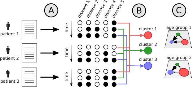
Figure 1: Illustration of the workflow from the input data to a multiplex network model of disease progression. (A) From the input data, we extract the observed health states of patients in the cohort at the end of each year of the observation period, represented by binary vectors. (B) All sampled health states are assigned to clusters using the DIVCLUS-T algorithm. For each patient we thereby obtain a sequence of clusters he or she is assigned to over the years (the health trajectory). (C) From the health trajectories of patients, we construct a multiplex network, where nodes represent clusters, layers represent age and sex groups and directed links between the nodes are weighted according to the rates at which patients change between the corresponding clusters.

1 Results

Our study cohort consists of the $M=5,112,811$ patients who did not receive a diagnosis with ICD-10 code from A00 to N99 in 1997–2002 and received at least one diagnosis with ICD-10 code from A00 to Z99 in 2003–2014. Figure S2 in the Supplementary Information (SI) shows the distribution of the dates of birth of patients of this cohort; 53$\%$ of them are female.

1.1 Disease clusters

For each patient we observe thirteen disease vectors (from the end of each year in the observation period 2002–2014) which are grouped into 132 disease clusters by DIVCLUS-T, see Methods. Tables detailing the inclusion and exclusion criteria of all clusters can be found in SI, section 8. There and in the main text, the symbols ✗ and ✓ next to a diagnosis block indicate that this block is an exclusion, respectively an inclusion criterion for that cluster. Since all patients are free from any (known) prior diagnoses, all patient trajectories start in cluster 0 (the “healthy cluster”), where all diagnoses are exclusion criteria.

In fig. 2(a) we show the sizes, meaning the total number of observations, assigned to each cluster. Note that the cluster IDs are given by their rank after being sorted by size. Color in fig. 2(a) shows the sex distribution within the clusters. There are several clusters only containing patients of one sex; this is explained by sex specific inclusion criteria such as ‘Diseases of male genital organs’ (N40–N51). There are, however, also clusters with a high sex imbalance that is less easily explained. For example, 82$\%$ of the patients in cluster 83 are male. For this cluster, the inclusion criteria are ‘Mental and behavioral disorders due to psychoactive substance use’ (F10–F19) and ‘Diseases of liver’ (K70–K77).

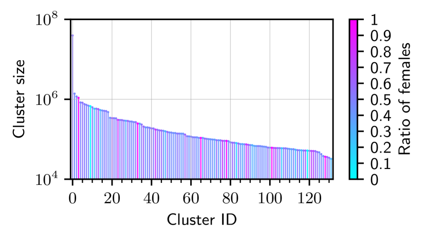
(a)

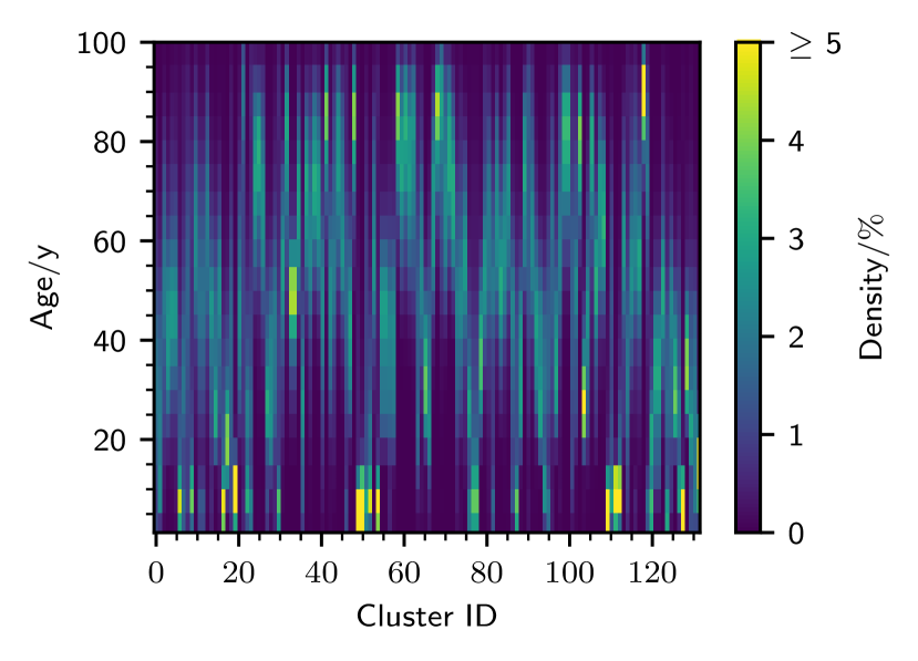
(b)

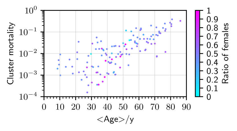
(c)

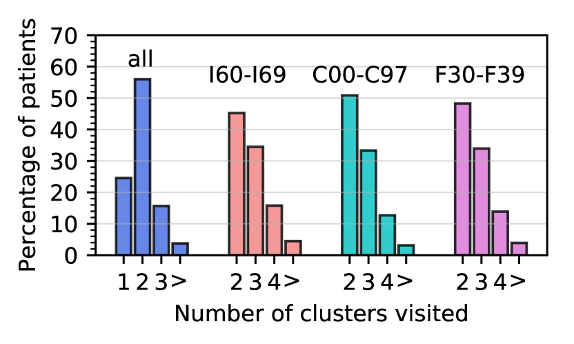
(d)

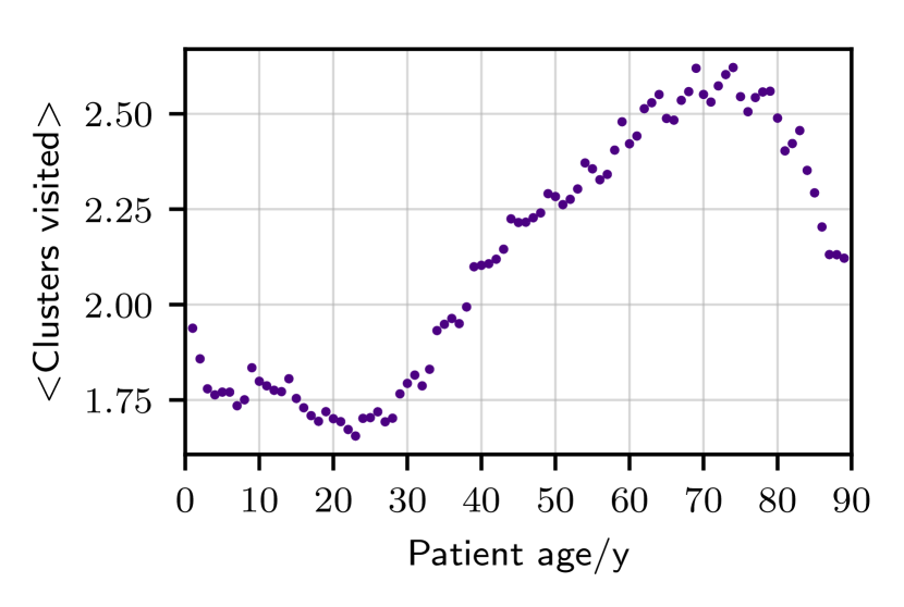
(e)

Cluster 0
all	✗

$\underset{\text{\sf 129,961}}{\longrightarrow}$ Cluster 2 E70-E90 ✗ I10-I15 ✗ I80-I89 ✗ J30-J39 ✗ M00-M25 ✓ M40-M54 ✗ M60-M79 ✗ M80-M94 ✗ $\underset{\text{\sf 5,983}}{\longrightarrow}$ Cluster 31 I10-I15 ✗ J30-J39 ✗ M00-M25 ✓ M60-M79 ✓ M80-M94 ✗

(f)

Figure 2: (A) Number of observations assigned to the different clusters, color coded by the ratio of females in the cluster. (B) Two-dimensional histogram of the age distribution in the different clusters. (C) Scatter plot of mortality versus mean age in the different clusters with color indicating their sex ratios. (D) Relative distribution of the number of clusters visited during the observation period for all people in the cohort (blue), patients diagnosed with cerebrovascular diseases (red, I60–I69), malignant neoplasms (green, C00–C97) and mood [affective] disorders (magenta, F30–F39) during the observation period. (E) Mean number of clusters visited by patients during the observation period depending on their age at the beginning of the observation period. (F) Illustration of the reduced trajectory (0,2,31), which is the most frequent reduced trajectory of length 3 and followed by 5,983 patients of the cohort. The numbers underneath the arrows give the total number of patients who step from cluster 0 to cluster 2 and from cluster 0 to cluster 2 to cluster 31, respectively.

A two-dimensional histogram of the age distributions in the different clusters is shown in fig. 2(b). Clusters differ strongly in their age composition, with a high number of clusters where the distribution is centered around ages 60–80. In fig. 2(c) we compare the mean age of patients in a cluster with the probability that a patient who enters this cluster stays there and dies in-hospital within the observation period (hospital release type death). We refer to this probability as the cluster mortality. Mortality tends to increase with the mean age of patients in a cluster, however, for a given mean age, the spread of the cluster mortality can extend over more than one order of magnitude. The maximum mortality value of 38$\%$ is measured for cluster 68, which has no exclusion criteria and includes hypertensive diseases (I10–I15), other forms of heart disease (I30–I52), diseases of arteries, arterioles and capillaries (I70-I79) and a diagnosis of renal failure (N17–N19). Moreover, 67$\%$ of the health states assigned to that cluster include metabolic disorders (E70-E90) and 49$\%$ include diabetes mellitus (E10-E14).

1.2 Health trajectories

As patients acquire new diseases from one year to the next, they can transition between clusters, see Methods. The time sequence of clusters that a patient has visited defines his or her trajectory. We also define the reduced health trajectory of a patient as the health trajectory with all repetitions removed. For example, if patient $i$ has the health trajectory $(1,1,5,5,5,3)$, then his or her reduced health trajectory is $(1,5,3)$. The blue bars in fig. 2(d) show the distribution of the mean length of the reduced health trajectory of patients during the observation period. Almost 25$\%$ of the patients stay in cluster 0 during the entire time span (only received codes from the ICD chapter O–Z); 2$\%$ visit four or more clusters. Figure 2(e) shows how the length of the reduced health trajectory of patients varies with age. Adolescent patients visit the least number of clusters, and patients around the age of 70 visit the highest number of clusters. The most frequent reduced trajectory of length 3 is (0,2,31), and is followed by 5,983 individuals; fig. 2(f). Patients with this reduced trajectory first acquire a diagnosis from the block ‘Arthropathies’ (M00–M25) and subsequently one from the block ‘Soft tissue disorders’ (M60–M79).

We now describe results for typical health trajectories involving the diagnosis blocks of ‘Cerebrovascular diseases’, ‘Malignant neoplasms’ and ‘Mood [affective] disorders’.

Cerebrovascular diseases (I60–I69). A total of 199,681 patients (3.9$\%$) were diagnosed with cerebrovascular diseases. The distribution of the length of their reduced trajectories is clearly shifted towards higher values compared to the total cohort; see fig. 2(d). The most frequent reduced trajectory of length three, followed by 1,447 patients, is (0,32,48), meaning that patients from the “healthy cluster” 0 (all diseases are exclusion criteria) move to cluster 32 with hypertensive diseases (I10–I15) and heart diseases (I30–I52) to cluster 48 where cerebrovascular diseases (I60–I69) changed from an exclusion (cluster 32) to an inclusion criterion (cluster 48).

Malignant neoplasms (C00–C97). A total of 312,787 patients (6.1$\%$) received a diagnosis from the block ‘Malignant neoplasms’. The distribution of the number of visited clusters visited by these patients is shown in fig. 2(d) and shifted toward higher values with respect to all other patients. More than $50\%$ of them only visit two different clusters, and $44\%$ (69,552) of those patients have the reduced trajectory (0,12), i.e., from the healthy cluster to a cluster where cancer (C00–C97) is the only inclusion criterion. The most frequent reduced trajectory of length 3, followed by 3,093 cancer patients, is (0,12,38) where patients acquire hypertensive diseases (I10–I15) after cancer.

Mood [affective] disorders (F30–F39). A total of 210,589 patients (4.1$\%$) of the study cohort are diagnosed with mood or affective disorders during the observation period. The distribution of their reduced trajectory lengths is shown in fig. 2(d) and again shifted toward higher lengths compared to all patients. Among these patients, 9.5$\%$ end their trajectory in cluster 55, where additional to ‘Mood [affective] disorders’, patients are diagnosed with a diagnosis from the block ‘Mental and behavioral disorders due to psychoactive substance use’ (F10–F19). The most common reduced trajectory of length 3 in this subcohort, followed by 1,936 patients, is (0,14,55). These patients first acquire a diagnosis from the block F10–F19, and subsequently one from the block F30–F39.

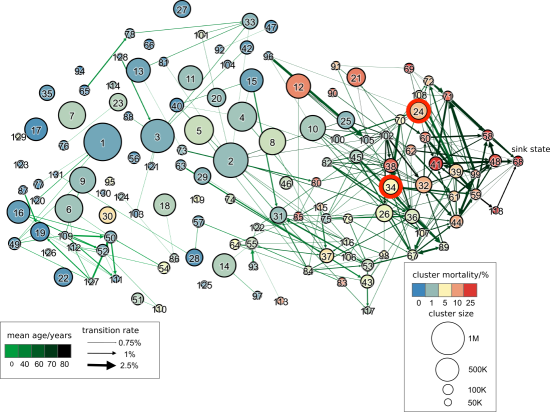
Figure 3: Plot of the collapsed dynamic network $\mathcal{M}$, where nodes represent clusters and directed edges between the nodes are weighted according to the transition probability between the two nodes. The edges are colored depending on the mean age of the patients who make the corresponding step. Light green edges indicate a low mean age and dark green edges indicate a high mean age of the patients making the corresponding step. The size of the nodes is scaled according to the size of the corresponding cluster and the node color indicates the cluster mortality, with blue indicating low mortality and red indicating high mortality. The node representing cluster 0, which is connected to all other nodes, has been removed in this visualization. The layout has been generated by a force-directed algorithm after which nodes have been displaced from left to right by a distance proportional to the average age associated with its links, i.e., patient age increases from left to right. To increase the readability, we only display the 255 strongest links of the network. For elderly patients we observe network regions of low, medium and high mortality. Clusters 24 and 34, which are identified as gatekeepers to the sink state, are marked with red circles; the sink state cluster 68 is annotated.

1.3 Disease cluster multiplex network

Separately for males and females, we construct a directed multiplex dynamic network, $\mathcal{M}$, where nodes represent patient clusters and layers (time slices) correspond to age and sex groups. A directed link from node $i$ to node $j$ within time slice $a$ in the network for patients of sex $g$ has a weight proportional to the number of observed transitions from cluster $i$ to $j$ of patients with corresponding age and sex. Figure 3 shows a visualization of the dynamic network of clusters of patient health states, filtered and collapsed into one layer. Nodes correspond to clusters and their size is the number of observations in that cluster; node color corresponds to cluster mortality on a scale from 0% (blue) to 38% (red). Links indicate a significant number of transitions between two clusters of patients with an average age that is encoded into the link color from 0y (light green) to 80y (black). The layout in fig. 3 has been generated in a force-directed way, after which the nodes were displaced from left to right by a distance proportional to the average age of patients in the cluster. As patients age (move from left to right in the network), they either reach a region of low or high mortality. The low mortality clusters for the elderly (clusters 25, 102, 105) are characterized by having various diseases of the eye as inclusion criteria and most other diseases as exclusion criteria. Contrast this to the high mortality region for the elderly that is often accessed via cluster 24 (including hypertensive, I10–I15, and diabetes, E10-E14) or cluster 26 (with hypertensive diseases and metabolic disorders, E70–E90). Cluster 68 is a sink state of our dynamic multiplex network, i.e. has zero out-strength, and lies within the high-mortality region. Note that the fact that there exists such a sink state is a consequence of our choice of clustering algorithm. There are clusters for younger patients with links pointing toward the low and high mortality regions, such as cluster 2 (including arthropathies, M00–M25) or cluster 29 (diseases of the oesophagus, stomach, and duodenum, K20–K31). While cluster 68 has a balanced sex ratio (49% females), many clusters with direct links to 68 have an overrepresentation of females (65% in cluster 118, 52% in 58, 59% in 48). Additionally, we find a region of medium mortality for the elderly made up of clusters that include arthropathies and osteopathies (M80–M94), cluster 43, or additionally soft tissue disorders (M60–M79), cluster 117.

1.4 Gatekeeper clusters

We identify “gatekeeper clusters” strongly increasing the risk of cardiovascular mortality by using a stochastic model of disease progression. Precisely, we model health trajectories as random walks on the disease cluster multiplex network $\mathcal{M}$, see Methods.

For a given cluster $k$, we term as gatekeepers to $k$ those clusters which tend to be visited by many patients early in their medical career and where patients visiting that cluster have, according to our random walk model, an increased probability to visit cluster $k$ during their lifetime. For the high-mortality cluster 68 (the sink state), we identify cluster 24 as a gatekeeper, highlighted red in fig. 3; see SI for details. Patients in that cluster necessarily have been diagnosed with diabetes mellitus (E10-E14) and hypertensive diseases (I10-I15), but have not yet received diagnoses of obesity and other hyperalimentation (E65-E68), metabolic disorders (E70-E90) and other forms of heart disease (I30-I52). The probability that a patient of the cohort who enters into cluster 24 will reach cluster 68 during his or her lifetime according to our model is 0.23, and is hence increased by approx. $40\%$ compared to the baseline probability of 0.16 for all patients of the cohort. Another closely related gatekeepers is clusters 34 (metabolic, hypertensive, and ischaemic heart diseases but no diabetes and no other forms of heart diseases), for which the probability to reach cluster 68 increases by approx. 50–60%. Clusters 34 is also highlighted red in fig. 3.

2 Discussion

We presented a novel method to describe patient trajectories as observed over 17y from a population-wide data set on hospital diagnoses. The method is based on partitioning observed medical histories of patients into a small number of clusters. A statistical analysis of the transition rates between clusters enabled us to create a model which can be used to simulate synthetic patient trajectories as random walks on a multiplex network.

We show that elderly patients can be found in regions of low, medium and high mortality. The high mortality region is characterized by the co-occurrence of multiple chronic conditions ranging from diabetes, cardiovascular diseases, coronary heart disease, to renal failure; most of these diseases are exclusion criteria in the low mortality region for the elderly, where they only suffer from diseases such as senile cataract. Although morbidity and mortality attributable to cardiovascular diseases decreased in the last decade (with greater improvement in men), they remain the predominant causes of mortality in both sexes. On the other hand NCDs like obesity, metabolic disorders, diabetes and renal diseases increased in men and women, partly due to population aging. The comorbid prevalence of diabetes and renal disease and failure markedly increases cardiovascular morbidity and mortality. Patients with renal diseases hardly achieve the targets for blood pressure and glycemic control. However, the use of new classes of antidiabetic drugs may change the paradigm of ineluctable cardiorenal risk in the future [34].

Some patients enter the region of high mortality and high disease burden at an older age via the low mortality region in fig. 3. For others, however, the course toward high mortality is already set at much younger ages. For instance, cluster 46 consists of patients with an average age of 44y, metabolic disorders (E70–E90) and about thirty other diagnosis blocks as exclusion criteria. From this cluster there is a link to cluster 34 where patients additionally receive diagnoses of hypertensive and ischaemic heart diseases, after which disease and mortality burden are bound to increase further. This is in line with findings that patients with metabolic syndrome have an almost threefold increased mortality because of cardiovascular or coronary heart disease in an 11.4y follow up [35]. In this sense, patients with metabolic disorders appear to be locked in on a path toward high mortality already at much younger age (say, between 40y and 50y).

We identified several gatekeeper clusters that can be loosely seen as “points of no return” toward the high mortality network region. By identifying how patients transition into these gatekeeper clusters, we find that diabetes mellitus and hypertension often stand at the beginning of the medical career of patients. These diseases substantially increase their probability to subsequently move into the high-mortality region of the cluster network. Diabetes and hypertension are the most prominent risk factors for development of both renal failure and cardiovascular disease. Unfortunately, they are often undetected and only diagnosed because of acute complications caused by the underlying disorders. For example, in Denmark 35% of the patients with newly diagnosed diabetes featured diabetic complications around diagnosis [36]. As patients usually suffer from diabetes for many years before the diagnosis, screening and prevention programmes are necessary at least for subjects at high risk. It is highly recommended that patients with the clinical features hypertension, vascular diseases, dyslipidemia, prediabetes or abdominal obesity, often clustering as “metabolic syndrome”, should as early as possible and all (other) subjects older than 45 years undergo diabetes screening at regular intervals [37]. Such procedure could help to identify more patients at risk earlier and to implement secondary prevention of long-term complications and assure guidelines-based therapy.

Females are overrepresented in several clusters with direct links to the high-mortality cluster 68, which in itself has a balanced sex ratio. Both diabetes and renal failure appear to attenuate the generally positive effect of female sex on life expectancy: these disorders seem to increase risk in women to a greater extent, thereby equalizing mortality risks [38, 39, 40]. This may be ascribed to sex-dimorphic changes in risk factor burden and enviromental factors. Among patients with type 2 diabetes, which comprises more than 90% of all diabetes cases, women with type 2 diabetes were shown to be more likely obese, hypertensive and to have hypercholesterolaemia but were less likely to be prescribed lipid-lowering medication and antihypertensive drugs, especially if they had cardiovascular disease in comparison to men [41]. Moreover it was shown that admissions for acute myocardial infarctions steadily increased in the last two decades especially in younger patients whose history of diabetes and hypertension increased in parallel [42]. The proportion attributable to younger women was particularly high who also had lower probability of receiving guideline-directed therapy.

Limitations of this work include that we do not know the health history of patients prior to the observation period. Also, the data only contains health information from hospital stays but not from outpatient contacts or doctor visits. Moreover, the fact that the data was originally recorded for billing purposes means that diagnoses which do not lead to financial reimbursement were often not reported. The actual disease burden of patients might therefore be underrepresented in our data. Simulated trajectories might occur that are logically not possible. The model might produce a patient trajectory starting in cluster $A$, with disease $d$ as an inclusion criterion, stepping to cluster $B$, where $d$ is neither an exclusion nor an inclusion criterion, and from there to cluster $C$, where $d$ is now an exclusion criterion. To assess the quality of the trajectory model, we compared our results with different benchmark models that assign patients to clusters based on single diseases (either the most recent or least frequent one) rather than using exclusion criteria. These benchmarks perform either comparable or only slightly worse than the DIVCLUS-T approach in terms of cluster inertia. This can be understood from the fact that the benchmark models nevertheless capture disease–disease correlations (note that for a given cluster, the cluster-specific frequencies of other diseases are the marginal frequencies of the diseases computed over all patients fulfilling the criteria for that cluster). However, if we take the longitudinal component of the data into account and compare the statistics of simulated and real patient trajectories, we find that our approach clearly outperforms the benchmark models. This confirms that the issue of logically impossible trajectories does not substantially impact our results. In addition, these results reveal that our multiplex network approach based on multimorbidity clusters provides a more adequate framework to capture the path-dependent nature of long-term health trajectories compared to the single-disease benchmark models. It will be of interest to extend the current framework with additional clinical variables or to focus on more specific subsets of patients for a more precise identification of disease gatekeepers.

Data and Methods

A Data

We analyze a data set provided by the Austrian Federal Ministry for Health, covering all approx. 45M hospital stays of about 9M individuals in Austria during the 17 years from 1997 until 2014. Here, the term hospital also includes facilities of long-term care such as rehabilitation centers or psychiatric hospitals [43]. For each stay of a patient, the data includes sex, age group (5y interval), admission and release date, release type (release, transfer, death), as well as in total about 120M main or side diagnoses in the form of level-3 ICD-10 codes [44]. We restrict our analysis to 1,074 codes from A00 to N99, as the remaining codes relate to medical conditions that do not necessarily reflect diseases. Due to the similarity of the conditions described by many codes, we group them into 131 blocks as defined by the WHO. For example, the codes from E10 to E14 form the block ‘Diabetes Mellitus’. A list of all diagnosis blocks can be found in section 9 of the Supporting Information (SI) to this article. To make sure that the patients are in a well defined health state at the beginning of the observed time period, we restrict the analysis to all patients not assigned a diagnosis from the range A00 to N99 during a hospital stay in Austria in the period from 1997 to 2002 inclusively.

B Clustering

The (observed) health state of a patient at a given point in time consists of all diseases he or she has been diagnosed with until that point. We represent the health state of a patient $i$ ($1\leq i\leq M$) at time $t$ by a binary vector $\mathbf{x}^{(i)}(t)=(x_{1}^{(i)}(t),\dots,x_{N}^{(i)}(t))$, where $N$ denotes the total number of disease codes, and $x_{j}^{(i)}(t)$ is one if patient $i$ has been diagnosed with disease $j$ until time $t$ and zero else.We choose a set of equidistant time values $T=\{t_{0},\dots,t_{n}\}$, where $t_{i+1}-t_{i}=\Delta~{}(1\leq i<n)$, at which we sample the health state of each patient. The parameter $\Delta$ controls the temporal resolution of the analysis. The values $t_{0}$ and $t_{n}$ mark the start and end point of the observation period, respectively.

We use a divisive clustering algorithm called DIVCLUS-T [33], to partition the set of observed health states of patients with at least one diagnosis into $K=131$ clusters; see SI, section 2. An additional cluster contains all health states of patients who did not receive any diagnose yet. The DIVCLUS-T algorithm aims to minimize the same objective function as the well-known Ward’s method and the $k$-means algorithm, but produces results which are easier to interpret. More precisely, each cluster is defined by a set of diseases which all patients in that cluster have been diagnosed with and a set of diseases which all patients in that cluster have not been diagnosed with. We refer to these sets as the inclusion, respectively the exclusion criteria for that cluster.

C Analysis of cluster transitions

Denote for $t\in T$ by $C_{i}(t)$ the cluster to which observation $\mathbf{x}^{(i)}(t)$ is assigned. The sequence $\mathcal{S}_{i}=(C_{i}(t_{0}),\dots,C_{i}(t_{n}))$ describes the health trajectory of patient $i$ throughout the observation period. We also define the reduced health trajectory of a patient as the health trajectory with all repetitions removed. If for a given $1\leq i\leq M$ and $1\leq s<n$, $C_{i}(t_{s})=k$ and $C_{i}(t_{s+1})=j$, then we say that patient $i$ steps from cluster $k$ to cluster $j$. For each pair of clusters $1\leq k,j\leq K$, there exists at least one disease which is an exclusion criterion in one and an inclusion criterion in the other cluster. Since we represent patients by all diseases which they have been diagnosed with so far, a patient cannot step from a cluster in which a certain disease is an inclusion criterion to one where this disease is an exclusion criterion, and therefore, steps between two clusters are only possible in one direction.

The cohort is stratified into groups according to sex and age. For a given sex $g$ and age group $a$, we define $s_{g,a,k,j}$ as the number of patients of sex $g$ and age group $g$ who step from cluster $k$ to cluster $j$; the value

$$q_{g,a,k,j}=\frac{s_{g,a,k,j}}{\sum_{j=1}^{K}s_{g,a,k,j}}$$ (1)

is the rate at which patients of this sex and age group make this step.

D Modeling health trajectories

To simulate the future trajectory of a patient, we first determine his or her starting position according to age and history of medical diagnoses. Let at time $t_{0}$ the patient be in cluster $k$ on time slice $a$ of the network. Then we randomly choose the position of this patient at time $t_{1}=t_{0}+\Delta$, such that with probability $q_{g,a^{\prime},k,j}$, his or her next position is in cluster $j$ on time slice $a^{\prime}$; the time slice $a^{\prime}$ is determined from the age of the patient at time $t_{1}$. To compare results of our method to simulate random health trajectories with the health trajectories observed, we simulate as many synthetic health trajectories as there are patients in our study cohort, with the same sex and age distribution as our cohort. The initial condition of the model is taken from the data, i.e., all patients start their trajectory in the “healthy” cluster where all diseases are exclusion criteria (cluster zero). To assess the quality of the simulated health trajectories, we compute several metrics for comparing disease frequencies according to the simulated trajectories with the data, and compare the performance of our method in terms of these metrics with two benchmark models, see SI. Fig. S4 (b) in the SI shows the forecasted distribution of patients of the study cohort over the different clusters at the end of their lives.

Author Contributions

N.H. and P.K. conceived the study and devised the analytic methods, N.H. wrote the manuscript with contributions from P.K. and A.K.-W., N.H. carried out the analysis and produced plots and graphics, S.T. made critical comments regarding the manuscript, A.K.-W. contributed expertise regarding the medical interpretation of the findings, M.G., P.K. and N.H. researched and prepared the data. All authors read and approved the manuscript.

See pages - of SI_dis_traj.pdf

References

- [1] World Health Organization, “Noncommunicable diseases. Fact sheet.” https://www.who.int/en/news-room/fact-sheets/detail/noncommunicable-diseases, retrieved 5 Dec 2018.
- [2] Robert Wood Johnson Foundation Partnership for Solutions, “Chronic conditions: Making the case for ongoing care.” https://www.rwjf.org/en/library/research/2004/09/chronic-conditions-.html, 2004.
- [3] B. Ward and L. Black, “State and regional prevalence of diagnosed multiple chronic conditions among adults aged 18 years — United States, 2014,” MMWR Morb Mortal Wkly Rep, vol. 65, p. 735–738, 2016.
- [4] M. Mueller and D. Morgan, “Spending on health: Latest trends.” http://www.oecd.org/health/health-systems/Health-Spending-Latest-Trends-Brief.pdf, 2018.
- [5] D. M. Berwick and A. D. Hackbarth, “Eliminating waste in us health care,” Journal of the American Medical Association, vol. 307, pp. 1513–1516, April 2012.
- [6] G. Danaei, E. L. Ding, D. Mozaffarian, B. Taylor, J. Rehm, C. J. L. Murray, and M. Ezzati, “The preventable causes of death in the united states: Comparative risk assessment of dietary, lifestyle, and metabolic risk factors,” PLoS Medicine, vol. 6, p. e1000058, April 2009.
- [7] A. M. El Nahas and A. K. Bello, “Chronic kidney disease: the global challenge,” Lancet, vol. 365, pp. 331–340, 2005.
- [8] Personalized Medicine Coalition, “The case for personalized medicine.” http://www.personalizedmedicinecoalition.org/Userfiles/PMC-Corporate/file/pmc_case_for_personalized_medicine.pdf, 2014.
- [9] A.-L. Barabási, N. Gulbahce, and J. Loscalzo, “Network medicine: A network-based approach to human disease,” Nature Reviews Genetics, vol. 12, pp. 56–68, 2012.
- [10] K.-I. Goh, M. E. Cusick, D. Valle, B. Childs, M. Vidal, and A.-L. Barabási, “The human disease network,” PNAS, vol. 104, no. 21, pp. 8685–8690, 2007.
- [11] A. Rzhetsky, D. Wajngurt, N. Park, and T. Zheng, “Probing genetic overlap among complex human phenotypes,” Proceedings of the National Academy of Sciences, vol. 28, pp. 11694–11699, July 2007.
- [12] J. Park, D.-S. Lee, N. A. Christakis, and A.-L. Barabási, “The impact of cellular networks on disease comorbidity,” Molecular Systems Biology, vol. 5, no. 262, 2009.
- [13] P. Klimek, S. Aichberger, and S. Thurner, “Disentangling genetic and environmental risk factors for individual diseases from multiplex comorbidity networks,” Scientific Reports, vol. 6, no. 39658, 2016.
- [14] J. Menche, A. Sharma, M. Kitsak, S. D. Ghiassian, M. Vidal, J. Loscalzo, and A.-L. Barabási, “Uncovering disease-disease relationships through the incomplete interactome,” Science, vol. 347, no. 1257601, 2015.
- [15] P. B. Jensen, L. J. Jensen, and S. Brunak, “Mining electronic health records: towards better research applications and clinical care,” Nature Reviews Genetics, vol. 13, pp. 395–405, 2012.
- [16] S. Schneeweiss, “Learning from big health care data,” New England Journal of Medicine, p. 3, 2014.
- [17] C. A. Hidalgo, N. Blumm, A. L. Barabási, and N. A. Christakis, “A dynamic network approach for the study of human phenotypes,” PLoS Computational Biology, vol. 5, no. 4, p. 11, 2009.
- [18] A. Chmiel, P. Klimek, and S. Thurner, “Spreading of diseases through comorbidity networks across life and gender,” New Journal of Physics, vol. 16, 2014.
- [19] E. Jeong, K. Ko, S. Oh, and H. W. Han, “Network-based analysis of diagnosis progression patterns using claims data,” Scientific Reports, vol. 7, no. 15561, 2017.
- [20] B. Fotouhi, N. Momeni, M. A. Riolo, , and D. L. Buckeridge, “Statistical methods for constructing disease comorbidity networks from longitudinal inpatient data,” Applied Network Science, vol. 3, no. 46, 2018.
- [21] D. A. Davis, N. V. Chawla, N. Blumm, N. Christakis, and A.-L. Barabási, “Predicting individual disease risk based on medical history,” Proceedings of the 17th ACM conference on Information and knowledge mining - CIKM ’08, pp. 769–778, 2008.
- [22] K. Steinhaeuser and N. V. Chawla, “A network-based approach to understanding and predicting diseases,” in Social Computing and Behavioral Modeling, Springer, Boston, MA, 2009.
- [23] F. Folino, C. Pizzuti, and M. Ventura, “A comorbidity network approach to predict disease risk,” in Information Technology in Bio- and Medical Informatics, ITBAM 2010 (S. Khuri, L. Lhotská, and N. Pisanti, eds.), vol. 6266 of Lecture notes in Computer Science, Springer, Berlin, Heidelberg, 2010.
- [24] F. Folino and C. Pizzuti, “A recommendation engine for disease prediction,” Information Systems and e-Business Management, vol. 13, no. 4, pp. 609–628, 2015.
- [25] O. Arandjelović, “Discovering hospital admission patterns using models learnt from electronic hospital records,” Bioinformatics, vol. 31, no. 24, pp. 3970–3976, 2015.
- [26] I. Vasiljeva and O. Arandjelović, “Diagnosis prediction from electronic health records using the binary diagnosis history vector representation,” Journal of Computational Biology, vol. 24, no. 8, pp. 767–786, 2017.
- [27] T. Pham, T. Tran, D. Phung, and S. Venkatesh, “Deepcare: A deep dynamic memory model for predictive medicine,” in Advances in Knowledge Discovery and Data Mining (J. Bailey, L. Khan, T. Washio, G. Dobbie, and R. W. J. Huang, eds.), vol. 9652 of Lecture Notes in Computer Science, Springer, Cham, 2016.
- [28] R. Miotto, L. Li, B. A. Kidd, and J. T. Dudley, “Deep patient: An unsupervised representation to predict the future of patients from the electronic health records,” Scientific Reports, vol. 6, no. 26094, 2016.
- [29] J. C. Weiss and D. Page, “Forest-based point process for event prediction from electronic health records,” in Machine Learning and Knowledge Discovery in Databases (H. Blockeel, K. Kersting, S. Nijssen, and F. Železný, eds.), pp. 547–562, 2013. Part III.
- [30] A. B. Jensen, P. L. Moseley, T. I. Oprea, S. G. Ellesøe, R. Eriksson, H. Schmock, P. B. Jensen, L. J. Jensen, and S. Brunak, “Temporal disease trajectories condensed from population-wide registry data covering 6.2 million patients,” Nature Communications, vol. 5, no. 4022, 2014.
- [31] A. Giannoula, A. Gutierrez-Sacristán, Á. Bravo, F. Sanz, and L. I. Furlong, “Identifying temporal patterns in patient disease trajectories using dynamic time warping: A population-based study,” Scientific Reports, vol. 8, no. 4216, 2018.
- [32] V. Kannan, F. Swartz, N. A. Kiani, G. Silberberg, G. Tsipras, D. Gomez-Cabrero, K. Alexanderson, and J. Tegnèr, “Conditional disease development extracted from longitudinal health care cohort data using layered network construction,” Scientific Reports, vol. 6, no. 26170, 2016.
- [33] M. Chavent, Y. Lechevallier, and O. Briant, “DIVCLUS-T: A monothetic divisive hierarchical clustering method,” Computational Statistics and Data Analysis, vol. 52, no. 2, pp. 687–701, 2007.
- [34] D. Giugliano, J. J. Meier, and K. Esposito, “Heart failure and type 2 diabetes: From cardiovascular outcome trials, with hope,” Diabetes, Obesity and Metabolism, vol. 21, pp. 1081–1087, 2019.
- [35] H. Lakka, D. Laaksonen, T. Lakka, L. Niskanen, E. Kumpusalo, J. Tuomilehto, and J. Salonen, “The metabolic syndrome and total and cardiovascular disease mortality in middle-aged men,” JAMA, vol. 288, no. 21, pp. 2709–2716, 2002.
- [36] A. Gedebjerg, T. Almdal, K. Berencsi, J. Rungby, J. Nielsen, D. Witte, S. Friborg, I. Brandslund, A. Vaag, H. Beck-Nielsen, H. Sørensen, and R. Thomsen, “Prevalence of micro- and macrovascular diabetes complications at time of type 2 diabetes diagnosis and associated clinical characteristics: A cross-sectional baseline study of 6958 patients in the Danish DD2 cohort,” Journal of Diabetes and its Complications, vol. 32, no. 1, pp. 34–40, 2018.
- [37] American Diabetes Association, “Introduction: Standards of medical care in diabetes–2019,” Diabetes Care, vol. 42, Jan. 2019.
- [38] A. Kautzky-Willer, J. Harreiter, and G. Pacini, “Sex and gender differences in risk, pathophysiology and complications of type 2 diabetes mellitus,” Endocrine Reviews, vol. 37, pp. 278–316, 06 2016.
- [39] J. G. Regensteiner, S. Golden, A. G. Huebschmann, E. Barrett-Connor, A. Y. Chang, D. Chyun, C. S. Fox, C. Kim, N. Mehta, J. F. Reckelhoff, J. E. Reusch, K. M. Rexrode, A. E. Sumner, F. K. Welty, N. K. Wenger, and B. Anton, “Sex differences in the cardiovascular consequences of diabetes mellitus,” Circulation, vol. 132, pp. 2424–2447, 2015.
- [40] M. Hecking, B. A. Bieber, J. Ethier, A. Kautzky-Willer, G. Sunder-Plassmann, M. D. Säemann, S. P. B. Ramirez, B. W. Gillespie, R. L. Pisoni, B. M. Robinson, and F. K. Port, “Sex-specific differences in hemodialysis prevalence and practices and the male-to-female mortality rate: The dialysis outcomes and practice patterns study (dopps),” PLOS Medicine, vol. 11, pp. 1–17, 10 2014.
- [41] A. K. Wright, E. Kontopantelis, R. Emsley, I. E. Buchan, M. A. Mamas, N. Sattar, D. M. Ashcroft, and M. K. Rutter, “Cardiovascular risk and risk factor management in type 2 diabetes: A population-based cohort study assessing sex disparities,” Circulation, 2019.
- [42] S. Arora, G. A. Stouffer, A. M. Kucharska-Newton, A. Qamar, M. Vaduganathan, A. Pandey, D. Porterfield, R. Blankstein, W. D. Rosamond, D. L. Bhatt, and M. C. Caughey, “Twenty year trends and sex differences in young adults hospitalized with acute myocardial infarction,” Circulation, vol. 139, pp. 1047–1056, 2019.
- [43] “Krankenanstalten in Österreich.” https://www.sozialministerium.at/site/Gesundheit/Gesundheitssystem/Krankenanstalten/Krankenanstalten_und_selbststaendige_Ambulatorien_in_Oesterreich/Krankenanstalten_in_Oesterreich, 2019. Accessed 08 February 2019.
- [44] World Health Organization, “International Statistical Classification of Diseases and Related Health Problems 10th Revision.” https://icd.who.int/browse10/2016/en, 2016.