A tutorial-driven introduction to the parallel finite element library FEMPAR v1.0.0

Abstract.

This work is a user guide to the FEMPAR scientific software library. FEMPAR is an open-source object-oriented framework for the simulation of partial differential equations (PDEs) using finite element methods on distributed-memory platforms. It provides a rich set of tools for numerical discretization and built-in scalable solvers for the resulting linear systems of equations. An application expert that wants to simulate a PDE-governed problem has to extend the framework with a description of the weak form of the PDE at hand (and additional perturbation terms for non-conforming approximations). We show how to use the library by going through three different tutorials. The first tutorial simulates a linear PDE (Poisson equation) in a serial environment for a structured mesh using both continuous and discontinuous Galerkin finite element methods. The second tutorial extends it with adaptive mesh refinement on octree meshes. The third tutorial is a distributed-memory version of the previous one that combines a scalable octree handler and a scalable domain decomposition solver. The exposition is restricted to linear PDEs and simple geometries to keep it concise. The interested user can dive into more tutorials available in the FEMPAR public repository to learn about further capabilities of the library, e.g., nonlinear PDEs and nonlinear solvers, time integration, multi-field PDEs, block preconditioning, or unstructured mesh handling.

Keywords: Mathematical Software, Finite Elements, Object-Oriented Programming, Partial Differential Equations

1. Introduction

This work is a user-guide introduction to the first public release, i.e., version 1.0.0, of the scientific software FEMPAR. FEMPAR is an Object-Oriented (OO) framework for the numerical approximation of Partial Differential Equations using Finite Elements. From inception, it has been designed to be scalable on supercomputers and to easily handle multiphysics problems. FEMPAR v1.0.0 has about 300K lines of code written in (mostly) OO Fortran using the features defined in the 2003 and 2008 standards of the language. FEMPAR is publicly available in the Git repository https://github.com/fempar/fempar.

FEMPAR FE technology includes not only arbitrary order Lagrangian FEs, but also curl- and div-conforming ones. The library supports n-cube and n-simplex meshes. Continuous and discontinuous spaces can be used, providing all the machinery for the integration of Discontinuous Galerkin (DG) terms on facets. It also provides support for dealing with hanging nodes in non-conforming meshes resulting from $h$-adaptivity. In all cases, FEMPAR provides mesh partitioning tools for unstructured meshes and parallel octree handlers for $h$-adaptive simulations (relying on p4est [1]), together with algorithms for the parallel generation of FEs spaces (e.g., global numbering of Degrees Of Freedom across processors).

FEMPAR has been applied to a broad set of applications that includes the simulation of turbulent flows [2, 3, 4, 5], magnetohydrodynamics [6, 7, 8, 9, 10], monotonic FEs [11, 12, 13, 14, 15], unfitted FEs and embedded boundary methods [16, 17], additive manufacturing simulations [18, 19, 20], and electromagnetics and superconductors [21, 22].

FEMPAR includes a highly scalable built-in numerical linear algebra module based on state-of-the-art domain decomposition solvers; the multilevel Balancing Domain Decomposition by Constraints (BDDC) solver in FEMPAR has scaled up to 1.75 million MPI tasks in the JUQUEEN Supercomputer [23, 24]. This linear algebra framework has been designed to efficiently tackle the linear systems that arise from FE discretizations, exploiting the underlying mathematical structure of the PDEs. It is a difference with respect to popular multi-purpose linear algebra packages like PETSc [25], for which FEMPAR also provides wrappers. The library also supplies block preconditioning strategies for multiphysics applications [26]. The numerical linear algebra suite is very customizable and has already been used for the implementation and scalability analysis of different Domain Decomposition (DD) solvers [27, 23, 28, 24, 29, 30, 31, 32, 33, 34, 35] and block preconditioners for multiphysics applications [36].

The design of such a large numerical library is a tremendous task. A comprehensive presentation of the underlying design of the building blocks of the library can be found in [37]. This reference is more oriented to FEMPAR developers that want to extend or enhance the library capabilities. Fortunately, users whose application requirements are already fulfilled by FEMPAR do not require to know all these details, which can certainly be overwhelming. In any case, [37, Sect. 3] can be a good introduction to the main abstractions in a FE code.

Even though new capabilities are steadily being added to the library, FEMPAR is in a quite mature state. Minor changes on the interfaces relevant to users have been made during the last two years. It has motivated the recent public release of its first stable version and the elaboration of this user guide.

This user guide is tutorial-driven. We have designed three different tutorials covering an important part of FEMPAR capabilities. The first tutorial addresses a Poisson problem with a known analytical solution that exhibits an internal layer. It considers both a continuous FE and a Interior Penalty (IP) DG numerical discretization of the problem. The second tutorial builds on the first one, introducing an adaptive mesh refinement strategy. The third tutorial consists in the parallelization of the second tutorial for distributed-memory machines and the set up of a scalable BDDC preconditioner at the linear solver step.

In order to keep the presentation concise, we do not aim to be exhaustive. Many features of the library, e.g., the set up of time integrators and nonlinear solvers or multiphysics capabilities, have not been covered here. Instead, we encourage the interested reader to explore the tutorials section in the Git repository https://github.com/fempar/fempar, where one can find the tutorials presented herein and other (more advanced) tutorials that make use of these additional tools.

2. Brief overview of FEMPAR main software abstractions

In this section, we introduce the main mathematical abstractions in FE problems that are provided by FEMPAR. In any case, we refer the reader to [37, Sect. 3.1] for a more comprehensive exposition. Typically, a FEMPAR user aims to approximate a (system of) PDEs posed in a bounded physical domain $\Omega$ stated in weak form as follows: find $u_{g}\in V_{g}$ such that

(1) $${a}(u_{g},v)=\ell(v),\,\qquad\hbox{for any }v\in V,$$

where ${a}(u,v)$ and $\ell(v)$ are the corresponding bilinear and linear forms of the problem. $V_{g}$ is a Hilbert space supplemented with possibly non-homogeneous Dirichlet Boundary Conditions on the Dirichlet boundary $\Gamma_{D}\subseteq\partial\Omega$, whereas $V$ is the one with homogeneous BCs on $\Gamma_{D}$. In any case, the non-homogeneous problem can easily be transformed into a homogeneous one by picking an arbitrary $Eg\in V_{g}$ and solving (1) with the right-hand side $\ell_{g}(v)\doteq\ell(v)-{a}(Eg,v)$ for $u=u_{g}-Eg\in V$.

The numerical discretization of these equations relies on the definition of a finite-dimensional space $V_{h}$ that is a good approximation of $V$, i.e., it satisfies some approximability property. Conforming approximations are such that $V_{h}\subset V$. Instead, non-conforming approximations, e.g., DG techniques, violate this inclusion but make use of perturbed version $a_{h}$ and $\ell_{g,h}$ of $a$ and $\ell_{g}$, resp. Using FE methods, such finite-dimensional spaces can be defined with a mesh $\mathcal{T}_{h}$ covering $\Omega$, a local FE space on every cell of the mesh (usually defined as a polynomial space in a reference FE combined with a geometrical map), and a global numbering of DOFs to provide trace continuity across cells. In the most general case, the FE problem can be stated as: find $u_{h}\in V_{h}$ such that

(2) $$a_{h}(u_{h},v)=\ell_{g,h}(v_{h}),\,\qquad\hbox{for any }v_{h}\in V_{h}.$$

One can also define the affine operator

(3) $$\mathcal{F}_{h}(u_{h})=a_{h}(u_{h},\cdot)-\ell_{g,h}(\cdot)\in V_{h}^{\prime},$$

and alternatively state (2) as finding the root of $\mathcal{F}_{h}$: find $u_{h}\in V_{h}$ such that $\mathcal{F}_{h}(u_{h})=0$.

If we denote as $N_{h}$ the dimension of $V_{h}$, any discrete function $u_{h}\in V_{h}$ can be uniquely represented by a vector $\mathbf{u}\in\mathbb{R}^{N_{h}}$ as $u_{h}=\sum_{b=1}^{N_{h}}\phi^{b}\mathbf{u}_{b}$, where $\{\phi^{b}\}_{b=1}^{N_{h}}$ is the canonical basis of (global) shape functions of $V_{h}$ with respect to the DOFs of $V_{h}$ [37, Sect. 3]. With these ingredients, (2) can be re-stated as the solution of a linear system of equations $\mathbf{A}\mathbf{u}=\mathbf{f}$, with $\mathbf{A}_{ab}\doteq{a_{h}}(\phi^{b},\phi^{a})$ and $\mathbf{f}_{a}\doteq\ell_{g,h}({\phi^{a}})$. The FE affine operator in (3) can be represented as $\mathcal{F}_{h}(u_{h})\doteq\mathbf{A}\mathbf{u}-\mathbf{f}$, i.e., a matrix and a vector of size ${|\mathcal{N}_{h}|}$.

The global FE space can be defined as cell-wise local FE spaces $V_{h}|_{K}$ with a basis $\{\phi^{a}_{K}\}$ of local shape functions, for $a,b=1,\ldots,\mathrm{dim}(V_{h}|_{K})$, and an index map $[\cdot]$ that transforms local DOF identifiers into global DOF identifiers. Furthermore, it is assumed that the bilinear form can be split into cell-wise contributions of cell-local shape functions for conforming FE formulations, i.e.,

(4) $${a}(u,v)=\sum_{K\in\mathcal{T}_{h}}{a}_{K}(u|_{K},v|_{K}).$$

In practice, the computation of $\mathbf{A}$ makes use of this cell-wise expression. For every cell $K\in\mathcal{T}_{h}$, one builds a cell matrix $(\mathbf{A}_{K})_{ab}\doteq{a}_{K}(\phi^{a}_{K},\phi^{b}_{K})$ and cell vector $(\mathbf{f}_{K})_{a}\doteq{\ell}_{K}(\phi^{a}_{K})$. Then, these are assembled into $\mathbf{A}$ and $\mathbf{f}$, resp., as $\mathbf{A}_{[a][b]}\mathrel{+}=(\mathbf{A}_{K})_{ab}$ and $\mathbf{f}_{[a]}\mathrel{+}=(\mathbf{f}_{K})_{a}$, where $[\cdot]$ is an index map that transforms local DOF identifiers into global DOF identifiers. The cell-local bilinear form can be has the form:

$${a}_{K}(\phi^{b}_{K},\psi^{a}_{K})=\int_{K}\boldsymbol{\mathcal{F}}(\boldsymbol{x}){\rm d}\Omega,$$

where the evaluation of $\boldsymbol{\mathcal{F}}(\boldsymbol{x})$ involves the evaluation of shape function derivatives. The integration is never performed on the cell in the physical space. Instead, the cell (in the physical space) is usually expressed as a geometrical map $\boldsymbol{\Phi}_{K}$ over a reference cell (e.g., the $[-1,1]^{3}$ cube for hexahedral meshes), and integration is performed at the reference space. Let us represent the Jacobian of the geometrical mapping with $\boldsymbol{J}_{K}\doteq\frac{\partial\boldsymbol{\Phi}_{K}}{\partial\boldsymbol{x}}$. We can rewrite the cell integration in the reference cell, and next consider a quadrature rule ${\rm Q}$ defined by a set of points/weights $(\hat{\boldsymbol{x}}_{\rm gp},{\rm w}_{\rm gp})$, as follows:

(5) $$\int_{K}\boldsymbol{\mathcal{F}}(\boldsymbol{x}){\rm d}\Omega=\int_{\hat{K}}\boldsymbol{\mathcal{F}}\circ\boldsymbol{\Phi}(\boldsymbol{x})|\boldsymbol{J}_{K}|{\rm d}\Omega=\sum_{{\hat{\boldsymbol{x}}_{\rm gp}\in\mathrm{Q}}}\boldsymbol{\mathcal{F}}\circ\boldsymbol{\Phi}(\hat{\boldsymbol{x}}_{\rm gp}){\rm w}(\hat{\boldsymbol{x}}_{\rm gp})|\boldsymbol{J}_{K}(\hat{\boldsymbol{x}}_{\rm gp})|.$$

For DG methods,the additional stabilization terms should also be written as the sum of cell or facet-wise contributions. In this case, the computation of the matrix entries involves numerical integration in cells and facets (see Sect. 5.3.2 for an example). A facet is shared by two cells that we represent with $K^{+}$ and $K^{-}$. All the facet terms in a DG method can be written as the facet integral of an operator over the trial shape functions of $K^{+}$ or $K^{-}$ times an operator over the test shape functions of $K^{+}$ or $K^{-}$, i.e.,

$${a}_{F}({\phi^{b}_{K^{\alpha}}},{\psi^{a}_{K^{\beta}}})=\int_{F}\boldsymbol{\mathcal{F}}^{\alpha,\beta}(\boldsymbol{x}){\rm d}F,\quad\hbox{for }\alpha,\,\beta\in\{+,-\}.$$

Thus, we have four possible combinations of local facet matrices. As for cells, we can consider a reference facet $\hat{F}$, and a mapping $\boldsymbol{\Phi}_{F}:\hat{F}\rightarrow F$ from the reference facet to the every facet of the triangulation (in the physical space). Let us represent the Jacobian of the geometrical mapping with $\boldsymbol{J}_{F}\doteq\frac{\partial{\boldsymbol{\Phi}}_{F}}{\partial\boldsymbol{x}}$, which has values in $\mathbb{R}^{(d-1)\times d}$. We can rewrite the facet integral in the reference facet, and next consider a quadrature rule ${\rm Q}$ on $\hat{F}$ defined by a set of points/weights $(\hat{\boldsymbol{x}}_{\rm gp},{\rm w}_{\rm gp})$, as follows:

(6) $$\int_{F}\boldsymbol{\mathcal{F}}^{\alpha,\beta}(\boldsymbol{x}){\rm d}\Omega=\int_{\hat{F}}\boldsymbol{\mathcal{F}}^{\alpha,\beta}\circ\boldsymbol{\Phi}_{F}(\boldsymbol{x})|\boldsymbol{J}_{F}|{\rm d}F=\sum_{{\hat{\boldsymbol{x}}_{\rm gp}\in\mathrm{Q}}}\boldsymbol{\mathcal{F}}^{\alpha,\beta}\circ\boldsymbol{\Phi}_{F}(\hat{\boldsymbol{x}}_{\rm gp}){\rm w}(\hat{\boldsymbol{x}}_{\rm gp})|\boldsymbol{J}_{F}(\hat{\boldsymbol{x}}_{\rm gp})|.$$

$|\boldsymbol{J}_{F}|$ is defined as:

(7) $$|\boldsymbol{J}_{F}|=\left\|\frac{{\rm d}\boldsymbol{\Phi}_{F}}{{\rm d}x}\right\|_{2}\ \mbox{ and }\ |\boldsymbol{J}_{F}|=\left\|\frac{\partial\boldsymbol{\Phi}^{1}_{F}}{\partial\hat{\boldsymbol{x}}}\times\frac{\partial\boldsymbol{\Phi}_{F}^{2}}{\partial\hat{\boldsymbol{x}}}\right\|_{2},$$

for $d=2,3$, respectively.

A FEMPAR user must explicitly handle a set of data types that represent some of the previous mathematical abstractions. In particular, the main software abstractions in FEMPAR and their roles in the solution of the problem are:

• triangulation_t: The triangulation $\mathcal{T}_{h}$, which represents a partition of the physical domain $\Omega$ into polytopes (e.g., tetrahedra or hexahedra).

• fe_space_t: The FE space, which represents both the test space $V_{h}$ (with homogeneous BCs) and the non-homogeneous FE space (by combining $V_{h}$ and $Eg$). It requires as an input the triangulation $\mathcal{T}_{h}$ and (possibly) the Dirichlet data $g$, together with other additional parameters like the order of the approximation.

• fe_function_t: A FE function $u_{h}\in V_{h}$, represented with the corresponding FE space (where, e.g., the Dirichlet boundary data is stored) and the free DOF values.

• discrete_integration_t: The discrete integration is an abstract class to be extended by the user, which computes the cell-wise matrices by integrating $a_{K}(\phi^{b}_{K},\phi^{a}_{K})$ and $\ell_{K}(\phi^{a}_{K})$ (analogously for facet terms). At this level, FEMPAR provides a set of tools required to perform numerical integration (e.g., quadratures and geometrical maps) described in Sect. 5.3.1 for cell integrals and in Sect. 5.3.2 for facet integrals.

• fe_affine_operator: The linear (affine) operator $\mathcal{F}_{h}$, defined in terms of a FE space and the discrete forms $a_{h}$ and $\ell_{h}$. It provides $\mathbf{A}$ and $\mathbf{f}$.

• quadrature_t: A simple type that contains the integration point coordinates and weights in the reference cell/facet.

The user also interacts with a set of data types for the solution of the resulting linear system of equations, providing interfaces with different direct and iterative Krylov subspace solvers and preconditioners (either provided by FEMPAR or an external library). FEMPAR also provides some visualization tools for postprocessing the computed results.

3. Downloading and installing FEMPAR and its tutorial programs

The quickest and easiest way to start with FEMPAR is using Docker. Docker is a tool designed to easily create, deploy, and run applications by using containers. FEMPAR provides a set of Docker containers with the required environment (serial or parallel, debug or release) to compile the project source code and to run tutorials and tests. A detailed and very simple installation guide can be found in https://github.com/fempar/fempar, together with instructions for the compilation of the tutorial programs explained below.

4. Common structure and usage instructions of FEMPAR tutorials

A FEMPAR tutorial is a FE application program that uses the tools (i.e., Fortran200X derived data types and their Type-Bound Procedures) provided by FEMPAR in order to approximate the solution of a PDE (or, more generally, a system of such equations). We strive to follow a common structure for all FEMPAR tutorials in the seek of uniformity and ease of presentation of the different features of the library. Such structure is sketched in Listing 1. Most of the code of tutorial programs is encompassed within a single program unit. Such unit is in turn composed of four parts: 1) import of external module symbols (Lines 2-5); 2) declaration of tutorial parameter constants and variables (Lines 7-9); 3) the main executable code of the tutorial (Lines 10-15); and 4) implementation of helper procedures within the contains section of the program unit (Line 17).

⬇

1program tutorial_#_...

2 use fempar_names

3 use tutorial_#_support_module1_names

4 use tutorial_#_support_module2_names

5 ... ! Usage of the rest of support modules

6 implicit none

7 ... ! Declaration of tutorial_#_... parameter constants

8 ... ! Declaration of data type instances required by tutorial_#_...

9 ... ! Declaration of variables storing CLA values particular to tutorial_#_...

10 call fempar_init() ! (i.e., construct system-wide objects)

11 call setup_parameter_handler()

12 call get_tutorial_cla_values()

13 ... ! Calls to the rest of helper procedures within the contains section

14 ! in order to drive all the necessary steps in the FE simulation

15 call fempar_finalize() ! (i.e., destroy system-wide objects)

16contains

17 ... ! Implementation of helper procedures

18end program tutorial_#_...

Listing 1: Structure of a prototypical FEMPAR tutorial. The symbol # denotes the tutorial identifier; e.g. tutorial_01_...

In part 1), the tutorial uses the fempar_names module to import all FEMPAR library symbols (i.e., derived types, parameter constants, system-wide variables, etc.), and a set of tutorial-specific module units, which are not part of the FEMPAR library, but developed specifically for the problem at hand. Each of these modules defines a tutorial-specific data type and its TBPs. Although not necessarily, these are typically type extensions (i.e., subclasses) of parent classes defined within FEMPAR. These data type extensions let the user define problem-specific ingredients such as, e.g., the source term of the PDE, the function to be imposed on the Dirichlet and/or Neumann boundaries, or the definition of a discrete weak form suitable for the problem at hand, while leveraging (re-using) the code within FEMPAR by means of Fortran200X native support of run-time polymorphism.

In part 2), the tutorial declares a set of parameter constants, typically the tutorial name, authors, problem description, etc. (to be output on screen on demand by the user), the tutorial data type instances in charge of the FE simulation, such as the triangulation (mesh) of the computational domain or the FE space from which the approximate solution of the PDE is sought (see Sect. 2), and a set of variables to hold the values of the Command-Line-Arguments which are specific to the tutorial. As covered in the sequel in more detail, tutorial users are provided with a Command-Line-Interface (CLI). Such interface constitutes the main communication mechanism to provide the input required by tutorial programs apart from, e.g., mesh data files generated from the GiD [38] unstructured mesh generator (if the application problem requires such kind of meshes).

Part 3) contains the main tutorial executable code, which is in charge of driving all the necessary FE simulation steps. This code in turn relies on part 4), i.e., a set of helper procedures implemented within the contains section of the program unit. The main tasks of a FE program (and thus, a FEMPAR tutorial), even for transient, non-linear PDE problems, typically encompass: a) to set up a mesh and a FE space; b) to assemble a discrete linear or linearized algebraic system of equations; c) to solve the system built in b); d) to numerically post-process and/or visualize the solution. As will be seen along the paper, there is an almost one-to-one correspondence among these tasks and the helper procedures within the contains section.

The main executable code of the prototypical FEMPAR tutorial in Listing 1 is (and must be) encompassed within calls to fempar_init() (Line 10) and fempar_finalize() (Line 15). The former constructs/initializes all system-wide objects, while the latter performs the reverse operation. For example, in the call to fempar_init(), a system-wide dictionary of creational methods for iterative linear solver instances is set up. Such dictionary lays at the kernel of a Creational OO design pattern [39, 40] that lets FEMPAR users to add new iterative linear solver implementations without the need to recompile the library at all. Apart from these two calls, the tutorial main executable code also calls the setup_parameter_handler() and get_tutorial_cla_values() helper procedures in Lines 11 and 12, resp., which are related to CLI processing, and covered in the sequel.

The code of the setup_parameter_handler() helper procedure is shown in Listing 2. It sets up the so-called parameter_handler system-wide object, which is directly connected with the tutorial CLI. The process_parameters TBP registers/defines a set of CLAs to be parsed, parses the CLAs provided by the tutorial user through the CLI, and internally stores their values into a parameter dictionary of <key,value>pairs; a pointer to such dictionary can be obtained by calling parameter_handler%get_values() later on.

⬇

1subroutine setup_parameter_handler()

2 call parameter_handler%process_parameters(&

3 define_user_parameters_procedure=define_tutorial_clas,&

4 progname=tutorial_name,&

5 version=tutorial_version,&

6 description=tutorial_description,&

7 authors=tutorial_authors)

8end subroutine setup_parameter_handler

Listing 2: The setup_parameter_handler() tutorial helper procedure.

There are essentially two kind of CLAs registered by process_parameters. On the one hand, FEMPAR itself registers a large bunch of CLAs. Each of these CLAs corresponds one-to-one to a particular FEMPAR derived type. The data type a CLA is linked with can be easily inferred from the convention followed for FEMPAR CLA names, which prefixes the name of the data type (or an abbreviation of it) to the CLA name. Many of the FEMPAR data types require a set of parameter values in order to customize their behaviour and/or the way they are set up. These data types are designed such that these parameter values may be provided by an instance of the aforementioned parameter dictionary. Thus, by extracting the parameter dictionary stored within parameter_handler, and passing it to the FEMPAR data type instances, one directly connects the CLI with the instances managed by the FE program. This is indeed the mechanism followed by all tutorial programs. In any case, FEMPAR users are not forced to use this mechanism in their FE application programs. They can always build and pass an ad-hoc parameter dictionary to the corresponding instance, thus by-passing the parameter values provided to the CLI.

On the other hand, the tutorial program itself (or, in general, any FE application program) may optionally register tutorial-specific CLAs. This is achieved by providing a user-declared procedure to the optional define_user_parameters_procedure dummy argument of process_parameters. In Listing 2, the particular procedure passed is called define_tutorial_clas. An excerpt of the code of such procedure is shown in Listing 3. In this listing, the reader may observe that registering a CLA involves defining a parameter dictionary key ("FE_FORMULATION"), a CLA name ("--FE_FORMULATION"), a default value for the CLA in case it is not passed ("CG"), a help message, and (optionally) a set of admissible choices for the CLA.

⬇

1subroutine define_tutorial_clas()

2 call parameter_handler%add("FE_FORMULATION", "--FE_FORMULATION", "CG", &

3 help="Select Finite Element formulation for the problem at hand; &

4 either Continuous (CG) or Discontinuous Galerkin (DG)", &

5 choices="CG,DG")

6 ! ... Register the rest of tutorial-specific CLAs

7end subroutine define_tutorial_clas

Listing 3: An excerpt of a tutorial helper procedure that is used to register tutorial-specific CLAs.

The parameter dictionary key passed when registering a CLA can be used later on in order to get the value of the corresponding CLA or to override it with a fixed value, thus ignoring the value provided to the CLA. This is achieved by means of the get...() and update() TBPs of parameter_handler. Listing 4 shows an excerpt of the helper subroutine called in Line 12 of Listing 1. This subroutine uses the getasstring() TBP of parameter_handler in order to obtain the string passed by the tutorial user to the "--FE_FORMULATION" tutorial-specific CLA. Examples on the usage of update() can be found, e.g., in Sect. 5.

⬇

1subroutine get_tutorial_cla_values()

2 call parameter_handler%getasstring("FE_FORMULATION", fe_formulation)

3 call parameter_handler%get("ALPHA", alpha)

4 ... ! Obtain the rest of tutorial-specific CLA values

5end subroutine get_tutorial_cla_values

Listing 4: An excerpt of a tutorial helper procedure that is used to obtain tutorial-specific CLA values.

The full set of tutorial CLAs, along with rich help messages, can be output on screen by calling the tutorial program with the "--help" CLA, while the full list of parameter dictionary of <key,value>pairs after parsing, with the "--PARAMETER_HANDLER_PRINT_VALUES" one. This latter CLA may be useful to confirm that the tutorial program invocation from command-line produces the desired effect on the values actually handled by the program.

5. Tutorial_01: Steady-state Poisson with a circular wave front

5.1. Model problem

Tutorial_01 tackles the Poisson problem. In strong form this problem reads: find $u$ such that

(8) $$-\Delta u=f\qquad\hbox{in }\,\Omega,$$

where $f:\Omega\rightarrow\mathbb{R}$ is a given source term, and $\Omega:=[0,1]^{d}$ is the unit box domain, with $d:=2,3$ being the number of space dimensions. Prob. (8) is supplied with inhomogeneous Dirichlet BCs $u=g$ on $\partial\Omega$, with $g:\partial\Omega\rightarrow\mathbb{R}$ a given function defined on the domain boundary. We in particular consider the standard benchmark problem in [42]. The source term $f$ and Dirichlet function $g$ are chosen such that the exact (manufactured) solution of (8) is:

(9) $$u(\boldsymbol{x}):=\mathrm{arctan}(\alpha(\sqrt{(\boldsymbol{x}-\boldsymbol{x}_{c})\cdot(\boldsymbol{x}-\boldsymbol{x}_{c})}-r)).$$

This solution has a sharp circular/spherical wave front of radius $r$ centered at $\boldsymbol{x}_{c}$. Fig.1(a) and Fig. 1(b) illustrate the solution for $d=2,3$, resp., and parameter values $\alpha=200$, $r=0.7$, and $\boldsymbol{x}_{c}=(-0.05,-0.05)$, $\boldsymbol{x}_{c}=(-0.05,-0.05,-0.05)$ for $d=2,3$, resp.

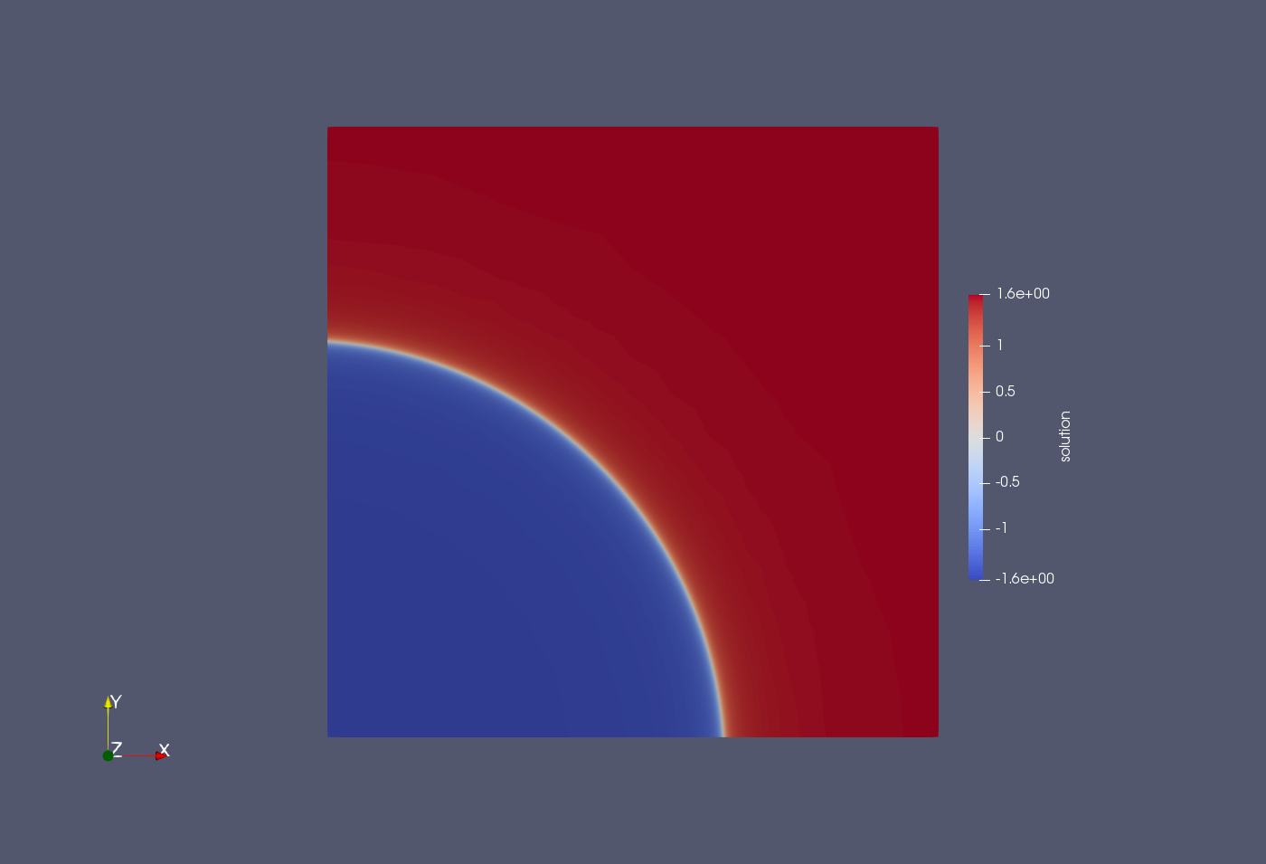
(a) 2D benchmark problem.

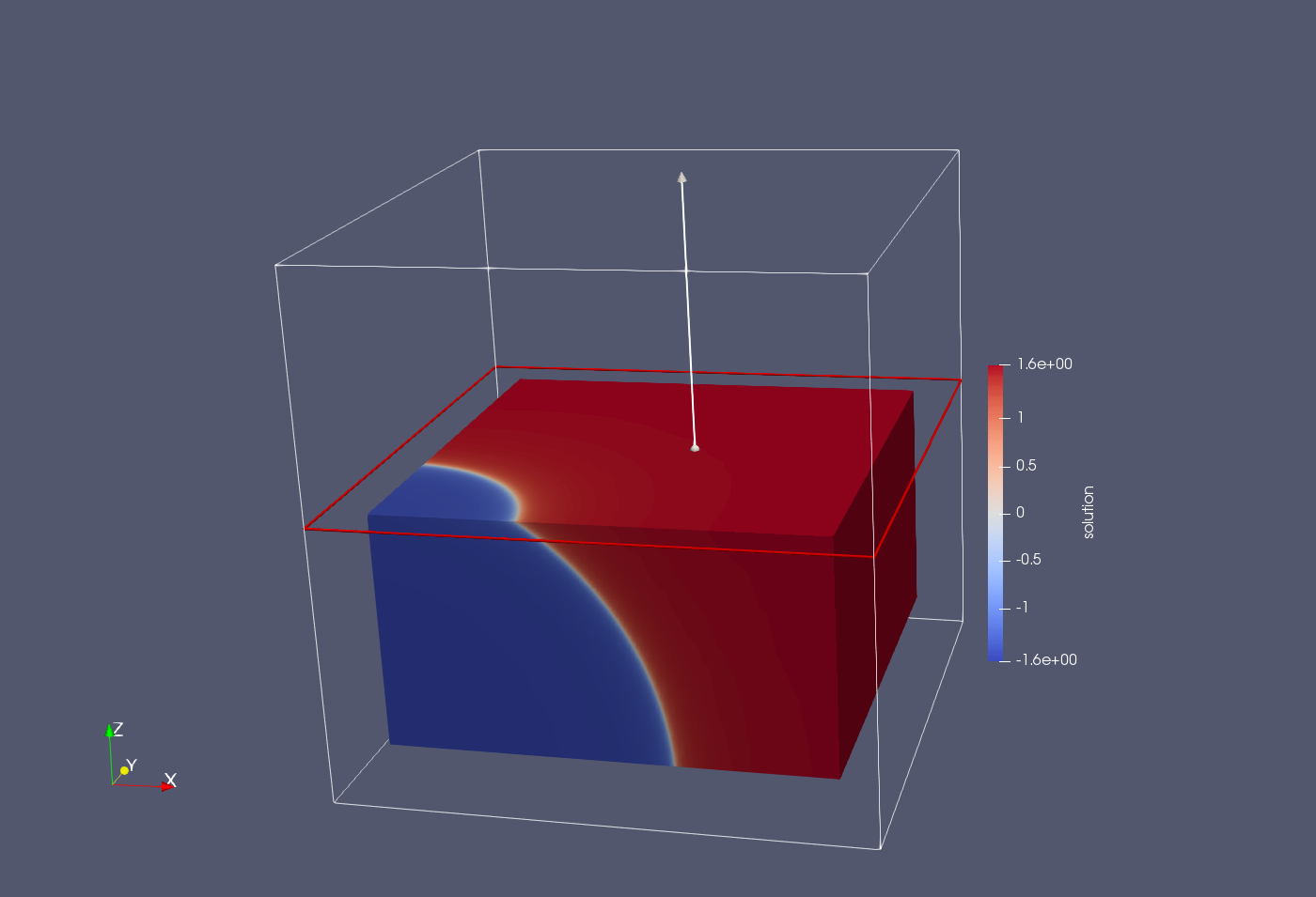
(b) 3D benchmark problem.

Figure 1. Manufactured solution (9) for Prob. (8).

5.2. FE discretization

Tutorial_01 implements two different FE formulations for the Poisson problem. On the one hand, a conforming Continuous Galerkin (CG) formulation, which is covered in Sect. 5.2.1, and a non-conforming DG one, covered in Sect. 5.2.2. In this tutorial, both formulations are used in combination with a uniform (thus conforming) triangulation $\mathcal{T}_{h}$ of $\Omega$ made of quadrilateral/hexahedral cells. Apart from solving (8), tutorial_01 also evaluates the FE discretization error. In particular, for each cell $K$, it computes the square of the error energy norm, which for the Poisson problem is defined as $e_{K}^{2}:=\int_{K}\operatorname{\boldsymbol{\nabla}}(u-u_{h})\cdot\operatorname{\boldsymbol{\nabla}}(u-u_{h})$, with $u$ and $u_{h}$ being the exact and FE solution, resp. It also records and prints on screen the total error $e:=(\sum_{K}e_{K}^{2})^{1/2}$. On user-demand, the cell quantities $e_{K}^{2}$ can be written to post-processing data files for later visualization; see Sect. 5.3 for more details.

5.2.1. CG FE formulation

In order to derive a CG FE formulation, one starts with the weak form of the problem at hand, the Poisson problem in the case of tutorial_01. This problem can be stated as in (1) with ${a}(u,v):=\int_{\Omega}\operatorname{\boldsymbol{\nabla}}u\cdot\operatorname{\boldsymbol{\nabla}}v$ and $\ell(v):=\int_{\Omega}fv$. The weak form (1) is discretized by replacing $H_{0}^{1}(\Omega)$ by a finite-dimensional space $V_{h}$, without any kind of perturbation. As we aim at building a conforming FE formulation, i.e., $V_{h}\subset H_{0}^{1}(\Omega)$, we must ensure that the conformity requirements of $H_{0}^{1}(\Omega)$ are fulfilled. In particular, we must ensure that the functions in $V_{h}$ have continuous trace across cell interfaces. We refer to  [37, Sect. 3] for a detailed exposition of how $H_{0}^{1}(\Omega)$-conforming FE spaces can be built using the so-called Lagrangian (a.k.a. nodal) FEs. When such FE is combined with hexahedral cells, $V_{h}|_{K}:=\mathcal{Q}_{q}(K)$, i.e., the space of multivariate polynomials that are of degree less or equal to $q$ with respect to each variable in $(x_{1},\ldots,x_{d})\in K$. The system matrix can be computed as described in (4) with ${a}_{K}(u,v):=\int_{K}\operatorname{\boldsymbol{\nabla}}u\cdot\operatorname{\boldsymbol{\nabla}}v$, ${\ell}_{K}(v):=\int_{K}fv$ (assuming $f\in L^{2}(\Omega)$).

5.2.2. DG FE formulation

Tutorial_01 also implements a non-conforming DG formulation for the Poisson problem. In particular, an IP DG formulation described in [43]. This formulation, as any other non-conforming discretization method, extracts the discrete solution $u_{h}$ from a global FE space $V_{h}$ which does not conform to $H^{1}(\Omega)$, i.e., $V_{h}\not\subset H^{1}(\Omega)$. In particular, $V_{h}$ is composed of functions that are continuous within each cell, but discontinuous across cells, i.e., $V_{h}=\{u_{h}\in L_{2}(\Omega):u_{h}|_{K}\in\mathcal{Q}_{q}(K)\subset H^{1}(K),\ K\in\mathcal{T}_{h}\}$, with $\mathcal{Q}_{q}(K)$ as defined in Sect. 5.2.1. While this extremely simplifies the construction of $V_{h}$, as one does not have to take care of the inter-cell continuity constraints required for $H^{1}(\Omega)$-conformity (see  [37, Sect. 3] for more details), one cannot plug $V_{h}$ directly into (1), since the original bilinear form has no sense for a non-conforming FE space. Instead, one requires judiciously numerical perturbations of the continuous bilinear and linear forms in (1) in order to weakly enforce conformity.

In the IP DG FE formulation at hand, and in contrast to the one presented in Sect. 5.2.1 (that imposes essential Dirichlet BCs strongly) the condition $u=g$ on $\Omega$ is weakly imposed, as it is natural in this kind of formulations. If we denote $\mathcal{F}^{\Omega}_{h}$ and $\mathcal{F}^{\partial\Omega}_{h}$ as the set of interior and boundary facets of $\mathcal{T}_{h}$, resp., the discrete weak form of IP DG method implemented by tutorial_01 reads: find $u_{h}\in V_{h}$ such that

(10) $${a_{h}}(u_{h},v_{h})=\ell_{h}(v_{h}),\,\qquad\hbox{for any }v_{h}\in V_{h},$$

with

(11) $$\begin{split}&{a_{h}}(u_{h},v_{h})=\sum_{K\in\mathcal{T}_{h}}\int_{K}\operatorname{\boldsymbol{\nabla}}u_{h}\cdot\operatorname{\boldsymbol{\nabla}}v_{h}-\\ &\sum_{F\in\mathcal{F}^{\Omega}_{h}}\int_{F}[\![v_{h}]\!]\cdot\{\!\!\{\operatorname{\boldsymbol{\nabla}}u_{h}\}\!\!\}-\tau\sum_{F\in\mathcal{F}^{\Omega}_{h}}\int_{F}[\![u_{h}]\!]\cdot\{\!\!\{\operatorname{\boldsymbol{\nabla}}v_{h}\}\!\!\}+\sum_{F\in\mathcal{F}^{\Omega}_{h}}\gamma|F|^{-1}\int_{F}[\![u_{h}]\!]\cdot[\![v_{h}]\!]-\\ &\sum_{F\in\mathcal{F}^{\partial\Omega}_{h}}\int_{F}v_{h}\operatorname{\boldsymbol{\nabla}}{u_{h}}\cdot\boldsymbol{n}-\tau\sum_{F\in\mathcal{F}^{\partial\Omega}_{h}}\int_{F}u_{h}\operatorname{\boldsymbol{\nabla}}{v_{h}}\cdot\boldsymbol{n}+\sum_{F\in\mathcal{F}^{\partial\Omega}_{h}}\gamma|F|^{-1}\int_{F}u_{h}v_{h},\end{split}$$

and

(12) $$\begin{split}\ell_{h}(v_{h})=\sum_{K\in\mathcal{T}_{h}}\int_{K}fv_{h}-\tau\sum_{F\in\mathcal{F}^{\partial\Omega}_{h}}\int_{F}g\operatorname{\boldsymbol{\nabla}}{v_{h}}\cdot\boldsymbol{n}+\sum_{F\in\mathcal{F}^{\partial\Omega}_{h}}\gamma|F|^{-1}\int_{F}gv_{h}.\end{split}$$

In (11) and (12), $\tau$ is a fixed constant that characterizes the particular method at hand, $\gamma$ is a facet-wise positive constant referred to as penalty parameter, and $|F|$ denotes the surface of the facet; $\tau$ and $\gamma$ should be suitably chosen such that $a_{h}(\cdot,\cdot)$ is well-posed (stable and continuous) in the discrete setting, and the FE formulation enjoys optimal rates of convergence [43]. Finally, if we denote as $K^{+}$ and $K^{-}$ the two cells that share a given facet, then $\{\!\!\{w_{h}\}\!\!\}$ and $[\![w_{h}]\!]$ denote mean values and jumps of $w_{h}$ across cells facets:

(13) $$\{\!\!\{w_{h}\}\!\!\}=\frac{w_{h}^{+}+w_{h}^{-}}{2},\quad\quad[\![w_{h}]\!]=w_{h}^{+}\boldsymbol{n}^{+}+w_{h}^{-}\boldsymbol{n}^{-},$$

with $\boldsymbol{n}^{+}$, $\boldsymbol{n}^{-}$ being the facet outward unit normals, and $w_{h}^{+}$, $w_{h}^{-}$ the restrictions of $w_{h}$ to the facet, both from either the perspective of $K^{+}$ and $K^{-}$, resp.

The assembly of the cell integrals in (11) and (12) is performed as described in Sect. 5.2.1. With regard to the facet integrals, assuming that we are sitting on an interior facet $F\in\mathcal{F}^{\Omega}_{h}$, four facet-wise matrices, namely $\mathbf{A}^{F}_{K^{+}K^{+}}$, $\mathbf{A}^{F}_{K^{+}K^{-}}$, $\mathbf{A}^{F}_{K^{-}K^{+}}$, and $\mathbf{A}^{F}_{K^{-}K^{-}}$, are computed. The entries of, e.g., $\mathbf{A}^{F}_{K^{+}K^{-}}$, are defined as:

(14) $$\left(\mathbf{A}^{F}_{K^{+}K^{-}}\right)_{ab}=-\int_{F}[\![\phi^{b}_{K^{-}}]\!]\cdot\{\!\!\{\operatorname{\boldsymbol{\nabla}}\phi^{a}_{K^{+}}\}\!\!\}-\tau\int_{F}[\![\phi^{a}_{K^{+}}]\!]\cdot\{\!\!\{\operatorname{\boldsymbol{\nabla}}\phi^{b}_{K^{-}}\}\!\!\}+\gamma|F|^{-1}\int_{F}[\![\phi^{a}_{K^{+}}]\!]\cdot[\![\phi^{b}_{K^{-}}]\!],$$

for $a,b=1,\ldots,\mathrm{dim}(\mathcal{Q}_{q}(K))$. This matrix is assembled into $\mathbf{A}$ as $\mathbf{A}_{[a][b]}\mathrel{+}=(\mathbf{A}^{F}_{K^{+}K^{-}})_{ab}$.

5.3. The commented code

The main program unit of tutorial_01 is shown in Listing 5. Apart from fempar_names, it also uses three tutorial-specific support modules in Lines 3-5. The one used in Line 3 implements the data type instances declared in Line 16 and 17, the one in Line 4, the ones declared in Lines 12 and 13, and the one in Line 5, the data type instance declared in Line 20. The rest of data type instances declared in part 2) of the tutorial program (Lines 6-21) are implemented within FEMPAR. Tutorial_01’s main executable code spans Lines 22-36. As there is almost a one-to-one mapping among the data type instances and the helper procedures called by tutorial_01, we will introduce them in the sequel step-by-step along with code snippets of the corresponding helper procedures. The setup_parameter_handler and get_tutorial_cla_values helper procedures have been already introduced in Sect. 4. Tutorial_01 registers CLAs to select the values of $\alpha$, $r$, and $x_{c}$ (see Sect. 5.1), and the FE formulation to be used (see Sect. 5.2).

⬇

1program tutorial_01_poisson_sharp_circular_wave

2 use fempar_names

3 use tutorial_01_discrete_integration_names

4 use tutorial_01_functions_names

5 use tutorial_01_error_estimator_names

6 ... ! Declaration of tutorial_01_... parameter constants

7 type(serial_context_t) :: world_context

8 type(environment_t) :: environment

9 type(serial_triangulation_t) :: triangulation

10 type(serial_fe_space_t) :: fe_space

11 type(strong_boundary_conditions_t) :: strong_boundary_conditions

12 type(sharp_circular_wave_source_term_t) :: source_term

13 type(sharp_circular_wave_solution_t) :: exact_solution

14 type(fe_affine_operator_t) :: fe_affine_operator

15 type(fe_function_t) :: discrete_solution

16 type(cg_discrete_integration_t), target :: cg_discrete_integration

17 type(dg_discrete_integration_t), target :: dg_discrete_integration

18 type(direct_solver_t) :: direct_solver

19 type(output_handler_t) :: output_handler

20 type(poisson_error_estimator_t) :: error_estimator

21 ... ! Declaration of variables storing CLA values particular to tutorial_01_...

22 call fempar_init()

23 call setup_parameter_handler()

24 call get_tutorial_cla_values()

25 call setup_context_and_environment()

26 call setup_triangulation()

27 call setup_problem_functions()

28 call setup_strong_boundary_conditions()

29 call setup_fe_space()

30 call setup_discrete_solution()

31 call setup_and_assemble_fe_affine_operator()

32 call solve_system()

33 call compute_error()

34 call write_postprocess_data_files()

35 call free_all_objects()

36 call fempar_finalize()

37contains

38 ... ! Implementation of helper procedures

39end program tutorial_01_poisson_sharp_circular_wave

Listing 5: Tutorial_01 program unit.

The setup_context_and_environment helper procedure is shown in Listing 6. Any FEMPAR program requires to set up (at least) one context and one environment. In a nutshell, a context is a software abstraction for a group of parallel tasks (a.k.a. processes) and the communication layer that orchestrates their concurrent execution. There are several context implementations in FEMPAR, depending on the computing environment targeted by the program. As tutorial_01 is designed to work in serial computing environments, world_context is declared of type serial_context_t. This latter data type represents a degenerated case in which the group of tasks is just composed by a single task. On the other hand, the environment organizes the tasks of the context from which it is set up into subgroups of tasks, referred to as levels, and builds up additional communication mechanisms to communicate tasks belonging to different levels. As world_context represents a single-task group, we force the environment to handle just a single level, in turn composed of a single task. This is achieved using the parameter_handler%update(...) calls in Lines 3 and 4 of Listing 6, resp; see Sect. 4. The rationale behind the environment will become clearer in tutorial_03, which is designed to work in distributed-memory computing environments using Message Passing Interface (MPI) as the communication layer.

⬇

1subroutine setup_context_and_environment()

2 call world_context%create()

3 call parameter_handler%update(environment_num_levels_key, 1)

4 call parameter_handler%update(environment_num_tasks_x_level_key, [1])

5 call environment%create(world_context, parameter_handler%get_values())

6end subroutine setup_context_and_environment

Listing 6: The setup_context_and_environment procedure.

The triangulation $\mathcal{T}_{h}$ of $\Omega$ is set up in Listing 7. FEMPAR provides a data type hierarchy of triangulations rooted at the so-called triangulation_t abstract data type [37, Sect. 7]. In the most general case, triangulation_t represents a non-conforming mesh partitioned into a set of subdomains (i.e., distributed among a set of parallel tasks) that can be $h$-adapted and/or re-partitioned (i.e., re-distributed among the tasks) in the course of the simulation. Tutorial_01, however, uses a particular type extension of triangulation_t, of type serial_triangulation_t, which represents a conforming mesh centralized on a single task that remains static in the course of the simulation. For this triangulation type, the user may select to automatically generate a uniform mesh for simple domains (e.g., a unit cube), currently of brick (quadrilateral or hexahedral) cells, or, for more complex domains, import it from mesh data files, e.g., generated by the GiD unstructured mesh generator [38]. Listing 7 follows the first itinerary. In particular, in Line 3, it forces the serial_triangulation_t instance to be generated by a uniform mesh generator of brick cells, and in Lines 5-12, that $\Omega=[0,1]^{d}$ is the domain to be meshed, as required by our model problem. The rest of parameter values of this mesh generator, such as, e.g., the number of cells per space dimension, are not forced, so that the user may specify them as usual via the corresponding CLAs. The actual set up of the triangulation occurs in the call at Line 13.

⬇

1subroutine setup_triangulation()

2 integer(ip) :: num_dims

3 call parameter_handler%update(static_triang_generate_from_key, &

4 static_triang_generate_from_struct_hex_mesh_generator)

5 call parameter_handler%get(struct_hex_mesh_generator_num_dims_key, num_dims)

6 if ( num_dims == 2 ) then

7 call parameter_handler%update(struct_hex_mesh_generator_domain_limits_key, &

8 [0.0_rp,1.0_rp,0.0_rp,1.0_rp])

9 else

10 call parameter_handler%update(struct_hex_mesh_generator_domain_limits_key, &

11 [0.0_rp,1.0_rp,0.0_rp,1.0_rp,0.0,1.0_rp])

12 end if

13 call triangulation%create(environment, parameter_handler%get_values())

14end subroutine setup_triangulation

Listing 7: The setup_triangulation procedure.

Listing 8 sets up the exact_solution and source_term objects. These represent the exact (analytical) solution $u$ and source term $f$ of our problem. The program does not need to implement the Dirichlet function $g$, as it is equivalent to $u$ in our model problem. While we do not cover their implementation here, the reader is encouraged to inspect the tutorial_01_functions_names module. Essentially, this module implements a pair of program-specific data types extending the so-called scalar_function_t FEMPAR data type. This latter data type represents an scalar-valued function $h$, and provides interfaces for the evaluation of $h(\boldsymbol{x})$, $\operatorname{\boldsymbol{\nabla}}h(\boldsymbol{x})$, etc., with $\boldsymbol{x}\in{}\mkern 1.0mu\overline{\mkern-1.0mu\Omega}$, to be implemented by type extensions. In particular, tutorial_01 requires $u(\boldsymbol{x})$ and $\operatorname{\boldsymbol{\nabla}}u(\boldsymbol{x})$ for the imposition of Dirichlet BCs, and the evaluation of the energy norm, resp., and $f(\boldsymbol{x})$ for the evaluation of the source term.

⬇

1subroutine setup_problem_functions()

2 call source_term%create(triangulation%get_num_dims(),&

3 alpha,circle_radius,circle_center)

4 call exact_solution%create(triangulation%get_num_dims(),&

5 alpha,circle_radius,circle_center)

6end subroutine setup_problem_functions

Listing 8: The setup_problem_functions subroutine.

Listing 9 sets up the strong_boundary_conditions object. With this object one can define the regions of the domain boundary on which to impose strong BCs, along with the function to be imposed on each of these regions. It is required for the FE formulation in Sect. 5.2.1 as, in this method, Dirichlet BCs are imposed strongly. It is not required by the IP DG formulation, and thus not set up by Listing 9 for such formulation. The rationale behind Listing 9 is as follows. Any FEMPAR triangulation handles internally (and provides on client demand) a set identifier (i.e., an integer number) per each Vertex, Edge, and Face (VEF) of the mesh. On the other hand, it is assumed that the mesh generator from which the triangulation is imported classifies the boundary of the domain into geometrical regions, and that, when the mesh is generated, it assigns the same set identifier to all VEFs which belong to the same geometrical region. For example, for $d=2$, the uniform mesh generator classifies the domain into 9 regions, namely the four corners of the box, which are assigned identifiers $1,\ldots,4$, the four faces of the box, which are assigned identifiers $1,\ldots,8$ , and the interior of the box, which is assigned identifier 9. For $d=3$, we have 27 regions, i.e., 8 corners, 12 edges, 6 faces, and the interior of the domain. (At this point, the reader should be able to grasp where the numbers 8 and 26 in Listing 9 come from.) With the aforementioned in mind, Listing 9 sets up the strong_boundary_conditions instance conformally with how the VEFs of the triangulation laying on the boundary are flagged with set identifiers. In the loop spanning Lines 6-11, it defines a strong boundary condition to be imposed for each of the regions that span the boundary of the unit box domain, and the same function, i.e., exact_solution, to be imposed on all these regions, as required by the model problem of tutorial_01.

⬇

1subroutine setup_strong_boundary_conditions()

2 integer(ip) :: i, boundary_ids

3 if ( fe_formulation == "CG" ) then

4 boundary_ids = merge(8, 26, triangulation%get_num_dims() == 2)

5 call strong_boundary_conditions%create()

6 do i = 1, boundary_ids

7 call strong_boundary_conditions%insert_boundary_condition(boundary_id=i, &

8 field_id=1, &

9 cond_type=component_1, &

10 boundary_function=exact_solution)

11 end do

12 end if

13end subroutine setup_strong_boundary_conditions

Listing 9: The setup_strong_boundary_conditions subroutine.

In Listing 10, tutorial_01 sets up the fe_space instance, i.e., the computer representation of $V_{h}$. In Line 3, the subroutine forces fe_space to build a single-field FE space, and in Line 4, that it is built from the same local FE for all cells $K\in\mathcal{T}_{h}$. In particular, from a scalar-valued Lagrangian-type FE (Lines 5-6 and 7-8, resp.), as required by our model problem. The parameter value corresponding to the polynomial order of $V_{h}|_{K}$ is not forced, and thus can be selected from the CLI. Besides, Listing 10 also forces the construction of either a conforming or non-conforming $V_{h}$, depending on the FE formulation selected by the user (see Lines 10 and 15, resp.). The actual set up of fe_space occurs in Line 11 and 16 for the conforming and non-conforming variants of $V_{h}$, resp. In the latter case, fe_space does not require strong_boundary_conditions, as there are not BCs to be strongly enforced in this case. The call in these lines generates a global numbering of the DOFs in $V_{h}$, and (if it applies) identifies the DOFs sitting on the regions of the boundary of the domain which are subject to strong BCs (combining the data provided by the triangulation and strong_boundary_conditions). Finally, in Lines 19 and 21, Listing 10 activates the internal data structures that fe_space provides for the numerical evaluation of cell and facet integrals, resp. These are required later on to evaluate the discrete bilinear and linear forms of the FE formulations implemented by tutorial_01. We note that the call in Line 21 is only required for the IP DG formulation, as in the CG formulation there are not facet integrals to be evaluated.

⬇

1subroutine setup_fe_space()

2 type(string) :: fes_field_types(1), fes_ref_fe_types(1)

3 call parameter_handler%update(fes_num_fields_key,1)

4 call parameter_handler%update(fes_same_ref_fes_all_cells_key,.true.)

5 fes_field_types(1) = String(field_type_scalar)

6 call parameter_handler%update(fes_field_types_key,fes_field_types)

7 fes_ref_fe_types(1) = String(fe_type_lagrangian)

8 call parameter_handler%update(fes_ref_fe_types_key, fes_ref_fe_types )

9 if ( fe_formulation == "CG" ) then

10 call parameter_handler%update(fes_ref_fe_conformities_key, [.true.])

11 call fe_space%create( triangulation = triangulation, &

12 conditions = strong_boundary_conditions, &

13 parameters = parameter_handler%get_values() )

14 else if ( fe_formulation == "DG" ) then

15 call parameter_handler%update(fes_ref_fe_conformities_key, [.false.])

16 call fe_space%create( triangulation = triangulation, &

17 parameters = parameter_handler%get_values() )

18 end if

19 call fe_space%set_up_cell_integration()

20 if ( fe_formulation == "DG" ) then

21 call fe_space%set_up_facet_integration()

22 end if

23end subroutine setup_fe_space

Listing 10: The setup_fe_space subroutine.

Listing 11 sets up the discrete_solution object, of type fe_function_t. This FEMPAR data type represents an element of $V_{h}$, the FE solution $u_{h}$ in the case of tutorial_01. In Line 2, this subroutine allocates room for storing the DOF values of $u_{h}$, and in Line 4, it computes the values of those DOFs of $u_{h}$ which lay on a region of the domain boundary which is subject to strong BCs, the whole boundary of the domain in the case of tutorial_01. The interpolate_dirichlet_values TBP of fe_space interpolates exact_solution, i.e., $u$, which is extracted from strong_boundary_conditions, using a suitable FE interpolator for the FE space at hand, i.e., the Lagrangian interpolator in the case of tutorial_01. FEMPAR supports interpolators for curl- and div-conforming FE spaces as well. Interpolation in such FE spaces involves the numerical evaluation of the functionals (moments) associated to the DOFs of $V_{h}$ [22].

⬇

1subroutine setup_discrete_solution()

2 call discrete_solution%create(fe_space)

3 if ( fe_formulation == "CG" ) then

4 call fe_space%interpolate_dirichlet_values(discrete_solution)

5 end if

6end subroutine setup_discrete_solution

Listing 11: The setup_discrete_solution subroutine.

In Listing 12, the tutorial program builds the fe_affine_operator instance, i.e., the computer representation of the operator defined in (3). Building this instance is a two-step process. First, we have to call the create TBP (see Line 12). Apart from specifying the data storage format and properties of the stiffness matrix $\mathbf{A}$, this call equips fe_affine_operator_t with all that it requires in order to evaluate the entries of the operator. Second, we have to call the compute TBP (Line 18), that triggers the actual numerical evaluation and assembly of the discrete weak form. With extensibility and flexibility in mind, this latter responsibility does not fall on fe_affine_operator_t, but actually on the data type extensions of a key abstract class defined within FEMPAR, referred to as discrete_integration_t [37, Sect. 11.2]. Tutorial_01 implements two type extensions of discrete_integration_t, namely cg_discrete_integration_t, and dg_..._t. The former implements (the discrete variant of) (1), while the second, (10). In Lines 3-11, Listing 12 passes to these instances the source term and boundary function to be imposed on the Dirichlet boundary. We note that the IP DG formulation works directly with the analytical expression of the boundary function (i.e., exact_solution), while the CG formulation with its interpolation (i.e., discrete_solution). Recall that the CG formulation imposes Dirichlet BCs strongly. In the approach followed by FEMPAR, the strong imposition of BCs requires the values of the DOFs of $u_{h}(=g_{h})$ sitting on the Dirichlet boundary when assembling the contribution of the cells that touch the Dirichlet boundary; see [37, 10.4]. On the other hand, the IP DG formulation needs to evaluate the last two facet integrals in (12) with the boundary function $g$ (i.e., $u$ in our case) as integrand. It is preferable that this formulation works with the analytical expression of the function, instead of its FE interpolation, to avoid an extra source of approximation error.

⬇

1subroutine setup_and_assemble_fe_affine_operator()

2 class(discrete_integration_t), pointer :: discrete_integration

3 if ( fe_formulation == "CG" ) then

4 call cg_discrete_integration%set_source_term(source_term)

5 call cg_discrete_integration%set_boundary_function(discrete_solution)

6 discrete_integration => cg_discrete_integration

7 else if ( fe_formulation == "DG" ) then

8 call dg_discrete_integration%set_source_term(source_term)

9 call dg_discrete_integration%set_boundary_function(exact_solution)

10 discrete_integration => dg_discrete_integration

11 end if

12 call fe_affine_operator%create ( sparse_matrix_storage_format = csr_format, &

13 diagonal_blocks_symmetric_storage = [ .true. ], &

14 diagonal_blocks_symmetric = [ .true. ], &

15 diagonal_blocks_sign = [ SPARSE_MATRIX_SIGN_POSITIVE_DEFINITE ], &

16 fe_space = fe_space, &

17 discrete_integration = discrete_integration )

18 call fe_affine_operator%compute()

19end subroutine setup_and_assemble_fe_affine_operator

Listing 12: The setup_and_assemble_fe_affine_operator subroutine.

Listing 13 finds the root of the FE operator, i.e., $u_{h}\in V_{h}$ such that $\mathcal{F}_{h}(u_{h})=0$. For such purpose, it first sets up the direct_solver instance (Lines 3-5) and later uses its solve TBP (Line 7). This latter method is fed with the “translation” of $\mathcal{F}_{h}$, i.e., the right hand side $\mathbf{f}$ of the linear system, and the free DOF values of $u_{h}$ as the unknown to be found. The free DOFs of $u_{h}$ are those whose values are not constrained, e.g., by strong BCs. direct_solver_t is a FEMPAR data type that offers interfaces to (non-distributed) sparse direct solvers provided by external libraries. In its first public release, FEMPAR provides interfaces to PARDISO [44] (the version available in the Intel MKL library) and UMFPACK [45], although it is designed such that additional sparse direct solver implementations can be easily added. We note that Listing 13 does not force any parameter value related to direct_solver_t; the default CLA values are appropriate for the Poisson problem. In any case, at this point the reader is encouraged to inspect the CLAs linked to direct_solver_t and play around them.

⬇

1subroutine solve_system()

2 class(vector_t), pointer :: dof_values

3 call direct_solver%set_type_from_pl(parameter_handler%get_values())

4 call direct_solver%set_parameters_from_pl(parameter_handler%get_values())

5 call direct_solver%set_matrix(fe_affine_operator%get_matrix())

6 dof_values => discrete_solution%get_free_dof_values()

7 call direct_solver%solve(fe_affine_operator%get_translation(),dof_values)

8end subroutine solve_system

Listing 13: The solve_system subroutine.

As any other FE program, tutorial_01 post-processes the computed FE solution. In particular, in the compute_error subroutine (Listing 14), it computes $e_{K}^{2}$ for each $K\in\mathcal{T}_{h}$, and the global error $e$; see Sect. 5.2. These quantities along with the FE solution $u_{h}$ are written to output data files for later visualization in the write_postprocess_data_files helper subroutine (Listing 15). The first subroutine relies on the error_estimator instance, implemented in one of the support modules of tutorial_01. In particular, the actual computation of $e_{K}^{2}$ occurs at the call to the compute_local_true_errors TBP of this data type (Line 6 of Listing 14). At this point, the user is encouraged to inspect the implementation of this data type in order to grasp how the numerical evaluation of the integrals required for the computation of $e_{K}^{2}$ is carried out using FEMPAR; see also [37, Sect. 8, 10.5].

⬇

1subroutine compute_error()

2 real(rp) :: global_error_energy_norm

3 call error_estimator%create(fe_space,parameter_handler%get_values())

4 call error_estimator%set_exact_solution(exact_solution)

5 call error_estimator%set_discrete_solution(discrete_solution)

6 call error_estimator%compute_local_true_errors()

7 global_error_energy_norm = &

8 sqrt(sum(error_estimator%get_sq_local_true_error_entries()))

9 ... ! Write error on screen along with the number of cells and DOFs

10end subroutine compute_error

Listing 14: The compute_error subroutine.

⬇

1subroutine write_postprocess_data_files()

2 if ( write_postprocess_data ) then

3 call output_handler%create(parameter_handler%get_values())

4 call output_handler%attach_fe_space(fe_space)

5 call output_handler%add_fe_function(discrete_solution, 1, ’solution’)

6 call output_handler%add_cell_vector(&

7 error_estimator%get_sq_local_true_errors(),&

8 ’cell_error_energy_norm_squared’)

9 call output_handler%open()

10 call output_handler%write()

11 call output_handler%close()

12 end if

13end subroutine write_postprocess_data_files

Listing 15: The write_postprocess_data_files subroutine.

The generation of output data files in Listing 15 is in charge of the output_handler instance. This instance lets the user to register an arbitrary number of FE functions (together with the corresponding FE space these functions were generated from) and cell data arrays (e.g., material properties or error estimator indicators), to be output in the appropriate format for later visualization. The user may also select to apply a differential operator to the FE function, such as divergence, gradient or curl, which involve further calculations to be performed on each cell. The first public release of FEMPAR supports two different data output formats, the standard-open model VTK [46], and the XDMF+HDF5 [47] model. The first format is the recommended option for serial computations (or parallel computations on a moderate number of tasks). The second model is designed with the parallel I/O data challenge in mind. It is therefore the recommended option for large-scale simulations in high-end computing environments. The data format to be used relies on parameter values passed to output_handler. As Listing 15 does not force any parameter value related to output_handler_t, tutorial_01 users may select the output data format readily from the CLI. At this point, the reader may inspect the CLAs linked to output_handler_t and play around them to see the differences in the output data files generated by Listing 15.

5.3.1. Discrete integration for a conforming method

As commented in Sect. 2 and one can observe in Listing 12, the definition of the FE operator requires a method that conceptually traverses all the cells in the triangulation, computes the element matrix and right-hand side at every cell, and assembles it in a global array. The abstract type in charge of this is the discrete_integration_t, which must be extended by the user to integrate their PDE system. In Listing 16, we consider a concrete version of this type for the Poisson equation using conforming Lagrangian FEs.

⬇

1subroutine cg_discrete_integration_integrate_galerkin (this, fe_space, assembler)

2 implicit none

3 class(cg_discrete_integration_t), intent(in) :: this

4 class(serial_fe_space_t) , intent(inout) :: fe_space

5 class(assembler_t) , intent(inout) :: assembler

6 class(fe_cell_iterator_t), allocatable :: fe

7 type(quadrature_t) , pointer :: quad

8 type(point_t) , pointer :: quad_coords(:)

9 type(vector_field_t) , allocatable :: shape_gradients(:,:)

10 real(rp) , allocatable :: shape_values(:,:)

11 real(rp), allocatable :: elmat(:,:), elvec(:)

12 integer(ip) :: qpoint, idof, jdof

13 real(rp) :: dV, source_term_value

14

15 call fe_space%create_fe_cell_iterator(fe)

16 ... ! Allocate elmat, elvec

17 do while ( .not. fe%has_finished() )

18 ! Update cell-integration related data structures

19 call fe%update_integration()

20 ! Get quadrature and quadrature coordinates mapped to physical space

21 quad => fe%get_quadrature()

22 quad_coords => fe%get_quadrature_points_coordinates()

23 ! Compute cell matrix and vector

24 elmat = 0.0_rp; elvec = 0.0_rp

25 call fe%get_values(shape_values)

26 call fe%get_gradients(shape_gradients)

27 do qpoint = 1, quad%get_num_quadrature_points()

28 dV = fe%get_det_jacobian(qpoint) * quad%get_weight(qpoint)

29 ! Compute cell matrix (bilinear form)

30 do idof = 1, fe%get_num_dofs()

31 do jdof = 1, fe%get_num_dofs()

32 elmat(idof,jdof) = elmat(idof,jdof) + &

33 dV * shape_gradients(jdof,qpoint) * shape_gradients(idof,qpoint)

34 end do

35 end do

36 ! Compute cell vector (linear form)

37 call this%source_term%get_value(quad_coords(qpoint),source_term_value)

38 do idof = 1, fe%get_num_dofs()

39 elvec(idof) = elvec(idof) + &

40 dV * source_term_value * shape_values(idof,qpoint)

41 end do

42 end do

43 ! Assemble elmat/elvec into assembler while taking care of strong

44 ! Dirichlet BCs (in turn extracted from this%discrete_boundary_function)

45 call fe%assembly( this%discrete_boundary_function, elmat, elvec, assembler )

46 call fe%next()

47 end do

48 call fe_space%free_fe_cell_iterator(fe)

49 ... ! Free shape_* arrays, elmat, elvec

50end subroutine cg_discrete_integration_integrate_galerkin

Listing 16: The integrate_galerkin TBP of the tutorial_01-specific cg_discrete_integration_t data type..

The integration of the (bi)linear forms requires cell integration machinery, which is provided by fe_space_t through the creation of the fe_cell_iterator_t in Line 15. Conceptually, the computed cell iterator is an object that provides mechanisms to iterate over all the cells of the triangulation (see Line 17 and Line 46). Positioned in a cell, it provides a set of cell-wise queries. All the integration machinery of a new cell is computed in Line 19. After this update of integration data, one can extract from the iterator the number of local shape functions (see Line 30) and an array with their values (resp., gradients) at the integration points in Line 25 (resp., Line 26). We note that the data types of the entries of these arrays can be scalars (see Line 10), vectors (of type vector_field_t, see Line 9), or tensors (of type tensor_field_t). It can also return information about the Jacobian of the geometrical transformation (see, e.g., the query that provides the determinant of the Jacobian of the cell map in Line 28). The iterator also provides a method to fetch the cell quadrature (see Line 21), which in turn has procedures to get the number of integration points (Line 27) and their associated weights (Line 28).

With all these ingredients, the implementation of the (bi)linear forms is close to its blackboard expression, making it compact, simple, and intuitive (see Line 32). It is achieved using operator overloading for different vector and tensor operations, e.g., the contraction and scaling operations (see, e.g., the inner product of vectors in Line 33). The computation of the right-hand side is similar. The only peculiarity is the consumption of the expression for $f$ in Line 37, which has to receive the quadrature points coordinates in physical space, i.e., with the entries of the quad_coords(:) array. We recall that cg_discrete_integration was supplied with the expression for $f$ in Listing 12.

The fe_cell_iterator_t data type also offers methods to assemble the element matrix and vector into assembler, which is the object that ultimately holds the global system matrix and right-hand side within the FE affine operator. The assembly is carried out in Line 45. The call in this line is provided with the DOF values of the function to be imposed strongly on the Dirichlet boundary, i.e., discrete_boundary_function; see discussion accompanying Listing 12 in Sect. 5.3.

5.3.2. Discrete integration for a non-conforming method

Let us consider the numerical integration of the IP DG method in (11). For non-conforming FE spaces, the formulation requires also a loop over the facets to integrate the perturbation DG terms. It can be written in a similar fashion to Sect. 5.3.1, but considering also facet-wise structures. For such purposes, FEMPAR provides FE facet iterators (see Line 19), which are similar to the FE cell iterators but traversing all the facets in the triangulation. This iterator provides a method to distinguish between boundary facets and interior facets (see Line 22), since different terms have to be integrated in each case. As above, at every facet, one can compute all the required numerical integration tools (see Line 24). After this step, one can also extract a facet quadrature (Line 25), which provides the number of quadrature points (see Line 27) and its weights (see Line 30). The FE facet iterator also provides methods that return $\boldsymbol{n}^{+}$, $\boldsymbol{n}^{-}$ (facet outward unit normals) (see Line 28), a characteristic facet size (see Line 29), or the determinant of the Jacobian of the geometrical transformation of the facet from the reference to the physical space (see Line 30).

An interior facet is shared between two and only two cells. After some algebraic manipulation, the DG terms in (11) can be decomposed into a set of terms that involve test functions (and gradients) of both cells, as shown in (14). The loop over the four facet matrices is performed in Lines 31-34. For each cell sharing the facet, one can also compute the shape functions and its gradients (see Lines 32-33 and 35-36). With all these ingredients, we compute the facet matrices in Lines 40-44. We note that the constant $\gamma$ in (11) has been defined in Line 18 as $10p^{2}$, where $p$ is the order of the FE space. The FE facet iterator also provides a method for the assembly of the facet matrices into global structures (see Line 50).

⬇

1subroutine dg_discrete_integration_integrate_galerkin (this, fe_space, assembler)

2 implicit none

3 class(dg_discrete_integration_t), intent(in) :: this

4 class(serial_fe_space_t) , intent(inout) :: fe_space

5 class(assembler_t) , intent(inout) :: assembler

6 ... ! Declare local variables in Listing 16

7 class(fe_facet_iterator_t), allocatable :: fe_face

8 real(rp), allocatable :: shape_values_Kminus(:,:), &

9 shape_values_Kplus(:,:)

10 type(vector_field_t), allocatable :: shape_gradients_Kminus(:,:), &

11 shape_gradients_Kplus(:,:)

12 type(vector_field_t) :: normals(2)

13 real(rp) :: h_length, C_IP ! Interior Penalty constant

14 real(rp), allocatable :: facemat(:,:,:,:), facevec(:,:)

15 integer(ip) :: Kminus, Kplus

16

17 ... ! Integrate and assemble cell integrals (see Listing 16)

18 C_IP = 10.0_rp * real(fe%get_order()**2, rp)

19 call fe_space%create_fe_facet_iterator(fe_face)

20 ... ! Allocate facemat, facevec

21 do while ( .not. fe_face%has_finished() ) ! Loop over all triangulation facets

22 if ( .not. fe_face%is_at_boundary() ) then ! Interior facet

23 ! Update facet-integration related data structures

24 call fe_face%update_integration()

25 quad => fe_face%get_quadrature() ! Get facet quadrature

26 facemat = 0.0_rp

27 do qpoint = 1, quad%get_num_quadrature_points()

28 call fe_face%get_normal(qpoint,normals)

29 h_length = fe_face%compute_characteristic_length(qpoint)

30 dV = fe_face%get_det_jacobian(qpoint) * quad%get_weight(qpoint)

31 do Kminus = 1, fe_face%get_num_cells_around()

32 call fe_face%get_values(Kminus,shape_values_Kminus)

33 call fe_face%get_gradients(Kminus,shape_gradients_Kminus)

34 do Kplus = 1, fe_face%get_num_cells_around()

35 call fe_face%get_values(Kplus,shape_values_Kplus)

36 call fe_face%get_gradients(Kplus,shape_gradients_Kplus)

37 do idof = 1, fe_face%get_num_dofs(Kminus)

38 do jdof = 1, fe_face%get_num_dofs(Kplus)

39 !- ({{grad u}}[[v]] + (1-xi)*[[u]]{{grad v}}) + C*p^2/h * [[u]] [[v]]

40 facemat(idof,jdof,Kminus,Kplus) = facemat(idof,jdof,Kminus,Kplus) + &

41 dV * &

42 (-0.5_rp*shape_gradients_Kplus(jdof,qpoint)*normals(Kminus)*shape_values_Kminus(idof,qpoint) - &

43 0.5_rp*shape_gradients_Kminus(idof,qpoint)*normals(Kplus)*shape_values_Kplus(jdof,qpoint) + &

44 c_IP / h_length * shape_values_Kplus(jdof,qpoint)*shape_values_Kminus(idof,qpoint)*normals(Kminus)*normals(Kplus))

45 end do

46 end do

47 end do

48 end do

49 end do

50 call fe_face%assembly( facemat, assembler )

51 else if ( fe_face%is_at_boundary() ) then

52 ... ! Integrate and assemble boundary facet terms

53 end if

54 call fe_face%next()

55 end do

56 call fe_space%free_fe_facet_iterator(fe_face)

57 ... ! Free shape_* arrays, facemat, facevec

58end subroutine dg_discrete_integration_integrate_galerkin

Listing 17: The integrate_galerkin TBP of the tutorial_01-specific dg_discrete_integration_t data type..

6. Tutorial_02: tutorial_01 problem tackled with AMR

6.1. Model problem

See Sect. 5.1.

6.2. FE discretization

While tutorial_01 uses a uniform (thus conforming) mesh $\mathcal{T}_{h}$ of $\Omega$, tutorial_02 combines the two FE formulations presented in Sect. 5.2 with a more clever/efficient domain discretization approach. Given that the solution of Prob. (8) exhibits highly localized features, in particular an internal sharp circular/spherical wave front layer, tutorial_02 exploits a FEMPAR triangulation data structure that efficiently supports dynamic $h$-adaptivity techniques (a.k.a. Adaptive Mesh Refinement and coarsening (AMR)), i.e., the ability of the mesh to be refined in the course of the simulation in those regions of the domain that present a complex behaviour (e.g., the internal layer in the case of Prob. (8)), and to be coarsened in those areas where essentially nothing relevant happens (e.g., those areas away from the internal layer). Tutorial_02 restricts itself to $h$-adaptivity techniques with a fixed polynomial order. This is in contrast to $hp$-adaptivity techniques, in which the local FE space polynomial order $p$ also varies among cells. In its first public release, the support of $hp$-adaptivity techniques in FEMPAR is restricted to non-conforming FE formulations.

In order to support AMR techniques, FEMPAR relies on the so-called forest-of-trees approach for efficient mesh generation and adaptation. Forest-of-trees can be seen as a two-level decomposition of $\Omega$, referred to as macro and micro level, resp. In the macro level, we have the so-called coarse mesh, i.e., a conforming partition $\mathcal{C}_{h}$ of $\Omega$ into cells $K\in\mathcal{C}_{h}$. For efficiency reasons, $\mathcal{C}_{h}$ should be as coarse as possible, but it should also keep the geometrical discretization error within tolerable margins. For complex domains, $\mathcal{C}_{h}$ is usually generated by an unstructured mesh generator, and then imported into the program. For simple domains, such as boxes in the case of Prob. (8), a single coarse cell is sufficient to resolve the geometry of $\Omega$. On the other hand, in the micro level, each of the cells of $\mathcal{C}_{h}$ becomes the root of an adaptive tree that can be subdivided arbitrarily (i.e., recursively refined) into finer cells. The locally refined mesh $\mathcal{T}_{h}$ to be used for FE discretization is defined as the union of the leaves of all adaptive trees.

In the case of quadrilateral (2D) or hexahedral (3D) adaptive meshes, the recursive application of the standard isotropic 1:4 (2D) and 1:8 (3D) refinement rule to the coarse mesh cells (i.e., to the adaptive tree roots) leads to adaptive trees that are referred to as quadtrees and octrees, resp., and the data structure resulting from patching them together is called forest-of-quadtrees and -octrees, resp., although the latter term is typically employed in either case. FEMPAR provides a triangulation data structure suitable for the construction of generic FE spaces $V_{h}$ (grad-, div-, and curl-conforming FE spaces) which exploits the p4est [1] library as its forest-of-octrees specialized meshing engine. We refer to [48, Sect. 3] for a detailed exposition of the design criteria underlying the $h$-adaptive triangulation in FEMPAR, and the approach followed in order to reconstruct it from the light-weight, memory-efficient representation of the forest-of-octrees that p4est handles internally.

Tree-based meshes provide multi-resolution capability by local adaptation. The cells in $\mathcal{T}_{h}$ (i.e., the leaves of the adaptive trees) might be located at different refinement level. However, these meshes are (potentially) non-conforming, i.e., they contain the so-called hanging VEFs. These occur at the interface of neighboring cells with different refinement levels. Mesh non-conformity introduces additional complexity in the implementation of both conforming and non-conforming FE formulations. In the former case, DOFs sitting on hanging VEFs cannot have an arbitrary value, as this would result in $V_{h}$ violating the trace continuity requirements for conformity across interfaces shared by a coarse cell and its finer cell neighbours. In order to restore conformity, the space $V_{h}$ has to be supplied with suitably defined algebraic constraints that express the value of hanging DOFs (i.e., DOFs sitting on hanging VEFs) as linear combinations of true DOFs (i.e., DOFs sitting on regular VEFs); see [48, Sect. 4]. These constraints, in most approaches available in the literature, are either applied to the local cell matrix and vector right before assembling them into their global counterparts, or, alternatively, eliminated from the global linear system later on (i.e., after FE assembly). In particular, FEMPAR follows the first approach. Therefore, hanging DOFs are not associated to an equation/unknown in the global linear system; see [48, Sect. 5]. On the other hand, in the case of non-conforming FE formulations, the facet integration machinery has to support the evaluation of flux terms across neighbouring cells at different refinement levels, i.e., facet integrals on each of the finer subfacets hanging on a coarser facet. FEMPAR supports such kind of facet integrals as well.

Despite the aforementioned, we note the following. First, the degree of implementation complexity is significantly reduced by enforcing the so-called 2:1 balance constraint, i.e., adjacent cells may differ at most by a single level of refinement; the $h$-adaptive triangulation in FEMPAR always satisfies this constraint [48]. Second, the library is entirely responsible for handling such complexity. Library users are not aware of mesh non-conformity when evaluating and assembling the discrete weak form of the FE formulation at hand. Indeed, as will be seen in Sect. 6.3, tutorial_02 re-uses “as-is” the cg_discrete_integration_t, and dg_..._t objects of tutorial_01; see Sect. 5.3.

6.3. The commented code

In order to illustrate the AMR capabilities in FEMPAR, while generating a suitable mesh for Prob. (8), tutorial_01 performs an AMR loop comprising the steps shown in Fig. 2.

1. Generate a conforming mesh $\mathcal{T}_{h}$ by uniformly refining, a number user-defined steps, a single-cell coarse mesh $\mathcal{C}_{h}$ representing the unit box domain (i.e., $\Omega$ in Prob. (8)).

2. Compute an approximate FE solution $u_{h}$ using the current mesh $\mathcal{T}_{h}$.

3. Compute $e_{K}^{2}$ for all cells $K\in\mathcal{T}_{h}$; see Sect. 5.2.

4. Given user-defined refinement and coarsening fractions, denoted by $\alpha_{r}$ and $\alpha_{c}$, resp., find thresholds $\theta_{r}$ and $\theta_{c}$ such that the number of cells with $e_{K}>\theta_{r}$ (resp., $e_{K}<\theta_{c}$) is (approximately) a fraction $\alpha_{r}$ (resp., $\alpha_{c}$) of the number of cells in $\mathcal{T}_{h}$.

5. Refine and coarsen the mesh cells, i.e., generate a new mesh $\mathcal{T}_{h}$, accordingly to the input provided by the previous step.

6. Repeat steps (2)-(5) a number of user-defined steps.

Figure 2. Tutorial_02 AMR loop.

The main program unit of tutorial_02 is shown in Listing 18. Tutorial_02 re-uses “as-is” the tutorial-specific modules of tutorial_01: no adaptations of these modules are required despite the higher complexity underlying FE discretization on non-conforming meshes; see Sect. 6.2. Compared to tutorial_01, tutorial_02 declares the triangulation instance to be of type p4est_serial_triangulation_t (instead of serial_triangulation_t). This data type extension of triangulation_t supports dynamic $h$-adaptivity (see Sect. 6.2) on serial computing environments (i.e., the triangulation is not actually distributed, but centralized on a single task) using p4est under the hood. On the other hand, it declares the refinement_strategy instance, of type fixed_fraction_refinement_strategy_t. The role of this FEMPAR data type in the loop of Fig. 2 will be clarified along the section.

⬇

1program tutorial_02_poisson_sharp_circular_wave_amr

2 use fempar_names

3 ... ! Use tutorial_01_... support modules

4 implicit none

5 ... ! Declaration of tutorial_02_... parameter constants

6 type(p4est_serial_triangulation_t) :: triangulation

7 type(fixed_fraction_refinement_strategy_t) :: refinement_strategy

8 ... ! Declaration of remaining objects of tutorial_02_... (see Listing 5)

9 ... ! Declaration of variables storing tutorial_02_... CLA values

10 call fempar_init()

11 call setup_parameter_handler()

12 call get_tutorial_cla_values()

13 call setup_context_and_environment()

14 current_amr_step = 0

15 ... ! See Lines 26-33 of Listing 18

16 call setup_refinement_strategy()

17 call output_handler_initialize()

18 do

19 call output_handler_write_current_amr_step()

20 if ( current_amr_step == num_amr_steps ) exit

21 current_amr_step = current_amr_step + 1

22 call refinement_strategy%update_refinement_flags(triangulation)

23 call setup_triangulation()

24 call setup_fe_space()

25 call setup_discrete_solution()

26 call setup_and_assemble_fe_affine_operator()

27 call solve_system()

28 call compute_error()

29 end do

30 call output_handler_finalize()

31 call free_all_objects()

32 call fempar_finalize()

33contains

34 ... ! Implementation of helper procedures

35end program tutorial_02_poisson_sharp_circular_wave_amr

Listing 18: Tutorial_02 program unit.

Tutorial_02’s main executable code spans Lines 10-32. Apart from those CLAs registered by tutorial_01, in the call to setup_parameter_handler, tutorial_02 registers two additional CLAs to specify the number of user-defined uniform refinement and AMR steps in Steps (1) and (6), resp., of Fig. 2. The main executable code of Tutorial_02 is mapped to the steps in Fig. 2 as follows. Line 15, which actually triggers a sequence of calls equivalent to Lines 26-33 of Listing 18, corresponds to Step (1), (2) and (3) with $\mathcal{T}_{h}$ being the initial conforming mesh generated by means of a user-defined number of uniform refinement steps. In particular, the call to setup_triangulation implements Step (1), and the call to compute_error, Step (3). The rest of calls within Lines 26-33 of Listing 18 are required to implement Step (2). The loop in Listing 18 spanning Lines 18-29, implements the successive generation of a sequence of hierarchically refined meshes. In particular, Line 22 implements Step (4) of Fig. 2, Line 23 Step (5), and Lines 24-27 and Line 28 Step (2) and Step (3), resp., with $\mathcal{T}_{h}$ being the newly generated mesh.

The tutorial_01 helper subroutines in Listings 6, 8, 9, and 11, are re-used “as-is” for tutorial_02. In the particular case of setup_strong_boundary_conditions, this is possible as the $h$-adaptive triangulation assigns the VEF set identifiers equivalently to the triangulation that was used by tutorial_01 (when both are configured to mesh box domains). The rest of tutorial_02 helper subroutines have to be implemented only slightly differently to the ones of tutorial_01. In particular, tutorial_02 handles the current_amr_step counter; see Listing 18. Right at the beginning, the counter is initialized to zero (see Line 14), and incremented at each iteration of the loop spanning Lines 18-29 (Line 21). Thus, this counter can be used by the helper subroutines to distinguish among two possible scenarios. If current_amr_step == 0, the program is located on the initialization section right before the loop, or within this loop otherwise. The usage of current_amr_step by setup_triangulation and setup_fe_space is illustrated in Listings 19 and 20, resp.

⬇

1subroutine setup_triangulation()

2 integer(ip) :: i, num_dims

3 if ( current_amr_step == 0 ) then

4 ... ! Force the triangulation to mesh the unit box domain

5 call triangulation%create(environment, parameter_handler%get_values())

6 do i=1, num_uniform_refinement_steps

7 call flag_all_cells_for_refinement()

8 call triangulation%refine_and_coarsen()

9 end do

10 else

11 call triangulation%refine_and_coarsen()

12 end if

13end subroutine setup_triangulation

14

15subroutine flag_all_cells_for_refinement()

16 class(cell_iterator_t), allocatable :: cell

17 call triangulation%create_cell_iterator(cell)

18 do while ( .not. cell%has_finished() )

19 call cell%set_for_refinement()

20 call cell%next()

21 end do

22 call triangulation%free_cell_iterator(cell)

23end subroutine flag_all_cells_for_refinement

Listing 19: The setup_triangulation procedure.

⬇

1subroutine setup_fe_space()

2 if ( current_amr_step == 0 ) then

3 ... ! See Listing  10

4 else

5 call fe_space%refine_and_coarsen()

6 end if

7end subroutine setup_fe_space

Listing 20: The setup_fe_space subroutine.

In Listing 19 one may readily observe that the setup_triangulation helper subroutine behaves differently depending on the value of current_amr_step. When its value is zero (Lines 4-9), the subroutine first generates a triangulation of the unit box domain which is composed of a single brick cell, i.e., a forest-of-octrees with a single adaptive octree (Lines 4 5). Then, it enters a loop in which the octree root is refined uniformly num_uniform_refinement_steps times (Lines 6-9) in order to generate $\mathcal{T}_{h}$ in Step (1) of Fig. 2; this program variable holds the value provided by the user through the corresponding CLA. The loop relies on the flag_all_cells_for_refinement helper procedure, which is shown in Lines 15-23 of Listing 19, and the refine_and_coarsen TBP of triangulation (Line 8). The first procedure walks through over the mesh cells, and for each cell, sets a per-cell flag that tells the triangulation to refine the cell, i.e., we flag all cells for refinement, in order to obtain a uniformly refined mesh. On the other hand, the refine_and_coarsen TBP adapts the triangulation based on the cell flags set by the user, while transferring data that the user might have attached to the mesh objects (e.g., cells and VEFs set identifiers) to the new mesh objects generated after mesh adaptation.

When current_amr_step is larger than zero, Listing 19 invokes the refine_and_coarsen TBP of the triangulation (Line 11). As commented in the previous paragraph, this procedure adapts the mesh accordingly to how the mesh cells have been marked for refinement, coarsening, or to be left as they were prior to adaptation. This latter responsibility falls on the refinement_strategy instance, and in particular in its update_refinement_flags TBP. This TBP, which is called in Line 22 of Listing 18, right before the call to setup_triangulation in Line 23 of Listing 18, follows the strategy in Step (4) of Fig. 2.

Listing 20 follows the same pattern as Listing 19. When the value of current_amr_step is zero, it sets up the fe_space instance using exactly the same sequence of calls as in Listing 10. When the value of current_amr_step is larger than zero, it calls the refine_and_coarsen TBP of fe_space to build a new global FE space $V_{h}$ from the newly generated triangulation, while trying to re-use its already allocated internal data buffers as much as possible. Optionally, this TBP can by supplied with a FE function $u_{h}$ (or, more generally, an arbitrary number of them). In such a case, refine_and_coarsen injects the FE function provided into the newly generated $V_{h}$ by using a suitable FE projector for the FE technology being used, the Lagrangian interpolator in the case of tutorial_02. This feature is required by numerical solvers of transient and/or non-linear PDEs.

Listing 21 shows those lines of code of the solve_system procedure of tutorial_02 which are different to its tutorial_01 counterpart in Listing 13. Apart from the fact that Listing 21 follows the same pattern as Listings 19 and 20, the reader should note the call to the update_hanging_dof_values TBP of fe_space in Line 9. This TBP computes the values of $u_{h}$ corresponding to hanging DOFs using the algebraic constraints required to enforce the conformity of $V_{h}$; see Sect. 6.2. This is required each time that the values of $u_{h}$ corresponding to true DOFs are updated (e.g., after linear system solution). Not calling it results in unpredictable errors during post-processing, or even worse, during a non-linear and/or time-stepping iterative solution loop, in which the true DOF values of $u_{h}$ are updated at each iteration.

⬇

1subroutine solve_system()

2 if ( current_amr_step == 0 ) then

3 ... ! Lines 3-5 of Listing 13

4 else

5 call direct_solver%reallocate_after_remesh()

6 end if

7 ... ! Lines 6-7 of Listing 13

8 if ( fe_formulation == "CG" ) then

9 call fe_space%update_hanging_dof_values(discrete_solution)

10 end if

11end subroutine solve_system

Listing 21: The solve_system subroutine.

Listing 22 shows the helper subroutine that sets up the refinement_strategy object. As mentioned above, this object implements the strategy in Step (2) of Fig. 2. In Lines 2-3, the procedure forces refinement_strategy to use parameter values $\alpha_{r}=0.1$ and $\alpha_{c}=0.05$; see Step (2) of Fig. 2. The actual set up of refinement_strategy occurs at Line 5. We note that, in this line, refinement_strategy is supplied with the error_estimator instance, of type poisson_error_estimator_t. This tutorial-specific data type, which is also used by tutorial_01, extends the error_estimator_t FEMPAR abstract data type. This latter data type is designed to be a place-holder of a pair of cell data arrays storing the per-cell true and estimated errors, resp. These arrays are computed by the data type extensions of error_estimator_t in the compute_local_true_errors and compute_local_estimates (deferred) TBPs. Neither tutorial_02 nor tutorial_01 actually uses a-posteriori error estimators. Thus, the compute_local_estimates TBP of poisson_error_estimator_t just copies the local true errors into the estimated errors array. While the compute_error helper subroutine of tutorial_01 (Listing 14) does not call the compute_local_estimates TBP, its counterpart in tutorial_02 must call it, as the refinement_strategy object extracts the data to work with from the error estimators array of error_estimator.

⬇

1subroutine setup_refinement_strategy()

2 call parameter_handler%update(ffrs_refinement_fraction_key, 0.10_rp)

3 call parameter_handler%update(ffrs_coarsening_fraction_key, 0.05_rp)

4 call parameter_handler%update(ffrs_max_num_mesh_iterations_key, num_amr_steps)

5 call refinement_strategy%create(error_estimator,parameter_handler%get_values())

6end subroutine setup_refinement_strategy

Listing 22: The setup_refinement_strategy subroutine.

Listing 18 handles the output of post-processing data files rather differently from Listing 5. It in particular generates simulation results for the full set of triangulations generated in the course of the simulation. In order to do so, it relies on the ability of output_handler_t to manage the time steps in transient simulations on a sequence of triangulations which might be different at each single time step. The output_..._initialize procedure resembles Listing 15, except that it does not call neither the write nor the close TBPs of output_handler_t. Besides, it forces a parameter value of output_handler_t to inform it that the triangulation might be different at each single step. If the mesh does not evolve dynamically, then it is only written once, instead of at every step, saving disk storage (as far as such feature is supported by the output data format). The output_handler_write_..._step procedure (see Listing 18) first calls the append_time_step and, then, the write TBPs of output_handler_t. The combination of these two calls outputs a new step into the output data files. Finally, the output_handler_finalize procedure (see Listing 18) just calls the close TBP of output_handler_t. This call closes all file units handled by output_handler, thus flushing into disk all pending write operations.

6.4. Numerical results

In Fig. 3(a) and 3(b) we show the FE solution computed by tutorial_02, along with $e_{K}^{2}$, for all $K\in\mathcal{T}_{h}$, for the 2D version of Problem (5.1) discretized with an adapted mesh resulting from 8 and 20 AMR steps, resp., and bilinear Lagrangian FEs. The number of initial uniform refinement steps was set to 2, resulting in an initial conforming triangulation made of 16 quadrilateral cells. As expected, the mesh tends to be locally refined close to the internal layer.

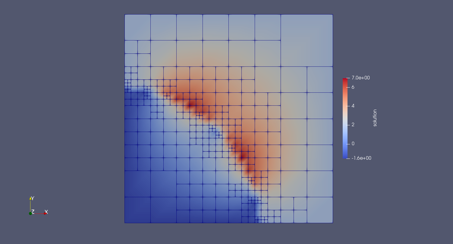
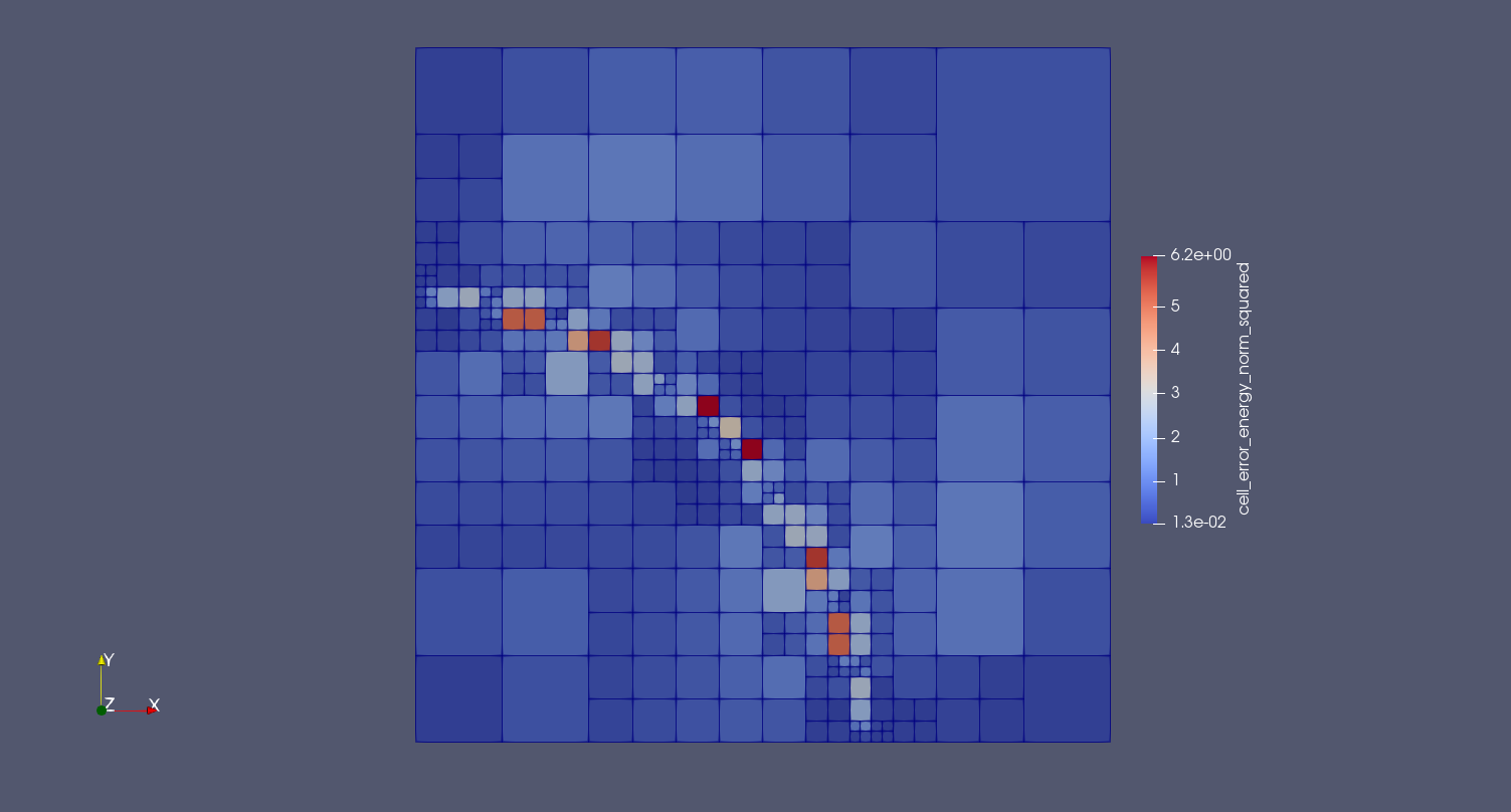
(a) 8 AMR steps; 322 cells; 243 (true) DOFs.

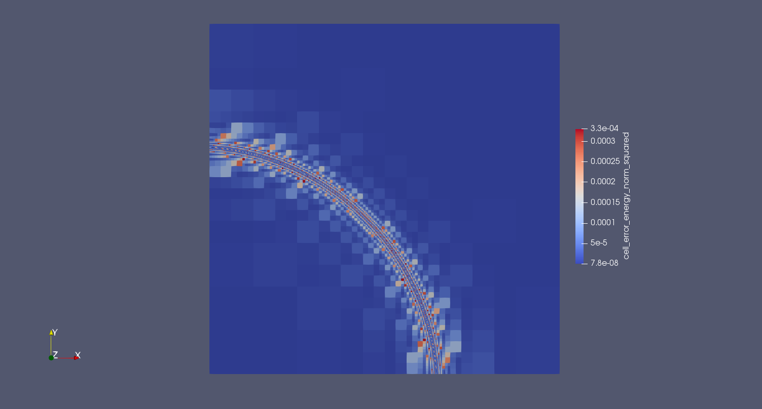
(b) 20 AMR steps; 13,564 cells; 11,535 (true) DOFs.

Figure 3. Mesh and FE solution (left) and $e_{K}^{2}$ for all $K\in\mathcal{T}_{h}$ (right).

On the other hand, in Fig. 4, we show error convergence history plots for the 2D benchmark problem. The results in Fig. 4(a) were obtained with tutorial_01, while those in Fig.4(b), with tutorial_02. As expected, the benefit of using local refinement is substantial for the problem at hand.

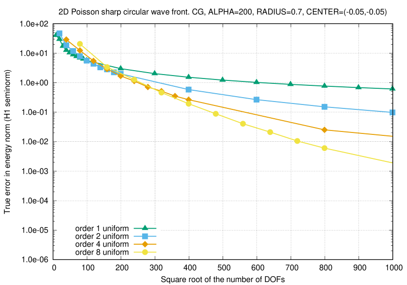
(a) Uniform meshing.

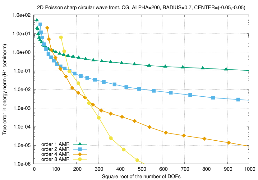
(b) AMR.

Figure 4. Convergence history for the 2D benchmark problem using the CG FE formulation with different polynomial order.

7. Tutorial_03: Distributed-memory parallelization of tutorial_02

7.1. Model problem

See Sect. 5.1.

7.2. Parallel FE discretization

Tutorial_03 exploits a set of fully-distributed data structures and associated algorithms available in FEMPAR for the scalable solution of PDE problems in high-end distributed-memory computers [48]. Such data structures are driven by tutorial_03 in order to efficiently parallelize the AMR loop of tutorial_02 (Fig. 2). In order to find $u_{h}$ at each adaptation step (Step (2), Fig. 2), tutorial_03 combines the CG FE formulation for Prob. (8) (Sect. 5.2.1) with a scalable domain decomposition preconditioner for the fast iterative solution of the linear system resulting from FE discretization. In this section, we briefly introduce some key ideas underlying the extension of the approach presented in Sect. 6.2 to distributed computing environments. On the other hand, Sect. 7.3 overviews the preconditioning approach used by tutorial_03, and its parallel implementation in FEMPAR.

It order to scale FE simulations to large core counts, the adaptive mesh must be partitioned (distributed) among the parallel tasks such that each of these only holds a local portion of the global mesh. (The same requirement applies to the rest of data structures in the FE simulation pipeline, i.e., FE space, linear system, solver, etc.) Besides, as the solution might exhibit highly localized features, dynamic mesh adaptation can result in an unacceptable amount of load imbalance. Thus, it urges that the adaptive mesh data structure supports dynamic load-balancing, i.e., that it can be re-distributed among the parallel processes in the course of the simulation. As mentioned in Sect. 6.2, dynamic $h$-adaptivity in FEMPAR relies on forest-of-trees meshes. Modern forest-of-trees manipulation engines provide a scalable, linear runtime solution to the mesh (re-)partitioning problem based on the exploitation of Space-Filling Curves. SFCs provide a natural means to assign an ordering of the forest-of-trees leaves, which is exploited for the parallel arrangement of data. For example, in the p4est library, the forest-of-octrees leaves are arranged in a global one-dimensional data array in increasing Morton index ordering [1]. This ordering corresponds geometrically with the traversal of a $z$-shaped SFC (a.k.a. Morton SFC) of $\mathcal{T}_{h}$; see Fig. 5(a). This approach allows for fast dynamic repartitioning. A partition of $\mathcal{T}_{h}$ is simply generated by dividing the leaves in the linear ordering induced by the SFC into as many equally-sized segments as parallel tasks involved in the computation.

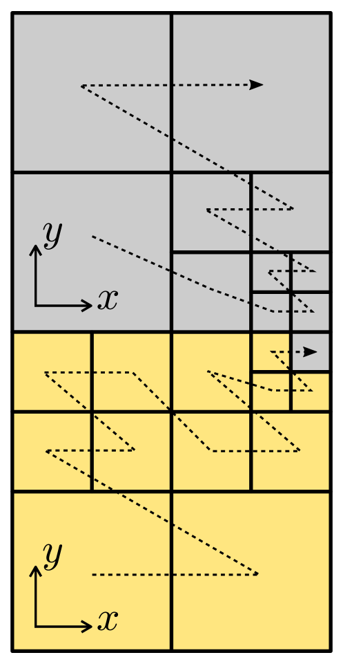
(a) $\mathcal{T}_{h}$.

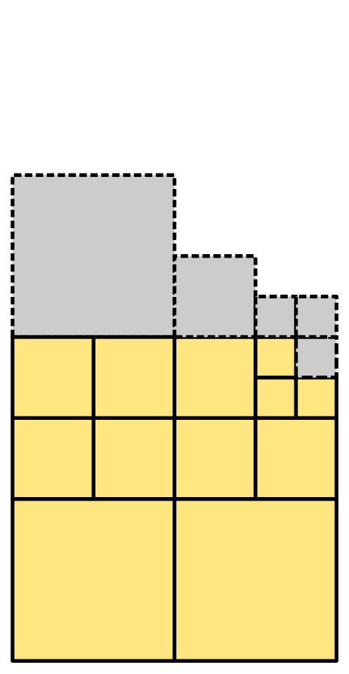
(b) $\mathcal{T}_{h}^{1}$.

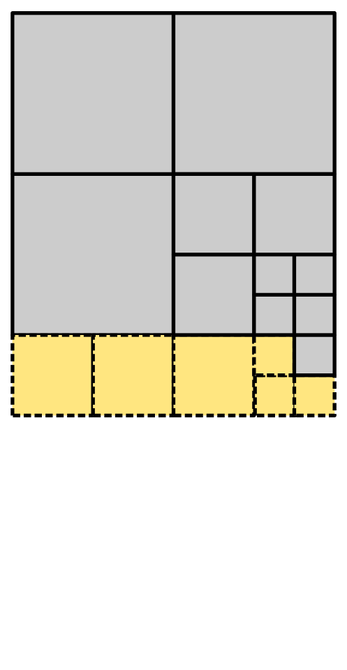
(c) $\mathcal{T}_{h}^{2}$.

Figure 5. 2:1 balanced forest-of-quadtrees mesh with two quadtrees (i.e., $|\mathcal{C}_{h}|=2$) distributed among two processors, 1:4 refinement and the Morton SFC [1]. Local cells are depicted with continuous boundary lines, while those in the ghost layer with dashed ones.

The parallel $h$-adaptive triangulation in FEMPAR reconstructs the local portion of $\mathcal{T}_{h}$ corresponding to each task from the distributed forest-of-octrees that p4est handles internally [48]. These local portions are illustrated in Fig. 5(b) and 5(c) when the forest-of-octrees in Fig 5(a) is distributed among two processors. The local portion of each task is composed by a set of cells that it owns, i.e., the local cells of the task, and a set of off-processor cells (owned by remote processors) which are in touch with its local cells, i.e., the ghost cells of the task. This overlapped mesh partition is used by the library to exchange data among nearest neighbours, and to glue together the global DOFs of $V_{h}$ which are sitting on the interface among subdomains, as required in order to construct FE spaces for conforming FE formulations in a distributed setting [48].

The user of the library, however, should also be aware to some extent of the distributed data layout of the triangulation. Depending on the numerical method at hand, it might be required to perform computations that involve the ghost cells, or to completely avoid them. For example, the computation of facet integrals on the interface among subdomains requires access to the ghost cells data (e.g., local shape functions values and gradients). On the other hand, cell integrals are typically assembled into global data structures distributed across processors (e.g., the linear system or the global energy norm of the error). While it is practically possible to evaluate a cell integral over a ghost cell in FEMPAR, this would result in excess computation, and even worse, to over-assembly due to the overlapped mesh partition (i.e., to wrong results). To this end, cell iterators of the parallel $h$-adaptive triangulation provide TBPs that let the user to distinguish among local and ghost cells, e.g., in an iteration over all cells of the mesh portion of a parallel task.

7.3. Fast and scalable parallel linear system solution

Tutorial_03 solves the linear system resulting from discretization iteratively via (preconditioned) Krylov subspace solvers [50]. To this end, FEMPAR provides abstract implementations (i.e., that can be leveraged either in serial or distributed computing environments, and/or for scalar or blocked layouts of the linear(ized) system) of a rich suite of solvers of this kind, such as, e.g., the Conjugate Gradients and GMRES solvers. Iterative solvers are much better suited than sparse direct solvers for the efficient exploitation of distributed-memory computers. However, they have to be equipped with an efficient preconditioner, a cornerstone ingredient for convergence acceleration, robustness and scalability.

Preconditioners based on the DD approach [51] are an appealing solution for the fast and scalable parallel iterative solution of linear systems arising from PDE discretization [52, 24, 53]. DD preconditioners make explicit use of the partition of the global mesh into sub-meshes (see Fig. 5), and involve the solution of local problems and communication among nearest-neighbour subdomains. In order to achieve algorithmic scalability, i.e., a condition number that remains constant as the problem size and number of subdomains are scaled, they have to be equipped with a suitably defined coarse-grid correction. The coarse-grid correction globally couples all subdomains and rapidly propagates the error correction information across the whole domain. However, it involves the solution of a global problem whose size typically increases (at best) linearly with respect to the number of subdomains. If not tackled appropriately by the underlying parallel implementation[52, 24, 53], this increase can jeopardize the practical scalability limits of this kind of preconditioners.

Among the set of scalable DD preconditioners available in the literature [51, 54], FEMPAR built-in preconditioning capabilities are grounded on the so-called BDDC preconditioning approach [55, 52], and its multi-level extension[56, 24] for extreme-scale computations. BDDC preconditioners belong to the family of non-overlapping DD methods [51]. Computationally speaking, BDDC preconditioners require to solve a local Dirichlet and a local constrained Neumann problem at each subdomain, and a global coarse-grid problem [55]. These methods rely on the definition of a FE space, referred to as the BDDC space, with relaxed inter-subdomain continuity. The local constrained Neumann problems and the global coarse-grid problem are required in order to extract a correction of the solution from the BDDC space. Such space is defined by choosing some quantities to be continuous across subdomain interfaces, i.e., the coarse or primal DOFs. The definition of the coarse DOFs in turn relies on a geometrical partition of the mesh VEFs laying on the subdomain interfaces into coarse objects, i.e., coarse VEFs. Next, we associate to some (or all) of these objects a coarse DOF. Once a correction has been extracted from the BDDC space, the continuity of the solution at the interface between subdomains is restored with an averaging operator.

The actual definition of the coarse DOFs depends on the kind of FE space being used for PDE discretization. For grad-conforming (i.e., $H^{1}$-conforming) FE spaces, as those required for the discretization of the Poisson PDE, the coarse DOFs of a FE function $u_{h}$ are defined as the value of the function at vertices, or the mean values of the function on coarse edges/faces. These concepts have been generalized for div- and curl-conforming FE spaces as well; see, e.g., [35], and references therein, for the latter kind of spaces.

While tutorial_03 uses a 2-level BDDC preconditioner suitable for the Poisson PDE, FEMPAR actually goes much beyond than that by providing an abstract OO framework for the implementation of widely applicable BDDC-like preconditioners. It is not the aim of this paper that the reader fully understands the complex details underlying this framework. However, it is at least convenient to have some familiarity with the data types on which the framework relies, and their basic roles in the construction of a BDDC preconditioner, as these are exposed in the code of tutorial_03 in Sect. 7.4. These are the following ones:

• coarse_triangulation_t. The construction of this object starts with the usual FE discretization mesh distributed among parallel tasks; see Fig. 5. Each of these tasks locally classifies the mesh VEFs lying on the interface among its local and ghost cells into coarse VEFs (see discussion above). Then, these coarse VEFs are glued together across parallel tasks by generating a global numbering of coarse VEFs in parallel. Finally, all coarse cells (i.e., subdomains) and its coarse VEFs are transferred from each parallel task to an specialized task (or set of tasks in the case it is distributed) that assembles them into a coarse_triangulation_t object. This mesh-like container very much resembles the triangulation_t object (and indeed re-uses much of its code), except for the fact that the former does not discretize the geometry of any domain, as there is no domain to be discretized in order to build a BDDC coarse space.

• coarse_fe_space_t. This object very much resembles fe_space_t. It handles a global numbering of the coarse DOFs of the BDDC space. However, it does not provide data types for the evaluation of cell and facet integrals, as the cell matrices and vectors required to assemble the global coarse-grid problem are not actually computed as usual in FE methods, but by Galerkin projection of the sub-assembled discrete linear system using the basis functions of the coarse-grid space [55]. As coarse_triangulation_t, coarse_fe_space_t is stored in a specialized parallel task (or set of tasks) that builds it by assembling the data provided by the tasks on which the FE space is distributed.

• coarse_fe_handler_t. This is an abstract data type that very much resembles a local FE space, but defined on a subdomain (i.e., a coarse cell). It defines the association among coarse DOFs and coarse VEFs, and provides mechanisms for the evaluation of the functionals associated to coarse DOFs (i.e., the coarse DOF values), given the values of a FE function. It also defines the so-called weighting operator as a basic customizable building block required to define the averaging operator required to restore continuity. Data type extensions of coarse_fe_handler_t suitably define these ingredients for the FE space used for PDE discretization.

• mlbddc_t. This is the main data type of the framework. It orchestrates the previous objects in order to build, and later on apply the BDDC preconditioner at each iteration of a Krylov subspace solver. For example, using coarse_fe_handler_t, and the sub-assembled local Neumann problems (i.e., the local matrices that the user assembles on each local subdomain), it builds the local constrained Neumann problem required, among others, in order to compute the basis functions of the coarse-grid space, or to extract a correction from the BDDC space [55]. It also builds the coarse cell matrices and vectors at each subdomain, and transfers them to the task (or set of tasks) that assembles the coarse-grid linear system. This task in turn uses coarse_fe_space_t in order to extract the local-to-global coarse DOF index map.

The scalability of the framework is boosted with the advanced parallel implementation approach discussed in detail in [52, 24]. This approach exploits a salient property of multilevel BDDC-like preconditioners, namely that there are computations at different levels that can be overlapped in time. To this end, the coarse-grid problem is not actually handled by any of the tasks on which the FE mesh is distributed, but by an additional, specialized parallel task (set of tasks) that is (are) spawn in order to carry out such coarse-grid problem related duties. The environment_t FEMPAR data type, which was already introduced in Sect. 5.3, splits the full set of tasks into subgroups of tasks (i.e., levels), and defines communication mechanisms to transfer data among them. For example, for a 2-level BDDC preconditioner, one sets up an environment with 2 levels, and FEMPAR devotes the tasks of the first and second levels to fine-grid and coarse-grid related duties, resp., while achieving the desired overlapping effect among the computations at different levels. This will be illustrated in the next section.

7.4. The commented code

The main program unit of tutorial_03 is shown in Listing 23. For conciseness, we only show those lines of code of tutorial_03 which are different from those of tutorial_02 (Listing 18). The first worth noting difference is that tutorial_03 uses its own tutorial-specific support modules in Lines 3-5 . While the one in Line 4 is actually fully equivalent to its counterparts in tutorial_01 and _02, only minor adaptations were required in the other two. Recall that these modules encompass an integration loop over the mesh cells. We aim to build a local sub-assembled Neumann problem at each subdomain in the former module (as required by non-overlapping DD preconditioners; see [48, Sect. 5.1]), and to only compute $e_{K}^{2}$ for the local cells in each parallel task in the latter (in order to avoid excess computation, and over-assembly of $e$ when these local quantities are reduced-sum in all parallel tasks in the compute_error helper subroutine). Following the discussion at the end of Sect. 7.2, the cell integration loops in these modules must be restricted to local cells. This is accomplished by embracing the body of the integration loop (see, e.g. Lines 19-46 of Listing 16) by an if(fe%is_local())then...endif statement. The is_local() TBP of a FE iterator returns .true. if the iterator is positioned on a local cell, and .false. otherwise; see Fig 5.

⬇

1program tutorial_03_poisson_sharp_circular_wave_parallel_amr

2 use fempar_names

3 use tutorial_03_discrete_integration_names

4 use tutorial_03_functions_names

5 use tutorial_03_error_estimator_names

6 ... ! Declaration of tutorial_03_... parameter constants

7 type(mpi_context_t) :: world_context

8 type(environment_t) :: environment

9 type(p4est_par_triangulation_t) :: triangulation

10 type(p_l1_coarse_fe_handler_t), allocatable :: coarse_fe_handlers(:)

11 type(h_adaptive_..._coarse_fe_handler_t) :: coarse_fe_handler

12 type(par_fe_space_t) :: fe_space

13 ... ! strong_boundary_conditions, source_term, exact_solution

14 ... ! discrete_solution, cg_discrete_integration

15 type(iterative_linear_solver_t) :: iterative_linear_solver

16 type(parameterlist_t) :: mlbddc_parameters

17 type(mlbddc_t) :: mlbddc

18 ... ! output_handler, refinement_strategy

19 type(std_vector_real_rp_t) :: my_rank_cell_array

20 ...! Declaration of variables storing CLA values particular to tutorial_03_...

21 ... ! Lines 10-14 of Listing 18

22 ... ! Lines 26-28 of Listing 5

23 call setup_coarse_fe_handler()

24 call setup_fe_space()

25 ... ! Lines 30-31 of Listing 5

26 call setup_preconditioner()

27 ... ! solve_system(), compute_error()

28 ... ! setup_refinement_strategy(), output_handler_initialize()

29 do

30 ... ! Lines 19-22 of Listing 18

31 call setup_triangulation()

32 call setup_fe_space()

33 call redistribute_triangulation_and_fe_space()

34 ... ! Lines 25-28 of Listing 18

35 end do

36 ... ! Lines 30-32 of Listing 18

37contains

38 ... ! Implementation of helper procedures

39end program tutorial_03_poisson_sharp_circular_wave_parallel_amr

Listing 23: Tutorial_03 program unit.

The reader may also observe subtle differences in the objects declared by tutorial_03 (Lines 7-17 of Listing 23) compared to those declared by tutorial_02 (Lines-6-8 of Listing 18). First, world_context is declared of type mpi_context_t. This FEMPAR data type represents a group of parallel tasks (as many as specified to the mpirun script when the parallel program is launched) which uses MPI as communication layer. Second, the triangulation and fe_space objects were declared to be of type p4est_par_triangulation_t and par_fe_space_t. These FEMPAR data types are the distributed-memory counterparts of the ones used by tutorial_02. The former is a data type extension of triangulation_t that follows the ideas in Sect. 7.2. Finally, tutorial_03 declares extra objects which are not necessary in tutorial_02. These are covered in the next paragraph.

First, tutorial_03 declares an object of type h_adaptive_..._coarse_fe_handler_t. This FEMPAR data type is a type extension of coarse_fe_handler_t (see Sect. 7.3) suitable for grad-conforming FE spaces on $h$-adaptive meshes [57]. The coarse_fe_handlers(:) array holds polymorphic pointers to data type extensions of coarse_fe_handler_t, as many as fields in the system of PDEs at hand. As tutorial_03 tackles a single-field PDE, this array is set up in the setup_coarse_fe_handler helper subroutine (Line 23) to be a size-one array pointing to coarse_fe_handler. Second, tutorial_03 declares iterative_linear_solver. This object provides a rich suite of abstract implementations of Krylov subspace solvers (see Sect. 7.3). Third, it also declares the mlbdc instance, in charge of building and applying the BDDC preconditioner at each iterative solver iteration (see Sect. 7.3). The configuration of this instance cannot be performed directly from parameter_handler, but by means of a rather involved parameter dictionary (declared in Line 16) that lets one customize the solver parameters required for each of the subproblems solved by the BDDC preconditioner at each level. This parameter dictionary is set up in the setup_preconditioner helper subroutine (Line 26), which will be covered later in this section. Finally, tutorial_03 declares my_rank_cell_array for post-processing purposes. This is a dynamic array which is adapted along with the triangulation at each AMR loop iteration. It has as many entries as local cells in each parallel task, and for all of these entries, it holds the parallel task identifier. It is written into output data files, so that the user may visualize how the adaptive mesh is distributed among the parallel tasks. For conciseness, it is left as an exercise to the reader to grasp how this array is handled by tutorial_03 in order to achieve this goal.

Tutorial_03’s main executable code spans Lines 20-36. It very much resembles the one of Tutorial_02, despite it is being executed in a significantly more complex, non-standard parallel execution environment. In particular, all parallel tasks in world_context execute the bulk of code lines of Tutorial_03, despite these are split into two levels by environment_t (Listing 24) and assigned different duties (and data) at different levels; see discussion at the end of Sect. 7.3. We have devoted daunting efforts in order to hide as much as possible this complex execution environment to library users. The vast majority of TBPs associated to the library data types can be called safely from any task in world_context. For example, one may call triangulation%get_num_local_cells() from all tasks. In the case of L1 tasks (i.e., tasks belonging to the first environment level), this call returns the number of local cells in the mesh portion of the task, while it returns a degenerated value, i.e., zero, in the case of L2 tasks, as triangulation is only distributed among the tasks in the first environment level. If, e.g., one allocates an array with the output of this call, this ends up with a zero-sized array in L2 tasks, which is perfectly fine with the Fortran standard. Another paradigmatic example are loops over the cells using iterators. L2 tasks do not enter the loop, as there are no cells to be traversed in this case. The only reasonable exception to this in tutorial_03 is the compute_error helper subroutine, that the reader is encouraged to inspect at this point using the source code Git repository. This subroutine uses environment in order to dispatch the path followed by L1 and L2 tasks such that: (1) only a single L1 task logs into the screen the number of global cells and DOFs, thus avoiding that the screen if flood with output messages coming from all L1 tasks; (2) only a single L2 task logs the number of coarse cells and DOFs (for the same reason). The same task-level-dispatching mechanism is being used by many procedures within FEMPAR, mostly those related with the BDDC preconditioner, although for a different purpose, namely to achieve the desired overlapping effect among computations at different levels.

⬇

1subroutine setup_context_and_environment()

2 !* Create a group of tasks (as many as specified to mpirun)

3 call world_context%create()

4 !* Force environment to split world_context into two subgroups of tasks (levels)

5 !* composed by "world_context%get_num_tasks()-1" and a single task, resp.

6 call parameter_handler%update(environment_num_levels_key, 2)

7 call parameter_handler%update(environment_num_tasks_x_level_key, &

8 [world_context%get_num_tasks()-1,1])

9 call environment%create(world_context, parameter_handler%get_values())

10end subroutine setup_context_and_environment

Listing 24: The setup_context_and_environment procedure.

Tutorial_03 helper procedures very much resemble their counterparts in tutorial_02. A main difference is in the procedures that set up the triangulation and FE space. When the value of current_amr_step is zero, setup_triangulation calls the setup_coarse_triangulation TBP of triangulation, right after the latter triangulation is built. This procedure triggers the process described in Sect. 7.3 in order to build a coarse_triangulation_t object. This object is kept inside triangulation, although the user may have access to it via triangulation getters. The same pattern is borrowed by setup_fe_space, which calls the setup_coarse_fe_space TBP of fe_space. For obvious reasons (see Sect. 7.3), this TBP must be fed with the coarse_fe_handlers(:) array. On the other hand, when current_amr_step is not zero, it is not needed to explicitly call these TBPs, as they are reconstructed automatically after mesh adaptation.

Apart from the aforementioned, the reader must note the call in Line 33 of Listing 23, right after the triangulation and the FE space are adapted within the current AMR loop iteration. The code of this helper subroutine is shown in Listing 25. This subroutine calls the redistribute TBP of triangulation, which dynamically balances the computational load by redistributing the adaptive mesh among the parallel tasks. The default criteria is to balance the number of cells in each task. Alternatively, the user might associate to each cell a partition weight. In this case, the primitive balances the sums of the cell partition weights among processors. The data that the user might have attached to the mesh objects (i.e., cells and VEFs set identifiers) is also migrated. On the other hand, Listing 25 also calls the redistribute TBP of fe_space, which migrates the data that fe_space holds conformally to how the triangulation has been redistributed. Optionally, this TBP can by supplied with a FE function $u_{h}$ (or, more generally, an arbitrary number of them). In such a case, redistribute migrates the DOF values of $u_{h}$ as well. This feature is required by numerical solvers of transient and/or non-linear PDEs. Finally, we note that Listing 23 redistributes the data structures at each iteration of the AMR loop, just as demonstrator of FEMPAR capabilities. In an actual FE application problem, one may tolerate load unbalance as long as it remains within reasonable margins. In general, the frequency of redistribution should be chosen in order to achieve an optimal trade-off among the overhead associated to migration, and the computational benefit that one obtains by dynamically balancing the computational load.

⬇

1subroutine redistribute_triangulation_and_fe_space()

2 call triangulation%redistribute()

3 call fe_space%redistribute()

4 ... ! Re-adjust the size and contents of my_rank_cell_array

5 ... ! to reflect the current status of the triangulation

6end subroutine redistribute_triangulation_and_fe_space

Listing 25: The redistribute_triangulation_and_fe_space helper subroutine.

Listing 26 shows the code of the setup_preconditioner procedure. It first builds the mlbddc_parameters parameter dictionary. To this end, it calls the setup_mlbddc_parameters_... subroutine, provided by FEMPAR. This call takes the solver-related CLA values provided by parameter_handler, and populates mlbddc_parameters such that the same parameter values are used for the solvers of all subproblems that mlbddc handles internally (e.g., the Dirichlet and constrained Neumann subproblems). The actual set up of the preconditioner occurs in Line 6 of Listing 26. We note that mlbddc directly receives the FE affine operator, instead of the coefficient matrix that it holds inside. This lets the BDDC framework to access to the application FE discretization-related data, so that this information can be exploited when building an optimal preconditioner for the PDE problem at hand.

⬇

1subroutine setup_preconditioner()

2 call setup_mlbddc_parameters_from_reference_parameters(&

3 environment, &

4 parameter_handler%get_values(), &

5 mlbddc_parameters)

6 call mlbddc%create( fe_affine_operator, mlbddc_parameters )

7end subroutine setup_preconditioner

Listing 26: The setup_preconditioner helper subroutine.

Finally, the solve_system subroutine is shown in Listing 27. In Line 5, we force the Conjugate Gradients solver, as this is the most suitable iterative solver for the Poisson PDE. The rest of CLA values linked to iterative_linear_solver_t are not forced, so that the user may choose, e.g., among several convergence criteria and related solver tolerances, or whether to print on screen or not the convergence history of the solver. An iterative solver needs a matrix and a preconditioner to solve the system. These are provided to iterative_linear_solver in Line 8.

⬇

1subroutine solve_system()

2 class(vector_t), pointer :: dof_values

3 if ( current_amr_step == 0 ) then

4 call iterative_linear_solver%create(environment)

5 call parameter_handler%update(ils_type_key, cg_name)

6 call iterative_linear_solver%set_type_from_pl(parameter_handler%get_values())

7 call iterative_linear_solver%set_parameters_from_pl(parameter_handler%get_values())

8 call iterative_linear_solver%set_operators(fe_affine_operator%get_matrix(), mlbddc)

9 else

10 call iterative_linear_solver%reallocate_after_remesh()

11 end if

12 dof_values => discrete_solution%get_free_dof_values()

13 call iterative_linear_solver%solve(fe_affine_operator%get_translation(),dof_values)

14 call fe_space%update_hanging_dof_values(discrete_solution)

15end subroutine solve_system

Listing 27: The solve_system helper subroutine.

7.5. Numerical results

In Fig. 6 we show the FE solution computed by tutorial_03 invoked with 10 parallel tasks, along with $\mathcal{T}_{h}$ and its partition into 9 subdomains, for the 3D version of Problem (5.1) discretized with an adapted mesh resulting from 13 AMR steps, resp., and trilinear Lagrangian FEs. The number of initial uniform refinement steps was set to 2, resulting in an initial conforming triangulation made of 8 hexahedral cells. The BDDC space was supplied with corner, edge, and face coarse DOFs, resulting in a total of 77 coarse DOFs for the subdomain partition in Fig. 6. The Preconditioned Conjugate Gradients solver converged to the solution in 14 iterations with a relative residual tolerance of $10^{-6}$.

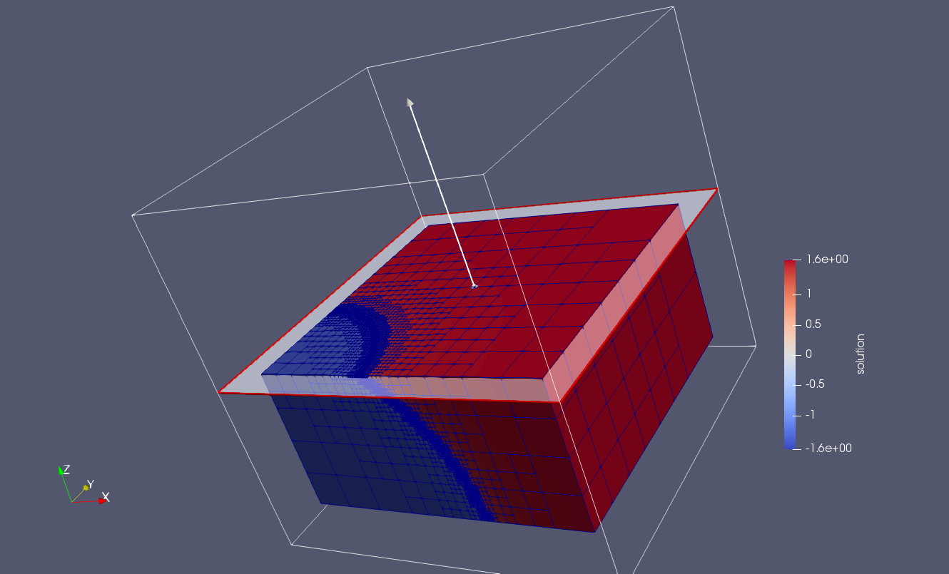
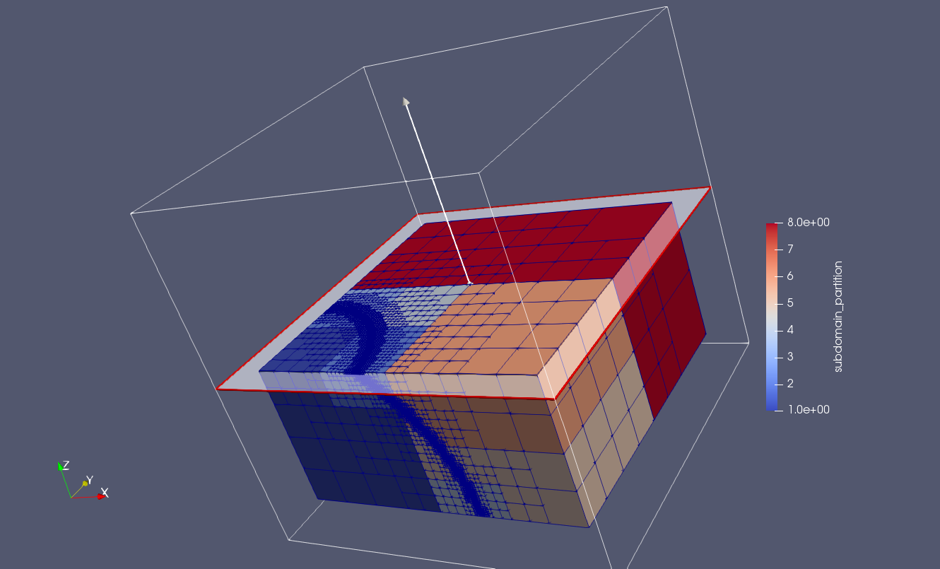
Figure 6. Mesh and FE solution (left) and its partition into 9 subdomains (right). 13 AMR steps; 218,590 cells; 153,760 (true) DOFs.

8. Conclusions

In this article we have provided three tutorials that cover some of the capabilities of the FEMPAR library. The tutorials come with a comprehensive description of all the steps required in the simulation of PDE-based problems. They cover the numerical approximation of a linear PDE, structured and octree meshes with AMR strategies (both in serial and parallel environments), and the usage of parallel iterative solvers with scalable preconditioning techniques. This set of tutorials provides FEMPAR users with a complete introduction to some key FEMPAR tools. In any case, we refer to the tutorials folder in the FEMPAR public repository https://github.com/fempar/fempar for more advanced topics not covered here (e.g., nonlinear solvers, time integration, curl and div conforming FE spaces, multi-field FE spaces, or block preconditioning techniques).

References

- [1] C. Burstedde, L. C. Wilcox, O. Ghattas, SIAM Journal on Scientific Computing 33 (3) (2011) 1103–1133.
- [2] O. Colomés, S. Badia, R. Codina, J. Principe, Computer Methods in Applied Mechanics and Engineering 285 (2015) 32–63.
- [3] O. Colomés, S. Badia, International Journal for Numerical Methods in Engineering 105 (5) (2016) 372–400.
- [4] O. Colomés, S. Badia, J. Principe, Computer Methods in Applied Mechanics and Engineering 304 (2016) 294–318.
- [5] O. Colomés, S. Badia, Computer Methods in Applied Mechanics and Engineering 313 (2017) 189–215.
- [6] S. Badia, R. Codina, R. Planas, Journal of Computational Physics 234 (0) (2013) 399–416.
- [7] S. Badia, R. Planas, J. V. Gutiérrez-Santacreu, International Journal for Numerical Methods in Engineering 93 (3) (2013) 302–328.
- [8] R. Planas, S. Badia, R. Codina, Journal of Computational Physics 230 (8) (2011) 2977–2996.
- [9] S. Smolentsev, S. Badia, R. Bhattacharyay, L. Bühler, L. Chen, Q. Huang, H.-G. Jin, D. Krasnov, D.-W. Lee, E. M. de les Valls, C. Mistrangelo, R. Munipalli, M.-J. Ni, D. Pashkevich, A. Patel, G. Pulugundla, P. Satyamurthy, A. Snegirev, V. Sviridov, P. Swain, T. Zhou, O. Zikanov, Fusion Engineering and Design 100 (2015) 65–72.
- [10] S. Badia, R. Codina, R. Planas, Archives of Computational Methods in Engineering 22 (4) (2015) 621–636.
- [11] S. Badia, A. Hierro, Computer Methods in Applied Mechanics and Engineering 286 (2015) 107–122.
- [12] S. Badia, A. Hierro, SIAM Journal on Scientific Computing 36 (6) (2014) A2673–A2697.
- [13] A. Hierro, S. Badia, P. Kus, Computer Methods in Applied Mechanics and Engineering 309 (2016) 532–553.
- [14] S. Badia, J. Bonilla, Computer Methods in Applied Mechanics and Engineering 313 (2017) 133–158.
- [15] S. Badia, J. Bonilla, A. Hierro, Computer Methods in Applied Mechanics and Engineering 320 (2017) 582–605.
- [16] S. Badia, A. F. Martin, F. Verdugo, SIAM Journal on Scientific Computing 40 (6) (2018) B1541–B1576.
- [17] F. Verdugo, A. F. Martín, S. Badia, arXiv.arXiv:1902.01168.
- [18] M. Chiumenti, E. Neiva, E. Salsi, M. Cervera, S. Badia, J. Moya, Z. Chen, C. Lee, C. Davies, Additive Manufacturing 18 (2017) 171–185.
- [19] E. Neiva, M. Chiumenti, M. Cervera, E. Salsi, G. Piscopo, S. Badia, A. F. Martín, Z. Chen, C. Lee, C. Davies, arXiv.arXiv:1811.12372.
- [20] E. Neiva, S. Badia, A. F. Martín, M. Chiumenti, International Journal for Numerical Methods in Engineering (2019) nme.6085.
- [21] M. Olm, S. Badia, A. F. Martín, Computer Physics Communications 237 (2019) 154–167.
- [22] M. Olm, S. Badia, A. F. Martín, Advances in Engineering Software 132 (2019) 74–91.
- [23] S. Badia, A. F. Martín, J. Principe, Parallel Computing 50 (2015) 1–24.
- [24] S. Badia, A. F. Martín, J. Principe, SIAM Journal on Scientific Computing (2016) C22–C52.
- [25] S. Balay, S. Abhyankar, M. F. Adams, J. Brown, P. Brune, K. Buschelman, L. Dalcin, V. Eijkhout, W. D. Gropp, D. Kaushik, M. G. Knepley, L. C. McInnes, K. Rupp, B. F. Smith, S. Zampini, H. Zhang, H. Zhang, 2016.
- [26] H. C. Elman, D. J. Silvester, A. J. Wathen, Oxford University Press, 2005.
- [27] S. Badia, A. F. Martín, J. Principe, Archives of Computational Methods in Engineering 20 (3) (2013) 239–262.
- [28] S. Badia, A. F. Martín, J. Príncipe, International Journal for Numerical Methods in Engineering 96 (4) (2013) 203–230.
- [29] S. Badia, H. Nguyen, SIAM Journal on Numerical Analysis 54 (6) (2016) 3436–3464.
- [30] S. Badia, A. F. Martín, H. Nguyen, Journal of Scientific Computing 79 (2) (2019) 718–747.
- [31] S. Badia, A. F. Martín, J. Principe, SIAM Journal on Scientific Computing 36 (2) (2014) C190–C218.
- [32] S. Badia, M. Olm, SIAM Journal on Scientific Computing 39 (2) (2017) C194–C213.
- [33] S. Badia, F. Verdugo, Journal of Computational and Applied Mathematics 344 (2018) 740–759.
- [34] S. Badia, A. F. Martín, H. Nguyen, Applied Mathematics Letters 87 (2019) 93–100.
- [35] S. Badia, A. F. Martín, M. Olm, Finite Elements in Analysis and Design 161 (2019) 16–31.
- [36] S. Badia, A. F. Martín, R. Planas, Journal of Computational Physics 274 (2014) 562–591.
- [37] S. Badia, A. F. Martín, J. Principe, Archives of Computational Methods in Engineering 25 (2) (2018) 195–271.
- [38] GiD–the personal pre and post processor, http://www.gidhome.com.
- [39] Gamma, E., Helm, R., Johnson, R., Vlissides, J., Addison-Wesley, 1995.
- [40] E. Freeman, E. Robson, K. Sierra, B. Bates (Eds.), O’Reilly, Sebastopol, CA, 2004.
- [41] FPL -- Fortran parameter list, https://gitlab.com/fempar/FPL.
- [42] W. F. Mitchell, M. A. McClain, A Survey of hp-Adaptive Strategies for Elliptic Partial Differential Equations, in: Recent Advances in Computational and Applied Mathematics, Springer Netherlands, Dordrecht, 2011, pp. 227--258.
- [43] A. Quarteroni, Springer Milan, Milano, 2014.
- [44] Intel MKL PARDISO - Parallel Direct Sparse Solver Interface, https://software.intel.com/en-us/articles/intel-mkl-pardiso.
- [45] T. A. Davis, T. A., ACM Transactions on Mathematical Software 30 (2) (2004) 196--199.
- [46] W. Schroeder, K. M. Martin, W. E. Lorensen, Prentice-Hall, Inc., Upper Saddle River, NJ, USA, 1998.
- [47] XDMF -- eXtensible Data Model and Format, http://www.xdmf.org/index.php/Main_Page.
- [48] S. Badia, A. F. Martín, E. Neiva, F. Verdugo, arXiv.arXiv:1907.03709.
- [49] L.-y. Li, P. Bettess, Applied Mechanics Reviews 50 (10) (1997) 581.
- [50] Y. Saad, 2nd Edition, Society for Industrial and Applied Mathematics, 2003.
- [51] A. Toselli, O. Widlund, Springer-Verlag, 2005.
- [52] S. Badia, A. F. Martín, J. Principe, SIAM Journal on Scientific Computing (2014) C190--C218.
- [53] S. Zampini, SIAM J. Sci. Comput. 38 (2016) S282--S306.
- [54] S. C. Brenner, R. Scott, softcover reprint of hardcover 3rd ed. 2008 Edition, Springer, 2010.
- [55] C. R. Dohrmann, SIAM Journal on Scientific Computing 25 (1) (2003) 246--258.
- [56] J. Mandel, B. Sousedík, C. Dohrmann, Computing 83 (2) (2008) 55--85.
- [57] P. Kus, J. Sistek, Advances in Engineering Software 110 (2017) 34--54. arXiv:1703.06494.