Site-occupation–Green’s function embedding theory: A density-functional approach to dynamical impurity solvers

Abstract

A reformulation of site-occupation embedding theory (SOET) in terms of Green’s functions is presented. Referred to as site-occupation–Green’s function embedding theory (SOGET), this novel extension of density-functional theory for model Hamiltonians shares many features with dynamical mean-field theory (DMFT) but is formally exact (in any dimension). In SOGET, the impurity-interacting correlation potential becomes a density-functional self-energy which is frequency-dependent and in principle non-local. A simple local density-functional approximation (LDA) combining the Bethe Ansatz (BA) LDA with the self-energy of the two-level Anderson model is constructed and successfully applied to the one-dimensional Hubbard model. Unlike in previous implementations of SOET, no many-body wavefunction is needed, thus reducing drastically the computational cost of the method.

I Introduction

The description of strong electron correlation is a long-standing problem in both quantum chemistry and condensed matter physics. In the former case, state-of-the-art ab initio methods are based on the explicit calculation of a many-body wavefunction. Unfortunately, they can only be applied to relatively small systems because of the exponentially increasing size of the many-body Hilbert space. An in-principle-exact alternative is density-functional theory (DFT) Hohenberg and Kohn (1964); Kohn and Sham (1965) which drastically reduces the cost by mapping the fully interacting system onto a non-interacting one. The bottleneck of DFT is, in practice, the lack of accurate density-functional approximations that can properly treat strongly correlated systems Cohen et al. (2012); Swart (2013); Swart and Gruden (2016). In the face of these problems, new methods have been developed. Due to the fact that strong electron correlation is mainly local, only a reduced part of the system has to be treated accurately. Hence, quantum embedding methods Sun and Chan (2016); Mühlbach and Reiher (2018) have been gaining an increasing attention. They deliver a good compromise between the accuracy of wavefunction-based methods and the computational cost of mean-field-like methods like DFT.

Turning to model Hamiltonians like Hubbard, the Green’s function-based dynamical mean-field theory (DMFT) Georges and Kotliar (1992); Georges et al. (1996); Kotliar and Vollhardt (2004); Held (2007); Zgid and Chan (2011) is exact in the infinite dimension limit where the self-energy is momentum-independent and local. When merged with ab initio approaches like DFT Kotliar et al. (2006) or GW Sun and Kotliar (2002); Biermann et al. (2003); Karlsson (2005); Boehnke et al. (2016); Werner and Casula (2016); Nilsson et al. (2017), the method can be applied to realistic systems. DMFT has been succesfull in describing materials with localized $d$ and $f$ bands Haule et al. (2008); Miyake et al. (2008). An appealing extension of Green’s function techniques to quantum chemical problems is self-energy embedding theory (SEET)  Kananenka et al. (2015); Lan et al. (2015); Zgid and Gull (2017); Lan and Zgid (2017) where local and non-local electronic correlations are modelled by the combination of wave function-based methods with many-body perturbation theory. A mixture of configuration interaction with Green’s functions has also been recently proposed by Dvorak and Rinke Dvorak and Rinke (2019).

For the calculation of non-dynamical properties, density matrix embedding theory (DMET)  Knizia and Chan (2012, 2013); Bulik et al. (2014); Zheng and Chan (2016); Wouters et al. (2016); Rubin (2016); Welborn et al. (2016); Wouters et al. (2017); Ye et al. (2018); Fertitta and Booth (2018), or the related rotationally invariant slave bosons technique Ayral et al. (2017); Lee et al. (2019), has become a viable alternative to DMFT. In standard DMET, the embedding procedure relies on the Schmidt decomposition of a mean-field many-body wavefunction. The one-electron reduced density matrix is then introduced in order to define a convergence criterion for the method. Note that DMET has also been extended to the calculation of spectral properties Booth and Chan (2015).

Turning now to DFT for model Hamiltonians, also referred to as site-occupation functional theory (SOFT) Capelle and Campo (2013), a local density approximation (LDA) based on the Bethe ansatz (BA) has been developed for the one-dimensional (1D) Hubbard model Lima et al. (2002, 2003); Capelle et al. (2003). It contains the effect of strong correlation and can describe Mott physics Silva et al. (2005); Akande and Sanvito (2010). An extension of BALDA to higher dimensions has been recently proposed Vilela et al. (2019). Note also that the use of other (frequency-independent) reduced quantities, such as the one-body density matrix, has been considered in the so-called lattice DFT López-Sandoval and Pastor (2002, 2004); Saubanère and Pastor (2009); Töws and Pastor (2011); Saubanère and Pastor (2011); Töws et al. (2013); Saubanère et al. (2016). In recent years, an in-principle-exact alternative formulation of SOFT, referred to as site-occupation embedding theory (SOET) Fromager (2015); Senjean et al. (2017, 2018a, 2018b), has been explored. In contrast to standard Kohn–Sham (KS) DFT, SOET maps the whole physical system onto an impurity-interacting one. Note that both systems have the same size. So far, the impurity-interacting system has been treated by exact diagonalization for small rings Senjean et al. (2017) or on the level of density matrix renormalization group (DMRG) Nakatani ; Senjean et al. (2018a) for (slightly) larger systems. More recently, Senjean has formulated a projected version of SOET, where the Schmidt decomposition is applied to the KS determinant, thus reducing drastically the computational cost of the method Senjean (2019). In order to access physical properties such as double occupations and per-site energies, a density-functional correction is applied to the “bare” properties of the auxiliary impurity-interacting system Senjean et al. (2018a). The formal advantages of SOET over other hybrid methods is the absence of double counting, the existence of a variational principle, as well as in-principle-exact expressions for the physical properties of interest. From a practical point of view, the major drawback of SOET is the size of the impurity-interacting system which is not effectively reduced as in DMET and makes calculations prohibitively expensive.

As mentioned previously, a reduction in system size can be obtained by projection Senjean (2019), in the spirit of DMET. In this work, we explore an alternative approach based on the reformulation of SOET in terms of Green’s functions. The approach will be referred to as site-occupation–Green’s function embedding theory (SOGET) in the following. Instead of combining static density-functional approximations with a many-body wavefunction treatment, we introduce in SOGET a density-functional self-energy which is both frequency- and site-occupation-dependent. The role of this self-energy is to generate an impurity Green’s function that reproduces, in principle exactly, the site occupations of the physical system. It also describes electron correlation in the auxiliary impurity-interacting system. In this work, we develop a simple LDA based on the combination of BALDA with the Anderson dimer model. As our self-energy depends explicitly on the impurity site occupation, there is no need for an impurity solver, thus reducing drastically the computational cost of the method.

The paper is organized as follows. After a brief review on SOET (Sec. II.1), a formally exact derivation of SOGET is presented in Sec. II.2. The importance of derivative discontinuities in the bath, when it comes to model gap openings, is then highlighted in Sec. II.3. In order to turn SOGET into a practical computational method, density-functional approximations to both correlation energies and the impurity-interacting self-energy must be developed, as discussed in detail in Sec. III. A summary of the various approximations as well as computational details are given in Sec. IV. Results obtained with SOGET for the 1D Hubbard model are presented and discussed in Sec. V. Conclusions and perspectives are finally given in Sec. VI.

II Theory

II.1 Site-occupation embedding theory

The single-impurity version of SOET, which is considered in the rest of this work, is briefly reviewed in the following. More details can be found in Refs. Senjean et al. (2018a, b). We start from the (grand canonical) 1D Hubbard Hamiltonian,

$$\hat{H}=\hat{T}+\hat{U}+\hat{V}-\mu\hat{N},$$ (1)

where

$$\hat{T}=-t\displaystyle{\sum_{<i,j>,\sigma}}(\hat{a}_{i\sigma}^{\dagger}\hat{a}_{j\sigma}+\mathrm{h.c.})$$ (2)

describes the nearest-neighbor hopping of the electrons. It is analogous to the kinetic energy operator in DFT. The parameter $t$ is the hopping integral. The summation over site indices goes from $i=0$ to $L-1$. In order to uniquely define the ground state, we impose anti-periodic boundary conditions ($\hat{a}_{L\sigma}=-\hat{a}_{0\sigma}$) when the number of electrons is a multiple of four and periodic boundary conditions ($\hat{a}_{L\sigma}=\hat{a}_{0\sigma}$) otherwise. The Coulomb operator

$$\hat{U}=U\displaystyle{\sum_{i}}\hat{n}_{i\uparrow}\hat{n}_{i\downarrow}$$ (3)

describes the on-site repulsion of electrons with interaction strength $U$. In addition to the kinetic and Coulomb term, we add a local potential operator

$$\hat{V}=\sum_{i}v_{i}\hat{n}_{i}$$ (4)

which plays the role of the external potential in DFT and therefore modulates the electronic density (the occupation of the sites in this context). The density operator on site $i$,

$$\hat{n}_{i}=\sum_{\sigma}\hat{a}_{i\sigma}^{\dagger}\hat{a}_{i\sigma},$$ (5)

yields the individual site occupations which can be viewed as a proxy of the electronic density in atomic systems. The chemical potential $\mu$ fixes the total number of electrons in the system via the particle number operator

$$\hat{N}=\sum_{i}\hat{n}_{i}\,.$$ (6)

In the language of DFT Hohenberg and Kohn (1964), the exact ground-state energy is obtained variationally, and for a given number of electrons, as follows:

$$E(\mathbf{v})=\min_{\mathbf{n}}\{F(\mathbf{n})+(\mathbf{v}|\mathbf{n})\},$$ (7)

where $\mathbf{n}\equiv(n_{0},n_{1},\ldots,n_{L-1})$ is the density profile,

$$F(\mathbf{n})=\min_{\Psi\rightarrow\mathbf{n}}\langle\Psi|\big{(}\hat{T}+\hat{U}\big{)}|\Psi\rangle$$ (8)

is the Levy-Lieb (LL) functional, and

$$(\mathbf{v}|\mathbf{n})=\sum_{i}v_{i}n_{i}\,.$$ (9)

Within the conventional KS formalism, the expression in Eq. (8) is split as follows:

$$F(\mathbf{n})=T_{\rm s}(\mathbf{n})+E_{\rm Hxc}(\mathbf{n}),$$ (10)

where

$$T_{\rm s}(\mathbf{n})=\min_{\Psi\rightarrow\mathbf{n}}\langle\Psi|\hat{T}|\Psi\rangle$$ (11)

is the kinetic energy functional of the fictitious non-interacting KS system with density $\mathbf{n}$ and

$$E_{\rm Hxc}(\mathbf{n})=\dfrac{U}{4}\sum_{i}n_{i}^{2}+E_{\rm c}(\mathbf{n})$$ (12)

is the Hartree-exchange-correlation (Hxc) functional. In the particular case of a uniform system, which is considered in the rest of this work, the following local density approximation to the correlation energy becomes exact:

$$E_{\rm c}(\mathbf{n})=\sum_{i}e_{\rm c}(n_{i}),$$ (13)

where $e_{\rm c}(n)$ is the per-site density-functional correlation energy.

In SOET, a different partitioning of the LL functional is used,

$$F(\mathbf{n})=F^{\rm imp}(\mathbf{n})+\overline{E}_{\rm Hxc}^{\rm bath}(\mathbf{n}),$$ (14)

where

$$F^{\rm imp}(\mathbf{n}) = \min_{\Psi\rightarrow\mathbf{n}}\langle\Psi|\big{(}\hat{T}+\hat{U}_{0})|\Psi\rangle,$$ (15)

$$= \left\langle\Psi^{\rm imp}(\mathbf{n})\middle|\hat{T}+\hat{U}_{0}\middle|\Psi^{\rm imp}(\mathbf{n})\right\rangle,$$

and $\hat{U}_{0}=U\hat{n}_{0\uparrow}\hat{n}_{0\downarrow}$. The latter functional is the analog of the LL functional for a partially-interacting system where the on-site Coulomb interaction $U$ is switched off on the whole lattice except on one site labelled as $i=0$. The latter is referred to as the “impurity” whereas the region of all the remaining (non-interacting) sites is called “bath” in SOET. Note that, if $\mathbf{n}$ is pure-state impurity-interacting $v$-representable, the minimizing wavefunction $\Psi^{\rm imp}(\mathbf{n})$ in Eq. (15) is well-defined and it fulfills the following ground-state Schrödinger-like equation:

$$\hat{H}^{\rm imp}(\mathbf{n})\left|\Psi^{\rm imp}(\mathbf{n})\right\rangle=\mathcal{E}^{\rm imp}(\mathbf{n})\left|\Psi^{\rm imp}(\mathbf{n})\right\rangle,$$ (16)

where the impurity-interacting density-functional Hamiltonian reads

$$\hat{H}^{\rm imp}(\mathbf{n})=\hat{T}+\hat{U}_{0}+\sum_{i}v_{i}^{\rm emb}(\mathbf{n})\,\hat{n}_{i}.$$ (17)

The unicity (up to a constant) of the potential $\left\{v_{i}^{\rm emb}(\mathbf{n})\right\}_{0\leq i\leq L-1}$ is guaranteed by the Hohenberg–Kohn theorem Hohenberg and Kohn (1964) that we simply apply in this context to impurity-interacting Hamiltonians.

The second term on the right-hand side of Eq. (14) is the Hxc functional of the bath. It can be decomposed into Hx and correlation terms as follows,

$$\overline{E}_{\rm Hxc}^{\rm bath}(\mathbf{n})=\dfrac{U}{4}\sum_{i\neq 0}n_{i}^{2}+\overline{E}_{\rm c}^{\rm bath}(\mathbf{n}).$$ (18)

If we consider the KS decomposition of the impurity-interacting LL functional $F^{\rm imp}(\mathbf{n})=T_{\rm s}(\mathbf{n})+E_{\rm Hxc}^{\rm imp}(\mathbf{n})$, where $E_{\rm Hxc}^{\rm imp}(\mathbf{n})=({U}n^{2}_{0}/4)+E_{\rm c}^{\rm imp}(\mathbf{n})$, it comes

$$\overline{E}^{\rm bath}_{\rm c}(\mathbf{n})=E_{\rm c}(\mathbf{n})-E_{\rm c}^{\rm imp}(\mathbf{n}),$$ (19)

where we readily see that the complementary bath correlation functional describes not only the correlation in the bath but also its coupling with the correlation effects on the impurity.

By inserting Eqs. (14) and (15) into Eq. (7), it can be shown Senjean et al. (2018a) that, in SOET, the KS equations are replaced by the following self-consistent ground-state many-body wavefunction equation,

$$\left(\hat{T}+\hat{U}_{0}+\sum_{i}v_{i}^{\rm emb}\hat{n}_{i}\right)|\Psi^{\rm imp}\rangle=\mathcal{E}^{\rm imp}|\Psi^{\rm imp}\rangle,$$ (20)

where

$$v_{i}^{\rm emb}=v_{i}+\left.\frac{\partial\overline{E}^{\rm bath}_{\rm Hxc}(\mathbf{n})}{\partial n_{i}}\right|_{\mathbf{n}=\mathbf{n}^{\Psi^{\rm imp}}}-\mu$$ (21)

plays the role of a density-functional embedding potential for the impurity. It ensures that the impurity-interacting wavefunction yields the site-occupation of the physical Hubbard model. Note that, like in DFT, the latter (auxiliary) wavefunction is not expected to reproduce other observables such as the double occupation. One needs to add the density-functional contributions from the bath [see Eq. (19)] to the bare impurity-interacting double occupation $d^{\rm imp}$ in order to calculate in-principle-exact and physically meaningful properties. In the particular case of the uniform Hubbard model, i.e. when $\mathbf{n}^{\Psi^{\rm imp}}\equiv(n,n,\ldots,n)$, the exact double occupation reads as follows in SOET: Senjean et al. (2018a)

$$d=d^{\rm imp}+\dfrac{\partial\overline{e}_{\rm c}^{\rm bath}(\mathbf{n}^{\Psi^{\rm imp}})}{\partial U},$$ (22)

where

$$d^{\rm imp}=\langle\Psi^{\rm imp}|\hat{n}_{0\uparrow}\hat{n}_{0\downarrow}|\Psi^{\rm imp}\rangle,$$ (23)

and

$$\overline{e}_{\rm c}^{\rm bath}(\mathbf{n}) = e_{\rm c}({n}_{0})-E^{\rm imp}_{\rm c}(\mathbf{n})$$ (24)

$$= \overline{E}^{\rm bath}_{\rm c}(\mathbf{n})-\sum_{i\neq 0}e_{\rm c}({n}_{i}).$$

The latter functional can be seen as a per-site correlation functional for the bath. The exact physical per-site energy can be expressed as follows Senjean et al. (2018a, b):

$$e = t_{\rm s}({n})+t\frac{\partial e_{\rm c}(n)}{\partial t}+Ud^{\rm imp}+U\frac{\partial\overline{e}_{\rm c}^{\rm bath}(\mathbf{n}^{\Psi^{\rm imp}})}{\partial U}\,,$$ (25)

where $t_{\rm s}(n)$ is the non-interacting per-site kinetic energy functional [$t_{\rm s}(n)=-4t\sin(\pi n/2)/\pi$ in the 1D case].

II.2 Site-occupation–Green’s function embedding theory

II.2.1 Density-functional self-energy

In the following, we propose a complete reformulation and simplication of SOET based on the Green’s function formalism. We would like the embedding procedure to remain a functional of the density, unlike in conventional approaches like DMFT or SEET where the Green’s function is the basic variable. For that purpose, we start from the impurity-interacting many-body wavefunction in Eq. (16) and consider the corresponding (retarded) equilibrium zero-temperature frequency-dependent one-particle Green’s function ${\bf G}^{\rm imp}\left(\mathbf{n},\omega\right)\equiv\left\{G^{\rm imp}_{i\sigma,j\sigma^{\prime}}\left(\mathbf{n},\omega\right)\right\}_{i,j,\sigma,\sigma^{\prime}}$ with $0\leq i,j\leq L-1$, which we simply refer to as the impurity Green’s function in the following. Its elements in the Lehmann representation are defined as follows:

$$G^{\rm imp}_{i\sigma,j\sigma^{\prime}}\left(\mathbf{n},\omega\right) = \left\langle\hat{a}_{i\sigma}\frac{1}{\omega+\mathcal{E}^{\rm imp}(\mathbf{n})-\hat{H}^{\rm imp}(\mathbf{n})+{\rm i}\eta}\hat{a}_{j\sigma^{\prime}}^{\dagger}\right\rangle_{\Psi^{\rm imp}(\mathbf{n})}+\left\langle\hat{a}_{j\sigma^{\prime}}^{\dagger}\frac{1}{\omega-\mathcal{E}^{\rm imp}(\mathbf{n})+\hat{H}^{\rm imp}(\mathbf{n})+{\rm i}\eta}\hat{a}_{i\sigma}\right\rangle_{\Psi^{\rm imp}(\mathbf{n})},$$

where $\eta\rightarrow 0^{+}$. Note that, by construction, the impurity Green’s function reproduces the density profile ${\bf n}$:

$$-\frac{1}{\pi}\sum_{\sigma}\int_{-\infty}^{0}{d}\omega\,\mathrm{Im}\,\left[G_{i\sigma,i\sigma}^{\rm imp}\left(\mathbf{n},\omega\right)\right]=n_{i},$$ (27)

where we integrate up to zero since the chemical potential is included into $\hat{H}^{\rm imp}(\mathbf{n})$. Note also that, by analogy with the fully-interacting case [see Eq. (A.1) in Ref. Potthoff, M. (2003)], one could make the one-to-one correspondence between the impurity-interacting Green’s function and the embedding potential (which is itself an implicit functional of the ground-state density) more explicit by expanding the Green’s function through second order in $1/\omega$.

Let us now introduce an auxiliary interaction-free Green’s function $\mathbfcal{G}^{\rm imp}\left(\mathbf{n},\omega\right)$ which is obtained by removing from $\hat{H}^{\rm imp}(\mathbf{n})$ the interaction on the impurity site. From the point of view of DMFT, $\mathbfcal{G}^{\rm imp}\left(\mathbf{n},\omega\right)$ might be seen as a density-functional Weiss field, whose explicit expression reads

$$\mathbfcal{G}^{\rm imp}\left(\mathbf{n},\omega\right)=\left[\left(\omega+{\rm i}\eta\right)\mathbf{I}-\mathbf{t}-\mathbf{v}^{\rm emb}(\mathbf{n})\right]^{-1},$$

where $\mathbf{I}$ is the identity matrix, $\mathbf{t}$ is the matrix representation of the (one-electron) hopping operator, and $\mathbf{v}^{\rm emb}(\mathbf{n})\equiv\left\{\delta_{\sigma\sigma^{\prime}}\delta_{ij}v_{i}^{\rm emb}(\mathbf{n})\right\}_{0\leq i,j\leq L-1,\sigma,\sigma^{\prime}}$ is the matrix representation of the local and frequency-independent embedding potential. Note that $\mathbfcal{G}^{\rm imp}\left(\mathbf{n},\omega\right)$ is a functional of the density $\mathbf{n}$ but it does not reproduce that density.

We can now define a density-functional impurity self-energy,

$$\mathbf{\Sigma}_{\rm Hxc}^{\rm imp}(\mathbf{n},\omega)=\left[\mathbfcal{G}^{\rm imp}\left(\mathbf{n},\omega\right)\right]^{-1}-\left[\mathbf{G}^{\rm imp}\left(\mathbf{n},\omega\right)\right]^{-1},$$

(29)

which is (one of) the central quantity in SOGET. It is in principle non-local and, when combined with the impurity Green’s function, it gives access to the impurity LL density-functional energy defined in Eq. (15). Indeed, since real algebra can be used to describe the impurity-interacting density-functional many-body wavefunction $\Psi^{\rm imp}(\mathbf{n})$, its kinetic energy can be written as

$$\langle\Psi^{\rm imp}(\mathbf{n})|\hat{T}|\Psi^{\rm imp}(\mathbf{n})\rangle = -t\displaystyle{\sum_{<i,j>,\sigma}}\left\langle\hat{a}_{i\sigma}^{\dagger}\hat{a}_{j\sigma}+\mathrm{h.c.}\right\rangle_{\Psi^{\rm imp}(\mathbf{n})}$$ (30)

$$= -2t\displaystyle{\sum_{<i,j>,\sigma}}\left\langle\hat{a}_{j\sigma}^{\dagger}\hat{a}_{i\sigma}\right\rangle_{\Psi^{\rm imp}(\mathbf{n})},$$

where, according to Eq. (LABEL:eq:impurity_green_function_lehmann),

$$\left\langle\hat{a}_{j\sigma}^{\dagger}\hat{a}_{i\sigma}\right\rangle_{\Psi^{\rm imp}(\mathbf{n})} = -\dfrac{1}{\pi}\int_{-\infty}^{0}{d}\omega\,\mathrm{Im}\,\left[G_{i\sigma,j\sigma}^{\rm imp}\left(\mathbf{n},\omega\right)\right].$$

We stress again that the chemical potential is included into $\hat{H}^{\rm imp}(\mathbf{n})$, hence the integration up to zero in Eq. (II.2.1). In addition, by deriving the equation of motion for the impurity-interacting Green’s function, it can be shown, in complete analogy with conventional Green’s function theory, that the density-functional impurity interaction energy reads

$$\langle\Psi^{\rm imp}(\mathbf{n})|\hat{U}_{0}|\Psi^{\rm imp}(\mathbf{n})\rangle=U\left\langle\hat{n}_{0\uparrow}\hat{n}_{0\downarrow}\right\rangle_{\Psi^{\rm imp}(\mathbf{n})}$$

$$=-\dfrac{1}{\pi}\int_{-\infty}^{0}{d}\omega\,\mathrm{Im}\,\left[\mathbf{\Sigma}_{\rm Hxc}^{\rm imp}(\mathbf{n},\omega)\mathbf{G}^{\rm imp}\left(\mathbf{n},\omega\right)\right]_{0\sigma^{\prime},0\sigma^{\prime}},$$ (32)

where $\sigma^{\prime}$ refers to a spin up or spin down state [for simplicity, we restrict the discussion to cases where the Green’s function is the same for up and down spins]. From Eqs. (15), (30), (II.2.1) and (II.2.1), we obtain the following expression:

$$F^{\rm imp}(\mathbf{n})=\frac{2t}{\pi}\sum_{<i,j>,\sigma}\int_{-\infty}^{0}{d}\omega\,\mathrm{Im}\,\left[G_{i\sigma,j\sigma}^{\rm imp}\left(\mathbf{n},\omega\right)\right]$$

$$-\dfrac{1}{\pi}\int_{-\infty}^{0}{d}\omega\,\mathrm{Im}\,\left[\mathbf{\Sigma}_{\rm Hxc}^{\rm imp}(\mathbf{n},\omega)\mathbf{G}^{\rm imp}\left(\mathbf{n},\omega\right)\right]_{0\sigma^{\prime},0\sigma^{\prime}}.$$ (33)

Combining Eq. (II.2.1) with Eq. (14) leads to a formally exact SOGET where, like in SOET, the bath is described with a density functional and, unlike in SOET, a Green’s function is used to describe the impurity-interacting system (instead of a many-body wavefunction).

Interestingly, if we introduce the KS potential into the density-functional embedding one [see Eqs. (19) and (21)],

$$v_{i}^{\rm emb}(\mathbf{n}) = v_{i}^{\rm KS}(\mathbf{n})-\frac{\partial{E}_{\rm Hxc}(\mathbf{n})}{\partial n_{i}}+\frac{\partial\overline{E}^{\rm bath}_{\rm Hxc}(\mathbf{n})}{\partial n_{i}}$$ (34)

$$= v_{i}^{\rm KS}(\mathbf{n})-\frac{\partial{E}^{\rm imp}_{\rm Hxc}(\mathbf{n})}{\partial n_{i}}$$

$$= v_{i}^{\rm KS}(\mathbf{n})-v^{\rm imp}_{{\rm Hxc},i}(\mathbf{n}),$$

we deduce from Eqs. (II.2.1) and (29) the following Dyson equation,

$$\mathbf{\Sigma}_{\rm Hxc}^{\rm imp}(\mathbf{n},\omega) = \left[\mathbf{G}^{\rm KS}\left(\mathbf{n},\omega\right)\right]^{-1}-\left[\mathbf{G}^{\rm imp}\left(\mathbf{n},\omega\right)\right]^{-1}$$ (35)

$$+{\mathbf{v}}_{\rm Hxc}^{\rm imp}(\mathbf{n}),$$

or, equivalently,

$$\mathbf{G}^{\rm imp}\left(\mathbf{n},\omega\right)=\mathbf{G}^{\rm KS}\left(\mathbf{n},\omega\right)$$

$$+\mathbf{G}^{\rm KS}\left(\mathbf{n},\omega\right)\left(\mathbf{\Sigma}_{\rm Hxc}^{\rm imp}(\mathbf{n},\omega)-{\mathbf{v}}_{\rm Hxc}^{\rm imp}(\mathbf{n})\right)\mathbf{G}^{\rm imp}\left(\mathbf{n},\omega\right),$$

where $\mathbf{G}^{\rm KS}\left(\mathbf{n},\omega\right)=\left[\left(\omega+{\rm i}\eta\right)\mathbf{I}-\mathbf{t}-\mathbf{v}^{\rm KS}(\mathbf{n})\right]^{-1}$ is the non-interacting KS Green’s function. Comparing Eq. (35) with Eqs. (16), (17), and (34) reveals a key difference between SOET and SOGET. While the former generates the impurity-interacting many-body wavefunction with density $\mathbf{n}$ from the local and frequency-independent potential ${\mathbf{v}}_{\rm Hxc}^{\rm imp}(\mathbf{n})$, SOGET is expected to generate the corresponding Green’s function from the KS one. For that purpose, non-local and frequency-dependent corrections to ${\mathbf{v}}_{\rm Hxc}^{\rm imp}(\mathbf{n})$ are in principle needed. These corrections will be contained in the correlation part of the impurity-interacting self-energy that needs to be modelled.

Finally, since the KS and impurity-interacting Green’s functions reproduce the same density profile ${\bf n}$, i.e.

$$\sum_{\sigma}\int_{-\infty}^{0}{d}\omega\,\mathrm{Im}\,\left[G_{i\sigma,i\sigma}^{\rm imp}\left(\mathbf{n},\omega\right)\right]$$

$$= \sum_{\sigma}\int_{-\infty}^{0}{d}\omega\,\mathrm{Im}\,\left[G_{i\sigma,i\sigma}^{\rm KS}\left(\mathbf{n},\omega\right)\right],$$ (37)

we obtain, by inserting Eq. (II.2.1) into Eq. (II.2.1), a Sham–Schlüter-like equation for the impurity-interacting system:

$$\sum_{\sigma}\int_{-\infty}^{0}{d}\omega\,\mathrm{Im}\,\left[\mathbf{G}^{\rm KS}\left(\mathbf{n},\omega\right)\mathbf{\Sigma}_{\rm Hxc}^{\rm imp}(\mathbf{n},\omega)\mathbf{G}^{\rm imp}\left(\mathbf{n},\omega\right)\right]_{i\sigma,i\sigma}=\sum_{\sigma,j}{v}_{{\rm Hxc},j}^{\rm imp}(\mathbf{n})\int_{-\infty}^{0}{d}\omega\,\mathrm{Im}\,\left[{G}_{i\sigma,j\sigma}^{\rm KS}\left(\mathbf{n},\omega\right){G}_{j\sigma,i\sigma}^{\rm imp}\left(\mathbf{n},\omega\right)\right].$$

This relation, which explicitly connects the local and frequency-independent potential ${\mathbf{v}}_{\rm Hxc}^{\rm imp}(\mathbf{n})$ to the non-local and frequency-dependent self-energy $\mathbf{\Sigma}_{\rm Hxc}^{\rm imp}(\mathbf{n},\omega)$, is a stringent condition that could be used, for example, in the development of approximate embedding potentials. This is left for future work.

II.2.2 Self-consistency loop in SOGET

We explain in this section how the impurity-interacting Green’s function can be determined self-consistently from the density-functional impurity self-energy. Our starting point will be the SOET Eq. (20) where the quantity to be determined self-consistently is the impurity-interacting many-body wavefunction. We want to bypass this step, which is computationally demanding, and propose an alternative equation where the unknown quantity is the corresponding Green’s function.

Let us assume that we have at hand both the correlation functional for the bath and the impurity density-functional self-energy (these two quantities will of course be approximated later on). We denote $\mathbf{G}^{\rm imp}\left(\omega\right)$ the Green’s function constructed from the solution $\Psi^{\rm imp}$ to the self-consistent SOET Eq. (20),

$$G^{\rm imp}_{i\sigma,j\sigma^{\prime}}\left(\omega\right)=\left\langle\hat{a}_{i\sigma}\frac{1}{\omega+\mathcal{E}^{\rm imp}-\hat{H}^{\rm imp}+{\rm i}\eta}\hat{a}_{j\sigma^{\prime}}^{\dagger}\right\rangle_{\Psi^{\rm imp}}$$

$$+\left\langle\hat{a}_{j\sigma^{\prime}}^{\dagger}\frac{1}{\omega-\mathcal{E}^{\rm imp}+\hat{H}^{\rm imp}+{\rm i}\eta}\hat{a}_{i\sigma}\right\rangle_{\Psi^{\rm imp}},$$ (39)

where

$$\hat{H}^{\rm imp}=\hat{T}+\hat{U}_{0}$$

$$+\sum_{i}\left[v_{i}-\mu+\left.\frac{\partial\overline{E}^{\rm bath}_{\rm Hxc}(\mathbf{n})}{\partial n_{i}}\right|_{\mathbf{n}=\mathbf{n}^{\Psi^{\rm imp}}}\right]\hat{n}_{i}.$$ (40)

By construction, the density profile ${\mathbf{n}}^{\mathbf{G}^{\rm imp}}\equiv\left\{n_{i}^{\mathbf{G}^{\rm imp}}\right\}_{0\leq i\leq L-1}$ generated from $\mathbf{G}^{\rm imp}\left(\omega\right)$ equals the density profile of $\Psi^{\rm imp}$:

$$n_{i}^{\mathbf{G}^{\rm imp}} = -\dfrac{1}{\pi}\sum_{\sigma}\int_{-\infty}^{0}{d}\omega\,\mathrm{Im}\,\left[G_{i\sigma,i\sigma}^{\rm imp}\left(\omega\right)\right]$$ (41)

$$= \sum_{\sigma}\bra{\Psi^{\rm imp}}\hat{a}_{i\sigma}^{\dagger}\hat{a}_{i\sigma}\ket{\Psi^{\rm imp}}$$

$$= n_{i}^{\Psi^{\rm imp}},$$

which is itself equal to the density of the physical (Hubbard) system if no approximation is made.

Since, as readily seen from the SOET Eq. (20), $\Psi^{\rm imp}$ is the ground state of an impurity-interacting system with density $\mathbf{n}^{\Psi^{\rm imp}}={\mathbf{n}}^{\mathbf{G}^{\rm imp}}$ and embedding potential

$$\mathbf{v}^{\rm emb}(\mathbf{n}^{\mathbf{G}^{\rm imp}})=\mathbf{v}-\mu+\left.\frac{\partial\overline{E}^{\rm bath}_{\rm Hxc}(\mathbf{n})}{\partial\mathbf{n}}\right|_{\mathbf{n}=\mathbf{n}^{\mathbf{G}^{\rm imp}}},$$ (42)

we conclude [see Eq. (17)] that

$$\hat{H}^{\rm imp}\left(\mathbf{n}^{\mathbf{G}^{\rm imp}}\right)=\hat{H}^{\rm imp},$$ (43)

thus leading to

$$\Psi^{\rm imp}\left(\mathbf{n}^{\mathbf{G}^{\rm imp}}\right) = \Psi^{\rm imp},$$

$$\mathcal{E}^{\rm imp}\left(\mathbf{n}^{\mathbf{G}^{\rm imp}}\right) = \mathcal{E}^{\rm imp},$$ (44)

so that [see Eqs. (LABEL:eq:impurity_green_function_lehmann) and (39)],

$$\mathbf{G}^{\rm imp}\left({\mathbf{n}}^{\mathbf{G}^{\rm imp}},\omega\right)=\mathbf{G}^{\rm imp}\left(\omega\right).$$ (45)

Finally, the latter equation can be rewritten as [see Eq. (29)]

$$\left[\mathbf{G}^{\rm imp}\left(\omega\right)\right]^{-1} = \left[\mathbf{G}^{\rm imp}\left({\mathbf{n}}^{\mathbf{G}^{\rm imp}},\omega\right)\right]^{-1}$$

$$= \left[\mathbfcal{G}^{\rm imp}\left(\mathbf{n}^{\mathbf{G}^{\rm imp}},\omega\right)\right]^{-1}-\mathbf{\Sigma}_{\rm Hxc}^{\rm imp}\left(\mathbf{n}^{\mathbf{G}^{\rm imp}},\omega\right),$$

or, equivalently [see Eqs. (II.2.1) and (42)],

$$\left[\mathbf{G}^{\rm imp}\left(\omega\right)\right]^{-1} = \left[\mathbfcal{G}_{\mathbf{v}}^{\rm imp}\left(\mathbf{n}^{\mathbf{G}^{\rm imp}},\omega\right)\right]^{-1}-\mathbf{\Sigma}_{\rm Hxc}^{\rm imp}\left(\mathbf{n}^{\mathbf{G}^{\rm imp}},\omega\right),$$

where the density-functional interaction-free Green’s function $\mathbfcal{G}_{\mathbf{v}}^{\rm imp}\left(\mathbf{n},\omega\right)$ is determined from the physical external potential $\mathbf{v}$ as follows,

$$\mathbfcal{G}_{\mathbf{v}}^{\rm imp}\left(\mathbf{n},\omega\right)=\left[\left(\omega+\mu+{\rm i}\eta\right)\mathbf{I}-\mathbf{t}-\mathbf{v}-\frac{\partial\overline{E}^{\rm bath}_{\rm Hxc}(\mathbf{n})}{\partial\mathbf{n}}\right]^{-1}.$$

(48)

Thus we conclude that the impurity-interacting Green’s function $\mathbf{G}^{\rm imp}\left(\omega\right)$ fulfills the following self-consistent SOGET equation,

$$\mathbf{\Sigma}_{\rm Hxc}^{\rm imp}\left(\mathbf{n}^{\mathbf{G}},\omega\right)=\left[\mathbfcal{G}_{\mathbf{v}}^{\rm imp}\left(\mathbf{n}^{\mathbf{G}},\omega\right)\right]^{-1}-\left[\mathbf{G}\left(\omega\right)\right]^{-1},$$ (49)

or, equivalently,

$$\mathbf{G}\left(\omega\right)=\left[\left[\mathbfcal{G}_{\mathbf{v}}^{\rm imp}\left(\mathbf{n}^{\mathbf{G}},\omega\right)\right]^{-1}-\mathbf{\Sigma}_{\rm Hxc}^{\rm imp}\left(\mathbf{n}^{\mathbf{G}},\omega\right)\right]^{-1},$$ (50)

which can be seen as an in-principle-exact density-functional version of the self-consistency loop in DMFT. The lighter notation $\mathbf{G}$ (without the superscript “imp”) is used to make the self-consistent character of Eq. (50) more visible.

Turning to uniform systems ($\mathbf{v}\equiv 0$), the self-consistently converged solution to the SOGET Eq. (50) can be combined with the SOET expressions for the double occupation and per-site energy [see Eqs. (22), (25), and (II.2.1)], thus leading to the final SOGET expressions,

$$d = -\dfrac{1}{\pi U}\int_{-\infty}^{0}{d}\omega\,\mathrm{Im}\,\left[\mathbf{\Sigma}_{\rm Hxc}^{\rm imp}\left(\mathbf{n}^{\mathbf{G}^{\rm imp}},\omega\right)\mathbf{G}^{\rm imp}\left(\omega\right)\right]_{0\sigma^{\prime},0\sigma^{\prime}}$$

$$+\dfrac{\partial\overline{e}_{\rm c}^{\rm bath}\left(\mathbf{n}^{\mathbf{G}^{\rm imp}}\right)}{\partial U},$$

(51)

and

$$e = \left[t_{\rm s}({n})+t\frac{\partial e_{\rm c}(n)}{\partial t}\right]_{n={n}_{0}^{\mathbf{G}^{\rm imp}}}+Ud,$$ (52)

where ${n}_{0}^{\mathbf{G}^{\rm imp}}$ is the impurity site occupation.

In addition to the non-locality of the impurity-interacting self-energy (that will be neglected in the rest of this work), the use of a correlation density functional for describing the bath, which is inherited from SOET, plays a crucial role in making SOGET in principle exact, whatever the dimension of the system is. This is an important difference with DMFT, which is only exact in the infinite dimension limit Metzner and Vollhardt (1989). As illustrated in Sec. V, SOGET can actually describe one-dimensional systems accurately.

II.3 Opening of the gap and derivative discontinuities

We discuss in this section the calculation of the chemical potential $\mu\equiv\mu(n)$ as a function of the filling [from now on SOGET is applied to the 1D uniform Hubbard model, i.e. $\mathbf{v}\equiv 0$]. Like in KS-DFT, the impurity-interacting Green’s function of SOGET is expected to reproduce the physical density [the correct filling in this case], not the physical spectral function. Nevertheless, as the former is determined from the latter, we need to explain how the opening of gaps can effectively occur in SOGET. This is a crucial point when it comes to model density-driven Mott–Hubbard transitions (see Sec. V.3). For clarity, we first address this problem in both physical and KS systems, thus highlighting the importance of derivative discontinuities in DFT-based methods.

II.3.1 Physical system

In conventional Green’s function theory, the Green’s function of the physical fully-interacting system fulfills the following self-consistent Dyson equation,

$$\left[\mathbf{G}\left(\omega\right)\right]^{-1} = \left(\omega+\mu+{\rm i}\eta\right)\mathbf{I}-\mathbf{t}-\mathbf{\Sigma}_{\rm Hxc}\left(\mathbf{G},\omega\right),$$ (53)

where, unlike in SOGET, the self-energy is a functional of the Green’s function, not the density.

When crossing half-filling (i.e. $n=1$), the on-site two-electron repulsion, which is fully described by the self-energy, induces an opening of the energy gap Lima et al. (2002). In order to guarantee that the density continuously vary from $1^{-}$ to $1^{+}$, i.e.

$$-\dfrac{1}{\pi}\sum_{\sigma}\int_{-\infty}^{0}{d}\omega\,\mathrm{Im}\,\left.\left[G_{0\sigma,0\sigma}\left(\omega\right)\right]\right|_{n\rightarrow 1^{-}}$$

$$=-\dfrac{1}{\pi}\sum_{\sigma}\int_{-\infty}^{0}{d}\omega\,\mathrm{Im}\,\left.\left[G_{0\sigma,0\sigma}\left(\omega\right)\right]\right|_{n\rightarrow 1^{+}}$$

$$=1,$$ (54)

even though the self-energy induces a gap opening, the chemical potential has to exhibit a discontinuity at half-filling:

$$\mu_{-}=\left.\mu(n)\right|_{n\rightarrow 1^{-}}\neq\mu_{+}=\left.\mu(n)\right|_{n\rightarrow 1^{+}}.$$ (55)

Note that, since

$$\mu(n)=\partial e(n)/\partial n\equiv\partial E(N)/\partial N,$$ (56)

the difference $\mu_{+}-\mu_{-}$ in chemical potential corresponds to the physical fundamental gap

$$E_{g}=E(L-1)+E(L+1)-2E(L)$$ (57)

of the half-filled ($N=L$) Hubbard system.

II.3.2 Kohn–Sham system

Let us now turn to the KS equation which can be rewritten in terms of the Green’s function as follows:

$$\left[\mathbf{G}\left(\omega\right)\right]^{-1} = \left(\omega+\mu+{\rm i}\eta\right)\mathbf{I}-\mathbf{t}$$ (58)

$$-\left[\dfrac{U}{2}n_{0}^{\mathbf{G}}+\left.\dfrac{\partial e_{\rm c}(n)}{\partial n}\right|_{n=n_{0}^{\mathbf{G}}}\right]\mathbf{I},$$

where $\mu$ is the physical chemical potential that also appears in Eq. (53). The self-consistently converged solution is the non-interacting KS Green’s function $\mathbf{G}^{\rm KS}(\omega)$. If we assume that the correlation potential is discontinuous at half-filling [it will become clear in the following that it can not be otherwise], the KS Green’s functions in the left and right half-filled limits can be connected as follows, according to Eq. (55):

$$\left.\left[\mathbf{G}^{\rm KS}\left(\omega\right)\right]^{-1}\right|_{n\rightarrow 1^{+}} = \left.\left[\mathbf{G}^{\rm KS}\left(\omega+\mu_{+}-\mu_{-}-\Delta_{\rm c}\right)\right]^{-1}\right|_{n\rightarrow 1^{-}},$$

where

$$\Delta_{\rm c}=\left.\dfrac{\partial e_{\rm c}(n)}{\partial n}\right|_{n=1^{+}}-\left.\dfrac{\partial e_{\rm c}(n)}{\partial n}\right|_{n=1^{-}}$$ (60)

is the (correlation) derivative discontinuity. Note that $\mathbf{G}^{\rm KS}(\omega)$ is expected to reproduce the exact density. Therefore it should fulfill the continuity condition in Eq. (II.3.1). Combining the latter condition with the fact that $\mathbf{G}^{\rm KS}(\omega)$ is a non-interacting Green’s function leads to the following relation,

$$\left.\left[\mathbf{G}^{\rm KS}\left(\omega\right)\right]^{-1}\right|_{n\rightarrow 1^{+}} = \left.\left[\mathbf{G}^{\rm KS}\left(\omega+\mu^{\rm KS}_{+}-\mu^{\rm KS}_{-}\right)\right]^{-1}\right|_{n\rightarrow 1^{-}},$$

where $\mu^{\rm KS}_{+}-\mu^{\rm KS}_{-}$ is the KS orbital gap. Thus we recover from Eqs. (II.3.2) and (II.3.2) the well-known DFT expression for the fundamental gap Perdew and Levy (1983) (without the exchange derivative discontinuity correction as we work with the Hubbard model),

$$\mu_{+}-\mu_{-} = \mu^{\rm KS}_{+}-\mu^{\rm KS}_{-}+\Delta_{\rm c}.$$ (62)

In the thermodynamic limit of the 1D Hubbard model, the KS gap becomes zero ($\mu^{\rm KS}_{+}=\mu^{\rm KS}_{-}=0$) so that the opening of the physical gap fully relies on the derivative discontinuity in the correlation potential:

$$\mu_{+}-\mu_{-} \underset{L\rightarrow+\infty}{\longrightarrow} \Delta_{\rm c}.$$ (63)

Interestingly, the BALDA functional incorporates this feature Lima et al. (2002), unlike conventional ab initio functionals. Let us stress that the physical gap opening will not appear explicitly in the KS spectral function. Indeed, as readily seen from Eq. (II.3.2), the KS Green’s function only describes a gapless non-interacting system:

$$\left.\left[\mathbf{G}^{\rm KS}\left(\omega\right)\right]^{-1}\right|_{n\rightarrow 1^{+}} \underset{L\rightarrow+\infty}{\longrightarrow} \left.\left[\mathbf{G}^{\rm KS}\left(\omega\right)\right]^{-1}\right|_{n\rightarrow 1^{-}}$$ (64)

$$= \left(\omega+{\rm i}\eta\right)\mathbf{I}-\mathbf{t},$$

where we used the relation $\mu^{\rm KS}_{-}\equiv\mu_{-}-(U/2)-\left.\partial e_{\rm c}(n)/\partial n\right|_{n=1^{-}}=0$ [see Eq. (58)]. The ad hoc derivative discontinuity correction to the KS gap is the key ingredient for describing (effectively) the opening of the physical gap.

II.3.3 Impurity-interacting system

We finally turn to the SOGET Eq. (49) that we propose to rewrite as follows for analysis purposes:

$$\left[\mathbf{G}\left(\omega\right)\right]^{-1}=\left(\omega+\mu+{\rm i}\eta\right)\mathbf{I}-\mathbf{t}$$

$$-\mathbf{I}^{\rm bath}\left.\left[\dfrac{U}{2}n_{0}+\dfrac{\partial e_{\rm c}(n_{0})}{\partial n_{0}}-\dfrac{\partial E^{\rm imp}_{\rm c}({\mathbf{n}})}{\partial\mathbf{n}}\right]\right|_{\mathbf{n}=\mathbf{n}^{\mathbf{G}}}$$

$$+\mathbf{I}^{\rm imp}\left[\dfrac{\partial E^{\rm imp}_{\rm c}({\mathbf{n}})}{\partial n_{0}}-\left.\dfrac{\partial e_{\rm c}(n_{0})}{\partial n_{0}}\right]\right|_{\mathbf{n}=\mathbf{n}^{\mathbf{G}}}-\mathbf{\Sigma}_{\rm Hxc}^{\rm imp}\left(\mathbf{n}^{\mathbf{G}},\omega\right),$$

where $\mathbf{I}^{\rm imp}$ and $\mathbf{I}^{\rm bath}$ are the projectors onto the impurity and bath orbital spaces, respectively ($\mathbf{I}=\mathbf{I}^{\rm imp}+\mathbf{I}^{\rm bath}$). The self-consistently converged solution to the latter equation is the impurity-interacting Green’s function $\mathbf{G}^{\rm imp}(\omega)$.

As readily seen from Eq. (II.3.3), the inverse of the Green’s function is determined, within the impurity orbital space, from two quantities: a (frequency-independent) density-functional potential and a frequency-dependent self-energy [fourth and fifth terms on the right-hand side of the equation]. The former is not expected to exhibit a derivative discontinuity at half-filling, even though both impurity-interacting and fully-interacting correlation potentials do. This statement is based on the fact that, in the atomic limit, the derivative discontinuities do cancel each other Senjean et al. (2018a). As a result, in SOGET, we expect the impurity-interacting self-energy to be responsible for the shift $\mu_{-}\rightarrow\mu_{+}$ in chemical potential on the impurity site. In the bath, this shift is induced by the derivative discontinuity in the fully-interacting correlation potential $\partial e_{\rm c}(n)/\partial n$ [see the third term on the right-hand side of Eq. (II.3.3)]. Note that we do not expect the impurity-interacting correlation potential $\partial{E}_{\rm c}^{\rm imp}(\mathbf{n})/\partial n_{i}$ to exhibit a derivative discontinuity in the bath (i.e. for $i>0$). Again, this statement relies on what can be seen in the atomic limit [see Eq. (D15) in Ref. Senjean et al. (2018a)].

In conclusion, in order to effectively open the physical gap (i.e. shift the chemical potential on all sites), the presence of derivative discontinuities in the bath seems to be essential. For that reason, like in KS-DFT, we do not expect the impurity-interacting spectral function of SOGET to exhibit a gap opening. This is actually confirmed by the numerical calculations presented in Sec.  V.4.

III Approximations

In order to turn SOGET into a practical computational method we first need a density-functional approximation for the bath [i.e. $\overline{E}^{\rm bath}_{\rm c}(\mathbf{n})$ or, equivalently, $e_{\rm c}({n})$ and $E^{\rm imp}_{\rm c}(\mathbf{n})$], like in SOET. The approximations which are used in this work are briefly reviewed in Sec. III.1. The new ingredient to be modelled is the impurity-interacting density-functional self-energy $\mathbf{\Sigma}_{\rm Hxc}^{\rm imp}(\mathbf{n},\omega)$ for which a local approximation based on the Anderson dimer is constructed in Secs. III.2 and III.3.

III.1 Approximations to density-functional correlation energies

In the particular case of the 1D Hubbard model, the per-site correlation energy functional can be described within BALDA Lima et al. (2003):

$$e_{\rm c}(n)\rightarrow e_{\rm c}^{\rm BA}(n)\,.$$ (66)

By construction, the BALDA is exact (in the thermodynamic limit) at half-filling for any $U/t$ value, and for any fillings when $U/t=0$ or $U/t\rightarrow+\infty$. Following Ref. Senjean et al. (2018a), we will assume that the impurity correlation energy does not vary with the occupations in the bath, which is an approximation Senjean et al. (2017):

$$E_{\rm c}^{\rm imp}(\mathbf{n})\rightarrow E_{\rm c}^{\rm imp}(n_{0})\,,$$ (67)

thus leading to the following simplifications in the per-site bath correlation functional [see Eq. (24)],

$$\overline{e}_{\rm c}^{\rm bath}(\mathbf{n})\rightarrow e_{\rm c}^{\rm BA}(n_{0})-E^{\rm imp}_{\rm c}(n_{0}),$$ (68)

and in the embedding potential to be used in the interaction-free Green’s function [see Eq. (48)]:

$$\frac{\partial\overline{E}^{\rm bath}_{\rm Hxc}(\mathbf{n})}{\partial n_{i}} \rightarrow (1-\delta_{0i})\dfrac{U}{2}n_{0}+\left.\dfrac{\partial e_{\rm c}^{\rm BA}(n)}{\partial n}\right|_{n=n_{0}}$$

$$-\delta_{i0}\dfrac{\partial E^{\rm imp}_{\rm c}(n_{0})}{\partial n_{0}}.$$

Note that, in Eq. (LABEL:eq:approx_embedding_potential), we assumed that the density profile is uniform (as it should).

Various local density-functional approximations to the impurity correlation energy have been explored in Refs. Senjean et al. (2018a) and Senjean et al. (2018b). In this work, we will use the one extracted from the two-level (2L) Anderson model Senjean et al. (2017) which can be expressed as follows:

$$E^{\rm imp}_{\rm c}(n_{0})\rightarrow E^{\rm imp,2L}_{\rm c}(U,n_{0})=E^{\rm 2L}_{\rm c}(U/2,n_{0}),$$ (70)

where $E^{\rm 2L}_{\rm c}(U,n_{0})$ is the density-functional correlation energy of the two-electron Hubbard dimer with on-site interaction strength $U$. In practice, we use the accurate parameterization of Carrascal et al. Carrascal et al. (2015, 2016) for computing $E^{\rm 2L}_{\rm c}(U/2,n_{0})$ and its derivatives. Note that the same model will be considered in Sec. III.3 in order to construct an approximate impurity-interacting self-energy. The combination of the 2L approximation with BALDA in Eqs. (68) and (LABEL:eq:approx_embedding_potential) will simply be referred to as 2L-BALDA in the following.

III.2 Local self-energy approximation

By analogy with DMFT, we make the assumption that the impurity-interacting self-energy introduced in Eq. (29) is local:

$$\mathbf{\Sigma}_{\rm Hxc}^{\rm imp}(\mathbf{n},\omega)\rightarrow\delta_{\sigma\sigma^{\prime}}\delta_{i0}\delta_{j0}\,{\Sigma}_{\rm Hxc}^{\rm imp}({n}_{0},\omega).$$ (71)

Consequently, the SOGET Eq. (50) can be simplified as follows:

$${G}\left(\omega\right)=\dfrac{1}{\dfrac{1}{\mathcal{G}^{\rm imp}\left({n}_{0}^{{G}},\omega\right)}-{\Sigma}_{\rm Hxc}^{\rm imp}({n}^{G}_{0},\omega)},$$ (72)

where

$${n}^{G}_{0}=-\dfrac{2}{\pi}\int_{-\infty}^{0}{d}\omega\,\mathrm{Im}\,\left[G\left(\omega\right)\right].$$ (73)

As mentioned previously, we assume that spin up and spin down Green’s functions are equal [hence the factor 2 in Eq. (73)]. The self-consistently converged solution to Eq. (72) will be an approximation to ${G}_{0\sigma,0\sigma}^{\rm imp}\left(\omega\right)$. The approximate interaction-free Green’s function on the impurity site $\mathcal{G}^{\rm imp}\left({n}_{0},\omega\right)$ can be seen as a density-functional Weiss field whose final expression reads (see Appendix B),

$$\mathcal{G}^{\rm imp}(n_{0},\omega)=\dfrac{1}{\omega+{\rm i}\eta+\mu-v_{0}^{\rm emb}(n_{0})-\Delta(n_{0},\omega)},$$

(74)

where

$$v^{\rm emb}_{0}(n_{0}) = \dfrac{\partial e_{\rm c}^{\rm BA}(n_{0})}{\partial n_{0}}-\dfrac{\partial E^{\rm imp}_{\rm c}(n_{0})}{\partial n_{0}},$$ (75)

and

$$\Delta(n_{0},\omega)=\sum_{k}\frac{|V_{0k}|^{2}}{\omega+{\rm i}\eta+\mu-\varepsilon_{k}(n_{0})}$$ (76)

is the analog of the hybridization function in DMFT Georges (2016). The bath orbital energies $\varepsilon_{k}(n_{0})$ and impurity-bath coupling terms $V_{0k}$ are obtained by diagonalizing the projection onto the bath of the interaction-free SOET Hamiltonian (further details are given in Appendix C).

If we use the following exact expression for the chemical potential,

$$\mu=\mu^{\rm KS}(n_{0})+\dfrac{U}{2}n_{0}+\dfrac{\partial e_{\rm c}(n_{0})}{\partial n_{0}},$$ (77)

where the KS chemical potential reads (in 1D)

$$\mu^{\rm KS}(n_{0})=\dfrac{\partial t_{\rm s}(n_{0})}{\partial n_{0}}=-2t\cos\left(\frac{\pi}{2}n_{0}\right),$$ (78)

we see from Eq. (74) that, within the 2L-BALDA approximation, the total potential on the impurity site will be simplified as follows:

$$-\mu+v_{0}^{\rm emb}(n_{0}) \rightarrow -\dfrac{U}{2}n_{0}-\frac{\partial E_{\rm c}^{\rm imp,2L}(U,n_{0})}{\partial n_{0}}$$ (79)

$$-\dfrac{\partial t_{\rm s}(n_{0})}{\partial n_{0}},$$

while giving in the bath (see Eq. (LABEL:eq:approx_embedding_potential)),

$$-\mu+v_{i}^{\rm emb}(n_{0}) \xrightarrow{i>0} -\dfrac{\partial t_{\rm s}(n_{0})}{\partial n_{0}}.$$ (80)

With the latter simplification, the following substitution can therefore be made in the hybridization function (see Eq. (160)):

$$\mu-\varepsilon_{k}(n_{0}) \rightarrow \mu^{\rm KS}(n_{0})+2t\cos(k),$$ (81)

thus showing that the bath is basically treated within KS DFT. Note also that the 2L impurity-interacting correlation potential does not exhibit a derivative discontinuity at $n_{0}=1$ for finite $U/t$ values Senjean et al. (2017). According to Eqs. (79) and (80), in the half-filled left or right limits ($n_{0}\rightarrow 1^{\mp}$), the total potential will therefore be equal to $-U/2$ on the impurity and it will vanish in the bath, which is exact for half-filled finite systems Senjean et al. (2018a).

III.3 Two-level density-functional self-energy approximation

A simple but non-trivial way to design a local density-functional approximation to the impurity-interacting self-energy consists in applying SOGET to the two-electron Hubbard dimer. This idea originates from the two-site version of DMFT Lange (1998); Bulla and Potthoff (2000); Potthoff (2001); Bach et al. (2010), where the physical system is mapped onto an impurity with a single bath site. In the context of SOGET, the density-functional SOET Hamiltonian is the Hamiltonian of an Anderson dimer Senjean et al. (2017),

$$\hat{H}^{\rm imp,2L}(n_{0}) \equiv -t\sum_{\sigma}(\hat{a}^{\dagger}_{0\sigma}\hat{a}_{1\sigma}+\hat{a}^{\dagger}_{1\sigma}\hat{a}_{0\sigma})+U\hat{n}_{0\uparrow}\hat{n}_{0\downarrow}$$ (82)

$$+\Delta v^{\rm emb}(n_{0})\Big{(}\hat{n}_{1}-\hat{n}_{0}\Big{)}/2,$$

where, according to Eq. (34) and Ref. Senjean et al. (2017), the embedding potential can be written as follows:

$$\Delta v^{\rm emb}(n_{0})=\Delta v^{\rm KS}(n_{0})-\Delta v_{\rm Hxc}^{\rm imp}(n_{0}),$$ (83)

with

$$\Delta v^{\rm KS}(n_{0})=\frac{2t(n_{0}-1)}{\sqrt{n_{0}(2-n_{0})}}=\dfrac{\partial T_{\rm s}^{2L}(n_{0})}{\partial n_{0}}.$$ (84)

$T_{\rm s}^{2L}(n_{0})$ denotes the non-interacting density-functional kinetic energy and

$$\Delta v_{\rm Hxc}^{\rm imp}(n_{0}) = -\frac{U}{2}n_{0}-\frac{\partial E_{\rm c}^{\rm imp,2L}(U,n_{0})}{\partial n_{0}}$$ (85)

$$= -\frac{U}{2}n_{0}-\frac{\partial E_{\rm c}^{\rm 2L}(U/2,n_{0})}{\partial n_{0}},$$

where $E_{\rm c}^{\rm 2L}(U,n_{0})$ is the density-functional correlation energy of the two-electron Hubbard dimer Carrascal et al. (2015), which has been introduced in Eq. (70). While the occupation $n_{0}$ of the impurity can fluctuate, the total number of electrons in the dimer is fixed ($n_{1}=2-n_{0}$). The bath is reduced to a single site which plays the role of a reservoir. As a result, we can shift the embedding potential by $-\Delta v^{\rm emb}(n_{0})/2$, thus leading to the final expression,

$$\hat{H}^{\rm imp,2L}(n_{0}) \equiv -t\sum_{\sigma}(\hat{a}^{\dagger}_{0\sigma}\hat{a}_{1\sigma}+\hat{a}^{\dagger}_{1\sigma}\hat{a}_{0\sigma})+U\hat{n}_{0\uparrow}\hat{n}_{0\downarrow}$$ (86)

$$-\Delta v^{\rm emb}(n_{0})\hat{n}_{0}.$$

The embedding potential on the impurity site can be rewritten as follows:

$$-\Delta v^{\rm emb}(n_{0}) = -\frac{U}{2}n_{0}-\frac{\partial E_{\rm c}^{\rm imp,2L}(U,n_{0})}{\partial n_{0}}$$ (87)

$$-\dfrac{\partial T_{\rm s}^{2L}(n_{0})}{\partial n_{0}},$$

and compared with its expression in the true impurity-interacting system [see Eq. (79)]. We note that, since the two expressions only differ by non-interacting kinetic energy contributions, it is relevant to use the 2L model described in Eq. (86) as reference for extracting a density-functional self-energy, especially when electron correlation is strong.

From the exact expressions in Eqs. (34) and (35), we can construct an (approximate) impurity-interacting density-functional self-energy within the 2L model,

$$\Sigma^{\rm imp,2L}_{\rm Hxc}\left(n_{0},\omega\right)=-\Delta v_{\rm Hxc}^{\rm imp}(n_{0})+\Sigma^{\rm imp,2L}_{\rm c}\left(n_{0},\omega\right),$$ (88)

where the frequency-dependent impurity correlation self-energy is obtained as follows:

$$\Sigma^{\rm imp,2L}_{\rm c}\left(n_{0},\omega\right)=\dfrac{1}{G_{0\sigma,0\sigma}^{\rm KS,2L}(n_{0},\omega)}-\dfrac{1}{G_{0\sigma,0\sigma}^{\rm imp,2L}(n_{0},\omega)}.$$

(89)

The analytical derivation of both KS and impurity-interacting Green’s functions is detailed in Appendix A. Note that, in the symmetric and strongly correlated limits, the impurity self-energy reduces to the exact atomic self-energy, the well-known Hubbard-I (H-I) approximation Hubbard J. and Flowers Brian Hilton (1963),

$$\Sigma_{{\rm Hxc}}^{\rm imp,2L}(n_{0}=1,\omega) \xrightarrow{U/t\rightarrow\infty} \Sigma_{{\rm Hxc}}^{\rm H-I}\left(n_{0}=1,\mu=\frac{U}{2},\omega\right),$$

where

$$\Sigma_{{\rm Hxc}}^{\rm H-I}(n_{0},\mu,\omega)=\frac{U}{2}n_{0}$$

$$+\dfrac{n_{0}}{2}\left(1-\dfrac{n_{0}}{2}\right)\dfrac{U^{2}}{\omega+{\rm i}\eta+\mu-(1-\frac{n_{0}}{2})U}.$$ (91)

From now on, the local impurity-interacting self-energy introduced in Eq. (71) will be approximated by the 2L one:

$$\Sigma^{\rm imp}_{\rm Hxc}\left(n_{0},\omega\right)\rightarrow\Sigma^{\rm imp,2L}_{\rm Hxc}\left(n_{0},\omega\right).$$ (92)

III.4 Choice of the chemical potential

The most straightforward way to implement SOGET consists in solving, for a fixed $\mu$ value of the chemical potential, the self-consistent Eqs. (72)-(76) within the 2L-BALDA approximation. The combination of these equations leads to the following compact one:

$$G^{-1}(\omega) = \omega+{\rm i}\eta+\mu-\dfrac{U}{2}n^{G}_{0}-\left.\dfrac{\partial e_{\rm c}^{\rm BA}(n)}{\partial n}\right|_{n=n^{G}_{0}}$$ (93)

$$-\Delta\left(\mu,n^{G}_{0},\omega\right)-\Sigma^{\rm imp,2L}_{\rm c}\left(n^{G}_{0},\omega\right).$$

Unfortunately, this procedure becomes numerically unstable for large $U/t$ values in the range of $\mu$ values that correspond to the Mott–Hubbard transition (not shown). This is probably due to the discontinuity of the BALDA correlation potential at half-filling Xianlong et al. (2012). In the rest of this section, we present a simplified implementation of SOGET where the chemical potential $\mu$ is replaced by its BALDA filling-functional expression [see Sec. III.4.1]. As a result, an approximate Green’s function $G(\omega)$ (and the corresponding impurity occupation $n^{G}_{0}$) will be determined (semi-) self-consistently for a given filling $N/L$. Note that $n^{G}_{0}$ may actually deviate from $N/L$ due to the various density-functional approximations we use. Let us also stress that our simplified (semi-) self-consistent SOGET equation will involve the continuous KS density-functional chemical potential only, not the physical discontinuous one, both on the impurity site and in the hybridization function, thus preventing any convergence issues. The same procedure will be employed in our second strategy [see Sec. III.4.2] where the filling-functional grand canonical SOGET energy is minimized with respect to the filling, for a fixed chemical potential value $\mu$.

III.4.1 Density-functional chemical potential

The simplest way to prevent convergence issues in SOGET consists in using the BALDA density-functional expression for the chemical potential,

$$\mu\rightarrow\mu^{\rm BA}(n_{0})=\mu^{\rm KS}(n_{0})+\dfrac{U}{2}n_{0}+\dfrac{\partial e^{\rm BA}_{\rm c}(n_{0})}{\partial n_{0}},$$ (94)

thus leading to the following substitution in Eqs. (72) and (74) [see Eqs. (79), (85), and (88)]:

$$\mu-v_{0}^{\rm emb}(n_{0})-{\Sigma}_{\rm Hxc}^{\rm imp,2L}({n}_{0},\omega) \rightarrow \mu^{\rm KS}(n_{0})$$

$$-\Sigma^{\rm imp,2L}_{\rm c}\left(n_{0},\omega\right).$$

As a result, the self-consistent SOGET equation can be further simplified as follows:

$$G^{-1}(\omega) = \omega+{\rm i}\eta+\mu^{\rm KS}\left(n^{G}_{0}\right)-\Sigma^{\rm imp,2L}_{\rm c}\left(n^{G}_{0},\omega\right)$$ (96)

$$-\Delta\left(\mu=\mu^{\rm BA}\left(n^{G}_{0}\right),n^{G}_{0},\omega\right).$$

A fully-self-consistent optimization [with an updated impurity site occupation in the hybridization function, as depicted in Eq. (96)] gives, when it converges, too low occupations, thus preventing any investigation of the Mott–Hubbard transition, for example. This problem could only be solved through a semi-self-consistent optimization of the impurity site occupation. In this case, the latter is frozen to a given filling $N/L$ in all density-functional contributions but the impurity-interacting correlation self-energy, thus leading to our final simplified SOGET equation,

$$G^{-1}(\omega)=\omega+{\rm i}\eta-\Sigma^{\rm imp,2L}_{\rm c}\left(n^{G}_{0},\omega\right)$$

$$+\mu^{\rm KS}\left(\dfrac{N}{L}\right)-\Delta\left(\dfrac{N}{L},\omega\right),$$ (97)

where the hybridization function is determined from Eqs. (76) and (81) by setting $n_{0}=N/L$.

III.4.2 Minimization of the per-site grand canonical energy

Another strategy for investigating the variation of the impurity site occupation with the chemical potential consists in minimizing grand canonical SOGET per-site energies. For a given filling $N/L$, we can generate from Eq. (97) a self-consistently converged local Green’s function $G\left({N}/{L},\omega\right)$. The latter is then used to compute the the impurity site occupation and the per-site energy, thus providing the grand canonical per-site energy to be minimized with respect to $N/L$ for a given $\mu$ value. The procedure can be summarized as follows:

$$\dfrac{N(\mu)}{L}=\operatorname*{arg\,min}_{N/L}\left\{e\Big{(}G({N}/{L})\Big{)}-\mu\,n_{0}^{G\left({N}/{L}\right)}\right\},$$ (98)

where $G\left({N}/{L},\omega\right)$ fulfills Eq. (97) and

$$e(G) = \left[t_{\rm s}(n)+t\frac{\partial e_{c}^{\rm BA}(n)}{\partial t}\right]_{n=n^{G}_{0}}+Ud\left(G\right)$$ (99)

is the (2L-BALDA) SOGET per-site energy with physical double occupation

$$d(G)=\left[\frac{\partial e_{c}^{\rm BA}(n)}{\partial U}-\frac{\partial E_{c}^{\rm 2L}(U/2,n)}{\partial U}\right]_{n=n^{G}_{0}}+d^{\rm imp}\left(G\right)$$

(100)

and

$$d^{\rm imp}\left(G\right)=-\dfrac{1}{\pi U}\int_{-\infty}^{0}{d}\omega\,{\rm Im}\left[\Sigma_{\rm Hxc}^{\rm imp,2L}\left(n_{0}^{G},\omega\right)G(\omega)\right].$$

(101)

The final impurity site occupation value is then determined from the minimizing filling in Eq. (98) as follows:

$$n_{0}(\mu)=n_{0}^{G\left(N(\mu)/L\right)}.$$ (102)

IV Summary and computational details

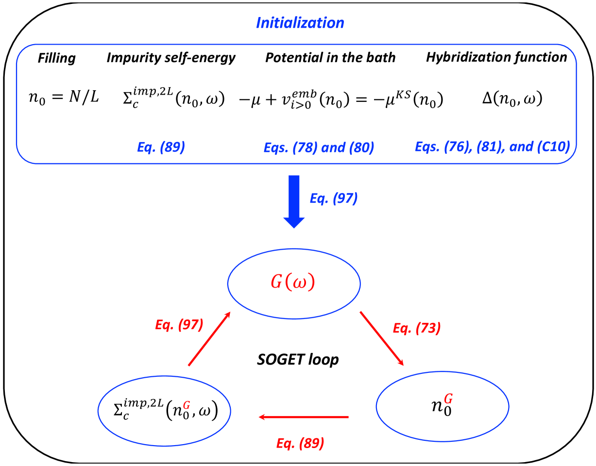
Figure 1: Schematics of the (semi-) self-consistent implementation of SOGET used in this work.

In order to implement SOGET, we had to make a series of approximations which have been discussed in detail in Sec. III. A graphical summary of our implementation is given in Fig. 1. The key steps, in both the initialization and the (semi-) self-consistency cycle of SOGET, are highlighted. Density-functional correlation energies have been modelled at the 2L-BALDA level of approximation (see Sec. III.1). The method has been applied to the 1D Hubbard model with $L=400$ sites and a smearing parameter of $\eta=0.01$. As we use an impurity-interacting self-energy with explicit dependence on the density, calculations are extremely cheap and not limited by the size of the system so that, in practice, any filling can be reproduced. Comparison is made with conventional (KS) BALDA and exact BA results Lieb and Wu (1968); Shiba (1972). For analysis purposes, exact and approximate SOGET spectral functions have been computed for a half-filled 12-site Hubbard ring via an exact diagonalization Lin et al. (1993) with 100 Lanczos iterations and a peak broadening of $\eta=0.05$. In all calculations, we set $t=1$.

V Results and discussion

V.1 Self-consistently converged site occupations

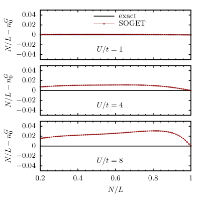
Figure 2: Deviation of the exact filling $N/L$ [$L=400$] from the converged impurity site occupation $n^{G}_{0}$ for different interaction strengths. The self-consistently converged Green’s function and the corresponding site occupation are computed according to Eqs. (97) and (73), respectively.

Ideally, the self-consistently converged impurity Green’s function should restore the exact filling of the physical Hubbard model. Despite the use of approximate density-functional (self-) energies, it turns out to be the case at half-filling (see Fig. 2), as expected from Sec. III.2. In the hole-doped case, however, the converged impurity site occupation deviates from the exact filling. In the weakly correlated regime the error is almost unnoticeable but it becomes more important as we approach the strongly correlated regime. The deviation remains relatively small though, unlike in the standard implementation of SOET Senjean et al. (2018a, b). In the latter case, the computation of a many-body wavefunction allows for unphysical charge transfers between impurity and bath sites. Such excitation processes are favored by the approximations made in the density-functional embedding potential. More precisely, as shown in Ref. Senjean et al. (2018b), the deviation of the converged impurity occupation from the exact filling is controlled by the relative position of the 2L impurity-interacting and BALDA correlation potentials on the impurity site, which actually changes with site occupation. In SOGET, this does not occur as the problem is fully mapped onto the impurity site by using an hybridization function and the BALDA density-functional chemical potential. As shown in Fig. 2, the impurity occupation is systematically lower than the exact filling in all correlation regimes, and the error smoothly vanishes when approaching half-filling, unlike in SOET (see Fig. 7 of Ref. Senjean et al. (2018b)).

V.2 Double occupations and per-site energies

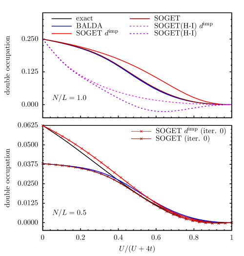
Figure 3: SOGET double occupation computed as a function of the correlation strength at half- (top panel) and quarter-fillings (bottom panel) according to Eqs. (97), (100) and (101). Comparison is made with conventional BALDA and exact BA results (which are equal at half-filling, by construction). Double occupations obtained without density-functional corrections ($d^{\rm imp}$) and/or within the Hubbard-I (H-I) self-energy approximation (at half-filling only) are shown for analysis purposes. Self-consistency effects (which vanish at half-filling) are slightly visible at quarter filling only in the strongly correlated limit [see “iter. 0” curves].

Double occupations obtained with and without density-functional corrections are shown in Fig. 3. They are plotted as functions of $U/(U+4t)$ in order to cover all correlation regimes, from the weakly [$U/(U+4t)\rightarrow 0$] to the strongly correlated one [$U/(U+4t)\rightarrow 1$]. At half-filling, the bare SOGET impurity double-occupation obtained from Eq. (101) is, like in SOET Senjean et al. (2018a, b) or DMET Knizia and Chan (2012), too high. While, in DMET, this issue is solved by increasing the number of impurities, we recover here almost the exact result with a single impurity by adding the appropriate density-functional correction [terms in square brackets on the right-hand side of Eq. (100)]. Interestingly, the improvement is also substantial in SOET Senjean et al. (2018b) but not as impressive as in SOGET. This is due to error cancellations. Indeed, combining our approximate local impurity-interacting Green’s function with the 2L impurity-interacting self-energy leads to an underestimation of the bare impurity double occupation [see the accurate DMRG values labelled as “iBALDA($M$=1)” in Fig. 2 of Ref. Senjean et al. (2018b)]. Consequently, SOGET yields better results than SOET when the 2L-BALDA density-functional correction is applied.

For comparison, we also computed SOGET double occupations obtained by substituting the H-I self-energy for the 2L impurity-interacting one. As shown in the top panel of Fig. 3, in this case, the bare impurity double occupancy is far from the physical one except in both non-interacting and $U/t\rightarrow+\infty$ limits. Due to the absence of the hopping parameter $t$ in the atomic limit, the H-I self-energy overestimates the effect of the Coulomb interaction $U$ and tends to localize the electrons as soon as $U/t$ deviates from zero. The inclusion of a non-local hopping parameter in the 2L approximation apparently mimics the fluctuations between the bath and the impurity and favors the delocalization of electrons. Note that adding density-functional corrections to the bare impurity double occupancy deteriorates the results further when the H-I self-energy is employed. Unphysical negative double occupations are even obtained in intermediate correlation regimes. H-I performs also poorly away from half-filling (not shown).

At quarter-filling, SOGET slightly underestimates the exact double occupation in the strongly correlated regime [i.e. when $U/(U+4t)>0.5$], as shown in the bottom panel of Fig. 3. However, in the weakly correlated regime, SOGET yields wrong double occupations once the density-functional corrections are applied. The error is inherited from BALDA [first term on the right-hand side of Eq. (100)] which, by construction, reproduces the exact BA result only at half-filling. Away from half-filling, the BALDA correlation functional exhibits an unphysical linear variation in $U$ (see Eq. (31) in Ref. Senjean et al. (2018a)) which artificially lowers the double occupation in the $U/t\rightarrow 0$ limit. In this case, the bare impurity double occupation is much more accurate. Per-site energies are shown in Fig. 4. For all fillings and correlation strengths, SOGET yields accurate results and even improves on previous results from SOET Senjean et al. (2018a, b).

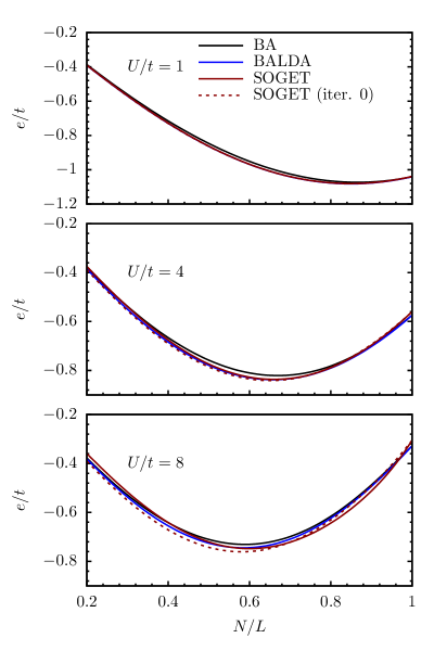
Figure 4: SOGET per-site energy plotted as a function of the filling $N/L$ [$L=400$] according to Eqs. (97) and (99) for different correlation strengths. Comparison is made with conventional BALDA and exact BA results. Results obtained at iteration 0 in Eq. (97) (i.e. when $n^{G}_{0}=N/L$) are also shown [dashed lines] for analysis purposes. SOGET and BALDA curves are almost indistinguishable for $U/t=1$.

Finally, as for the comparison of conventional BALDA with SOGET, both approaches qualitatively exhibit the same performance. In the light of Eqs. (100) and (101), we can conclude that the locality of the self-energy, which was assumed in Eqs. (71) and (89) and is a key approximation in DMFT, is also relevant in SOGET. It also means that the local part of the SOGET Green’s function, which incorporates information about the bath through the hybridization function, can be combined with the self-energy of a simple system like the Anderson dimer and deliver meaningful results.

V.3 Mott–Hubbard transition

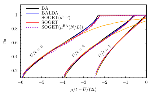
Figure 5: Mott–Hubbard transition explored in SOGET for different correlation strengths. In a first approach we plot, as the filling $N/L$ varies, the self-consistently converged impurity occupation as a function of the BALDA chemical potential $\mu^{\rm BA}(N/L)$ where $L=400$ [dashed curves]. A second approach (simply referred to as SOGET) consists in implementing Eqs.(98) and (102). Results obtained without density-functional corrections to $d^{\rm imp}$ [SOGET($d^{\rm imp}$)] are also shown. Comparison is made with conventional BALDA and exact BA results.

As discussed in detail in Sec. III.4, the BALDA chemical potential is used in SOGET in order to ensure a smooth convergence of the impurity site occupation in all correlation regimes and fillings. Therefore, plotting the occupation as a function of the chemical potential with SOGET and conventional BALDA will give exactly the same result if self-consistency is neglected. In this case, the Mott–Hubbard transition is qualitatively well reproduced (see Fig. 5). This well-known feature of BALDA is due to the derivative discontinuity that the BALDA correlation potential exhibits at half-filling. In order to evaluate the impact of the density-functional approximations made in the impurity-interacting correlation (self-) energy, we first plotted the self-consistently converged occupation with respect to the filling-functional BALDA chemical potential. Results are shown in Fig. 5. As expected from Fig. 2, in the strongly correlated regime, we observe a slight deviation from BALDA.

Another (less straightforward though) way to investigate the transition consists in minimizing the SOGET per-site grand canonical energy according to Eqs. (98) and (102). As clearly seen from Fig. 5, we obtain similar results to BALDA. A slight deviation appears as the correlation strength increases but the plateau is relatively well reproduced. Most importantly, if we remove the density-functional corrections to the “bare” impurity double occupation, the Mott–Hubbard transition disappears. The results look then quite similar to those obtained in single-site DMET. It clearly shows that BALDA (or, more precisely, the derivative discontinuity that its correlation potential exhibits at half-filling) plays a crucial role in the description of the transition in the single-impurity formulation of SOGET, as expected from Sec. II.3.3.

Note that, once the density-functional corrections to the double impurity site occupation [see Eq. (100)] are included, we essentially obtain the right answer through error cancellations. If we turn to the exact Green’s function’s expression in Eq. (II.3.3) and the discussion that follows, the shift in chemical potential observed at half-filling should, on the impurity site, originate from the impurity-interacting self-energy, while the derivative discontinuities in the fully- and impurity-interacting correlation potentials should cancel each other. These features should of course be reflected in the per-site energy [see the exact expression given in Eqs. (24) and (51)-(52)] or, more precisely, in its density-functional derivative from which the chemical potential can in principle be extracted. Unlike in the exact theory, the 2L approximate impurity-interacting correlation potential does not exhibit a derivative discontinuity at $n_{0}=1$ for finite $U/t$ values. This is due to the fact that the two-electron Anderson dimer it originates from is a closed system Senjean et al. (2017, 2018b). One could make the same comment about the 2L impurity-interacting density-functional self-energy. Finally, no discontinuity will appear in our approximate (semi-) self-consistently converged Green’s function as it is determined from the (continuous) KS chemical potential [see Eq. (97)]. As a result, in our simplified implementation of SOGET depicted in Eqs. (97) and (98)-(102), the BALDA correlation functional [see the first term on the right-hand side of Eq. (100)] is responsible for the functional derivative discontinuity which makes the Mott–Hubbard transition possible. This is also the reason why BALDA and SOGET exhibit exactly the same gap.

V.4 Spectral function

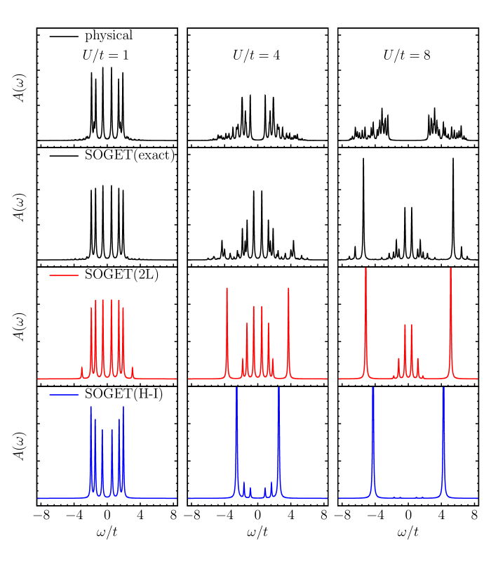
Figure 6: Spectral functions $A(\omega)=-(1/\pi)\mathrm{Im}\,\left[G\left(\omega\right)\right]$ computed on the impurity site of a half-filled 12-site ring ($\mu=U/2$) for various interaction strengths and Green’s functions. From top to bottom: physical Hubbard model, exact SOGET, SOGET with 2L and H-I density-functional self-energies, respectively. See Sec. IV for further details.

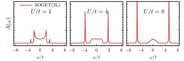
Figure 7: SOGET spectral function $A(\omega)=-(1/\pi)\mathrm{Im}\,\left[G\left(\omega\right)\right]$ obtained for a half-filled 400-site ring and various interaction strengths. The impurity-interacting Green’s function $G\left(\omega\right)$ has been computed according to Eq. (97) with the 2L density-functional correlation self-energy.

Let us now focus on the local Green’s function that is computed in SOGET. For analysis purposes, we first generated the corresponding spectral function for a half-filled 12-site ring. Results are shown in Fig. 6 and compared with exact and other approximate spectral functions. The exact physical and impurity-interacting spectral functions differ substantially as the correlation strength increases. Indeed, in exact SOET or SOGET, the impurity-interacting system is expected to reproduce the physical impurity site occupation only. Like in KS-DFT, one should not expect the physical local Green’s function or its spectral function to be reproduced. The opening of the gap that the physical Green’s function exhibits cannot be seen in the impurity-interacting system simply because, in this case, the interactions in the bath have been replaced by a local potential. As discussed in detail in Sec. II.3.3, the fact that the latter potential exhibits a derivative discontinuity in the bath plays a crucial role in the (effective) description of the physical gap opening. The gap will open when plotting the impurity site occupation as a function of $\mu$ even though the (impurity-interacting and bath-non-interacting) spectral gap is closed.

Interestingly, 2L-BALDA reproduces very well many features of the exact impurity-interacting spectral function, especially in weak and strong correlation regimes. Some features like satellites are missing though, due to the (oversimplified) Anderson-dimer-based 2L self-energy we use. The spectral function obtained at the same level of approximation for the half-filled 400-site ring is shown in Fig. 7. Some features of the 4-site DMET and cluster DMFT spectral functions shown in Fig. 1 of Ref. Booth and Chan (2015) are recovered but, most importantly, the latter exhibit an open gap while our single-impurity SOGET spectral function does not. Once again, this is not in contradiction with the gap opening that SOGET exhibits in Fig. 5, simply because the physical and impurity-interacting spectral gaps are not expected to match, even in the exact theory (see Sec. II.3.3). It would be interesting to see how the spectral gap of the impurity-interacting system evolves with the number of impurities. This would require new developments that are left for future work.

Finally, if we return to the simpler 12-site model of Fig. 6, the SOGET spectral function generated from the Hubbard-I self-energy is much closer to the exact physical one than the exact impurity-interacting one. In a theory like DMFT where the local Green’s function is the quantity to be reproduced by an impurity-interacting system, Hubbard-I is a sound approximation. However, in the light of the double occupation plots shown in Fig. 3, the 2L self-energy seems to be a better choice in SOGET.

VI Conclusions and perspectives

A novel and in-principle-exact reformulation of SOET (referred to as SOGET) in terms of Green’s functions has been derived. Once the local self-energy approximation is made, SOGET becomes formally very similar to DMFT. However, unlike in DMFT, self-consistency occurs through the density, which is the basic variable in SOGET. In other words, the impurity-interacting self-energy is treated as a functional of the (ground-state) density. A simple density-functional approximation based on the Anderson dimer has been successfully applied to the 1D Hubbard model. While previous implementations of SOET required the computation of a correlated many-body wavefunction for the full impurity-interacting system, SOGET remaps the impurity correlation problem onto a density-functional dimer. The drastic reduction in computational cost allowed us to approach the thermodynamic limit and to model the density-driven Mott–Hubbard transition (in 1D). Interestingly, thanks to error cancellations, SOGET gave, at half-filling, even more accurate per-site energies and double occupations than SOET. Spectral functions have also been analyzed. Unlike in DMFT, the proper description of gap openings in single-impurity SOGET relies on derivative discontinuities in correlation potentials, like in DFT. The BALDA functional, which was used for modelling the bath, contains such a discontinuity, by construction. The Mott–Hubbard transition is lost if the latter is neglected in the SOGET energy expression.

The single-impurity formulation of SOGET presented in this work should be applicable to the two- and three-dimensional Hubbard model. One key ingredient, that was missing in the literature until very recently, is the extension of the one-dimensional BALDA functional to higher dimensions Vilela et al. (2019). In order to establish clearer connections between SOGET and DMFT, the infinite-dimension limit of SOGET should also be explored. Work is currently in progress in these directions. Note also that, like DFT, SOGET can formally be extended to time-dependent regimes and finite temperatures, thus giving in principle access to dynamical properties. The exploration of such extensions is left for future work.

The applicability of SOGET to a wider range of strongly correlated systems (including ab initio ones) relies on the development of density-functional approximations for the (static) impurity-interacting correlation functional and the (dynamical) impurity-interacting correlation self-energy. The impurity-interacting Sham–Schlüter Eq. (II.2.1) is a formally-exact constraint which might be used to develop better approximations to the embedding potential, provided that we can obtain better density-functional self-energies. While an explicit density-dependence (like in the 2L Anderson model) is difficult, if not impossible, to reach for any system, designing an impurity-interacting self-energy which is an implicit functional of the density is computationally more demanding but still affordable, in particular if the size of the system to be described with Green’s functions can be substantially reduced. It would then become possible, in practice, to extend SOGET to multiple impurities, like in SOET Senjean et al. (2018b). Starting from the SOET self-consistent Eq. (20), a simple solution would consist in applying the Schmidt decomposition to the full impurity-interacting system and adding dynamical fluctuation corrections, in the spirit of Refs. Senjean (2019) and Fertitta and Booth (2018). The latter are expected to be relatively small due to the density-functional description of the SOET bath. As the number of impurities increases, we expect the description of derivative discontinuities in the bath to be less critical, thus making the accuracy of the method less density-functional-dependent. In order to turn SOGET into a practical computational method, one should obviously find the right balance in terms of computational cost (in solving the impurity-interacting problem) versus feasibility in designing good bath correlation functionals.

Let us mention that an alternative approach, where no many-body wavefunction for the full SOET system would be needed, would consist in applying a Householder transformation to the one-electron reduced density matrix (or, eventually, the frequency-dependent Green’s function) in order to map the properties of the impurity-interacting system of SOET onto a (much smaller and possibly open) cluster, in the spirit of DMET. Work is currently in progress in this direction.

Turning finally to ab initio extensions of SOGET, various strategies that recently appeared in the literature might be considered. The first one is the Requist–Gross interacting lattice model that is rigorously coupled to DFT Requist and Gross (2019). Another one is DFT with domain separation, as proposed by Mosquera et al. Mosquera et al. (2019), which can be seen as an ab initio generalization of SOET. Substituting a Green’s function treatment of a given domain for the many-body wavefunction one would provide an ab initio version of SOGET. The latter would in principle be free from double counting, unlike DMFT+DFT Kotliar et al. (2006).

VII Acknowledgments

L. M. and E. F. would like to thank B. Senjean for fruitful discussions and for providing his implementation of the impurity-interacting correlation potential and energy for the Anderson dimer. They also thank M. Tsuchiizu for his useful advices concerning the formalism of Green’s functions. This work was funded by the Ecole Doctorale des Sciences Chimiques 222 (Strasbourg).

Appendix A Green’s function of the Hubbard dimer

In this section, we calculate the exact Green’s function of the singlet ground-state of the asymmetric two-electron Hubbard dimer. We use the following Hamiltonian,

$$\hat{H}=-t\sum_{\sigma}(\hat{a}^{\dagger}_{0\sigma}\hat{a}_{1\sigma}+\hat{a}^{\dagger}_{1\sigma}\hat{a}_{0\sigma})+\sum^{1}_{i=0}U_{i}\hat{n}_{i\uparrow}\hat{n}_{i\downarrow}+\sum^{1}_{i=0}v_{i}\hat{n}_{i}\,.$$

For such as system, the matrix elements of the frequency-dependent retarded Green’s function in the Lehmann representation read

$$G_{i\sigma,j\sigma^{\prime}}(\omega)=\sum_{a=0}^{1}\dfrac{L_{i\sigma,j\sigma^{\prime}}^{a}}{\omega+I_{a}+{\rm i}\eta}+\sum_{b=0}^{1}\dfrac{M_{i\sigma,j\sigma^{\prime}}^{b}}{\omega+A_{b}+{\rm i}\eta}$$

(104)

where

$$L_{i\sigma,j\sigma^{\prime}}^{a}=f_{i\sigma,a}f_{j\sigma^{\prime},a}^{\star}$$ (105)

and

$$M_{i\sigma,j\sigma^{\prime}}^{b}=f_{i\sigma,b}f_{j\sigma^{\prime},b}^{\star}$$ (106)

are the spectral weights and

$$I_{a}=E_{a}^{N=1}-E_{0}^{N=2}$$ (107)

and

$$A_{b}=E_{0}^{N=2}-E_{b}^{N=3}$$ (108)

are the poles of the Green’s function. The spectral weights are calculated via the Dyson orbitals defined as follows

$$f_{i\sigma,a}=\langle\Psi_{0}^{N=2}|\hat{a}_{i\sigma}^{\dagger}|\Psi_{a}^{N=1}\rangle$$ (109)

and

$$f_{i\sigma,b}=\langle\Psi_{0}^{N=2}|\hat{a}_{i\sigma}|\Psi_{b}^{N=3}\rangle\,.$$ (110)

The summations run over the full space of one- and three-electron states of the system. The poles and Dyson orbitals can all be calculated analytically in the case of the Hubbard dimer. First, we solve the trivial one- and three-electron Hubbard dimers. Note that, in the absence of a magnetic field, the Hamiltonians for the two doublets ($s=+1/2$ and $s=-1/2$) are the same. The Hilbert space in the site basis for the one-electron Hubbard dimer reads

$$|\phi_{1}\rangle = \hat{a}_{0\uparrow}^{\dagger}|{\rm vac}\rangle$$

$$|\phi_{2}\rangle = \hat{a}_{1\uparrow}^{\dagger}|{\rm vac}\rangle$$

$$|\phi_{3}\rangle = \hat{a}_{0\downarrow}^{\dagger}|{\rm vac}\rangle$$

$$|\phi_{4}\rangle = \hat{a}_{1\downarrow}^{\dagger}|{\rm vac}\rangle\,$$ (111)

and the Hamiltonian for both doublets ($s=+1/2$ and $s=-1/2$) becomes

$$\mathbf{H}^{N=1}=\begin{bmatrix}\begin{array}[]{cc}v_{0}&-t\\ -t&v_{1}\\ \end{array}\end{bmatrix}\,.$$ (112)

The eigenvalues and the corresponding eigenvectors of the one-electron ($N=1$) Hubbard dimer read

$$E_{0}^{N=1} = \dfrac{1}{2}\Big{[}v_{1}+v_{0}-\sqrt{4t^{2}+\Delta v^{2}}\Big{]}$$

$$E_{1}^{N=1} = \dfrac{1}{2}\Big{[}v_{1}+v_{0}+\sqrt{4t^{2}+\Delta v^{2}}\Big{]}$$

where $\Delta v=v_{1}-v_{0}$, and

$$c_{0k}^{N=1}=\cos\big(\tan^{-1}(\alpha_{k})\big{missing})$$

$$c_{1k}^{N=1}=\sin\big(\tan^{-1}(\alpha_{k})\big{missing})$$ (114)

with $\alpha_{k}=(v_{0}-E^{N=1}_{k})/t$. The wavefunctions of the one-electron Hubbard dimer are expressed as follows,

$$|\Psi_{0}^{N=1}\rangle=c_{00}^{N=1}|\phi_{1}\rangle+c_{10}^{N=1}|\phi_{2}\rangle$$

$$|\Psi_{1}^{N=1}\rangle=c_{01}^{N=1}|\phi_{3}\rangle+c_{11}^{N=1}|\phi_{4}\rangle$$ (115)

$$|\Psi_{2}^{N=1}\rangle=c_{00}^{N=1}|\phi_{1}\rangle+c_{10}^{N=1}|\phi_{2}\rangle$$

$$|\Psi_{3}^{N=1}\rangle=c_{01}^{N=1}|\phi_{3}\rangle+c_{11}^{N=1}|\phi_{4}\rangle$$ (116)

The Hilbert space in the site basis for the three-electron ($N=3$) Hubbard dimer reads

$$|\phi_{1}\rangle = \hat{a}_{0\uparrow}^{\dagger}\hat{a}_{0\downarrow}^{\dagger}\hat{a}_{1\downarrow}^{\dagger}|{\rm vac}\rangle$$

$$|\phi_{2}\rangle = \hat{a}_{1\uparrow}^{\dagger}\hat{a}_{0\uparrow}^{\dagger}\hat{a}_{1\downarrow}^{\dagger}|{\rm vac}\rangle$$

$$|\phi_{3}\rangle = \hat{a}_{0\uparrow}^{\dagger}\hat{a}_{0\downarrow}^{\dagger}\hat{a}_{1\downarrow}^{\dagger}|{\rm vac}\rangle$$

$$|\phi_{4}\rangle = \hat{a}_{1\uparrow}^{\dagger}\hat{a}_{0\downarrow}^{\dagger}\hat{a}_{1\downarrow}^{\dagger}|{\rm vac}\rangle$$ (117)

and the Hamiltonian for both doublets ($s=+1/2$ and $s=-1/2$) becomes

$$\mathbf{H}^{N=3}=\begin{bmatrix}\begin{array}[]{cc}2v_{0}+v_{1}+U_{0}&-t\\ -t&v_{0}+2v_{1}+U_{1}\\ \end{array}\end{bmatrix}\,.$$ (118)

The eigenvalues and the corresponding eigenvectors of the three-electron Hubbard dimer read

$$E_{0}^{N=3} = \frac{1}{2}\Bigg{[}U_{0}+U_{1}+3(v_{0}+v_{1})$$

$$-\sqrt{4t^{2}+\big{(}\Delta v+\Delta U\big{)}^{2}}\Bigg{]}$$

$$E_{1}^{N=3} = \frac{1}{2}\Bigg{[}U_{0}+U_{1}+3(v_{0}+v_{1})$$ (119)

$$+\sqrt{4t^{2}+\big{(}\Delta v+\Delta U\big{)}^{2}}\Bigg{]}$$

where $\Delta U=U_{1}-U_{0}$, and

$$c_{0k}^{N=3}=\cos\big(\tan^{-1}(\beta_{k})\big{missing})$$

$$c_{1k}^{N=3}=\sin\big(\tan^{-1}(\beta_{k})\big{missing})$$ (120)

with $\beta_{k}=(2v_{0}+v_{1}+U_{0}-E_{k})/t$. The wavefunctions of the three-electron Hubbard dimer are expressed as follows,

$$|\Psi_{0}^{N=3}\rangle=c_{00}^{N=3}|\phi_{1}\rangle+c_{10}^{N=3}|\phi_{2}\rangle$$

$$|\Psi_{1}^{N=3}\rangle=c_{01}^{N=3}|\phi_{3}\rangle+c_{11}^{N=3}|\phi_{4}\rangle$$ (121)

$$|\Psi_{2}^{N=3}\rangle=c_{00}^{N=3}|\phi_{1}\rangle+c_{10}^{N=3}|\phi_{2}\rangle$$

$$|\Psi_{3}^{N=3}\rangle=c_{01}^{N=3}|\phi_{3}\rangle+c_{11}^{N=3}|\phi_{4}\rangle$$ (122)

Then, we calculate the singlet ground state energy and wavefunction of the two-electron $(N=2)$ Hubbard dimer. We use the following Hilbert space,

$$|\phi_{1}\rangle = \hat{a}_{0\uparrow}^{\dagger}\hat{a}_{0\downarrow}^{\dagger}|{\rm vac}\rangle$$

$$|\phi_{2}\rangle = \hat{a}_{1\uparrow}^{\dagger}\hat{a}_{1\downarrow}^{\dagger}|{\rm vac}\rangle$$

$$|\phi_{3}\rangle = \frac{1}{\sqrt{2}}(\hat{a}_{0\uparrow}^{\dagger}\hat{a}_{1\downarrow}^{\dagger}+\hat{a}_{1\uparrow}^{\dagger}\hat{a}_{0\downarrow}^{\dagger})|{\rm vac}\rangle$$ (123)

The two-electron Hamiltonian then reads

$$\mathbf{H}^{N=2}=\begin{bmatrix}\begin{array}[]{cccc}U_{0}+2v_{0}&0&-\sqrt{2}t\\ 0&U_{1}+2v_{1}&-\sqrt{2}t\\ -\sqrt{2}t&-\sqrt{2}t&v_{0}+v_{1}\\ \end{array}\end{bmatrix}\,.$$ (124)

The ground-state eigenvalues a solution of the cubic secular equation of the Hamiltonian and is written as follows,

$$E_{0}^{N=2}=2\sqrt{-Q}\cos\Big(\frac{\Theta+2\pi}{3}\Big{missing})+\frac{U_{0}+U_{1}}{3}+v_{0}+v_{1}$$

(125)

where

$$\Theta=\cos^{-1}\Big{(}\frac{R}{\sqrt{-Q^{3}}}\Big{)}\,,$$ (126)

$$R=\dfrac{9a_{2}a_{1}-27a_{0}-2a_{2}^{3}}{54}$$ (127)

and

$$Q=\dfrac{3a_{1}-a_{2}^{2}}{9}$$ (128)

with

$$a_{0} = (v_{0}+v_{1})(4t^{2}-U_{0}U_{1}-4v_{0}v_{1})$$

$$+ 2(U_{0}+U_{1})(t^{2}-v_{0}v_{1})-2(U_{0}v_{1}^{2}+U_{1}v_{0}^{2})\,,$$

$$a_{1} = U_{0}U_{1}+8v_{0}v_{1}-4t^{2}+2(v_{0}^{2}+v_{1}^{2})$$ (130)

$$+ U_{0}(v_{0}+3v_{1})+U_{1}(v_{1}+3v_{0})\,,$$

and

$$a_{2}=-(U_{0}+U_{1})-3(v_{0}+v_{1})\,.$$ (131)

The two-electron wavefunction of the Hubbard dimer reads

$$\Psi_{0}^{N=2}=c_{1}^{N=2}|\phi_{1}\rangle+c_{2}^{N=2}|\phi_{2}\rangle+c_{3}^{N=2}|\phi_{3}\rangle$$ (132)

where

$$c_{1}^{N=2}=\frac{A}{\sqrt{A^{2}+B^{2}+2A^{2}B^{2}/(4t^{2})}}$$

$$c_{2}^{N=2}=\frac{B}{\sqrt{A^{2}+B^{2}+2A^{2}B^{2}/(4t^{2})}}$$

$$c_{3}^{N=2}=\frac{\sqrt{2}\frac{AB}{2t}}{\sqrt{A^{2}+B^{2}+2A^{2}B^{2}/(4t^{2})}}$$ (133)

with

$$A = U_{1}+2v_{1}-E_{0}^{N=2}$$

$$B = U_{0}+2v_{0}-E_{0}^{N=2}\,.$$ (134)

With Eqs. (116), (122) and 132), we calculate the Dyson orbitals,

$$f_{0\sigma,a}=-\dfrac{A\cos(\tan^{-1}\alpha_{a})+\frac{AB}{2t}\sin(\tan^{-1}\alpha_{a})}{\sqrt{A^{2}+B^{2}+2A^{2}B^{2}/(4t^{2})}}$$

$$f_{1\sigma,a}=-\dfrac{B\sin(\tan^{-1}\alpha_{a})+\frac{AB}{2t}\cos(\tan^{-1}\alpha_{a})}{\sqrt{A^{2}+B^{2}+2A^{2}B^{2}/(4t^{2})}}$$

$$f_{0\sigma,b}=\dfrac{B\sin(\tan^{-1}\beta_{b})+\frac{AB}{2t}\cos(\tan^{-1}\beta_{b})}{\sqrt{A^{2}+B^{2}+2A^{2}B^{2}/(4t^{2})}}$$

$$f_{1\sigma,b}=-\dfrac{A\cos(\tan^{-1}\beta_{b})+\frac{AB}{2t}\sin(\tan^{-1}\beta_{b})}{\sqrt{A^{2}+B^{2}+2A^{2}B^{2}/(4t^{2})}}\,.$$

The poles are calculated with Eqs. (LABEL:eq:app_energy_one), (119) and (125). Now, we possess all the quantities we need in order to calculate the Green’s function [Eq. 104]. The non-interacting Green’s function is easily calculated by setting $U_{0}=U_{1}=0$,

$$G^{0}_{0\sigma,0\sigma^{\prime}}(\omega) = \dfrac{\delta_{\sigma\sigma^{\prime}}}{2}\bigg{[}\dfrac{1+\sin(\tan^{-1}\frac{\Delta v}{2t})}{\omega-(v_{0}+v_{1}-\sqrt{4t^{2}+\Delta v^{2}})/2+{\rm i}\eta}$$

$$+ \dfrac{1-\sin(\tan^{-1}\frac{\Delta v}{2t})}{\omega-(v_{0}+v_{1}+\sqrt{4t^{2}+\Delta v^{2}})/2+{\rm i}\eta}\bigg{]}\,,$$

$$G^{0}_{1\sigma,1\sigma^{\prime}}(\omega) = \dfrac{\delta_{\sigma\sigma^{\prime}}}{2}\bigg{[}\dfrac{1-\sin(\tan^{-1}\frac{\Delta v}{2t})}{\omega-(v_{0}+v_{1}-\sqrt{4t^{2}+\Delta v^{2}})/2+{\rm i}\eta}$$

$$+ \dfrac{1+\sin(\tan^{-1}\frac{\Delta v}{2t})}{\omega-(v_{0}+v_{1}+\sqrt{4t^{2}+\Delta v^{2}})/2+{\rm i}\eta}\bigg{]}\,,$$

$$G^{0}_{0\sigma,1\sigma^{\prime}}(\omega) = \dfrac{\delta_{\sigma\sigma^{\prime}}}{2}\bigg{[}\dfrac{\cos(\tan^{-1}\frac{\Delta v}{2t})}{\omega-(v_{0}+v_{1}-\sqrt{4t^{2}+\Delta v^{2}})/2+{\rm i}\eta}$$

$$- \dfrac{\cos(\tan^{-1}\frac{\Delta v}{2t})}{\omega-(v_{0}+v_{1}+\sqrt{4t^{2}+\Delta v^{2}})/2+{\rm i}\eta}\bigg{]}$$

In the non-interacting KS Green’s function of the asymmetric dimer $\mathbf{G}^{\rm KS,2L}({n}_{0},\omega)$, we choose the following on-site potentials

$$v_{0}=-\Delta v^{\rm KS}(n_{0})=-\frac{2t(n_{0}-1)}{\sqrt{n_{0}(2-n_{0})}}$$

$$v_{1}=0\,.$$ (137)

The interacting impurity Green’s function of the asymmetric Anderson dimer $\mathbf{G}^{\rm imp,2L}({n}_{0},\omega)$ as a functional of the site occupation is obtained by switching off the interaction on site 1 ( $U_{0}=U$ and $U_{1}=0$) and setting

$$v_{0}=-\Delta v^{\rm emb}(n_{0})=-\Delta v^{\rm KS}(n_{0})+\Delta v_{\rm Hxc}^{\rm imp}(U,n_{0})$$

$$v_{1}=0\,,$$ (138)

where

$$\Delta v_{\rm Hxc}^{\rm imp}(U,n_{0})=-\frac{U}{2}n_{0}-\frac{\partial E_{\rm c}^{\rm 2L}(U/2,n_{0})}{\partial n_{0}}.$$ (139)

The two-level impurity correlation self-energy [Eq. (89)] is then obtained by inverting the KS and interacting Anderson Green’s functions of the impurity site and subtracting the impurity potential $\Delta v_{\rm Hxc}^{\rm imp}(U,n_{0})$,

$$\Sigma_{\rm c}^{\rm imp,2L}({n}_{0},\omega) = \frac{1}{G_{0\sigma,0\sigma}^{\rm KS,2L}(\omega,n_{0})}-\frac{1}{G_{0\sigma,0\sigma}^{\rm imp,2L}(\omega,n_{0})}$$ (140)

$$-\Delta v_{\rm Hxc}^{\rm imp}(U,n_{0})\,.$$

The formulas to calculate the exact impurity potential $\Delta v_{\rm Hxc}^{\rm imp}(U,n_{0})$ for the asymmetric Hubbard dimer have been derived in Refs. Carrascal et al. (2015, 2016); Senjean et al. (2018b). In the symmetric Anderson dimer ($v_{0}=-U/2$, $v_{1}=0$) and $n=1$, there is an analytic expression for the exact impurity Green’s function and self-energy Lange (1998),

$$G_{00}^{\rm imp}(\omega) = \dfrac{1}{4}\bigg{[}\dfrac{1-\frac{U^{2}-32t^{2}}{\sqrt{(U^{2}+64t^{2})(U^{2}+16t^{2})}}}{\omega-(\sqrt{U^{2}+64t^{2}}-\sqrt{U^{2}+16t^{2}})/4+{\rm i}\eta}$$

$$+ \dfrac{1+\frac{U^{2}-32t^{2}}{\sqrt{(U^{2}+64t^{2})(U^{2}+16t^{2})}}}{\omega-(\sqrt{U^{2}+64t^{2}}+\sqrt{U^{2}+16t^{2}})/4+{\rm i}\eta}$$

$$+ \dfrac{1-\frac{U^{2}-32t^{2}}{\sqrt{(U^{2}+64t^{2})(U^{2}+16t^{2})}}}{\omega+(\sqrt{U^{2}+64t^{2}}-\sqrt{U^{2}+16t^{2}})/4+{\rm i}\eta}$$

$$+ \dfrac{1+\frac{U^{2}-32t^{2}}{\sqrt{(U^{2}+64t^{2})(U^{2}+16t^{2})}}}{\omega+(\sqrt{U^{2}+64t^{2}}+\sqrt{U^{2}+16t^{2}})/4+{\rm i}\eta}\bigg{]}\,,$$

$$\Sigma_{{\rm Hxc}}^{\rm imp}(n_{0}=1,\omega)=\dfrac{U}{2}+\dfrac{1}{2}\bigg{[}\dfrac{(\frac{U}{2})^{2}}{\omega-3t+{\rm i}\eta}+\dfrac{(\frac{U}{2})^{2}}{\omega+3t+{\rm i}\eta}\bigg{]}\,.$$

Appendix B Hybridization function

The approximate interaction-free Green’s function on the impurity site $\mathcal{G}^{\rm imp}\left({n}_{0},\omega\right)$ can be seen as a density-functional Weiss field. According to Eqs. (48) and (LABEL:eq:approx_embedding_potential), it can be expressed as follows:

$$\mathcal{G}^{\rm imp}\left({n}_{0},\omega\right)=\mathcal{G}_{0\sigma,0\sigma}^{\rm imp}\left({n}_{0},\omega\right),$$

where

$$\left[\mathbfcal{G}^{\rm imp}\left({n}_{0},\omega\right)\right]^{-1}=\left(\omega+\mu+{\rm i}\eta\right)\mathbf{I}-\mathbf{t}-\mathbf{v}^{\rm emb}(n_{0}),$$

and

$$v^{\rm emb}_{0}(n_{0}) = \dfrac{\partial e_{\rm c}^{\rm BA}(n_{0})}{\partial n_{0}}-\dfrac{\partial E^{\rm imp}_{\rm c}(n_{0})}{\partial n_{0}},$$

$$v^{\rm emb}_{i}(n_{0}) \overset{i>0}{=} \dfrac{U}{2}n_{0}+\dfrac{\partial e_{\rm c}^{\rm BA}(n_{0})}{\partial n_{0}}.$$ (145)

By diagonalizing the interaction-free Hamiltonian in the bath,

$$\hat{T}+\sum_{i}v^{\rm emb}_{i}(n_{0})\hat{n}_{i}=v^{\rm emb}_{0}(n_{0})\hat{n}_{0}$$

$$+\sum^{\rm bath}_{k}\sum_{\sigma}\varepsilon_{k}(n_{0})\hat{a}^{\dagger}_{k\sigma}\hat{a}_{k\sigma}$$

$$+\sum^{\rm bath}_{k}\sum_{\sigma}\Big{(}V_{0k}\hat{a}^{\dagger}_{0\sigma}\hat{a}_{k\sigma}+V^{*}_{0k}\hat{a}^{\dagger}_{k\sigma}\hat{a}_{0\sigma}\Big{)},$$ (146)

we can rewrite Eq. (B) as follows:

$$\left[\mathbfcal{G}^{\rm imp}\left({n}_{0},\omega\right)\right]^{-1}=\left[\mathbfcal{G}^{\rm bath}\left({n}_{0},\omega\right)\right]^{-1}-\mathbf{V},$$ (147)

or, equivalently,

$$\mathbfcal{G}^{\rm imp}\left({n}_{0},\omega\right) = \mathbfcal{G}^{\rm bath}\left({n}_{0},\omega\right)$$ (148)

$$+\mathbfcal{G}^{\rm bath}\left({n}_{0},\omega\right)\mathbf{V}\mathbfcal{G}^{\rm imp}\left({n}_{0},\omega\right),$$

where the matrix elements of $\mathbf{V}$ are

$$V_{0\sigma,0\sigma^{\prime}} = 0,$$

$$V_{0\sigma,k\sigma^{\prime}} = \delta_{\sigma\sigma^{\prime}}V_{0k},$$

$$V_{k\sigma,0\sigma^{\prime}} = \delta_{\sigma\sigma^{\prime}}V^{*}_{0k}$$

$$V_{k\sigma,k^{\prime}\sigma^{\prime}} = 0$$ (149)

and

$$\mathcal{G}^{\rm bath}_{0\sigma,0\sigma^{\prime}}\left({n}_{0},\omega\right) = \dfrac{\delta_{\sigma\sigma^{\prime}}}{\omega+\mu+{\rm i}\eta-v^{\rm emb}_{0}(n_{0})},$$

$$\mathcal{G}^{\rm bath}_{0\sigma,k\sigma^{\prime}}\left({n}_{0},\omega\right) = \mathcal{G}^{\rm bath}_{k\sigma,0\sigma^{\prime}}\left({n}_{0},\omega\right)=0,$$

$$\mathcal{G}^{\rm bath}_{k\sigma,k^{\prime}\sigma^{\prime}}\left({n}_{0},\omega\right) = \dfrac{\delta_{kk^{\prime}}\delta_{\sigma\sigma^{\prime}}}{\omega+\mu+{\rm i}\eta-\varepsilon_{k}(n_{0})}.$$ (150)

Since, according to Eq. (148),

$$\mathcal{G}^{\rm imp}\left({n}_{0},\omega\right)=\mathcal{G}^{\rm bath}_{0\sigma,0\sigma}\left({n}_{0},\omega\right)$$

$$+\mathcal{G}^{\rm bath}_{0\sigma,0\sigma}\left({n}_{0},\omega\right)\sum_{k}V_{0k}\mathcal{G}_{k\sigma,0\sigma}^{\rm imp}\left({n}_{0},\omega\right),$$ (151)

and

$$\mathcal{G}_{k\sigma,0\sigma}^{\rm imp}\left({n}_{0},\omega\right)=\mathcal{G}^{\rm bath}_{k\sigma,k\sigma}\left({n}_{0},\omega\right)V^{*}_{0k}\mathcal{G}^{\rm imp}\left({n}_{0},\omega\right),$$ (152)

we finally obtain

$$\mathcal{G}^{\rm imp}\left({n}_{0},\omega\right)=\mathcal{G}^{\rm bath}_{0\sigma,0\sigma}\left({n}_{0},\omega\right)$$

$$+\mathcal{G}^{\rm bath}_{0\sigma,0\sigma}\left({n}_{0},\omega\right)\left(\sum_{k}\left|V_{0k}\right|^{2}\mathcal{G}^{\rm bath}_{k\sigma,k\sigma}\left({n}_{0},\omega\right)\right)\mathcal{G}^{\rm imp}\left({n}_{0},\omega\right),$$

thus leading to the expression in Eq. (74) where $\Delta(n_{0},\omega)=\sum_{k}\left|V_{0k}\right|^{2}\mathcal{G}^{\rm bath}_{k\sigma,k\sigma}\left({n}_{0},\omega\right)$.

Appendix C Diagonalization of the interaction-free Hamiltonian in the bath

We divide the non-interacting Hamiltonian into a single impurity and a bath,

$$\mathbf{H}_{0}=\begin{bmatrix}\begin{array}[]{ll}v_{0}^{\rm emb}(n_{0})&\mathbf{h}_{\rm 0k}\\ \mathbf{h}_{\rm k0}^{\dagger}&\mathbf{H}_{\rm kk}\end{array}\end{bmatrix}-\mu\mathbf{I}\,.$$ (154)

The block matrix $\mathbf{H}_{\rm kk}$ describes a non-interacting chain connected to a single impurity on both ends. The part $\mathbf{h}_{\rm 0k}$ ($\mathbf{h}_{\rm k0}^{\dagger}$) contains the connection between the impurity and a non-interacting chain through the hopping parameter. We define a unitary transformation that only diagonalizes the bath,

$$\mathbf{U}=\begin{bmatrix}\begin{array}[]{ll}1&\mathbf{0}\\ \mathbf{0}&\mathbf{C}\end{array}\end{bmatrix}$$ (155)

where $\mathbf{C}$ contains the eigenvectors of the bath. The transformed Hamiltonian

$$\mathbf{U}^{\dagger}\mathbf{H}_{0}\mathbf{U}=\begin{bmatrix}\begin{array}[]{ll}v_{0}^{\rm emb}(n_{0})&\mathbf{V}\\ \mathbf{V}^{\dagger}&\mathbf{E}\end{array}\end{bmatrix}=\mathbf{H}_{0}^{\rm And}$$ (156)

is the non-interacting Anderson model, where $\mathbf{V}=\mathbf{h}_{\rm 0k}\mathbf{C}$ are bath-impurity couplings and $\mathbf{E}=\mathbf{C}^{\dagger}\mathbf{H}_{\rm kk}\mathbf{C}$ is a diagonal matrix containing the eigenvalues [ $\varepsilon_{k}(n_{0})$] of the bath orbitals. The non-interacting Green’s function is obtained by solving a set of linear equations:

$$\big{[}(\omega+{\rm i}\eta+\mu)\mathbf{I}-\mathbf{H}_{0}^{\rm And}\big{]}\bm{\mathcal{G}}^{\rm imp}(n_{0},\omega)=\mathbf{I}$$ (157)

In the case of a single impurity, the expressions for the non-interacting Green’s function are obtained straightforwardly:

$$\bm{\mathcal{G}}^{\rm imp}_{00}(\omega,n_{0})=\dfrac{1}{\omega+\mu+{\rm i}\eta-v_{0}^{\rm emb}(n_{0})-\Delta(n_{0},\omega)}$$ (158)

where

$$\Delta(\omega,n_{0})=\sum_{k=1}\frac{|V_{0k}|^{2}}{\omega+\mu+{\rm i}\eta-\varepsilon_{k}(n_{0})}\,.$$ (159)

For a periodic one-dimensional model with $L$ sites, NN hopping $t$ and constant on-site potential $v_{i>0}^{\rm emb}(n_{0})$ in the bath, we obtain the following analytical expressions for $\varepsilon_{k}(n_{0})$ and the matrix elements of $\mathbf{C}$,

$$\varepsilon_{k}(n_{0})\overset{i>0}{=}v_{i}^{\rm emb}(n_{0})-2t\cos(k)\,,$$ (160)

$$C_{ik}=\sqrt{\frac{2}{L}}\sin(ik)$$ (161)

where

$$k=m\frac{\pi}{L}$$ (162)

where $m=1,\ldots,L-1$. Consequently, the impurity-bath coupling parameters $\mathbf{V}$ read

$$V_{0k}=-t\big{(}C_{1k}\mp C_{L-1,k}\big{)}$$ (163)

for periodic ($-$) and anti-periodic ($+$) boundary conditions.

References

- Hohenberg and Kohn (1964) P. Hohenberg and W. Kohn, Phys. Rev. 136, B864 (1964).
- Kohn and Sham (1965) W. Kohn and L. J. Sham, Phys. Rev. 140, A1133 (1965).
- Cohen et al. (2012) A. J. Cohen, P. Mori-Sánchez, and W. Yang, Chem. Rev. 112, 289 (2012).
- Swart (2013) M. Swart, Int. J. Quantum Chem. 113, 2 (2013).
- Swart and Gruden (2016) M. Swart and M. Gruden, Acc. Chem. Res. 49, 2690 (2016).
- Sun and Chan (2016) Q. Sun and G. K.-L. Chan, Acc. Chem. Res. 49, 2705 (2016).
- Mühlbach and Reiher (2018) A. H. Mühlbach and M. Reiher, J. Chem. Phys. 149, 184104 (2018).
- Georges and Kotliar (1992) A. Georges and G. Kotliar, Phys. Rev. B 45, 6479 (1992).
- Georges et al. (1996) A. Georges, G. Kotliar, W. Krauth, and M. J. Rozenberg, Rev. Mod. Phys. 68, 13 (1996).
- Kotliar and Vollhardt (2004) G. Kotliar and D. Vollhardt, Phys. Today 57, 53 (2004).
- Held (2007) K. Held, Adv. Phys. 56, 829 (2007).
- Zgid and Chan (2011) D. Zgid and G. K.-L. Chan, J. Chem. Phys. 134, 094115 (2011).
- Kotliar et al. (2006) G. Kotliar, S. Y. Savrasov, K. Haule, V. S. Oudovenko, O. Parcollet, and C. A. Marianetti, Rev. Mod. Phys. 78, 865 (2006).
- Sun and Kotliar (2002) P. Sun and G. Kotliar, Phys. Rev. B 66, 085120 (2002).
- Biermann et al. (2003) S. Biermann, F. Aryasetiawan, and A. Georges, Phys. Rev. Lett. 90, 086402 (2003).
- Karlsson (2005) K. Karlsson, J. Phys.: Condens. Matter 17, 7573 (2005).
- Boehnke et al. (2016) L. Boehnke, F. Nilsson, F. Aryasetiawan, and P. Werner, Phys. Rev. B 94, 201106(R) (2016).
- Werner and Casula (2016) P. Werner and M. Casula, J. Phys.: Condens. Matter 28, 383001 (2016).
- Nilsson et al. (2017) F. Nilsson, L. Boehnke, P. Werner, and F. Aryasetiawan, Phys. Rev. Materials 1, 043803 (2017).
- Haule et al. (2008) K. Haule, J. H. Shim, and G. Kotliar, Phys. Rev. Lett. 100, 226402 (2008).
- Miyake et al. (2008) T. Miyake, L. Pourovskii, V. Vildosola, S. Biermann, and A. Georges, J. Phys. Soc. Jpn. 77, 99 (2008).
- Kananenka et al. (2015) A. A. Kananenka, E. Gull, and D. Zgid, Phys. Rev. B 91, 121111(R) (2015).
- Lan et al. (2015) T. N. Lan, A. A. Kananenka, and D. Zgid, J. Chem. Phys. 143, 241102 (2015).
- Zgid and Gull (2017) D. Zgid and E. Gull, New J. Phys. 19, 023047 (2017).
- Lan and Zgid (2017) T. N. Lan and D. Zgid, J. Phys. Chem. Lett. 8, 2200 (2017).
- Dvorak and Rinke (2019) M. Dvorak and P. Rinke, Phys. Rev. B 99, 115134 (2019).
- Knizia and Chan (2012) G. Knizia and G. K.-L. Chan, Phys. Rev. Lett. 109, 186404 (2012).
- Knizia and Chan (2013) G. Knizia and G. K.-L. Chan, J. Chem. Theory Comput. 9, 1428 (2013).
- Bulik et al. (2014) I. W. Bulik, G. E. Scuseria, and J. Dukelsky, Phys. Rev. B 89, 035140 (2014).
- Zheng and Chan (2016) B.-X. Zheng and G. K.-L. Chan, Phys. Rev. B 93, 035126 (2016).
- Wouters et al. (2016) S. Wouters, C. A. Jiménez-Hoyos, Q. Sun, and G. K.-L. Chan, J. Chem. Theory Comput. 12, 2706 (2016).
- Rubin (2016) N. C. Rubin, arXiv:1610.06910 (2016).
- Welborn et al. (2016) M. Welborn, T. Tsuchimochi, and T. Van Voorhis, J. Chem. Phys. 145, 074102 (2016).
- Wouters et al. (2017) S. Wouters, C. A. Jiménez-Hoyos, and G. K. L. Chan, in Fragmentation (John Wiley & Sons, Ltd, 2017) pp. 227–243.
- Ye et al. (2018) H.-Z. Ye, M. Welborn, N. D. Ricke, and T. Van Voorhis, J. Chem. Phys. 149, 194108 (2018).
- Fertitta and Booth (2018) E. Fertitta and G. H. Booth, Phys. Rev. B 98, 235132 (2018).
- Ayral et al. (2017) T. Ayral, T.-H. Lee, and G. Kotliar, Phys. Rev. B 96, 235139 (2017).
- Lee et al. (2019) T.-H. Lee, T. Ayral, Y.-X. Yao, N. Lanata, and G. Kotliar, Phys. Rev. B 99, 115129 (2019).
- Booth and Chan (2015) G. H. Booth and G. K.-L. Chan, Phys. Rev. B 91, 155107 (2015).
- Capelle and Campo (2013) K. Capelle and V. L. Campo, Phys. Rep. 528, 91 (2013).
- Lima et al. (2002) N. A. Lima, L. N. Oliveira, and K. Capelle, Europhys. Lett. 60, 601 (2002).
- Lima et al. (2003) N. A. Lima, M. F. Silva, L. N. Oliveira, and K. Capelle, Phys. Rev. Lett. 90, 146402 (2003).
- Capelle et al. (2003) K. Capelle, N. A. Lima, M. F. Silva, and L. N. Oliveira, in The Fundamentals of Electron Density, Density Matrix and Density Functional Theory in Atoms, Molecules and the Solid State (Springer, 2003) pp. 145–168.
- Silva et al. (2005) M. F. Silva, N. A. Lima, A. L. Malvezzi, and K. Capelle, Phys. Rev. B 71, 125130 (2005).
- Akande and Sanvito (2010) A. Akande and S. Sanvito, Phys. Rev. B 82, 245114 (2010).
- Vilela et al. (2019) L. N. O. Vilela, K. Capelle, L. N. Oliveira, and V. L. Campo, arXiv:1904.10529 (2019).
- López-Sandoval and Pastor (2002) R. López-Sandoval and G. M. Pastor, Phys. Rev. B 66, 155118 (2002).
- López-Sandoval and Pastor (2004) R. López-Sandoval and G. M. Pastor, Phys. Rev. B 69, 085101 (2004).
- Saubanère and Pastor (2009) M. Saubanère and G. M. Pastor, Phys. Rev. B 79, 235101 (2009).
- Töws and Pastor (2011) W. Töws and G. M. Pastor, Phys. Rev. B 83, 235101 (2011).
- Saubanère and Pastor (2011) M. Saubanère and G. M. Pastor, Phys. Rev. B 84, 035111 (2011).
- Töws et al. (2013) W. Töws, M. Saubanère, and G. M. Pastor, Theor. Chem. Acc. 133, 1422 (2013).
- Saubanère et al. (2016) M. Saubanère, M. B. Lepetit, and G. M. Pastor, Phys. Rev. B 94, 045102 (2016).
- Fromager (2015) E. Fromager, Mol. Phys. 113, 419 (2015).
- Senjean et al. (2017) B. Senjean, M. Tsuchiizu, V. Robert, and E. Fromager, Mol. Phys. 115, 48 (2017).
- Senjean et al. (2018a) B. Senjean, N. Nakatani, M. Tsuchiizu, and E. Fromager, Phys. Rev. B 97, 235105 (2018a).
- Senjean et al. (2018b) B. Senjean, N. Nakatani, M. Tsuchiizu, and E. Fromager, Theor. Chem. Acc. 137, 169 (2018b).
- (58) N. Nakatani, https://www.github.com/naokin/mpsxx.
- Senjean (2019) B. Senjean, Phys. Rev. B 100, 035136 (2019).
- Potthoff, M. (2003) Potthoff, M., Eur. Phys. J. B 32, 429 (2003).
- Metzner and Vollhardt (1989) W. Metzner and D. Vollhardt, Phys. Rev. Lett. 62, 324 (1989).
- Perdew and Levy (1983) J. P. Perdew and M. Levy, Phys. Rev. Lett. 51, 1884 (1983).
- Carrascal et al. (2015) D. J. Carrascal, J. Ferrer, J. C. Smith, and K. Burke, J. Phys.: Condens. Matter 27, 393001 (2015).
- Carrascal et al. (2016) D. J. Carrascal, J. Ferrer, J. C. Smith, and K. Burke, J. Phys.: Condens. Matter 29, 019501 (2016).
- Georges (2016) A. Georges, C. R. Phys. 17, 430 (2016).
- Lange (1998) E. Lange, Mod. Phys. Lett. B 12, 915 (1998).
- Bulla and Potthoff (2000) R. Bulla and M. Potthoff, Eur. Phys. J. B 13, 257 (2000).
- Potthoff (2001) M. Potthoff, Phys. Rev. B 64, 165114 (2001).
- Bach et al. (2010) G. H. Bach, J. E. Hirsch, and F. Marsiglio, Phys. Rev. B 82, 155122 (2010).
- Hubbard J. and Flowers Brian Hilton (1963) Hubbard J. and Flowers Brian Hilton, Proc. Royal Soc. Lond. Ser. A 276, 238 (1963).
- Xianlong et al. (2012) G. Xianlong, A.-H. Chen, I. V. Tokatly, and S. Kurth, Phys. Rev. B 86, 235139 (2012).
- Lieb and Wu (1968) E. H. Lieb and F. Y. Wu, Phys. Rev. Lett. 20, 1445 (1968).
- Shiba (1972) H. Shiba, Phys. Rev. B 6, 930 (1972).
- Lin et al. (1993) H. Lin, J. Gubernatis, H. Gould, and J. Tobochnik, Comput. Phys. 7, 400 (1993).
- Requist and Gross (2019) R. Requist and E. K. U. Gross, Phys. Rev. B 99, 125114 (2019).
- Mosquera et al. (2019) M. A. Mosquera, L. O. Jones, C. H. Borca, M. A. Ratner, and G. C. Schatz, J. Phys. Chem. A 123, 4785 (2019).