Minimum energy configurations on a toric lattice as a quadratic assignment problem

Abstract

We consider three known bounds for the quadratic assignment problem (QAP): an eigenvalue, a convex quadratic programming (CQP), and a semidefinite programming (SDP) bound. Since the last two bounds were not compared directly before, we prove that the SDP bound is stronger than the CQP bound. We then apply these to improve known bounds on a discrete energy minimization problem, reformulated as a QAP, which aims to minimize the potential energy between repulsive particles on a toric grid. Thus we are able to prove optimality for several configurations of particles and grid sizes, complementing earlier results by Bouman, Draisma and Van Leeuwaarden [ SIAM Journal on Discrete Mathematics, 27(3):1295–1312, 2013]. The semidefinite programs in question are too large to solve without pre-processing, and we use a symmetry reduction method by Parrilo and Permenter [Mathematical Programming, 181:51–84, 2020] to make computation of the SDP bounds possible.

Keywords Quadratic assignment problem  $\cdot$ Semidefinite programming  $\cdot$ Discrete energy minimization $\cdot$ Symmetry reduction

AMS subject classification 90C22; 90C10

1 Introduction

A quadratic assignment problem in Koopmans-Beckmann form is given by three matrices $A=(a_{ij}),B=(b_{ij}),C=(c_{ij})\in\mathbb{R}^{n\times n}$, and can be written as

$$QAP(A,B,C)=\min_{\varphi\in S_{n}}\left(\sum_{i,j=1}^{n}a_{ij}b_{\varphi(i)\varphi(j)}+\sum_{i=1}^{n}c_{i\varphi(i)}\right),$$

where $S_{n}$ is the set of all permutations of $n$ elements. If $C=0$, then we shorten the notation to $QAP(A,B)$, and if all data matrices are symmetric, we call the quadratic assignment problem symmetric.

This is a quadratic optimization problem, which can be seen if we write the objective using permutation matrices:

$$\min_{X\in\Pi_{n}}\langle A,XBX^{T}\rangle+\langle C,X\rangle,$$

where $\langle X,Y\rangle=\mathrm{tr}(X^{T}Y)$ is the trace inner product, and $\Pi_{n}$ the set of $n\times n$ permutation matrices.

Because of the very general form of the problem, it is not surprising that it is NP-complete (see for example §7.1.7 in [5]), which motivates the search for good approximations and bounds; see, e.g., the survey [18] and the book [5] for an overview. In Section 2 we describe three such bounds, in both increasing complexity and strength. The first is a projected eigenvalue bound, which was first introduced in [15], which, similar to the eigenvalue bound of [12], is based on the eigenvalues of the data matrices. The second bound, a convex quadratic programming bound, then improves this bound by adding a convex quadratic term to the objective, as introduced in [1] (see also [2, 3]). The third bound, which was introduced in [27] and later reformulated in [23], is a semidefinite programming relaxation of the quadratic assignment problem. As it is the most complex computationally, it is natural to expect it to be stronger than the two other bounds, which we prove in our first main result Theorem 2.3.

In Section 3 we then apply the three bounds to a discrete energy minimization problem. It was first described in [24] as the problem of printing a particular shade of grey, by repeating the same tile of black and white squares in all directions. Other applications from physics is the search for ground states of a two-dimensional repulsive lattice gas at zero temperature ([26]), and more generally the Falicov-Kimball model ([11, 16]), which is relevant for modelling valence fluctuations in transition metal oxides, binary alloys and high-temperature super-conductors ([26]).

To get a distribution of black and white tiles as equal as possible, it is natural to view the problem of printing a shade of grey as a problem of minimizing the potential energy between repulsive particles on a toric grid. This problem can then be reformulated as a quadratic assignment problem, which allows us to apply the three bounds of Section 2 to this problem. We will see in Proposition 3.4 and Proposition 3.5 that both the projected eigenvalue bound, as well as the convex quadratic programming bound, coincide with an eigenvalue bound for this problem introduced in [4]. In Section 4 we describe the technique one may use to calculate the semidefinite programming bound, which involves a symmetry reduction of the problem to a more manageable size. Our approach is based on the recent Jordan reduction method of Parrilo and Permenter [20]. Finally, in Section 5 we present numerical results on the bounds for instances on different grid sizes, including the semidefinite programming bound after Jordan reduction, and thus prove optimality of certain grid arrangements. In this way we extend earlier results by Bouman, Draisma and Van Leeuwaarden [4].

2 Bounds for quadratic assignment problems

In this section we will consider three different bounds for QAPs, of increasing computational complexity. These are then compared to each other in Section 2.4, and applied to an energy minimization problem in Section 3.

2.1 Projected eigenvalue bound

The first bound relevant for this paper is the projected eigenvalue bound, which was introduced in [15], a stronger variant of the eigenvalue bound for QAP (see [12]), which is based on projecting the matrices into a space the same dimension as the span of the permutation matrices.

We denote the all-ones vector with $e$, and the elements of the canonical basis as $e_{i}$.

Proposition 2.1 ([14],[15], cf. Prop. 7.23 in [5]).

Let $V$ be the $n\times(n-1)$ matrix, of which the columns form an orthonormal basis of the orthogonal complement of the all-ones vector $e$. Define $\tilde{A}\coloneqq V^{T}AV$, $\tilde{B}\coloneqq V^{T}BV$, and collect their eigenvalues in the vectors $\lambda_{\tilde{A}}$ and $\mu_{\tilde{B}}$ respectively. Set $D\coloneqq\frac{2}{n}Aee^{T}B$. The projected eigenvalue bound for the symmetric $\mathrm{QAP}(A,B)$ is given by

$$\mathrm{PB}(A,B)\coloneqq\langle\lambda_{\tilde{A}},\mu_{\tilde{B}}\rangle^{-}+\min_{\varphi\in S_{n}}\sum_{i=1}^{n}d_{i\varphi(i)}-\frac{(e^{T}Ae)(e^{T}Be)}{n^{2}},$$ (2.1)

where $\langle x,y\rangle^{-}=\min_{\varphi\in S_{n}}\sum_{i=1}^{n}x_{\varphi(i)}y_{i}$. One then has $PB(A,B)\leq QAP(A,B)$.

One may calculate $\mathrm{PB}(A,B)$ by sorting $\lambda_{\tilde{A}}$ and $\mu_{\tilde{B}}$ to compute $\langle\lambda_{\tilde{A}},\mu_{\tilde{B}}\rangle^{-}$ (see Proposition 5.8 in [5]) and solving one linear assignment problem $\min_{\varphi\in S_{n}}\sum_{i=1}^{n}d_{i\varphi(i)}$.

2.2 QP bound

The second bound we consider is a convex quadratic programming (CQP) bound, introduced in [1], which is based on the same projection as the bound in Proposition 2.1. We will see that it is at least as good as the projected eigenvalue bound. Here we relax $X\in\Pi_{n}$ to $Xe=X^{T}e=e$ and $X\geq 0$, i.e. we optimize over doubly stochastic matrices instead of permutation matrices.

In the following $I_{n}$ and $J_{n}$ denote the identity and all-ones matrices respectively of size $n\times n$, $E_{ij}$ denotes the $n\times n$ matrix with a single one at position $(i,j)$, and $\otimes$ the Kronecker product.

Hadley, Rendl and Wolkowicz ([14],[15]) observed that every doubly stochastic matrix can be written as

$$X=\frac{1}{n}ee^{T}+VYV^{T},$$

where $V$ is the $n\times(n-1)$ matrix of which the columns form an orthonormal basis of the orthogonal complement of $e$, as before. We have $V^{T}V=I_{n-1}$, $VV^{T}=I_{n}-\frac{1}{n}ee^{T}$ and $Y=V^{T}XV$. As before, we set $\tilde{A}=V^{T}AV$ and $\tilde{B}=V^{T}BV$, and collect their eigenvalues in the vectors $\lambda_{\tilde{A}}$ and $\mu_{\tilde{B}}$.

In Section 3 of [1], Anstreicher and Brixius introduce the following CQP bound for quadratic assignment problems.

Proposition 2.2 ([1]).

Let $A$ and $B$ be symmetric matrices of size $n\times n$, and define the pair $(S^{*},T^{*})$ to be any optimal solution of the problem

$$\max\left\{\mathrm{tr}(S+T)\colon\tilde{B}\otimes\tilde{A}-I_{n}\otimes S-T\otimes I_{n}\succcurlyeq 0\right\},$$

so the matrix $\hat{Q}\coloneqq\tilde{B}\otimes\tilde{A}-I_{n}\otimes S^{*}-T^{*}\otimes I_{n}\succcurlyeq 0$ is positive semidefinite, and $\mathrm{tr}(S^{*}+T^{*})=\langle\lambda_{\tilde{A}},\mu_{\tilde{B}}\rangle^{-}$. Then we get a convex quadratic bound for $QAP(A,B)$, which is at least as good as $PB(A,B)$, by

$$QPB(A,B)\coloneqq\min\enspace y^{T}\hat{Q}y+\langle\lambda_{\tilde{A}},\mu_{\tilde{B}}\rangle^{-}+\frac{2}{n}\mathrm{tr}\left(BJ_{n}AX\right)-\frac{(e^{T}Ae)(e^{T}Be)}{n^{2}},$$ (2.2)

s.t. $$X\geq 0\text{ is doubly stochastic},$$

$$X=\frac{1}{n}ee^{T}+VYV^{T},$$

$$y=\mathrm{vec}(Y).$$

In other words, one always has $PB(A,B)\leq QPB(A,B)$.

One may compute $\mathrm{QPB(A,B)}$ by solving a linear assignment problem to obtain $\hat{Q}$, and then solving a CQP in $\mathcal{O}(n^{2})$ variables. For details, see Section 4 in [1].

2.3 SDP bound

The following semidefinite relaxation for $\mathrm{QAP}(A,B,C)$ was studied by Povh and Rendl [23], which is equivalent to an earlier bound by Zhao, Karisch, Rendl and Wolkowicz [27]:

$$SDPQAP(A,B,C)\coloneqq\min\enspace \langle B\otimes A+\mathrm{Diag}(\mathrm{vec}(C)),Y\rangle$$ (2.3)

$$\mathrm{s.t.}\enspace \langle I_{n}\otimes E_{jj},Y\rangle=1\text{ for }j=1,\ldots,n,$$

$$\langle E_{jj}\otimes I_{n},Y\rangle=1\text{ for }j=1,\ldots,n,$$

$$\langle I_{n}\otimes(J_{n}-I_{n})+(J_{n}-I_{n})\otimes I_{n},Y\rangle=0,$$

$$\langle J_{n^{2}},Y\rangle=n^{2},$$

$$Y\in S^{n^{2}}_{+}\cap\mathbb{R}^{n^{2}\times n^{2}}_{\geq 0},$$

where $A,B,C\in\mathbb{R}^{n\times n}$ and $A$ and $B$ are symmetric, and $S^{n}_{+}$ denotes the cone of positive semidefinite matrices of size $n\times n$. We write $SDPQAP(A,B)$ if $C=0$. In general, if the dimension of matrices is clear, we write $X\succcurlyeq 0$ instead of $X\in S^{n}_{+}$ to denote positive semidefinite matrices.

The bound $SDPQAP(A,B,C)$ is expensive to compute, as it involves an SDP with doubly nonnegative matrix variables of order $n^{2}\times n^{2}$.

2.4 Bound comparison

The three bounds $PB(A,B)$, $QPB(A,B)$ and $SDPQAP(A,B)$ increase in computational complexity, hence we would expect that the bounds do get better accordingly. As it turns out, we can show the expected order of the bound quality.

Theorem 2.3.

For symmetric matrices $A$ and $B$ we have

$$PB(A,B)\leq QPB(A,B)\leq SDPQAP(A,B)\leq QAP(A,B).$$ (2.4)

Proving this bound is quite technical. The outermost inequalities are known, hence we only need to show the inequality in the middle. Instead of doing this directly, we first introduce another SDP-based bound, which lies in between the bounds $QPB$ and $SDPQAP$. This bound, which we will call $SDPPB$, is based on the same projection used for $PB$ and $QPB$.

Again we start with the observation that for every doubly stochastic $n\times n$-matrix $X$ we can always find an $n-1\times n-1$-matrix $Y$ with

$$X=\frac{1}{n}ee^{T}+VYV^{T},$$ (2.5)

where $V{\color[rgb]{0,0,0}=(v_{1}|\ldots|v_{n-1})}$ is the $n\times(n-1)$ matrix of which the columns form an orthonormal basis of the orthogonal complement of the all one vector $e$. Set $y=\mathrm{vec}(Y)$, the vector we obtain by gluing the columns of $Y$ together. The idea of this bound is now to relax $U=yy^{T}$ to be a positive semidefinite matrix with certain constraints, and to relax $y=\mathrm{vec}(Y)$ to a variable $u$. Since $yy^{T}-yy^{T}=0\succcurlyeq 0$, we add the constraint that $U-uu^{T}\succcurlyeq 0$.

We can rewrite the objective function of the QAP at $X=\frac{1}{n}ee^{T}+VYV^{T}$ as:

$$\mathrm{tr}(AXBX^{T}) =\mathrm{tr}\left(A\left(\frac{1}{n}ee^{T}+VYV^{T}\right)B\left(\frac{1}{n}ee^{T}+VYV^{T}\right)^{T}\right)$$ (2.6)

$$=\mathrm{tr}\left(\frac{1}{n^{2}}Aee^{T}Bee^{T}\right)+\mathrm{tr}\left(\frac{1}{n}Aee^{T}BVY^{T}V^{T}\right)$$ (2.7)

$$\quad+\mathrm{tr}\left(\frac{1}{n}AVYV^{T}Bee^{T}\right)+\mathrm{tr}\left(\frac{1}{n}AVYV^{T}BVY^{T}V^{T}\right)$$ (2.8)

$$=\mathrm{tr}\left(\tilde{A}Y\tilde{B}Y^{T}\right)+\frac{2}{n}\mathrm{tr}\left(BJ_{n}AVYV^{T}\right)+\frac{1}{n^{2}}(e^{T}Ae)(e^{T}Be)$$ (2.9)

$$=\langle\tilde{B}\otimes\tilde{A},yy^{T}\rangle+\frac{2}{n}\mathrm{vec}\left(V^{T}BJ_{n}AV\right)^{T}y+\frac{1}{n^{2}}(e^{T}Ae)(e^{T}Be).$$ (2.10)

Thus we can write it as linear function of $yy^{T}$ and $y$, which we relax to $U$ and $u$ respectively. To make this bound at least as good as the convex quadratic bound $QPB(A,B)$, we have to add more conditions, which follow from $U=yy^{T}=\mathrm{vec}(V^{T}XV)\mathrm{vec}(V^{T}XV)^{T}$. We have, for all $1\leq i,j\leq n-1$, that

$$\langle I\otimes E_{ij},U\rangle =\mathrm{tr}\left(E_{ij}V^{T}XVIV^{T}X^{T}V\right)$$ (2.11)

$$=\mathrm{tr}\left(v_{j}v_{i}^{T}X\left(I-\frac{1}{n}J\right)X^{T}\right)$$ (2.12)

$$=\mathrm{tr}\left(v_{j}v_{i}^{T}\right)-\frac{1}{n}\mathrm{tr}\left(v_{j}v_{i}^{T}J\right)$$ (2.13)

$$=\mathrm{tr}\left(v_{i}^{T}v_{j}\right)-\frac{1}{n}\mathrm{tr}\left(e^{T}v_{j}v_{i}^{T}e\right)=\delta_{ij},$$ (2.14)

and analogously we can show that $\langle E_{ij}\otimes I,U\rangle=\delta_{ij}$ as well. Here $\delta_{ij}$ denotes the Kronecker-Delta, which is one if $i=j$, and zero otherwise. Finally, the property that $X=\frac{1}{n}ee^{T}+VYV^{T}$ is nonnegative is equivalent to $(V\otimes V)y\geq-\frac{1}{n}e\otimes e$.

Proposition 2.4.

With $\tilde{A},\tilde{B}$ and $V$ as defined in Proposition 2.1, we obtain a bound for $QAP(A,B)$ by:

$$SDPPB(A,B)\coloneqq\min\enspace \langle\tilde{B}\otimes\tilde{A},U\rangle+\frac{2}{n}\mathrm{vec}(V^{T}BJAV)^{T}u+\frac{1}{n^{2}}(e^{T}Ae)(e^{T}Be)$$ (2.15)

s.t. $$\begin{pmatrix}1&u^{T}\\ u&U\end{pmatrix}\succcurlyeq 0,$$

$$\langle E_{ij}\otimes I_{n-1},U\rangle=\delta_{ij}\quad\forall i,j=1,\ldots,n-1,$$

$$\langle I_{n-1}\otimes E_{ij},U\rangle=\delta_{ij}\quad\forall i,j=1,\ldots,n-1,$$

$$(V\otimes V)u\geq-\frac{1}{n}e\otimes e.$$

Lemma 2.5.

$$SDPPB(A,B)\geq QPB(A,B).$$

Proof.

Let $(U,u)$ be an optimal solution of $SDPPB(A,B)$. Then we construct a feasible solution for $QPB(A,B)$ by setting $y=u$, since $(V\otimes V)u+\frac{1}{n}ee^{T}\geq 0$, and thus $X=\frac{1}{n}ee^{T}+VYV^{T}\geq 0$ for $\mathrm{vec}(Y)=y$. The matrix $X$ is doubly stochastic, since $(e\otimes e_{i})^{T}(V\otimes V)u=(e^{T}V\otimes e_{i}^{T}V)u=0$ and $(e_{i}\otimes e)^{T}(V\otimes V)u=0$, so adding $VYV^{T}$ to the doubly stochastic matrix $\frac{1}{n}ee^{T}$ results in another doubly stochastic matrix.

In the following $\hat{Q}$ is as defined in Proposition 2.2. By the Schur complement theorem we know that $U-uu^{T}\succcurlyeq 0$, hence we have that

$$u^{T}\hat{Q}u \leq\langle\hat{Q},U\rangle$$ (2.16)

$$=\langle\tilde{B}\otimes\tilde{A},U\rangle-\langle I\otimes S^{*},U\rangle-\langle T^{*}\otimes I,U\rangle$$ (2.17)

$$=\langle\tilde{B}\otimes\tilde{A},U\rangle-\sum_{i,j=1}^{n-1}S^{*}_{ij}\langle I\otimes E_{ij},U\rangle-\sum_{i,j=1}^{n-1}T^{*}_{ij}\langle E_{ij}\otimes I,U\rangle$$ (2.18)

$$=\langle\tilde{B}\otimes\tilde{A},U\rangle-\mathrm{tr}(S^{*})-\mathrm{tr}(T^{*})$$ (2.19)

$$=\langle\tilde{B}\otimes\tilde{A},U\rangle-\langle\lambda_{\tilde{A}},\mu_{\tilde{B}}\rangle^{-}.$$ (2.20)

Thus we can compare the two bounds by

$$QPB(A,B) \leq y^{T}\hat{Q}y+\langle\lambda_{\tilde{A}},\mu_{\tilde{B}}\rangle+\frac{2}{n}\mathrm{tr}(BJAX)-\frac{1}{n^{2}}(e^{T}Ae)(e^{T}Be)$$ (2.21)

$$\leq\langle\tilde{B}\otimes\tilde{A},U\rangle+\frac{2}{n}\mathrm{tr}(BJAX)-\frac{1}{n^{2}}(e^{T}Ae)(e^{T}Be)$$ (2.22)

$$=\langle\tilde{B}\otimes\tilde{A},U\rangle+\frac{2}{n}\mathrm{vec}(V^{T}BJAV)^{T}u+\frac{1}{n^{2}}(e^{T}Ae)(e^{T}Be)$$ (2.23)

$$=SDPPB(A,B).$$ (2.24)

∎

To prove the other inequality, we make use of a lemma of Povh and Rendl [23]. They give an alternative description of the feasible set of $QAPSDP$ in terms of blocks of $Y$. For this we split the $n\times n$-matrix-variable $Y$ of (2.3) into $n^{2}$ blocks of size $n\times n$, which we call $Y^{(ij)}$. We write $Y=\left[Y^{(ij)}\right]_{1\leq i,j\leq n}$, and use similar notation for other block-matrices.

Lemma 2.6 (Lemma 6 in [23]).

An $Y=\left[Y^{(ij)}\right]_{1\leq i,j\leq n}\in S^{n^{2}}_{+},Y\geq 0$ is feasible for (2.3) if and only if

1. $\langle I_{n}\otimes(J_{n}-I_{n})+(J_{n}-I_{n})\otimes I_{n},Y\rangle=0$,

2. $\mathrm{tr}\left(Y^{(ii)}\right)=1\quad\forall i,\qquad\sum_{i=1}^{n}\mathrm{diag}\left(Y^{(ii)}\right)=e$,

3. $Y^{(ij)}e=\mathrm{diag}\left(Y^{(jj)}\right)\quad\forall i,j$,

4. $\sum_{i=1}^{n}Y^{(ij)}=e\enspace\mathrm{diag}\left(Y^{(jj)}\right)^{T}$.

Lemma 2.7.

$$SDPPB(A,B)\leq SDPQAP(A,B).$$

Proof.

With the properties of Lemma 2.6 we can show that we get a feasible solution for $SDPPB(A,B)$ from a feasible solution $Y$ of $SDPQAP(A,B)$ by setting $U=(V^{T}\otimes V^{T})Y(V\times V)$ and $u=(V^{T}\otimes V^{T})y$, which is the transformation to a Slater-feasible variant of $SDPQAP$ (see e.g. the thesis of Uwe Truetsch [25]). Similarly to $Y$, we can split $U$ into $(n-1)^{2}$ blocks of size $(n-1)\times(n-1)$, which we call $U^{(ij)}$. We get an explicit formula for these blocks in terms of the $Y^{(ij)}$, if we see $V\otimes V$ as $n(n-1)$ blocks of size $n\times(n-1)$, since then all block sizes are compatible with multiplication.

$$U =(V^{T}\otimes V^{T})Y(V\times V),$$ (2.25)

$$=(V^{T}\otimes V^{T})\left(\sum_{k=1}^{n}Y^{(ik)}V_{kj}V\right)_{\begin{subarray}{c}1\leq i\leq n\\ 1\leq j\leq n-1\end{subarray}},$$ (2.26)

$$=\left(\sum_{l=1}^{n}V_{li}V^{T}\sum_{k=1}^{n}Y^{(lk)}V_{kj}V\right)_{1\leq i,j\leq n-1},$$ (2.27)

hence

$$U^{(ij)}=\sum_{l,k=1}^{n}V_{li}V_{kj}V^{T}Y^{(lk)}V.$$ (2.28)

We can now use $\eqref{itm:first}$-$\eqref{itm:fourth}$ to derive some properties of $U$. First note that by $\eqref{itm:first}$ and $\eqref{itm:second}$ we know that $\mathrm{tr}(Y^{(ij)})=\delta_{ij}$, and by $\eqref{itm:second}$ and $\eqref{itm:third}$ that $\mathrm{tr}(Y^{(ij)}J)=1$. Hence we see that

$$\langle E_{ij}\otimes I_{n-1},U\rangle =\mathrm{tr}(U^{(ij)}),$$ (2.29)

$$=\mathrm{tr}\left(\sum_{l,k=1}^{n}V_{li}V_{kj}V^{T}Y^{(lk)}V\right),$$ (2.30)

$$=\sum_{l,k=1}^{n}V_{li}V_{kj}\mathrm{tr}\left(Y^{(lk)}\left(I_{n}-\frac{1}{n}J_{n}\right)\right),$$ (2.31)

$$=\sum_{l=1}^{n}V_{li}V_{lj}-\frac{1}{n}\sum_{l,k=1}^{n}V_{li}V_{kj},$$ (2.32)

$$=v_{i}^{T}v_{j}-0=\delta_{ij}.$$ (2.33)

Similarly we can use $\sum_{i=1}^{n-1}V_{li}V_{ki}=(VV^{T})_{lk}=\delta_{lk}-\frac{1}{n}$, $\eqref{itm:first}$, $\eqref{itm:second}$ and $\eqref{itm:fourth}$ to show that

$$\langle I_{n-1}\otimes E_{ij},U\rangle =\left(\sum_{i=1}^{n-1}U^{(ii)}\right)_{ij},$$ (2.34)

$$=\left(\sum_{i=1}^{n-1}\sum_{l,k=1}^{n}V_{li}V_{ki}V^{T}Y^{(lk)}V\right)_{ij},$$ (2.35)

$$=\left(\sum_{l=1}^{n}V^{T}Y^{(ll)}V-\frac{1}{n}\sum_{l,k=1}^{n}V^{T}Y^{(lk)}V\right)_{ij},$$ (2.36)

$$=\left(V^{T}V-\frac{1}{n}V^{T}JV\right)_{ij},$$ (2.37)

$$=\left(I_{n-1}-0\right)_{ij}=\delta_{ij}.$$ (2.38)

To construct a feasible $u$ with the objective value we need, we use that we can add $Y-yy^{T}\succcurlyeq 0$, $y=\mathrm{diag}(Y)$ to (2.3) without changing the optimal value of $SDPQAP$. With an optimal solution $(Y,y)$ we thus set $(U,u)=\left((V^{T}\otimes V^{T})Y(V\otimes V),(V^{T}\otimes V^{T})y\right)$. With $\eqref{itm:second}$ we see that

$$(V\otimes V)u =(V\otimes V)(V^{T}\otimes V^{T})y,$$ (2.39)

$$=(I-\frac{1}{n}J)\otimes(I-\frac{1}{n}J)y,$$ (2.40)

$$=y-\frac{1}{n}(J\otimes I)-\frac{1}{n}(I\otimes J)+\frac{1}{n^{2}}Jy,$$ (2.41)

$$=y-\frac{1}{n}e\geq-\frac{1}{n}e.$$ (2.42)

Since $Y$ and $Y-yy^{T}$ are positive semidefinite, the matrices $(V^{T}\otimes V^{T})Y(V\otimes V)=U$ and $(V^{T}\otimes V^{T})(Y-yy^{T})(V\otimes V)=U-uu^{T}$ are positive semidefinite as well, and thus feasible for $SDPPB(A,B)$. What remains to be seen is that the objective values of the two programs are the same.

$$\langle\tilde{B}\otimes\tilde{A},U\rangle =\mathrm{tr}((V\otimes V)(V^{T}\otimes V^{T})(B\otimes A)(V\otimes V)(V^{T}\otimes V^{T})Y),$$ (2.43)

$$=\mathrm{tr}(((I-\frac{1}{n}J)\otimes(I-\frac{1}{n}J))(B\otimes A)((I-\frac{1}{n}J)\otimes(I-\frac{1}{n}J))Y),$$ (2.44)

$$=\mathrm{tr}((B\otimes A)(Y-\frac{1}{n}ey^{T})((I-\frac{1}{n}J)\otimes(I-\frac{1}{n}J))),$$ (2.45)

$$=\mathrm{tr}((B\otimes A)(Y-\frac{1}{n}ey^{T}-\frac{1}{n}ye^{T}+\frac{1}{n^{2}}J)),$$ (2.46)

$$=\langle B\otimes A,Y\rangle-\frac{2}{n}e^{T}(B\otimes A)y+\frac{1}{n^{2}}(e^{T}Ae)(e^{T}Be),$$ (2.47)

and

$$\frac{2}{n}\mathrm{vec}(V^{T}BJAV)^{T}u =\frac{2}{n}\mathrm{vec}(V^{T}BJAV)^{T}(V^{T}\otimes V^{T})y,$$ (2.48)

$$=\frac{2}{n}\mathrm{vec}(VV^{T}BJAVV^{T})^{T}y,$$ (2.49)

$$=\frac{2}{n}\mathrm{vec}((I-\frac{1}{n}J)BJA(I-\frac{1}{n}J))^{T}y,$$ (2.50)

$$=\frac{2}{n}\mathrm{vec}(BJA)^{T}y-\frac{2}{n^{2}}\mathrm{vec}(BJA)^{T}(I\otimes J)y$$ (2.51)

$$\quad-\frac{2}{n^{2}}\mathrm{vec}(BJA)^{T}(J\otimes I)y+\frac{2}{n^{3}}\mathrm{vec}(BJA)^{T}Jy,$$ (2.52)

$$=\frac{2}{n}\mathrm{vec}(BJA)^{T}y-\frac{2}{n^{2}}(e^{T}Ae)(e^{T}Be),$$ (2.53)

thus

$$\langle\tilde{B}\otimes\tilde{A} ,U\rangle+\frac{2}{n}\mathrm{vec}(V^{T}BJAV)^{T}u+\frac{1}{n^{2}}(e^{T}Ae)(e^{T}Be)=\langle B\otimes A,Y\rangle.$$ (2.54)

Here we used properties $\eqref{itm:first}$-$\eqref{itm:fourth}$, that $\mathrm{vec}(ABC)=(C^{T}\otimes A)\mathrm{vec}(B)$ and that $A$ and $B$ are symmetric. ∎

Proof of Theorem 2.3.

The only inequality we have to show is $QPB(A,B)\leq SDPQAP(A,B)$, since the leftmost inequality was shown in [1]. By Lemma 2.5 and Lemma 2.7 we have

$$QPB(A,B)\leq SDPPB(A,B)\leq SDPQAP(A,B)$$

and the theorem follows. ∎

Remark 2.8.

While it was expected that $SDPQAP(A,B)$, which has $\mathcal{O}(n^{4})$ linear inequality constraints, is better than the projected eigenvalue bound $PB(A,B)$, it was less so for the bound $SDPPB(A,B)$ introduced during the proof of Theorem 2.3, since it only has $\mathcal{O}(n^{2})$ linear inequality constraints.

3 Energy minimization on a toric grid as a QAP

We generalize a problem described by Taillard in [24], which models the problem of printing a certain shade of grey with only black and white squares (”pixels”). An example of these problems is included in the QAPLIB dataset [6], namely Tai64c.

The goal is to print a particular shade of grey with a given density $m/n$ (ratio of black to total squares), which is done by repeating a grid of $n=n_{1}\times n_{2}$ square cases, exactly $m$ of which are black. We want the cases to be as regular as possible, so it is natural to model this as an energy minimization problem, with repulsive particles corresponding to the black squares. We define $[k]:=\{1,2,\ldots,k\}$. If we have two particles (i.e. black squares) at locations $(x_{1},y_{1})\in[n_{1}]\times[n_{2}]$ and $(x_{2},y_{2})\in[n_{1}]\times[n_{2}]$, the potential energy between them is inverse to their distance, where the distance is given by the shortest path metric on the toric grid, which also known as Lee metric. We use this grid, since we wish to tile the plane with the $n_{1}\times n_{2}$-rectangles, as can be seen in Figure 1. The potential energy associated with two repulsive particles at respective positions $(x_{1},y_{1})\in[n_{1}]\times[n_{2}]$ and $(x_{2},y_{2})\in[n_{1}]\times[n_{2}]$ is

$$f_{(x_{1},y_{1}),(x_{2},y_{2})}=\frac{1}{d_{\mathrm{Lee}}((x_{1},y_{1}),(x_{2},y_{2}))},$$ (3.1)

if the coordinates are different, where

$$d_{\mathrm{Lee}}((x_{1},y_{1}),(x_{2},y_{2}))=\min(|x_{1}-x_{2}|,n_{1}-|x_{1}-x_{2}|)+\min(|y_{1}-y_{2}|,n_{2}-|y_{1}-y_{2}|)$$ (3.2)

is the Lee distance, given by the shortest path metric on the toric grid. We set $f_{i,i}=0$.

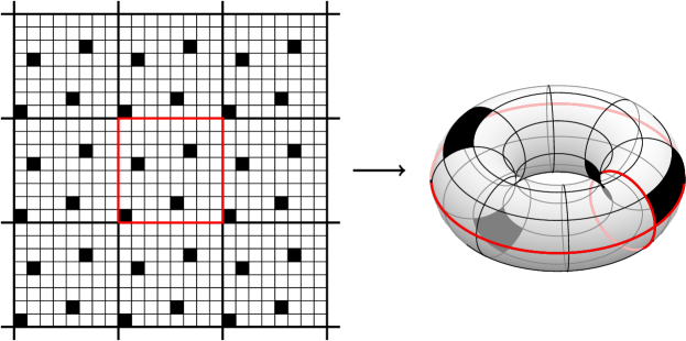
Figure 1: Example of a $n_{1}\times n_{2}=8\times 8$ grid tiling with $m=4$, and the corresponding toric interpretation of the $8\times 8$ grid.

We can then formulate this problem as QAP with matrices $A=(a_{ij}),B=(b_{ij})\in\mathbb{R}^{n\times n}$, indexed by grid points $i=(x_{i},y_{i})\in[n_{1}]\times[n_{2}]$, $j=(x_{j},y_{j})\in[n_{1}]\times[n_{2}]$, given by

$${\color[rgb]{0,0,0}a_{ij}}=\begin{cases}1,&\mbox{if }i,j\leq m\\ 0,&\mbox{otherwise}.\end{cases}, \qquad{\color[rgb]{0,0,0}b_{ij}}=f_{i,j}=f_{(x_{i},y_{i}),(x_{j},y_{j})}.$$ (3.3)

In the definition of $A$ we compared a grid point to an integer $m$. The ordering of the grid points does not matter for the optimal value or the symmetry reduction, so it is enough to assume that we have any fixed ordering of the indices, i.e. we may associate $[n]$ with $[n_{1}]\times[n_{2}]$ and will write $[n]=[n_{1}]\times[n_{2}]$ when convenient. We may also assume that the ordering is such that the nonzero elements of the matrix $A$ are given by the $m\times m$-block in the upper left corner, so that

$$\min_{\pi\in S_{n}}\sum_{i,j=1}^{n}a_{ij}b_{\pi(i)\pi(j)}=\min_{\pi\in S_{n}}\sum_{i,j\leq m}b_{\pi(i)\pi(j)}=\min_{\begin{subarray}{c}T\subseteq[n_{1}]\times[n_{2}]\\ |T|=m\end{subarray}}\sum_{a,b\in T}f_{a,b}$$ (3.4)

Note that the QAP has dimension $n=n_{1}\times n_{2}$, and its semidefinite relaxation has dimension $n^{2}$, which is already 4096 on an $8\times 8$ grid.

To reduce the number of cases one has to look at, we can show a that selecting the complement of an optimal solution leads to another optimal solution.

Proposition 3.1.

Consider a $[n]=[n_{1}]\times[n_{2}]$ grid, and a function $f\colon[n]\times[n]$ with $\sum_{j\in[n]}f(i,j)=\sum_{j\in[n]}f(j,i)=c$ for all $i\in[n]$ and a constant $c\in\mathbb{R}$ . Then, if $T\subseteq[n]$ minimizes

$$\min_{\begin{subarray}{c}T\subseteq[n_{1}]\times[n_{2}]\\ |T|=m\end{subarray}}\sum_{a,b\in T}f_{a,b},$$

then $S=[n]\setminus T$ minimizes

$$\min_{\begin{subarray}{c}S\subseteq[n_{1}]\times[n_{2}]\\ |S|=n-m\end{subarray}}\sum_{a,b\in S}f_{a,b}.$$

Proof.

We can rewrite the objective function as

$$\sum_{a,b\in T}f_{a,b} =\sum_{a,b\in[n]}f_{a,b}-\sum_{\begin{subarray}{c}a\notin T\\ b\in[n]\end{subarray}}f_{a,b}-\sum_{\begin{subarray}{c}a\in[n]\\ b\notin T\end{subarray}}f_{a,b}+\sum_{\begin{subarray}{c}a\notin T\\ b\notin t\end{subarray}}f_{a,b}$$

$$=cn-2c(n-m)+\sum_{a,b\in S}f_{a,b}.$$

Since the term $cn-2c(n-m)$ is independent of $T$ and $S$, minimizing $\sum_{a,b\in T}f_{a,b}$ is equivalent to minimizing $\sum_{a,b\in S}f_{a,b}$. ∎

3.1 Eigenvalue bound of Bouman, Draisma and Leeuwaarden

Problem (3.4) was considered before in [4], specifically for the case of the Lee-metric, and $m=\frac{n}{2}$ (which we can see as special case of our variant). They took a look at a different relaxation of the problem, which they call fractional total energy

$$\min\enspace x^{T}Bx$$ (3.5)

$$\mathrm{s.t.}\enspace x^{T}x=x^{T}e=m,$$

where $B=(b_{i,j})$ is the matrix of potential energies between grid points $i$ and $j$, as defined in 3.3. In the relaxation (3.5), the discrete variables $x_{i}$ correspond to particle positions, relaxed to continuous values. Thus if $x$ is the characteristic vector of a subset of $m$ particles, then it is exactly the potential energy of the set of particles. The optimal solution of the relaxation (3.5) may be expressed in terms of the eigenvalues of $B$ as follows.

Proposition 3.2 (Proposition 2.5. in [4]).

Let $\lambda_{\min}$ be the smallest eigenvalue of $B$, and $\lambda_{1}$ the eigenvalue of $B$ corresponding to $e$. Then the set of optimal solutions of the minimization problem (3.5) consists of all vectors of the form $\frac{m}{n}e+y$, where $y$ belongs to the eigenspace of $B$ with eigenvalue $\lambda_{\min}$, is perpendicular to $e$, and satisfies $y^{T}y=m-\frac{m^{2}}{n}$.

The optimal value, and thus a lower bound for the minimum potential energy of $m$ particles on a toric grid with $n$ nodes, is given by:

$$\lambda_{1}\frac{m^{2}}{n}+\lambda_{\min}\left(m-\frac{m^{2}}{n}\right).$$ (3.6)

We will from now on refer to the bound (3.6) as BDL-eigenvalue bound, named after the authors.

Remark 3.3.

The energy minimization problem on a toric grid is a special case of the so-called $m$-cluster problem, or minimum weight $m$-subgraph problem (see e.g. [19]). Indeed, the toric grid defines the graph in question, the edge weights are the energies between grid points, and the minimum weight $m$-subgraph corresponds to the $m$ grid points where the particles are placed in a minimum energy configuration. An SDP-bound with $n\times n$ matrix variables was proposed for the maximum weight $m$-subgraph problem in [19], which is of the form 3.7:

$$\inf\enspace \frac{1}{4}e^{T}Be+\frac{1}{2}e^{T}By+\frac{1}{4}\langle B,Y\rangle$$ (3.7)

$$\mathrm{s.t.}\enspace e^{T}y=2m-n,$$

$$\sum_{i}Y_{ij}=(2m-n)y_{j}\quad\text{for }j=1,\ldots,n,$$

$$Y_{ii}=1\quad\text{for }i=1,\ldots,n,$$

$$\begin{pmatrix}1&y^{T}\\ y&Y\end{pmatrix}\succcurlyeq 0.$$

It is straightforward to check that this bound is at most as good as (3.5) for our problem. Indeed, since the weighted graph given by $B$ is vertex transitive, we obtain a feasible solution $(Y,y)$ for (3.7) (with the same objective value) from a feasible solution $x$ for (3.5) by setting

$$y=\mathrm{sym}(2x-e)=\left(\frac{2m}{n}-1\right)e\text{ and }Y=\mathrm{R}((2x-e)(2x-e)^{T}),$$

where $\mathrm{sym}$ averages a vector over the orbits of the automorphism group of the graph given by $B$, and $\mathrm{R}$ is the Reynolds operator of the same group (i.e. it averages matrix entries over the $2$-orbits of the group). Thus this bound is not strong enough to improve the BDL-eigenvalue bound (3.6).

3.2 Bound comparison

We now want to compare the BDL-eigenvalue bound with the QAP relaxations described last section, as well as the different QAP relaxations for this specific case.

Proposition 3.4.

The BDL-eigenvalue bound of [4], see (3.6), coincides with the projected eigenvalue bound (see Proposition 2.1) for the QAP problem (3.4).

Proof.

The matrix $D$ in Proposition 2.1 is now given by

$$D=\frac{2}{n}Aee^{T}B=\lambda_{1}\frac{2}{n}(\underbrace{m,\ldots,m}_{m\text{ times}},0,\ldots,0)^{T}e^{T},$$

and thus has entries $\lambda_{1}\frac{2m}{n}$ in the first $m$ rows, and zeros otherwise. As such, the permutation $\varphi$ does not influence the result, and

$$\min_{\varphi}\sum_{i=1}^{n}d_{i\varphi(i)}=\lambda_{1}\frac{2m^{2}}{n}.$$ (3.8)

We know that $e$ is an eigenvector of $B$, hence we have

$$\frac{(e^{T}Ae)(e^{T}Be)}{n^{2}}=\frac{m^{2}\lambda_{1}n}{n^{2}}=\lambda_{1}\frac{m^{2}}{n}.$$

The matrix $A$ has rank one, so $\tilde{A}$ has rank one as well. Since $e$ is an eigenvector of $B$, $\tilde{B}$ has the same eigenvalues as $B$, except for $\lambda_{1}$, thus we get

$$\langle\lambda_{\tilde{A}},\mu_{\tilde{B}}\rangle^{-}=\lambda_{\max}(\tilde{A})\lambda_{\min}(\tilde{B})=\mathrm{tr}(\tilde{A})\lambda_{\min}.$$

The eigenvalue of $\tilde{A}$ is exactly

$$\mathrm{tr}(\tilde{A}) =\mathrm{tr}(V^{T}AV),$$

$$=\mathrm{tr}(A)-\frac{1}{n}\mathrm{tr}(AJ),$$

$$=m-\frac{m^{2}}{n}.$$

Combining these, we see that the projection bound is the same as the eigenvalue bound:

$$PB(A,B) =\langle\lambda_{\tilde{A}},\mu_{\tilde{B}}\rangle^{-}+\min_{\varphi}\sum_{i=1}^{n}d_{i\varphi(i)}-\frac{(e^{T}Ae)(e^{T}Be)}{n^{2}}$$

$$=\lambda_{1}\frac{m^{2}}{n}+\lambda_{\min}\left(m-\frac{m^{2}}{n}\right).$$

∎

Thus the BDL-eigenvalue bound (3.6) is the same as the weakest of the QAP bounds we considered, namely the bound $PB(A,B)$. Furthermore, even the convex quadratic bound cannot give us better bounds here, as we show now.

Proposition 3.5.

If $A$ and $B$ are of the form

$${\color[rgb]{0,0,0}a_{ij}}=\begin{cases}1,&\mbox{if }i,j\leq m\\ 0,&\mbox{otherwise}.\end{cases}, \quad{\color[rgb]{0,0,0}b_{i,j}}=f_{i,j}=f_{(x_{i},y_{i}),(x_{j},y_{j})},$$

as defined for the energy minimization problem, then we have that

$$PB(A,B)=QPB(A,B),$$

where

$$PB(A,B)=\langle\lambda_{\tilde{A}},\mu_{\tilde{B}}\rangle^{-}+\min_{\varphi}\sum_{i=1}^{n}d_{i\varphi(i)}-\frac{(e^{T}Ae)(e^{T}Be)}{n^{2}}$$

$$QPB(A,B)=\min_{\begin{subarray}{c}X\geq 0\text{ doubly stochastic}\\ X=\frac{1}{n}ee^{T}+VYV^{T}\\ y=\mathrm{vec}(Y)\end{subarray}}y^{T}\hat{Q}y+\langle\lambda_{\tilde{A}},\mu_{\tilde{B}}\rangle^{-}+\frac{2}{n}\mathrm{tr}\left(BJAX\right)-\frac{(e^{T}Ae)(e^{T}Be)}{n^{2}},$$

where $D=(d_{ij})=\frac{2}{n}AJB$ and $\hat{Q}$ is positive semidefinite, as defined before (see (2.1), (2.2)).

Proof.

If we eliminate the terms which appear in both programs, we see that we want to show

$$\min_{\varphi}\sum_{i=1}^{n}d_{i\varphi(i)}=\min_{\begin{subarray}{c}X\geq 0\text{ doubly stochastic}\\ X=\frac{1}{n}ee^{T}+VYV^{T}\\ y=\mathrm{vec}(Y)\end{subarray}}y^{T}\hat{Q}y+\frac{2}{n}\mathrm{tr}\left(BJAX\right).$$

By definition of $D$ the two linear terms are equal, except that on the left we minimize over permutations, and on the right over doubly stochastic matrices. Because the terms are linear, and doubly stochastic matrices are convex combinations of permutations, the minima of the two linear terms are equal. Since $\hat{Q}$ is positive semidefinite, we thus want to find a doubly stochastic $X=\frac{1}{n}J+VYV^{T}$ with $y^{T}\hat{Q}y=0$, which minimizes the linear term. Earlier in (3.8) we have seen that

$$\sum_{i=1}^{n}d_{i\varphi(i)}=\lambda_{1}\frac{2m^{2}}{n}\quad\forall\varphi,$$

and is thus the linear term is constant. Hence the term is also minimized for the average $X=\frac{1}{n}J$ of all permutations. For this $X$ we have $Y=\frac{1}{n}V^{T}JV=0$, and consequently $y^{T}\hat{Q}y=0$. Thus there is a feasible $X$ of $QPB(A,B)$ with objective value $PB(A,B)$, and the Proposition follows since $QPB(A,B)\geq PB(A,B)$. ∎

Thus it makes sense to consider the SDP-bound $SDPQAP(A,B)$ for the energy minimization QAP problem (3.3), if one wants to find stronger bounds than the BDL-bound used in [4].

4 Reducing the relaxation of the energy minimization problem

In this section we exploit the symmetry of the SDP-bound SDPQAP in the case of the energy minimization problem. Recall from Section 3, and with reference to Figure 1, that this is a quadratic assignment problem given by $A$ and $B$, where $B=(b_{ij})$ is indexed by toric grid points, and $b_{ij}$ $(i\neq j)$ equals the inverse of the Lee distance (shortest path on the grid) between grid points $i$ and $j$, and $b_{ii}=0$ for all $i$. The matrix $A$ is zero except for a square block of all-ones in the upper left corner, of size equal to the number of particles on the toric grid. There are many approaches to exploit the symmetry of a conic optimization problem. Earlier work on group-theoretical symmetry reductions of SDP bounds for QAP was done in [9, 10]. We chose to apply the Jordan Reduction method of Parrilo and Permenter [20] to our problem, which we will quickly summarize.

4.1 The Jordan Reduction

Parrilo and Permenter [20] introduced a set of three conditions a subspace has to fulfill, such that it is be possible to use it for symmetry reduction. Here we revisit some of their results.

Definition 4.1.

A projection is a linear transformation $P\colon\mathcal{V}\to\mathcal{V}$ defined on a vector space $\mathcal{V}$ which is idempotent, i.e. $P^{2}=P$. If $\mathcal{V}$ is equipped with an inner product, the projection is called orthogonal, if it is self-adjoint with respect to this inner product. We denote the orthogonal projection onto a subspace $\mathcal{L}\subset\mathcal{V}$ by $P_{\mathcal{L}}$.

We assume that the problem to be reduced is in the form

$$\left.\begin{array}[]{llrl}\inf&\langle C,X\rangle\\ \mathrm{s.t.}&X\in X_{0}+\mathcal{L}\\ &X\in S^{n}_{+},\end{array}\right\}$$ (4.1)

where $X_{0}\in\mathbb{R}^{n\times n}$, and $\mathcal{L}$ is a linear subspace of $\mathbb{R}^{n\times n}$.

Theorem 4.2 (Theorem 5.2.4 and Proposition 1.4.1 in [21]).

Consider the conic optimization problem (4.1) and let $S\subseteq\mathbb{R}^{n\times n}$ be a subspace of $\mathbb{R}^{n\times n}$. Define $C_{\mathcal{L}}=P_{\mathcal{L}}(C)$ and $X_{0,\mathcal{L}^{\perp}}=P_{\mathcal{L}^{\perp}}(X_{0})$. If $S$ fulfills

• $C_{\mathcal{L}},X_{0,\mathcal{L}^{\perp}}\in S$,

• $P_{\mathcal{L}}(S)\subseteq S$,

• $S\supseteq\{X^{2}\enspace\colon\enspace X\in S\}$,

then restricting the feasible set of conic program (4.1) to $S$ results in another — potentially significantly smaller — program, with the same optimal value:

$$\inf\enspace \langle P_{S}(C),X\rangle$$

$$\mathrm{s.t.}\enspace X\in P_{S}(X_{0})+\mathcal{L}\cap S,$$

$$X\in S^{n}_{+}\cap S.$$

We call such an $S$ admissible for the problem (4.1).

We will use the concept of a Jordan algebra: for our purposes this will be a subspace of symmetric matrices that is closed under the product $X\circ Y=\frac{1}{2}(XY+YX)$. It follows from condition (c) in the theorem that every admissible subspace is a Jordan algebra. Indeed, a subspace of symmetric matrices is a Jordan algebra if and only if it is closed under taking squares, due to the identity $X\circ Y=\frac{1}{2}\left((X+Y)^{2}-X^{2}-Y^{2}\right).$ We will denote the full Jordan algebra of symmetric $n\times n$ matrices by $\mathbb{S}^{n}$.

Note that, for the SDP-bound SDPQAP, one would actually use the cone of entry-wise nonnegative matrices (i.e. doubly nonnegative matrices), as opposed to $S^{n}_{+}$. To deal with the nonnegativity, we will in fact work with admissible subspaces that have 0-1 bases and where the basis matrices have disjoint support (so-called partition subspaces).

4.2 Symmetric circulant matrices

First, we need some well-known properties of (symmetric) circulant matrices, which will appear later in the construction of the admissible subspaces of the relaxation of the energy minimization problem.

Definition 4.3.

An $n\times n$ matrix $C$ is called circulant, if each row is rotated one element to the right relative to the row above, i.e. $C_{ij}=c_{j-i\mod n}$ for all $i,j$ and fitting $c_{k}$, $k=0,\ldots,n-1$.

Proposition 4.4.

A symmetric circulant $n\times n$ matrix $C$ has at most $\lfloor\frac{n}{2}\rfloor+1=\lceil\frac{n+1}{2}\rceil$ unique entries, and $c_{k}=c_{n-k}$.

Proof.

Let $j\geq i$ and $k=j-i$. By definition we have $c_{k}=C_{ij}=C_{ji}=c_{n-(j-i)}=c_{n-k}$. Hence $C$ is given by $c_{0},\ldots,c_{\lfloor\frac{n}{2}\rfloor}$. ∎

This allows us to construct symmetric circulant matrices from a given $c\in\mathbb{R}^{\lceil\frac{n+1}{2}\rceil}$. We call this function $C=\mathrm{circ}_{n}(c_{0},\ldots,c_{\lfloor\frac{n}{2}\rfloor})$.

Proposition 4.5 (E.g. Theorem 7 in [13]).

The product of two circulant matrices is a circulant matrix, and the product commutes. The product of symmetric circulant matrices is symmetric.

We call the Jordan algebra (with product $X\circ Y=\frac{1}{2}(XY+YX)=XY$) of symmetric circulant $n\times n$ matrices $\mathfrak{C}^{n}$. We define a $0/1$-basis for $\mathfrak{C}^{n}$ by

$$\left\{C^{n}_{i}=\mathrm{circ}_{n}(d_{i})\enspace\colon\enspace i=0,\ldots,\lfloor\frac{n}{2}\rfloor\right\},$$ (4.2)

where for $i\notin\{0,\frac{n}{2}\}$ we set $d_{i}=e_{i}\in\mathbb{R}^{\lfloor\frac{n}{2}\rfloor+1}$, the vector with a one in position $i$, and zero otherwise. For $i=0$ and $i=\frac{n}{2}$, if $n$ is even, we set $d_{i}=2e_{i}$.

4.3 Admissible subspaces

To reduce the program $SDPQAP(A,B)$ in (2.3) for the energy minimization problem (3.3), one should find an admissible subspace $S$ for every such problem. In this case $\mathcal{L}$ is the subspace given by the $Y\in{\mathbb{S}}^{n^{2}}$ with

$$\langle I_{n}\otimes E_{jj},Y\rangle =0\text{ for }j\in[n],$$

$$\langle E_{jj}\otimes I_{n},Y\rangle =0\text{ for }j\in[n],$$

$$\langle T,Y\rangle =0,$$

$$\langle J_{n^{2}},Y\rangle =0,$$

where $T=I_{n}\otimes(J_{n}-I_{n})+(J_{n}-I_{n})\otimes I_{n}$, and $X_{0}$ is any symmetric matrix satisfying the linear constraints of the SDP (2.3), e.g. $X_{0}=\mathrm{vec}(I_{n})\mathrm{vec}(I_{n})^{T}$.

Note here that we are missing the constraint that $X$ is entry-wise nonnegative. But it is easy to check that if we restrict $S$ to be a partition subspace (i.e. a subspace with an orthogonal $0/1$-basis), then $P_{S}(X)$ is doubly-nonnegative if $X$ is.

Recall that, for $n=n_{1}n_{2}$, the matrix $B\in\mathbb{R}^{n\times n}$ is defined by $B_{(x_{1},y_{1}),(x_{2},y_{2})}=1/d_{\mathrm{Lee}}((x_{1},y_{1}),(x_{2},y_{2}))$, where $d_{\mathrm{Lee}}$ is the Lee-distance (length of shortest path on the toric grid). The ordering of the indices $[n_{1}]\times[n_{2}]=[n]$ we left implicit in earlier sections of this paper, but now we fix it to $(x,y)\mapsto n_{2}(x-1)+y$. $A\in\mathbb{R}^{n\times n}$ is the matrix with an $m\times m$ all-one block in the top left corner, and otherwise zero.

In this section we will make use of Tensor products of algebras. As a reminder, if $A_{1},\ldots,A_{d_{1}}\in\mathbb{R}^{n_{1}\times n_{1}}$ is a basis of a matrix algebra $\mathcal{A}$, and $B_{1},\ldots,B_{d_{2}}\in\mathbb{R}^{n_{2}\times n_{2}}$ a basis of a matrix algebra $\mathcal{B}$, then $\mathcal{A}\otimes\mathcal{B}$ is the $n_{1}n_{2}\times n_{1}n_{2}$ matrix algebra with basis $A_{i}\otimes B_{j}$, for $i\in[d_{1}],j\in[d_{2}]$.

We restrict ourselves to a partition subspace, which means that the exact values of the entries of the matrix do not matter to us, only the pattern of unique elements. For the first of the three properties, we take a look at the structure of $\mathbf{C}\coloneqq B\otimes A$.

Lemma 4.6.

$B\in\mathfrak{C}^{n_{1}}\otimes\mathfrak{C}^{n_{2}}$, i.e. $B$ is a block matrix, with $n_{1}$ rows and columns of blocks, which are arranged in a symmetric circulant pattern, and each of these blocks is an $n_{2}\times n_{2}$ symmetric circulant matrix.

Proof.

The Lee-distance between $(x_{1},y_{1})$ and $(x_{2},y_{2})$ depends only on $x_{2}-x_{1}\mod n_{1}$ and $y_{2}-y_{1}\mod n_{2}$, and the order of the arguments do not matter. This means that both the submatrices for fixed $x$ and for fixed $y$ coordinates are symmetric circulant matrices:

$$\left(B_{(i,y_{1}),(j,y_{2})}\right)_{1\leq i,j,\leq n_{1}}\in\mathfrak{C}^{n_{1}}, \left(B_{(x_{1},i),(x_{2},j)}\right)_{1\leq i,j,\leq n_{2}}\in\mathfrak{C}^{n_{2}}.$$

The chosen ordering of the indices $(x,y)\mapsto n_{2}(x-1)+y$ thus results in $B\in\mathfrak{C}^{n_{1}}\otimes\mathfrak{C}^{n_{2}}$. ∎

In the case $n_{1}=n_{2}$ we can restrict the algebra further.

Lemma 4.7.

If $n_{1}=n_{2}$, then

$$B\in\mathfrak{C}^{n_{1},n_{1}}\coloneqq\left\{X\in\mathfrak{C}^{n_{1}}\otimes\mathfrak{C}^{n_{1}}\enspace\colon\enspace X_{(x_{1},y_{1}),(x_{2},y_{2})}=X_{(y_{1},x_{1}),(y_{2},x_{2})}\right\},$$ (4.3)

and $\mathfrak{C}^{n_{1},n_{1}}$ is a Jordan sub-algebra of $\mathfrak{C}^{n_{1}}\otimes\mathfrak{C}^{n_{1}}$.

Proof.

$B$ is has this symmetry by definition of the Lee-distance. $\mathfrak{C}^{n_{1},n_{1}}$ is a sub-algebra, because it is the restriction of an algebra to the commutant of $\{P,I\}$, where $P$ is the $n\times n$ permutation matrix switching the indices corresponding to each $(x,y)$ with the one corresponding to $(y,x)$. ∎

The other relevant Jordan algebra for our problem is described in the following proposition.

Proposition 4.8.

The subspace of $n\times n$ matrices with pattern

form a Jordan algebra, say $\mathcal{J}^{n,m}$. We call the $0/1$-basis corresponding to this pattern $J_{A},J_{B},J_{C},J_{D},J_{E}$.

Proof.

A straightforward calculation shows that squaring such a matrix results in another matrix of the same pattern with parameters

$$a^{\prime} =a^{2}+(m-1)b^{2}+(n-m)c^{2},$$

$$b^{\prime} =2ab+(m-2)b^{2}+(n-m)c^{2},$$

$$c^{\prime} =(a+(m-1)b)c+(d+(n-m-1)e)c,$$

$$d^{\prime} =d^{2}+(n-m-1)e^{2}+mc^{2},$$

$$e^{\prime} =2de+(n-m-2)e^{2}+mc^{2}.$$

∎

We now want to show that the space $S\coloneqq\mathfrak{C}^{n_{1}}\otimes\mathfrak{C}^{n_{2}}\otimes\mathcal{J}^{n,m}$, respectively $S=\mathfrak{C}^{n_{1},n_{1}}\otimes\mathcal{J}^{n,m}$ if $n_{1}=n_{2}$, is admissible. We do this by verifying the three conditions listed in Theorem 4.2.

Theorem 4.9.

The subspace $S\coloneqq\mathfrak{C}^{n_{1}}\otimes\mathfrak{C}^{n_{2}}\otimes\mathcal{J}^{n,m}$, respectively $S=\mathfrak{C}^{n_{1},n_{1}}\otimes\mathcal{J}^{n,m}$ if $n_{1}=n_{2}$ is admissible for (2.3), where $B$ and $A$ are the matrices corresponding to the problem of minimizing the energy of $m$ particles on an $n_{1}\times n_{2}$ grid.

For $2<m<n-2$ the dimension of $S$ is $5\lceil\frac{n_{1}+1}{2}\rceil\lceil\frac{n_{2}+1}{2}\rceil$ in the case $n_{1}\neq n_{2}$, and $\frac{5}{2}\lceil\frac{n_{1}+1}{2}\rceil\left(\lceil\frac{n_{2}+1}{2}\rceil+1\right)$ in the case $n_{1}=n_{2}$.

Proof.

We first show that $P_{\mathcal{L}}(S)\subseteq S$. To this end, note that both $T=I_{n}\otimes(J_{n}-I_{n})+(J_{n}-I_{n})\otimes I_{n}$ and $J_{n^{2}}$ are elements of $S$, since $J_{n}=J_{n_{1}}\otimes J_{n_{2}}$ and $I_{n}=I_{n_{1}}\otimes I_{n_{2}}$ are both in $\mathfrak{C}^{n_{1}}\otimes\mathfrak{C}^{n_{2}}$ (and in $\mathfrak{C}^{n_{1},n_{1}}$ if $n_{1}=n_{2}$), as well as in $\mathcal{J}^{n,m}$ because $I_{n}=J_{A}+J_{D}$ and $J_{n}=I_{n}+J_{B}+J_{C}+J_{E}$. Thus $T$ and $J_{n^{2}}$ can be written as linear combination of Kronecker products of elements of $\mathfrak{C}^{n_{1}}$, $\mathfrak{C}^{n_{2}}$ and $\mathcal{J}^{n,m}$, and are as such elements of $S$.

The other two constraints are given by matrices $I_{n}\otimes E_{jj}$ and $E_{jj}\otimes I_{n}$, which only overlap with the two basis elements $C^{n_{1}}_{0}\otimes C^{n_{2}}_{0}\otimes J_{A}$ and $C^{n_{1}}_{0}\otimes C^{n_{2}}_{0}\otimes J_{D}$. Since $C^{n_{1}}_{0}\otimes C^{n_{2}}_{0}\otimes J_{A}=\sum_{j=1}^{m}I_{n}\otimes E_{jj}$ and $C^{n_{1}}_{0}\otimes C^{n_{2}}_{0}\otimes J_{D}=\sum_{j=m+1}^{n}I_{n}\otimes E_{jj}$, both of these matrices are projected to zero.

Thus all basis elements of $S$ are sent to elements of $S$, and $P_{\mathcal{L}}(S)\subseteq S$.

Next, we show $\mathbf{C}_{\mathcal{L}}\in S$. By Lemma 4.6, Lemma 4.7 and the definition of $A$, we know that $C=B\otimes A\in S$. Since $P_{\mathcal{L}}(S)\subseteq S$, that $\mathbf{C}_{\mathcal{L}}\in S$ as well.

Next, we show that $X_{0,\mathcal{L}^{\perp}}\in S$. To project $X_{0}=\mathrm{vec}(I_{n})\mathrm{vec}(I_{n})^{T}$ onto $\mathcal{L}^{\perp}$, the span of the constraint matrices, we first notice only two of them have nonzero entries outside of the diagonal, the all one matrix $J_{n^{2}}$, and the matrix $I_{n}\otimes(J_{n}-I_{n})+(J_{n}-I_{n})\otimes I_{n}$, which we will call $T$ from now on. The matrices $I_{n}\otimes E_{jj}$ for $j=1,\ldots,n$ sum to the identity matrix $I_{n^{2}}$, which means that we can easily find an orthogonal basis of the off diagonal part of $\mathcal{L}^{\perp}$:

$$B_{1} =T,$$

$$B_{2} =J_{n^{2}}-I_{n^{2}}-T.$$

Since $\langle T,X_{0}\rangle=0$ and $\langle J_{n^{2}},X_{0}\rangle=n^{2}$ we get

$$\langle B_{2},X_{0}\rangle=\langle J_{n^{2}},X_{0}\rangle-\langle I_{n^{2}},X_{0}\rangle=n^{2}-n.$$

Hence the off-diagonal part of $X_{0,\mathcal{L}^{\perp}}$ is the matrix

$$\frac{\langle B_{2},X_{0}\rangle}{\langle B_{2},B_{2}\rangle}B_{2}=\frac{n^{2}-n}{n^{4}-n^{2}-2n(n^{2}-n)}B_{2}=\frac{1}{n^{2}-n}B_{2}.$$

The diagonal part of $X_{0,\mathcal{L}^{\perp}}$ is the matrix $\frac{1}{n}I_{n^{2}}$, since

$$\langle E_{jj}\otimes I_{n},\frac{1}{n}I_{n^{2}}-X_{0}\rangle =\langle E_{jj}\otimes I_{n},\frac{1}{n}I_{n^{2}}\rangle-\langle E_{jj}\otimes I_{n},X_{0}\rangle=1-1=0,$$

and analogously $\langle I_{n}\otimes E_{jj},\frac{1}{n}I_{n^{2}}-X_{0}\rangle=0$. Combining the two parts we see

$$X_{0,\mathcal{L}^{\perp}}=\frac{1}{n^{2}-n}B_{2}+\frac{1}{n}I_{n^{2}}.$$

Since $J_{n^{2}}$, $I_{n^{2}}$ and $T$ are elements of $S$, we get that $X_{0,\mathcal{L}^{\perp}}\in S$.

Finally, we note that $S$ is a Jordan algebra. This completes the proof that $S$ is admissible. The dimension of $S$ follows from $\mathfrak{C}^{n}$ having dimension $\lceil\frac{n+1}{2}\rceil$ and $\mathcal{J}^{n,m}$ having dimension $5$. In the case $n_{1}=n_{2}$ the dimension is lower, since we can combine the basis elements $C^{n_{1}}_{i}\otimes C^{n_{1}}_{j}$ and $C^{n_{1}}_{j}\otimes C^{n_{1}}_{i}$ for each pair $i\neq j$. ∎

Thus we have found an admissible subspace $S$ for (2.3), where $A$ and $B$ are the matrices corresponding to the problem of minimizing the energy of $m$ particles on an $n_{1}\times n_{2}$ toric grid. Its dimension is of order $\mathcal{O}(n_{1}n_{2})$, which is significantly less than the original number of variables $\frac{n_{1}^{4}n_{2}^{4}+n_{1}^{2}n_{2}^{2}}{2}=\mathcal{O}(n_{1}^{4}n_{2}^{4})$. The number of variables can be reduced further by fixing the variables corresponding to nonzero entries of $I_{n}\otimes(J_{n}-I_{n})+(J_{n}-I_{n})\otimes I_{n}$ to zero. Thus if $\{B_{1},\ldots,B_{k}\}$ is a $0/1$-basis of an admissible subspace, then it is enough to optimize over variables in the subspace $S_{0}$ with basis

$$\left\{B_{i}\enspace\colon\enspace\langle B_{i},I_{n}\otimes(J_{n}-I_{n})+(J_{n}-I_{n})\otimes I_{n}\rangle=0\right\}.$$

This results in $3\lceil\frac{n_{1}+1}{2}\rceil\lceil\frac{n_{2}+1}{2}\rceil-1$ variables in the case $n_{1}\neq n_{2}$, and $1.5\lceil\frac{n_{1}+1}{2}\rceil\left(\lceil\frac{n_{2}+1}{2}\rceil+1\right)-1$ variables in the case $n_{1}=n_{2}$. A few examples can be seen in Table 1. Note that the resulting subspace is generally not a Jordan algebra anymore.

Table 1: Number of variables before and after symmetry reduction.

$(n_{1},n_{2})$	$\mathrm{dim}({\mathbb{S}}^{n_{1}^{2}n_{2}^{2}})$		$\mathrm{dim}(S)$	$\mathrm{dim}(S_{0})$
$(4,4)$	32896		30	17
$(5,5)$	195625		30	17
$(6,6)$	840456		50	29
$(8,8)$	8390656		75	44
$(10,10)$	50005000		105	62
$(12,12)$	215001216		140	83
$(24,24)$	55037822976		455	272
$(100,100)$	$\approx 5\cdot 10^{15}$		6630	3977
$(1000,1000)$	$\approx 5\cdot 10^{23}$		628755	377252
$(6,5)$	405450		60	35
$(10,5)$	3126250		90	53
$(24,12)$	3439895040		455	272

4.4 Block diagonalization

We now want to block diagonalize the admissible subspace $S\coloneqq\mathfrak{C}^{n_{1}}\otimes\mathfrak{C}^{n_{2}}\otimes\mathcal{J}^{n,m}$, respectively $S=\mathfrak{C}^{n_{1},n_{1}}\otimes\mathcal{J}^{n,m}$ if $n_{1}=n_{2}$. We do this by making use of the fact that $S$ is a tensor product of algebras, which allows us to block diagonalize each part on its own.

Lemma 4.10 (See, for example, [13], [8]).

The $0/1$-basis $\{C_{i}^{n}\enspace\colon\enspace i=0,\ldots,\lfloor\frac{n}{2}\rfloor\}$ of $\mathfrak{C}^{n}$ has a common set of eigenvectors, given by the columns of the discrete Fourier transform matrix:

$$Q^{n}_{ij}\coloneqq\frac{1}{\sqrt{n}}e^{-2\pi\sqrt{-1}ij/n},\qquad i,j=0,\ldots,n-1.$$

The eigenvalues are

$$\lambda_{m}(C_{k}^{n})=2\cos(2\pi mk/n),\qquad m=0,\ldots,n-1,k=0,\ldots,\lfloor\frac{n}{2}\rfloor,$$

and note that

$$\lambda_{m}(C_{k}^{n})=\lambda_{n-m}(C_{k}^{n}),\qquad m=1,\ldots,\lfloor\frac{n}{2}\rfloor,k=0,\ldots,\lfloor\frac{n}{2}\rfloor.$$

Thus we can block diagonalize $\mathfrak{C}^{n}$ by sending $C_{k}^{n}$ to the vector

$$\hat{\lambda}(C_{k}^{n})\coloneqq(\lambda_{0}(C_{k}^{n}),\ldots,\lambda_{\lfloor\frac{n}{2}\rfloor}(C_{k}^{n})).$$

To block diagonalize $\mathcal{J}^{n,m}$, one may use the Jordan isomorphism $\phi:\mathcal{J}^{n,m}\rightarrow\mathbb{R}\oplus\mathbb{R}\oplus\mathbb{S}^{2}$ given by

$$\phi(J_{A})=\left(\begin{smallmatrix}n-m\\ &0\\ &&1&0\\ &&0&0\\ \end{smallmatrix}\right),\;\phi(J_{B})=\left(\begin{smallmatrix}-1\\ &0\\ &&m-1&0\\ &&0&0\\ \end{smallmatrix}\right),\;\phi(J_{C})=\sqrt{m(n-m)}\left(\begin{smallmatrix}0\\ &0\\ &&0&1\\ &&1&0\\ \end{smallmatrix}\right),$$

$$\phi(J_{D})=\left(\begin{smallmatrix}0\\ &1\\ &&0&0\\ &&0&1\\ \end{smallmatrix}\right),\;\phi(J_{E})=\left(\begin{smallmatrix}0\\ &-1\\ &&0&0\\ &&0&n-m-1\\ \end{smallmatrix}\right).$$

This isomorphism was used implicitly in [7], but may also be verified directly by confirming that $\phi(X^{2})=[\phi(X)]^{2}$ for all $X\in\mathcal{J}^{n,m}$.

We can now combine these block diagonalizations by noticing that it is enough to block diagonalize each of the algebras separately; see, for example, Section 7.2. in [9]. We obtain the final reduction shown in the next theorem. The proof is omitted since it is straightforward: One just has to calculate the inner products between the basis elements of the algebra and the data matrices, and eliminate variables fixed to zero by $\langle B_{i},I_{n}\otimes(J_{n}-I_{n})+(J_{n}-I_{n})\otimes I_{n}\rangle=0$. We then further scaled some variables and matrices to simplify terms further.

In the following we use the constants

$$d^{kl}_{ij}\coloneqq\cos\left(\frac{2\pi ki}{n_{1}}\right)\cos\left(\frac{2\pi lj}{n_{2}}\right),$$

which arise from the diagonalization of the circulant matrices.

Theorem 4.11.

The bound from (2.3), where the matrices $A,B$ correspond to the energy minimization problem with parameters $n_{1}$, $n_{2}$, $n=n_{1}n_{2}$ and $m$, equals the optimal value of the following semidefinite program:

$$\inf\enspace n\sum_{i+j>0}\frac{y^{b\to b}_{ij}}{i+j}$$ (4.4)

$$\mathrm{s.t.}\enspace \sum_{i+j>0}\left(y^{b\to b}_{ij}+y^{w\to w}_{ij}+y^{b\leftrightarrow w}_{ij}\right)=n-1,$$ (4.5)

$$\text{for all }0\leq k\leq\left\lfloor\frac{n_{1}}{2}\right\rfloor,0\leq l\leq\left\lfloor\frac{n_{2}}{2}\right\rfloor\colon$$ (4.6)

$$\quad\begin{pmatrix}\frac{m}{n}&0\\ 0&\frac{n-m}{n}\end{pmatrix}+\sum_{i+j>0}d^{kl}_{ij}\begin{pmatrix}y^{b\to b}_{ij}&\frac{1}{2}y^{b\leftrightarrow w}_{ij}\\ \frac{1}{2}y^{b\leftrightarrow w}_{ij}&y^{w\to w}_{ij}\end{pmatrix}\succcurlyeq 0,$$ (4.7)

$$\quad\frac{m(m-1)}{n}-\sum_{i+j>0}d^{kl}_{ij}y^{b\to b}_{ij}\geq 0,$$ (4.8)

$$\quad\frac{(n-m)(n-m-1)}{n}-\sum_{i+j>0}d^{kl}_{ij}y^{w\to w}_{ij}\geq 0,$$ (4.9)

$$y_{ij}^{b\to b},y_{ij}^{w\to w},y_{ij}^{b\leftrightarrow w}\geq 0\;\forall(i,j)\enspace|\enspace i+j>0,\enspace i\in\left\{0,\ldots,\left\lfloor\frac{n_{1}}{2}\right\rfloor\right\},\enspace j\in\left\{0,\ldots,\left\lfloor\frac{n_{2}}{2}\right\rfloor\right\}.$$ (4.10)

We can interpret the variables as averaged occurrences of pairs of black points ($b\to b$), pairs of white points ($w\to w$), and pairs of a white and a black point ($b\to w$), at distance $(i,j)$. I.e. if we have a given configuration, we can count how many pairs of points at distance $(i,j)$ are both black, and then set $y^{b\to b}_{ij}$ to this value divided by the total number of pairs, to construct a feasible solution. Variables corresponding to distances bigger than $\left\lfloor\frac{n_{1}}{2}\right\rfloor$ respectively $\left\lfloor\frac{n_{2}}{2}\right\rfloor$ are looped around and added onto smaller distance variables, i.e. we may have variable values bigger than one.

The semidefinite program in Theorem 4.11 has block sizes of order at most $2\times 2$, and is therefore a second-order cone program, which can be solved very efficiently; see e.g. [17]. Thus we were able to solve the SDP relaxation for toric grids of sizes up to $100\times 100$. Subsequently we were also able to prove optimality of certain configurations of particles on toric grids, as detailed in the next section.

5 Numerical results

Here we compare the eigenvalue-bound with the SDP-bound for the energy minimization problems. The upper bounds were found using simulated annealing (see Algorithm 1).

$iter\leftarrow$ number of iterations to perform

$P\leftarrow$ random configuration of $m$ particles

$val\leftarrow$ energy of P $=E(P)$

$T\leftarrow 1$

$a\leftarrow\sqrt[iter]{\frac{1}{iter}}$

for $it\leftarrow 1$ to iterations do

       $T\leftarrow aT$

       $P^{\prime}\leftarrow P$

       Move a random particle of $P^{\prime}$ to a neighbouring position

      

      if $E(P^{\prime})<val$ or $\exp(-(E(P^{\prime})-val)/T)\geq\mathrm{rand}(0,1)$ then

             $val\leftarrow E(P^{\prime})$

             $P\leftarrow P^{\prime}$

      

return $val$

Algorithm 1 Simulated annealing algorithm

Calculating the SDP-bound directly is prohibitively slow, which is why we symmetry reduced the problems first, as described in Section 4. After this reduction we can calculate these bounds very efficiently, solving a case of the problem on a $10\times 10$-grid in 0.2s, 1.3s on a $50\times 50$-grid, and in about 40s on $100\times 100$-grid, using Mosek on a 4-core 3.4GHz Processor. In [4] Bouman, Draisma and van Leeuwaarden prove optimality for the checkerboard arrangement in the cases that $n_{1}=n_{2}$ are even, and $m=\frac{n_{1}n_{2}}{2}$. This can be seen for the grid sizes we checked as well, but we do get some more proofs of optimality.

If one of the bounds is sharp, then we get a proof of optimality for these parameters. Furthermore, we can even prove optimality in some cases even if the bound is not completely sharp, as explained in the following result.

Proposition 5.1.

Let $V=\{v_{1},\ldots,v_{k}\}$ be the set of unique entries of the matrix of potentials $B$. The one-dimensional shortest-vector-problem for these values is

$$r=\min\enspace |s-t|$$

$$\mathrm{s.t.}\enspace s,t\in\left\{x=2\sum_{i=1}^{k}\alpha_{i}v_{i}\enspace|\enspace\alpha_{i}\in\mathbb{Z}\right\}$$

$$s\neq t.$$

If a feasible solution of the QAP has objective value that differs by less than $r$ from the SDP lower bound, then this feasible solution is optimal.

Proof.

Both the matrix $A$ and the optimization variable $X\in\Pi_{n}$ of this QAP are symmetric $0/1$-matrices, and $B$ is symmetric as well, with zeros on the main diagonal, which means that the objective value is of the form $\sum_{i,j,k,l=1}^{n}a_{ik}b_{jl}X_{ij}X_{kl}=\sum_{i,j=1,i<j}^{n}2\alpha_{ij}b_{ij}$, where $\alpha_{ij}\in\mathbb{Z}$. Hence different objective values have to at least differ by $r$. ∎

For the inverse Lee-distance potential on a $6\times 6$-grid the set $V$ is $\{0,1,\frac{1}{2},\frac{1}{3},\frac{1}{4},\frac{1}{5},\frac{1}{6}\}$, and $r=2\left(\frac{1}{6}+\frac{3}{5}-\frac{3}{4}\right)=\frac{1}{30}$, which is optimal since 30 is the least common denominator of the fractions in $2V$. Similarly one finds $r=\frac{1}{210}$ for a $7\times 7$-grid, $r=\frac{1}{420}$ for a $8\times 8$-grid and $r=\frac{1}{1260}$ on a $10\times 10$-grid. In the Tables 2,3, 4 and 5 we give the bounds for square grids of sizes $6$,$7$,$8$ and $10$ respectively. As proven in Proposition 3.1, we only need to consider $m\leq\frac{n}{2}$. Bold font in the tables signify sharp bounds, in the sense of Proposition 5.1, which we then illustrate in Figures 2, 3, 4 and 5.

Table 2: The bounds on a 6x6 grid

$m$	$PB(A,B)$	$SDPQAP(A,B)$	Upper bounds from simulated annealing
1	-1.514815	0.000000	0.000000
2	-2.125926	0.333319	0.333333
3	-1.833333	1.349939	1.500000
4	-0.637037	2.999892	3.000000
5	1.462963	5.416640	5.666667
6	4.466667	8.599983	8.666667
7	8.374074	12.622685	13.000000
8	13.185185	17.407305	17.600000
9	18.900000	22.937178	23.466667
10	25.518519	29.212957	29.666667
11	33.040741	36.233780	36.666667
12	41.466667	44.000000	44.000000
13	50.796296	53.065277	54.366667
14	61.029630	62.959998	64.666667
15	72.166667	73.687450	75.500000
16	84.207407	85.273263	86.666667
17	97.151852	97.718432	98.666667
18	111.000000	111.000000	111.000000

Table 3: The bounds on a 7x7 grid

$m$	$PB(A,B)$	$SDPQAP(A,B)$	Upper bounds from simulated annealing
1	-1.535637	0.000000	0.000000
2	-2.287844	0.333330	0.333333
3	-2.256623	1.243763	1.300000
4	-1.441972	2.723982	2.800000
5	0.156109	4.784851	4.866667
6	2.537619	7.533726	7.800000
7	5.702558	10.916369	10.966667
8	9.650926	15.043550	15.500000
9	14.382724	19.814560	20.366667
10	19.897950	25.325560	25.900000
11	26.196607	31.554779	32.166667
12	33.278692	38.455887	39.033333
13	41.144207	46.029212	46.733333
14	49.793151	54.274568	54.933333
15	59.225525	63.260772	64.433333
16	69.441328	73.172931	74.100000
17	80.440560	83.797024	85.200000
18	92.223221	95.162225	96.600000
19	104.789312	107.298752	109.033333
20	118.138832	120.154716	122.000000
21	132.271782	133.732016	134.866667
22	147.188160	148.029982	150.066667
23	162.887969	163.048746	165.700000
24	179.371206	179.371185	182.266667

Table 4: The bounds on a 8x8 grid

$m$	$PB(A,B)$	$SDPQAP(A,B)$	Upper bounds from simulated annealing
1	-1.670238	0.000000	0.000000
2	-2.654762	0.249994	0.250000
3	-2.953571	1.014038	1.133333
4	-2.566667	2.266433	2.266667
5	-1.494048	4.062460	4.233333
6	0.264286	6.435304	6.583333
7	2.708333	9.423375	9.666667
8	5.838095	12.965443	13.000000
9	9.653571	17.078833	17.442857
10	14.154762	21.749475	22.126190
11	19.341667	26.990007	27.628571
12	25.214286	32.848535	33.666667
13	31.772619	39.445606	40.352381
14	39.016667	46.636662	47.350000
15	46.946429	54.421402	54.950000
16	55.561905	62.799758	63.076190
17	64.863095	71.971752	72.921429
18	74.850000	81.768179	83.023810
19	85.522619	92.238774	93.535714
20	96.880952	103.368587	104.300000
21	108.925000	115.126506	116.114286
22	121.654762	127.522322	128.483333
23	135.070238	140.541217	141.719048
24	149.171429	154.193846	155.514286
25	163.958333	168.487184	170.390476
26	179.430952	183.448522	185.711905
27	195.589286	199.055388	201.416667
28	212.433333	215.278915	217.333333
29	229.963095	232.135382	234.083333
30	248.178571	249.661718	251.083333
31	267.079762	267.846258	268.750000
32	286.666667	286.666665	286.666667

Table 5: The bounds on a 10x10 grid

$m$	$PB(A,B)$	$SDPQAP(A,B)$	Upper bounds from simulated annealing
1	-1.716889	0.000000	0.000000
2	-2.883429	0.199988	0.200000
3	-3.499619	0.811542	0.904762
4	-3.565460	1.807631	1.809524
5	-3.080952	3.233819	3.333333
6	-2.046095	5.131049	5.233333
7	-0.460889	7.479826	7.700000
8	1.674667	10.307204	10.355556
9	4.360571	13.579004	13.800000
10	7.596825	17.298929	17.433333
11	11.383429	21.467188	21.876190
12	15.720381	26.234485	26.679365
13	20.607683	31.472262	32.029365
14	26.045333	37.183990	37.744444
15	32.033333	43.378553	44.096825
16	38.571683	50.037058	50.736508
17	45.660381	57.183049	57.922222
18	53.299429	64.786226	65.342857
19	61.488825	72.867194	73.285714
20	70.228571	81.428359	81.428571
21	79.518667	90.810097	91.739683
22	89.359111	100.699416	102.068254
23	99.749905	111.093201	112.648413
24	110.691048	121.990693	123.492857
25	122.182540	133.400133	134.938889
26	134.224381	145.304277	146.824603
27	146.816571	157.729721	159.401587
28	159.959111	170.652552	172.295238
29	173.652000	184.080092	185.607937
30	187.895238	198.017798	199.388095
31	202.688825	212.458779	214.014286
32	218.032762	227.417991	228.861111
33	233.927048	242.967654	244.254762
34	250.371683	259.050406	260.466667
35	267.366667	275.649622	277.788889
36	284.912000	292.759839	295.125397
37	303.007683	310.386054	312.823810
38	321.653714	328.520878	331.160317
39	340.850095	347.242354	349.413492
40	360.596825	366.466726	368.701587
41	380.893905	386.186323	389.195238
42	401.741333	406.463567	410.162698
43	423.139111	427.236004	431.381746
44	445.087238	448.524441	452.888889
45	467.585714	470.378907	474.000000
46	490.634540	492.906204	496.033333
47	514.233714	515.926534	518.650000
48	538.383238	539.531651	541.466667
49	563.083111	563.667331	564.800000
50	588.333333	588.332003	588.333333

Figure 2: Optimal arrangements on a $6\times 6$ grid

Figure 3: Optimal arrangements on a $7\times 7$ grid

Figure 4: Optimal arrangements on a $8\times 8$ grid

Figure 5: Optimal arrangements on a $10\times 10$ grid

Note that we could find several new optimal configurations by computing the SDP bound $SDPQAP(A,B)$, for example the case $m=20$ on a $10\times 10$ grid. We do not include results for the weaker SDP bound $SDPPB(A,B)$ in the tables, since these turned out to equal the projected eigenvalue bound for small instances. We do not know if these bounds coincide in general, though.

In these small cases we noticed that the bound is sharp only in (some of the) cases where $m$ divides $n_{1}n_{2}$, and are, except in the case $m=4$ for some choices of $n_{1}$ and $n_{2}$, given by lattices. In these cases the nonzero variables $y_{ij}^{b\to b}$ do actually hint as to how the lattice can be constructed. For example in the case $n_{1}=n_{2}=10$, $m=20$ the optimal solution has $y_{ij}^{b\to b}=0$ except for $y_{05}^{b\to b}=y_{55}^{b\to b}=0.2$ and $y_{12}^{b\to b}=y_{13}^{b\to b}=y_{24}^{b\to b}=y_{34}^{b\to b}=0.4$, and their symmetric counterparts. Compare these to the drawing in Figure 5: These are exactly the distances appearing in the drawing, namely $(0,5)$, $(5,5)$, $(1,2)$, $(1,3)$, $(2,4)$, and $(3,4)$. We can use this knowledge to construct the solution as follows. The size of the orbit of a single point, repeatedly shifting it in direction $(i,j)$, is $\mathrm{lcm}\left(\frac{\mathrm{lcm}(n_{1},i}{i},\frac{\mathrm{lcm}(n_{2},j}{j}\right)$, where $\mathrm{lcm}(a,b)$ denotes the least common multiple of $a$ and $b$. We say that two lattice directions are distinct, if the corresponding orbits of the same point overlap only in that point. In this example the orbit sizes are $2$ for the directions $(0,5)$ and $(5,5)$, $5$ for $(2,4)$, and $10$ for $(1,2)$, $(1,3)$ and $(3,4)$. If we now choose pairwise distinct orbits of orbit sizes factoring $m$, we can reconstruct the lattice solution by taking repeated orbits. In this case we can construct the solution in Figure 5 for $n_{1}=n_{2}=10$ and $m=20$ by choosing the triple of generators $\{(0,5),(5,5),(2,4)\}$ or any of the pairs $\{(1,2),(0,5)\},\{(1,2),(5,5)\},\{(1,3),(0,5)\},\{(3,4),(5,5)\}$. Alternatively we can find a second solution (which is the same, but mirrored), by choosing swapping the two axes of each generator.

This way one can rapidly find cases where the bound is sharp. In about 30 minutes we were able to identify $2382$ such cases (of the $15083$ cases where $m$ divides $n_{1}n_{2}$), from grid sizes $1\times 1$ to $50\times 50$. We list a few such cases in Figure 6.

Figure 6: A small selection of cases where the SDP bound is sharp for larger grids.

6 Concluding remarks

We have been able to use semidefinite programming bounds to identify several new minimum energy configurations of repulsing particles on a toric grid, as shown in Figure 6, for example. The next step would be to use our insight on optimal lattice configurations that we obtained numerically, to prove optimality for the generalised families of corresponding lattice configurations, similar to the way the authors of [4] proved optimality of certain ‘chessboard’ configurations. This remains a topic for future research.

Appendix A List of sharp cases

Here we give a list of cases where the bound turned out the be sharp (with $m\geq 2$). The fourth column gives a generator of the optimal solution: Start with a single particle in any position, then repeatedly apply the shifts given in the last column to generate the full solution.

—c—c—c—l— $n_{1}$ $n_{2}$ $m$ generator
2 2 2 (1, 1),
3 3 3 (1, 1),
4 1 2 (2, 0),
4 2 2 (2, 1),
4 2 4 (1, 1),
4 4 2 (2, 2),
4 4 8 (1, 1), (0, 2),
5 5 5 (1, 2),
6 1 2 (3, 0),
6 1 3 (2, 0),
6 2 2 (3, 1),
6 2 6 (1, 1),
6 3 3 (2, 1),
6 3 6 (1, 1),
6 4 2 (3, 2),
6 4 12 (1, 1),
6 6 2 (3, 3),
6 6 12 (1, 1), (0, 3),
6 6 18 (1, 1), (0, 2),
8 1 2 (4, 0),
8 1 4 (2, 0),
8 2 2 (4, 1),
8 2 4 (2, 1),
8 2 8 (1, 1),
8 4 2 (4, 2),
8 4 4 (2, 2),
8 4 16 (1, 1), (0, 2),
8 6 2 (4, 3),
8 6 24 (1, 1),
8 8 2 (4, 4),
8 8 32 (1, 1), (0, 2),
9 1 3 (3, 0),
9 3 3 (3, 1),
9 3 9 (1, 1),
9 6 18 (1, 1),
9 9 27 (1, 1), (0, 3),
10 1 2 (5, 0),
10 1 5 (2, 0),
10 2 2 (5, 1),
10 2 10 (1, 1),
10 4 2 (5, 2),
10 4 20 (1, 1),
10 5 10 (1, 2),
10 6 2 (5, 3),
10 6 30 (1, 1),
10 8 2 (5, 4),
10 8 40 (1, 1),
10 10 2 (5, 5),
10 10 20 (1, 2), (0, 5),
10 10 50 (1, 1), (0, 2),
12 1 2 (6, 0),
12 1 4 (3, 0),
12 1 6 (2, 0),
12 2 2 (6, 1),
12 2 4 (3, 1),
12 2 6 (2, 1),
12 2 12 (1, 1),
12 3 6 (2, 1),
12 3 12 (1, 1),
12 4 2 (6, 2),
12 4 4 (3, 2),
12 4 24 (1, 1), (0, 2),
12 6 2 (6, 3),
12 6 4 (3, 3),
12 6 24 (1, 1), (0, 3),
12 6 36 (1, 1), (0, 2),
12 8 2 (6, 4),
12 8 4 (3, 4),
12 8 48 (1, 1), (0, 4), (6, 0),
12 9 36 (1, 1),
12 10 2 (6, 5),
12 10 60 (1, 1),
12 12 2 (6, 6),
12 12 48 (1, 1), (0, 3),
12 12 72 (1, 1), (0, 2),
13 13 13 (1, 5),
14 1 2 (7, 0),
14 1 7 (2, 0),
14 2 2 (7, 1),
14 2 14 (1, 1),
14 4 2 (7, 2),
14 4 28 (1, 1),
14 6 2 (7, 3),
14 6 42 (1, 1),
14 8 2 (7, 4),
14 8 56 (1, 1),
14 10 2 (7, 5),
14 10 70 (1, 1),
14 12 2 (7, 6),
14 12 84 (1, 1),
14 14 2 (7, 7),
14 14 98 (1, 1), (0, 2),
15 1 3 (5, 0),
15 1 5 (3, 0),
15 3 15 (1, 1),
15 5 5 (3, 2),
15 5 15 (1, 2),
15 6 30 (1, 1),
15 9 45 (1, 1),
15 10 30 (1, 3),
15 12 60 (1, 1),
15 15 45 (1, 2), (0, 5),
15 15 75 (1, 1), (0, 3),
16 1 2 (8, 0),
16 1 4 (4, 0),
16 1 8 (2, 0),
16 2 2 (8, 1),
16 2 4 (4, 1),
16 2 8 (2, 1),
16 2 16 (1, 1),
16 4 2 (8, 2),
16 4 4 (4, 2),
16 4 32 (1, 1), (0, 2),
16 6 2 (8, 3),
16 6 4 (4, 3),
16 6 48 (1, 1),
16 8 2 (8, 4),
16 8 4 (4, 4),
16 8 16 (1, 3),
16 8 64 (1, 1), (0, 2),
16 10 2 (8, 5),
16 10 80 (1, 1),
16 12 2 (8, 6),
16 12 96 (1, 1), (0, 6),
16 14 2 (8, 7),
16 14 112 (1, 1),
16 16 2 (8, 8),
16 16 32 (1, 3), (0, 8),
16 16 128 (1, 1), (0, 2),
18 1 2 (9, 0),
18 1 6 (3, 0),
18 1 9 (2, 0),
18 2 2 (9, 1),
18 2 6 (3, 1),
18 2 18 (1, 1),
18 3 6 (3, 1),
18 3 18 (1, 1),
18 4 2 (9, 2),
18 4 36 (1, 1),
18 6 2 (9, 3),
18 6 36 (1, 1), (0, 3),
18 6 54 (1, 1), (0, 2),
18 8 2 (9, 4),
18 8 72 (1, 1),
18 9 54 (1, 1), (0, 3),
18 10 2 (9, 5),
18 10 90 (1, 1),
18 12 2 (9, 6),
18 12 72 (1, 1), (0, 6), (9, 0),
18 12 108 (1, 1), (0, 4),
18 14 2 (9, 7),
18 14 126 (1, 1),
18 15 90 (1, 1),
18 16 2 (9, 8),
18 16 144 (1, 1),
18 18 2 (9, 9),
18 18 108 (1, 1), (0, 3),
18 18 162 (1, 1), (0, 2),
20 1 2 (10, 0),
20 1 4 (5, 0),
20 1 5 (4, 0),
20 1 10 (2, 0),
20 2 2 (10, 1),
20 2 4 (5, 1),
20 2 10 (2, 1),
20 2 20 (1, 1),
20 4 2 (10, 2),
20 4 4 (5, 2),
20 4 40 (1, 1), (0, 2),
20 5 10 (2, 2),
20 5 20 (1, 2),
20 6 2 (10, 3),
20 6 4 (5, 3),
20 6 60 (1, 1),
20 8 2 (10, 4),
20 8 4 (5, 4),
20 8 80 (1, 1), (0, 4), (10, 0),
20 10 2 (10, 5),
20 10 4 (5, 5),
20 10 40 (1, 2), (0, 5),
20 10 100 (1, 1), (0, 2),
20 12 2 (10, 6),
20 12 4 (5, 6),
20 12 120 (1, 1), (0, 6),
20 14 140 (1, 1),
20 15 60 (1, 2),
20 16 2 (10, 8),
20 16 160 (1, 1), (0, 8), (10, 0),
20 18 2 (10, 9),
20 18 180 (1, 1),
20 20 2 (10, 10),
20 20 80 (1, 2), (0, 5),
20 20 200 (1, 1), (0, 2),
21 1 3 (7, 0),
21 1 7 (3, 0),
21 3 21 (1, 1),
21 6 42 (1, 1),
21 9 63 (1, 1),
21 12 84 (1, 1),
21 15 105 (1, 1),
21 18 126 (1, 1),
21 21 21 (1, 8),
21 21 147 (1, 1), (0, 3),
22 1 2 (11, 0),
22 1 11 (2, 0),
22 2 2 (11, 1),
22 2 22 (1, 1),
22 4 2 (11, 2),
22 4 44 (1, 1),
22 6 2 (11, 3),
22 6 66 (1, 1),
22 8 2 (11, 4),
22 8 88 (1, 1),
22 10 2 (11, 5),
22 10 110 (1, 1),
22 12 2 (11, 6),
22 12 132 (1, 1),
22 14 2 (11, 7),
22 14 154 (1, 1),
22 16 2 (11, 8),
22 16 176 (1, 1),
22 18 2 (11, 9),
22 18 198 (1, 1),
22 20 2 (11, 10),
22 20 220 (1, 1),
22 22 2 (11, 11),
22 22 242 (1, 1), (0, 2),
24 1 2 (12, 0),
24 1 4 (6, 0),
24 1 8 (3, 0),
24 1 6 (4, 0),
24 1 12 (2, 0),
24 2 2 (12, 1),
24 2 4 (6, 1),
24 2 8 (3, 1),
24 2 6 (4, 1),
24 2 12 (2, 1),
24 2 24 (1, 1),
24 3 6 (4, 1),
24 3 12 (2, 1),
24 3 24 (1, 1),
24 4 2 (12, 2),
24 4 4 (6, 2),
24 4 6 (4, 2),
24 4 48 (1, 1), (0, 2),
24 6 2 (12, 3),
24 6 4 (6, 3),
24 6 48 (1, 1), (0, 3),
24 6 72 (1, 1), (0, 2),
24 8 2 (12, 4),
24 8 4 (6, 4),
24 8 96 (1, 1), (0, 2),
24 9 72 (1, 1),
24 10 2 (12, 5),
24 10 4 (6, 5),
24 10 120 (1, 1),
24 12 2 (12, 6),
24 12 4 (6, 6),
24 12 96 (1, 1), (0, 3),
24 12 144 (1, 1), (0, 2),
24 14 2 (12, 7),
24 14 168 (1, 1),
24 15 120 (1, 1),
24 16 2 (12, 8),
24 16 48 (1, 3),
24 16 192 (1, 1), (0, 4), (6, 0),
24 18 2 (12, 9),
24 18 144 (1, 1), (0, 9),
24 18 216 (1, 1), (0, 6), (8, 0),
24 20 2 (12, 10),
24 20 240 (1, 1), (0, 10),
24 21 168 (1, 1),
24 22 2 (12, 11),
24 22 264 (1, 1),
24 24 2 (12, 12),
24 24 192 (1, 1), (0, 3),
24 24 72 (1, 3), (0, 8),
24 24 288 (1, 1), (0, 2),
25 1 5 (5, 0),
25 5 25 (1, 2),
25 10 50 (1, 3),
25 15 75 (1, 2),
25 20 100 (1, 3),
25 25 125 (1, 2), (0, 5),
26 1 2 (13, 0),
26 1 13 (2, 0),
26 2 2 (13, 1),
26 2 26 (1, 1),
26 4 2 (13, 2),
26 4 52 (1, 1),
26 6 2 (13, 3),
26 6 78 (1, 1),
26 8 2 (13, 4),
26 8 104 (1, 1),
26 10 2 (13, 5),
26 10 130 (1, 1),
26 12 2 (13, 6),
26 12 156 (1, 1),
26 13 26 (1, 5),
26 14 2 (13, 7),
26 14 182 (1, 1),
26 16 2 (13, 8),
26 16 208 (1, 1),
26 18 2 (13, 9),
26 18 234 (1, 1),
26 20 2 (13, 10),
26 20 260 (1, 1),
26 22 2 (13, 11),
26 22 286 (1, 1),
26 24 2 (13, 12),
26 24 312 (1, 1),
26 26 2 (13, 13),
26 26 52 (1, 5), (0, 13),
26 26 338 (1, 1), (0, 2),
27 1 3 (9, 0),
27 1 9 (3, 0),
27 3 9 (3, 1),
27 3 27 (1, 1),
27 6 54 (1, 1),
27 9 81 (1, 1), (0, 3),
27 12 108 (1, 1),
27 15 135 (1, 1),
27 18 162 (1, 1), (0, 6),
27 21 189 (1, 1),
27 24 216 (1, 1),
27 27 243 (1, 1), (0, 3),
28 1 2 (14, 0),
28 1 4 (7, 0),
28 1 7 (4, 0),
28 1 14 (2, 0),
28 2 2 (14, 1),
28 2 4 (7, 1),
28 2 14 (2, 1),
28 2 28 (1, 1),
28 4 2 (14, 2),
28 4 4 (7, 2),
28 4 56 (1, 1), (0, 2),
28 6 2 (14, 3),
28 6 4 (7, 3),
28 6 84 (1, 1),
28 7 14 (2, 3),
28 8 2 (14, 4),
28 8 4 (7, 4),
28 8 112 (1, 1), (0, 4), (14, 0),
28 10 2 (14, 5),
28 10 4 (7, 5),
28 10 140 (1, 1),
28 12 2 (14, 6),
28 12 4 (7, 6),
28 12 168 (1, 1), (0, 6),
28 14 2 (14, 7),
28 14 4 (7, 7),
28 14 196 (1, 1), (0, 2),
28 16 2 (14, 8),
28 16 4 (7, 8),
28 16 224 (1, 1), (0, 8), (14, 0),
28 18 2 (14, 9),
28 18 252 (1, 1),
28 20 2 (14, 10),
28 20 280 (1, 1), (0, 10),
28 22 2 (14, 11),
28 22 308 (1, 1),
28 24 2 (14, 12),
28 24 336 (1, 1), (0, 12), (14, 0),
28 26 2 (14, 13),
28 26 364 (1, 1),
28 28 2 (14, 14),
28 28 392 (1, 1), (0, 2),
30 1 2 (15, 0),
30 1 6 (5, 0),
30 1 10 (3, 0),
30 1 15 (2, 0),
30 2 2 (15, 1),
30 2 6 (5, 1),
30 2 10 (3, 1),
30 2 30 (1, 1),
30 3 6 (5, 1),
30 3 30 (1, 1),
30 4 2 (15, 2),
30 4 6 (5, 2),
30 4 60 (1, 1),
30 5 10 (3, 2),
30 5 30 (1, 2),
30 6 2 (15, 3),
30 6 60 (1, 1), (0, 3),
30 6 90 (1, 1), (0, 2),
30 8 2 (15, 4),
30 8 120 (1, 1),
30 9 90 (1, 1),
30 10 2 (15, 5),
30 10 60 (1, 2), (0, 5),
30 10 150 (1, 1), (0, 2),
30 12 2 (15, 6),
30 12 120 (1, 1), (0, 6), (15, 0),
30 12 180 (1, 1), (0, 4),
30 14 2 (15, 7),
30 14 210 (1, 1),
30 15 90 (1, 2), (0, 5),
30 15 150 (1, 1), (0, 3),
30 16 2 (15, 8),
30 16 240 (1, 1),
30 18 2 (15, 9),
30 18 180 (1, 1), (0, 9),
30 18 270 (1, 1), (0, 6), (10, 0),
30 20 2 (15, 10),
30 20 120 (1, 3), (0, 10), (15, 0),
30 20 300 (1, 1), (0, 4),
30 21 210 (1, 1),
30 22 2 (15, 11),
30 22 330 (1, 1),
30 24 2 (15, 12),
30 24 240 (1, 1), (0, 12), (15, 0),
30 24 360 (1, 1), (0, 8),
30 25 150 (1, 2),
30 26 2 (15, 13),
30 26 390 (1, 1),
30 27 270 (1, 1),
30 28 2 (15, 14),
30 28 420 (1, 1),
30 30 2 (15, 15),
30 30 180 (1, 2), (0, 5),
30 30 300 (1, 1), (0, 3),
30 30 450 (1, 1), (0, 2),
32 1 2 (16, 0),
32 1 4 (8, 0),
32 1 8 (4, 0),
32 1 16 (2, 0),
32 2 2 (16, 1),
32 2 4 (8, 1),
32 2 8 (4, 1),
32 2 16 (2, 1),
32 2 32 (1, 1),
32 4 2 (16, 2),
32 4 4 (8, 2),
32 4 8 (4, 2),
32 4 64 (1, 1), (0, 2),
32 6 2 (16, 3),
32 6 4 (8, 3),
32 6 96 (1, 1),
32 8 2 (16, 4),
32 8 4 (8, 4),
32 8 32 (1, 3),
32 8 128 (1, 1), (0, 2),
32 10 2 (16, 5),
32 10 4 (8, 5),
32 10 160 (1, 1),
32 12 2 (16, 6),
32 12 4 (8, 6),
32 12 192 (1, 1), (0, 6),
32 14 2 (16, 7),
32 14 4 (8, 7),
32 14 224 (1, 1),
32 16 2 (16, 8),
32 16 4 (8, 8),
32 16 64 (1, 3), (0, 8),
32 16 256 (1, 1), (0, 2),
32 18 2 (16, 9),
32 18 288 (1, 1),
32 20 2 (16, 10),
32 20 320 (1, 1), (0, 10),
32 22 2 (16, 11),
32 22 352 (1, 1),
32 24 2 (16, 12),
32 24 96 (1, 5),
32 24 384 (1, 1), (0, 6),
32 26 2 (16, 13),
32 26 416 (1, 1),
32 28 2 (16, 14),
32 28 448 (1, 1), (0, 14),
32 30 2 (16, 15),
32 30 480 (1, 1),
32 32 2 (16, 16),
32 32 128 (1, 3), (0, 8),
32 32 512 (1, 1), (0, 2),
33 1 11 (3, 0),
33 3 33 (1, 1),
33 6 66 (1, 1),
33 9 99 (1, 1),
33 12 132 (1, 1),
33 15 165 (1, 1),
33 18 198 (1, 1),
33 21 231 (1, 1),
33 24 264 (1, 1),
33 27 297 (1, 1),
33 30 330 (1, 1),
33 33 363 (1, 1), (0, 3),
34 1 2 (17, 0),
34 1 17 (2, 0),
34 2 2 (17, 1),
34 2 34 (1, 1),
34 4 2 (17, 2),
34 4 68 (1, 1),
34 6 2 (17, 3),
34 6 102 (1, 1),
34 8 2 (17, 4),
34 8 136 (1, 1),
34 10 2 (17, 5),
34 10 170 (1, 1),
34 12 2 (17, 6),
34 12 204 (1, 1),
34 14 2 (17, 7),
34 14 238 (1, 1),
34 16 2 (17, 8),
34 16 272 (1, 1),
34 18 2 (17, 9),
34 18 306 (1, 1),
34 20 2 (17, 10),
34 20 340 (1, 1),
34 22 2 (17, 11),
34 22 374 (1, 1),
34 24 2 (17, 12),
34 24 408 (1, 1),
34 26 2 (17, 13),
34 26 442 (1, 1),
34 28 2 (17, 14),
34 28 476 (1, 1),
34 30 2 (17, 15),
34 30 510 (1, 1),
34 32 2 (17, 16),
34 32 544 (1, 1),
34 34 2 (17, 17),
34 34 578 (1, 1), (0, 2),
35 1 7 (5, 0),
35 5 35 (1, 2),
35 10 70 (1, 3),
35 15 105 (1, 2),
35 20 140 (1, 3),
35 25 175 (1, 2),
35 30 210 (1, 7),
35 35 245 (1, 2), (0, 5),
36 1 2 (18, 0),
36 1 4 (9, 0),
36 1 6 (6, 0),
36 1 12 (3, 0),
36 1 9 (4, 0),
36 1 18 (2, 0),
36 2 2 (18, 1),
36 2 4 (9, 1),
36 2 6 (6, 1),
36 2 12 (3, 1),
36 2 18 (2, 1),
36 2 36 (1, 1),
36 3 6 (6, 1),
36 3 12 (3, 1),
36 3 18 (2, 1),
36 3 36 (1, 1),
36 4 2 (18, 2),
36 4 4 (9, 2),
36 4 6 (6, 2),
36 4 72 (1, 1), (0, 2),
36 6 2 (18, 3),
36 6 4 (9, 3),
36 6 72 (1, 1), (0, 3),
36 6 108 (1, 1), (0, 2),
36 8 2 (18, 4),
36 8 4 (9, 4),
36 8 144 (1, 1), (0, 4), (18, 0),
36 9 108 (1, 1), (0, 3),
36 10 2 (18, 5),
36 10 4 (9, 5),
36 10 180 (1, 1),
36 12 2 (18, 6),
36 12 4 (9, 6),
36 12 144 (1, 1), (0, 3),
36 12 216 (1, 1), (0, 2),
36 14 2 (18, 7),
36 14 4 (9, 7),
36 14 252 (1, 1),
36 15 180 (1, 1),
36 16 2 (18, 8),
36 16 4 (9, 8),
36 16 288 (1, 1), (0, 8), (18, 0),
36 18 2 (18, 9),
36 18 4 (9, 9),
36 18 216 (1, 1), (0, 3),
36 18 324 (1, 1), (0, 2),
36 20 2 (18, 10),
36 20 4 (9, 10),
36 20 360 (1, 1), (0, 10),
36 21 252 (1, 1),
36 22 2 (18, 11),
36 22 396 (1, 1),
36 24 2 (18, 12),
36 24 288 (1, 1), (0, 6), (9, 0),
36 24 432 (1, 1), (0, 4), (6, 0), (6, 4),
36 26 2 (18, 13),
36 26 468 (1, 1),
36 27 324 (1, 1), (0, 9), (12, 0),
36 28 2 (18, 14),
36 28 504 (1, 1), (0, 14),
36 30 2 (18, 15),
36 30 360 (1, 1), (0, 15),
36 30 540 (1, 1), (0, 10),
36 32 2 (18, 16),
36 32 576 (1, 1), (0, 16), (18, 0),
36 33 396 (1, 1),
36 34 2 (18, 17),
36 34 612 (1, 1),
36 36 2 (18, 18),
36 36 432 (1, 1), (0, 3),
36 36 648 (1, 1), (0, 2),
38 1 2 (19, 0),
38 1 19 (2, 0),
38 2 2 (19, 1),
38 2 38 (1, 1),
38 4 2 (19, 2),
38 4 76 (1, 1),
38 6 2 (19, 3),
38 6 114 (1, 1),
38 8 2 (19, 4),
38 8 152 (1, 1),
38 10 2 (19, 5),
38 10 190 (1, 1),
38 12 2 (19, 6),
38 12 228 (1, 1),
38 14 2 (19, 7),
38 14 266 (1, 1),
38 16 2 (19, 8),
38 16 304 (1, 1),
38 18 2 (19, 9),
38 18 342 (1, 1),
38 20 2 (19, 10),
38 20 380 (1, 1),
38 22 2 (19, 11),
38 22 418 (1, 1),
38 24 2 (19, 12),
38 24 456 (1, 1),
38 26 2 (19, 13),
38 26 494 (1, 1),
38 28 2 (19, 14),
38 28 532 (1, 1),
38 30 2 (19, 15),
38 30 570 (1, 1),
38 32 2 (19, 16),
38 32 608 (1, 1),
38 34 2 (19, 17),
38 34 646 (1, 1),
38 36 2 (19, 18),
38 36 684 (1, 1),
38 38 2 (19, 19),
38 38 722 (1, 1), (0, 2),
39 1 13 (3, 0),
39 3 39 (1, 1),
39 6 78 (1, 1),
39 9 117 (1, 1),
39 12 156 (1, 1),
39 13 39 (1, 5),
39 15 195 (1, 1),
39 18 234 (1, 1),
39 21 273 (1, 1),
39 24 312 (1, 1),
39 26 78 (1, 5),
39 27 351 (1, 1),
39 30 390 (1, 1),
39 33 429 (1, 1),
39 36 468 (1, 1),
39 39 117 (1, 5), (0, 13),
39 39 507 (1, 1), (0, 3),
40 1 2 (20, 0),
40 1 4 (10, 0),
40 1 8 (5, 0),
40 1 10 (4, 0),
40 1 20 (2, 0),
40 2 2 (20, 1),
40 2 4 (10, 1),
40 2 8 (5, 1),
40 2 10 (4, 1),
40 2 20 (2, 1),
40 2 40 (1, 1),
40 4 2 (20, 2),
40 4 4 (10, 2),
40 4 8 (5, 2),
40 4 80 (1, 1), (0, 2),
40 5 10 (4, 2),
40 5 20 (2, 2),
40 5 40 (1, 2),
40 6 2 (20, 3),
40 6 4 (10, 3),
40 6 120 (1, 1),
40 8 2 (20, 4),
40 8 4 (10, 4),
40 8 160 (1, 1), (0, 2),
40 10 2 (20, 5),
40 10 4 (10, 5),
40 10 80 (1, 2), (0, 5),
40 10 200 (1, 1), (0, 2),
40 12 2 (20, 6),
40 12 4 (10, 6),
40 12 240 (1, 1), (0, 6),
40 14 2 (20, 7),
40 14 4 (10, 7),
40 14 280 (1, 1),
40 15 120 (1, 2),
40 16 2 (20, 8),
40 16 4 (10, 8),
40 16 80 (1, 3),
40 16 320 (1, 1), (0, 4), (10, 0),
40 18 2 (20, 9),
40 18 4 (10, 9),
40 18 360 (1, 1),
40 20 2 (20, 10),
40 20 4 (10, 10),
40 20 160 (1, 2), (0, 5),
40 20 400 (1, 1), (0, 2),
40 22 2 (20, 11),
40 22 440 (1, 1),
40 24 2 (20, 12),
40 24 120 (1, 5),
40 24 480 (1, 1), (0, 6),
40 25 200 (1, 2),
40 26 2 (20, 13),
40 26 520 (1, 1),
40 28 2 (20, 14),
40 28 560 (1, 1), (0, 14),
40 30 2 (20, 15),
40 30 240 (1, 2), (0, 15),
40 30 600 (1, 1), (0, 6),
40 32 2 (20, 16),
40 32 160 (1, 3),
40 32 640 (1, 1), (0, 8), (10, 0),
40 34 2 (20, 17),
40 34 680 (1, 1),
40 35 280 (1, 2),
40 36 2 (20, 18),
40 36 720 (1, 1), (0, 18),
40 38 2 (20, 19),
40 38 760 (1, 1),
40 40 2 (20, 20),
40 40 320 (1, 2), (0, 5),
40 40 200 (1, 3), (0, 8),
40 40 800 (1, 1), (0, 2),
42 1 2 (21, 0),
42 1 6 (7, 0),
42 1 14 (3, 0),
42 1 21 (2, 0),
42 2 2 (21, 1),
42 2 6 (7, 1),
42 2 14 (3, 1),
42 2 42 (1, 1),
42 3 6 (7, 1),
42 3 42 (1, 1),
42 4 2 (21, 2),
42 4 6 (7, 2),
42 4 84 (1, 1),
42 6 2 (21, 3),
42 6 6 (7, 3),
42 6 84 (1, 1), (0, 3),
42 6 126 (1, 1), (0, 2),
42 7 14 (3, 3),
42 8 2 (21, 4),
42 8 168 (1, 1),
42 9 126 (1, 1),
42 10 2 (21, 5),
42 10 210 (1, 1),
42 12 2 (21, 6),
42 12 168 (1, 1), (0, 6), (21, 0),
42 12 252 (1, 1), (0, 4),
42 14 2 (21, 7),
42 14 294 (1, 1), (0, 2),
42 15 210 (1, 1),
42 16 2 (21, 8),
42 16 336 (1, 1),
42 18 2 (21, 9),
42 18 252 (1, 1), (0, 9),
42 18 378 (1, 1), (0, 6), (14, 0),
42 20 2 (21, 10),
42 20 420 (1, 1),
42 21 42 (1, 8),
42 21 294 (1, 1), (0, 3),
42 22 2 (21, 11),
42 22 462 (1, 1),
42 24 2 (21, 12),
42 24 336 (1, 1), (0, 12), (21, 0),
42 24 504 (1, 1), (0, 8),
42 26 2 (21, 13),
42 26 546 (1, 1),
42 27 378 (1, 1),
42 28 2 (21, 14),
42 28 588 (1, 1), (0, 4),
42 30 2 (21, 15),
42 30 420 (1, 1), (0, 15),
42 30 630 (1, 1), (0, 10),
42 32 2 (21, 16),
42 32 672 (1, 1),
42 33 462 (1, 1),
42 34 2 (21, 17),
42 34 714 (1, 1),
42 36 2 (21, 18),
42 36 504 (1, 1), (0, 18), (21, 0),
42 36 756 (1, 1), (0, 12), (14, 0),
42 38 2 (21, 19),
42 38 798 (1, 1),
42 39 546 (1, 1),
42 40 2 (21, 20),
42 40 840 (1, 1),
42 42 2 (21, 21),
42 42 84 (1, 8), (0, 21),
42 42 588 (1, 1), (0, 3),
42 42 882 (1, 1), (0, 2),
44 1 2 (22, 0),
44 1 4 (11, 0),
44 1 11 (4, 0),
44 1 22 (2, 0),
44 2 2 (22, 1),
44 2 4 (11, 1),
44 2 22 (2, 1),
44 2 44 (1, 1),
44 4 2 (22, 2),
44 4 4 (11, 2),
44 4 88 (1, 1), (0, 2),
44 6 2 (22, 3),
44 6 4 (11, 3),
44 6 132 (1, 1),
44 8 2 (22, 4),
44 8 4 (11, 4),
44 8 176 (1, 1), (0, 4), (22, 0),
44 10 2 (22, 5),
44 10 4 (11, 5),
44 10 220 (1, 1),
44 12 2 (22, 6),
44 12 4 (11, 6),
44 12 264 (1, 1), (0, 6),
44 14 2 (22, 7),
44 14 4 (11, 7),
44 14 308 (1, 1),
44 16 2 (22, 8),
44 16 4 (11, 8),
44 16 352 (1, 1), (0, 8), (22, 0),
44 18 2 (22, 9),
44 18 4 (11, 9),
44 18 396 (1, 1),
44 20 2 (22, 10),
44 20 4 (11, 10),
44 20 440 (1, 1), (0, 10),
44 22 2 (22, 11),
44 22 4 (11, 11),
44 22 484 (1, 1), (0, 2),
44 24 2 (22, 12),
44 24 4 (11, 12),
44 24 528 (1, 1), (0, 12), (22, 0),
44 26 2 (22, 13),
44 26 572 (1, 1),
44 28 2 (22, 14),
44 28 616 (1, 1), (0, 14),
44 30 2 (22, 15),
44 30 660 (1, 1),
44 32 2 (22, 16),
44 32 704 (1, 1), (0, 16), (22, 0),
44 34 2 (22, 17),
44 34 748 (1, 1),
44 36 2 (22, 18),
44 36 792 (1, 1), (0, 18),
44 38 2 (22, 19),
44 38 836 (1, 1),
44 40 2 (22, 20),
44 40 880 (1, 1), (0, 20), (22, 0),
44 42 2 (22, 21),
44 42 924 (1, 1),
44 44 2 (22, 22),
44 44 968 (1, 1), (0, 2),
45 1 9 (5, 0),
45 1 15 (3, 0),
45 3 15 (3, 1),
45 3 45 (1, 1),
45 5 45 (1, 2),
45 6 90 (1, 1),
45 9 135 (1, 1), (0, 3),
45 10 90 (1, 3),
45 12 180 (1, 1),
45 15 135 (1, 2), (0, 5),
45 15 225 (1, 1), (0, 3),
45 18 270 (1, 1), (0, 6),
45 20 180 (1, 3),
45 21 315 (1, 1),
45 24 360 (1, 1),
45 25 225 (1, 2),
45 27 405 (1, 1), (0, 9), (15, 0),
45 30 270 (1, 3), (0, 10),
45 30 450 (1, 1), (0, 6),
45 33 495 (1, 1),
45 35 315 (1, 2),
45 36 540 (1, 1), (0, 12),
45 39 585 (1, 1),
45 40 360 (1, 3),
45 42 630 (1, 1),
45 45 405 (1, 2), (0, 5),
45 45 675 (1, 1), (0, 3),
46 1 2 (23, 0),
46 1 23 (2, 0),
46 2 2 (23, 1),
46 2 46 (1, 1),
46 4 2 (23, 2),
46 4 92 (1, 1),
46 6 2 (23, 3),
46 6 138 (1, 1),
46 8 2 (23, 4),
46 8 184 (1, 1),
46 10 2 (23, 5),
46 10 230 (1, 1),
46 12 2 (23, 6),
46 12 276 (1, 1),
46 14 2 (23, 7),
46 14 322 (1, 1),
46 16 2 (23, 8),
46 16 368 (1, 1),
46 18 2 (23, 9),
46 18 414 (1, 1),
46 20 2 (23, 10),
46 20 460 (1, 1),
46 22 2 (23, 11),
46 22 506 (1, 1),
46 24 2 (23, 12),
46 24 552 (1, 1),
46 26 2 (23, 13),
46 26 598 (1, 1),
46 28 2 (23, 14),
46 28 644 (1, 1),
46 30 2 (23, 15),
46 30 690 (1, 1),
46 32 2 (23, 16),
46 32 736 (1, 1),
46 34 2 (23, 17),
46 34 782 (1, 1),
46 36 2 (23, 18),
46 36 828 (1, 1),
46 38 2 (23, 19),
46 38 874 (1, 1),
46 40 2 (23, 20),
46 40 920 (1, 1),
46 42 2 (23, 21),
46 42 966 (1, 1),
46 44 2 (23, 22),
46 44 1012 (1, 1),
46 46 2 (23, 23),
46 46 1058 (1, 1), (0, 2),
48 1 2 (24, 0),
48 1 4 (12, 0),
48 1 8 (6, 0),
48 1 16 (3, 0),
48 1 6 (8, 0),
48 1 12 (4, 0),
48 1 24 (2, 0),
48 2 2 (24, 1),
48 2 4 (12, 1),
48 2 8 (6, 1),
48 2 16 (3, 1),
48 2 6 (8, 1),
48 2 12 (4, 1),
48 2 24 (2, 1),
48 2 48 (1, 1),
48 3 6 (8, 1),
48 3 12 (4, 1),
48 3 24 (2, 1),
48 3 48 (1, 1),
48 4 2 (24, 2),
48 4 4 (12, 2),
48 4 8 (6, 2),
48 4 6 (8, 2),
48 4 96 (1, 1), (0, 2),
48 6 2 (24, 3),
48 6 4 (12, 3),
48 6 8 (6, 3),
48 6 6 (8, 3),
48 6 96 (1, 1), (0, 3),
48 6 144 (1, 1), (0, 2),
48 8 2 (24, 4),
48 8 4 (12, 4),
48 8 192 (1, 1), (0, 2),
48 9 144 (1, 1),
48 10 2 (24, 5),
48 10 4 (12, 5),
48 10 240 (1, 1),
48 12 2 (24, 6),
48 12 4 (12, 6),
48 12 192 (1, 1), (0, 3),
48 12 288 (1, 1), (0, 2),
48 14 2 (24, 7),
48 14 4 (12, 7),
48 14 336 (1, 1),
48 15 240 (1, 1),
48 16 2 (24, 8),
48 16 4 (12, 8),
48 16 96 (1, 3), (0, 8),
48 16 384 (1, 1), (0, 2),
48 18 2 (24, 9),
48 18 4 (12, 9),
48 18 288 (1, 1), (0, 9),
48 18 432 (1, 1), (0, 6), (16, 0),
48 20 2 (24, 10),
48 20 4 (12, 10),
48 20 480 (1, 1), (0, 10),
48 21 336 (1, 1),
48 22 2 (24, 11),
48 22 4 (12, 11),
48 22 528 (1, 1),
48 24 2 (24, 12),
48 24 4 (12, 12),
48 24 384 (1, 1), (0, 3),
48 24 144 (1, 3), (0, 8),
48 24 576 (1, 1), (0, 2),
48 26 2 (24, 13),
48 26 624 (1, 1),
48 27 432 (1, 1),
48 28 2 (24, 14),
48 28 672 (1, 1), (0, 14),
48 30 2 (24, 15),
48 30 480 (1, 1), (0, 15),
48 30 720 (1, 1), (0, 10),
48 32 2 (24, 16),
48 32 192 (1, 3), (0, 16), (24, 0),
48 32 768 (1, 1), (0, 4), (0, 12), (6, 0),
48 33 528 (1, 1),
48 34 2 (24, 17),
48 34 816 (1, 1),
48 36 2 (24, 18),
48 36 576 (1, 1), (0, 9),
48 36 864 (1, 1), (0, 6), (8, 0), (8, 6),
48 38 2 (24, 19),
48 38 912 (1, 1),
48 39 624 (1, 1),
48 40 2 (24, 20),
48 40 240 (1, 3),
48 40 960 (1, 1), (0, 10),
48 42 2 (24, 21),
48 42 672 (1, 1), (0, 21),
48 42 1008 (1, 1), (0, 14),
48 44 2 (24, 22),
48 44 1056 (1, 1), (0, 22),
48 45 720 (1, 1),
48 46 2 (24, 23),
48 46 1104 (1, 1),
48 48 2 (24, 24),
48 48 768 (1, 1), (0, 3),
48 48 288 (1, 3), (0, 8),
48 48 1152 (1, 1), (0, 2),
50 1 2 (25, 0),
50 1 10 (5, 0),
50 1 25 (2, 0),
50 2 2 (25, 1),
50 2 10 (5, 1),
50 2 50 (1, 1),
50 4 2 (25, 2),
50 4 10 (5, 2),
50 4 100 (1, 1),
50 5 10 (5, 2),
50 5 50 (1, 2),
50 6 2 (25, 3),
50 6 150 (1, 1),
50 8 2 (25, 4),
50 8 200 (1, 1),
50 10 2 (25, 5),
50 10 100 (1, 2), (0, 5),
50 10 250 (1, 1), (0, 2),
50 12 2 (25, 6),
50 12 300 (1, 1),
50 14 2 (25, 7),
50 14 350 (1, 1),
50 15 150 (1, 2),
50 16 2 (25, 8),
50 16 400 (1, 1),
50 18 2 (25, 9),
50 18 450 (1, 1),
50 20 2 (25, 10),
50 20 200 (1, 3), (0, 10), (25, 0),
50 20 500 (1, 1), (0, 4),
50 22 2 (25, 11),
50 22 550 (1, 1),
50 24 2 (25, 12),
50 24 600 (1, 1),
50 25 250 (1, 2), (0, 5),
50 26 2 (25, 13),
50 26 650 (1, 1),
50 28 2 (25, 14),
50 28 700 (1, 1),
50 30 2 (25, 15),
50 30 300 (1, 2), (0, 15),
50 30 750 (1, 1), (0, 6),
50 32 2 (25, 16),
50 32 800 (1, 1),
50 34 2 (25, 17),
50 34 850 (1, 1),
50 35 350 (1, 2),
50 36 2 (25, 18),
50 36 900 (1, 1),
50 38 2 (25, 19),
50 38 950 (1, 1),
50 40 2 (25, 20),
50 40 400 (1, 3), (0, 20), (25, 0),
50 40 1000 (1, 1), (0, 8),
50 42 2 (25, 21),
50 42 1050 (1, 1),
50 44 2 (25, 22),
50 44 1100 (1, 1),
50 45 450 (1, 2),
50 46 2 (25, 23),
50 46 1150 (1, 1),
50 48 2 (25, 24),
50 48 1200 (1, 1),
50 50 2 (25, 25),
50 50 500 (1, 2), (0, 5),
50 50 1250 (1, 1), (0, 2),
51 51 867 (1, 1), (0, 3),
52 52 2 (26, 26),
52 52 52 (2, 10), (0, 26),
52 52 208 (1, 5), (0, 13),
52 52 1352 (1, 1), (0, 2),
54 54 2 (27, 27),
54 54 972 (1, 1), (0, 3),
54 54 1458 (1, 1), (0, 2),
55 55 605 (1, 2), (0, 5),
56 56 2 (28, 28),
56 56 392 (1, 3), (0, 8),
56 56 1568 (1, 1), (0, 2),
57 57 1083 (1, 1), (0, 3),
58 58 2 (29, 29),
58 58 1682 (1, 1), (0, 2),
60 60 2 (30, 30),
60 60 720 (1, 2), (0, 5),
60 60 1200 (1, 1), (0, 3),
60 60 1800 (1, 1), (0, 2),
62 62 2 (31, 31),
62 62 1922 (1, 1), (0, 2),
63 63 189 (1, 8), (0, 21),
63 63 1323 (1, 1), (0, 3),
64 64 2 (32, 32),
64 64 512 (1, 3), (0, 8),
64 64 2048 (1, 1), (0, 2),
65 65 325 (1, 5), (0, 13),
65 65 845 (1, 2), (0, 5),
66 66 2 (33, 33),
66 66 1452 (1, 1), (0, 3),
66 66 2178 (1, 1), (0, 2),
68 68 2 (34, 34),
68 68 136 (1, 13), (0, 34),
68 68 2312 (1, 1), (0, 2),
69 69 1587 (1, 1), (0, 3),
70 70 2 (35, 35),
70 70 980 (1, 2), (0, 5),
70 70 2450 (1, 1), (0, 2),
72 72 2 (36, 36),
72 72 1728 (1, 1), (0, 3),
72 72 648 (1, 3), (0, 8),
72 72 2592 (1, 1), (0, 2),
74 74 2 (37, 37),
74 74 2738 (1, 1), (0, 2),
75 75 1125 (1, 2), (0, 5),
75 75 1875 (1, 1), (0, 3),
76 76 2 (38, 38),
76 76 2888 (1, 1), (0, 2),
78 78 2 (39, 39),
78 78 468 (1, 5), (0, 13),
78 78 2028 (1, 1), (0, 3),
78 78 3042 (1, 1), (0, 2),
80 80 2 (40, 40),
80 80 1280 (1, 2), (0, 5),
80 80 800 (1, 3), (0, 8),
80 80 3200 (1, 1), (0, 2),
81 81 2187 (1, 1), (0, 3),
82 82 2 (41, 41),
82 82 3362 (1, 1), (0, 2),
84 84 2 (42, 42),
84 84 84 (2, 16), (0, 42),
84 84 336 (1, 8), (0, 21),
84 84 2352 (1, 1), (0, 3),
84 84 3528 (1, 1), (0, 2),
85 85 1445 (1, 2), (0, 5),
86 86 2 (43, 43),
86 86 3698 (1, 1), (0, 2),
87 87 2523 (1, 1), (0, 3),
88 88 2 (44, 44),
88 88 968 (1, 3), (0, 8),
88 88 3872 (1, 1), (0, 2),
90 90 2 (45, 45),
90 90 1620 (1, 2), (0, 5),
90 90 2700 (1, 1), (0, 3),
90 90 4050 (1, 1), (0, 2),
91 91 637 (1, 5), (0, 13),
92 92 2 (46, 46),
93 93 2883 (1, 1), (0, 3),
94 94 2 (47, 47),
95 95 1805 (1, 2), (0, 5),
96 96 2 (48, 48),
96 96 3072 (1, 1), (0, 3),
96 96 1152 (1, 3), (0, 8),
98 98 2 (49, 49),
99 99 3267 (1, 1), (0, 3),
100 100 2 (50, 50),
100 100 2000 (1, 2), (0, 5),

References

- [1] K.M. Anstreicher and N.W. Brixius. A new bound for the quadratic assignment problem based on convex quadratic programming. Mathematical Programming, 89(3):341–357, 2001.
- [2] K.M. Anstreicher and N.W. Brixius. Solving quadratic assignment problems using convex quadratic programming relaxations, Optimization Methods and Software 16:49–68, 2001. [AnBrGoLi:01]
- [3] K.M. Anstreicher and N.W. Brixius., J.-P. Goux, and J. Linderoth. Solving large quadratic assignment problems on computational grids. Mathematical Programming, 91(3):563–588, 2002.
- [4] N. Bouman, J. Draisma, and J.S.H. Van Leeuwaarden. Energy minimization of repelling particles on a toric grid. SIAM Journal on Discrete Mathematics, 27(3):1295–1312, 2013.
- [5] R.E. Burkard, M. Dell’Amico, and S. Martello. Assignment problems. Springer, 2009.
- [6] R.E. Burkard, S.E. Karisch, and F. Rendl. Qaplib–a quadratic assignment problem library. Journal of Global optimization, 10(4):391–403, 1997.
- [7] E. de Klerk, F.M. de Oliveira Filho, and D.V. Pasechnik, Relaxations of combinatorial problems via association schemes, in Handbook of Semidefinite, Cone and Polynomial Optimization: Theory, Algorithms, Software and Applications, Miguel Anjos and Jean Lasserre (eds.), pp. 171–200, Springer, 2012.
- [8] E. de Klerk, D. V. Pasechnik, and R. Sotirov. On semidefinite programming relaxations of the traveling salesman problem. SIAM Journal on Optimization, 19(4):1559–1573, 2008.
- [9] E. de Klerk and R. Sotirov. Exploiting group symmetry in semidefinite programming relaxations of the quadratic assignment problem. Mathematical Programming, 122(2):225, 2010.
- [10] E. de Klerk and R. Sotirov. Improved semidefinite programming bounds for quadratic assignment problems with suitable symmetry. Mathematical programming, 133(1-2):75–91, 2012.
- [11] L.M. Falicov and J.C. Kimball. Simple model for semiconductor-metal transitions: Sm b 6 and transition-metal oxides. Physical Review Letters, 22(19):997, 1969.
- [12] G. Finke, R.E. Burkard, and F. Rendl. Quadratic assignment problems. In North-Holland Mathematics Studies, volume 132, pages 61–82. Elsevier, 1987.
- [13] R. M. Gray. Toeplitz and circulant matrices: A review. Foundations and Trends in Communications and Information Theory, 2(3):155–239, 2006.
- [14] S.W. Hadley, F. Rendl, and H. Wolkowicz. Bounds for the quadratic assignment problems using continuous optimization techniques. In IPCO, pages 237–248, 1990.
- [15] S.W. Hadley, F. Rendl, and H. Wolkowicz. A new lower bound via projection for the quadratic assignment problem. Mathematics of Operations Research, 17(3):727–739, 1992.
- [16] T. Kennedy. Some rigorous results on the ground states of the falicov-kimball model. In The State Of Matter: A Volume Dedicated to EH Lieb, pages 42–80. World Scientific, 1994.
- [17] M. Lobo, L. Vandenberghe, S. Boyd, and H. Lebret. Applications of second-order cone programming. Linear Algebra and its Applications, 284:193–228, 1998.
- [18] E.M. Loiola, N.M.M. De Abreu, P.O. Boaventura-Netto, P.M. Hahn, AND T. Querido. A survey for the quadratic assignment problem, Invited Review, European Journal of Operational Research, 176(2):657–690, 2006.
- [19] J. Malick and F. Roupin. Solving -cluster problems to optimality with semidefinite programming, Mathematical programming, 136(2):279–300, 2012.
- [20] F.N. Permenter and P.A. Parrilo. Dimension reduction for semidefinite programs via jordan algebras. Mathematical Programming, 181:51–84, 2020.
- [21] F.N. Permenter. Reduction methods in semidefinite and conic optimization. PhD thesis, Massachusetts Institute of Technology, 2017.
- [22] T.K. Pong, H. Sun, N. Wang, and H. Wolkowicz. Eigenvalue, quadratic programming, and semidefinite programming relaxations for a cut minimization problem. Computational optimization and applications, 63(2):333–364, 2016.
- [23] J. Povh and F. Rendl. Copositive and semidefinite relaxations of the quadratic assignment problem. Discrete Optimization, 6(3):231–241, 2009.
- [24] E.D. Taillard. Comparison of iterative searches for the quadratic assignment problem. Location science, 3(2):87–105, 1995.
- [25] U. Truetsch. A semidefinite programming based branch-and-bound framework for the quadratic assignment problem. PhD thesis, Tilburg University, 2014.
- [26] G.I. Watson. Repulsive particles on a two-dimensional lattice. Physica A: Statistical Mechanics and its Applications, 246(1-2):253–274, 1997.
- [27] Q. Zhao, S.E. Karisch, F. Rendl, and H. Wolkowicz. Semidefinite programming relaxations for the quadratic assignment problem. Journal of Combinatorial Optimization, 2(1):71–109, 1998.