Optimization is at the heart of machine learning, statistics and many applied scientific disciplines. It also has a long history in physics, ranging from the minimal action principle to finding ground states of disordered systems such as spin glasses. Proximal algorithms form a class of methods that are broadly applicable and are particularly well-suited to nonsmooth, constrained, large-scale, and distributed optimization problems. There are essentially five proximal algorithms currently known, each proposed in seminal work: Forward-backward splitting, Tseng splitting, Douglas-Rachford, alternating direction method of multipliers, and the more recent Davis-Yin. These methods sit on a higher level of abstraction compared to gradient-based ones, with deep roots in nonlinear functional analysis. In this paper we show that all of these methods are actually different discretizations of a single differential equation, namely, the simple gradient flow which dates back to Cauchy (1847). An important aspect behind many of the success stories in machine learning relies on “accelerating” the convergence of first-order methods. However, accelerated methods are notoriously difficult to analyze, counterintuitive, and without an underlying guiding principle. We show that similar discretization schemes applied to Newton’s equation with an additional dissipative force, which we refer to as accelerated gradient flow, allow us to obtain accelerated variants of all these proximal algorithms—the majority of which are new although some recover known cases in the literature. Furthermore, we extend these methods to stochastic settings, allowing us to make connections with Langevin and Fokker-Planck equations. Similar ideas apply to gradient descent, heavy ball, and Nesterov’s method which are simpler. Our results therefore provide a unified framework from which several important optimization methods are nothing but simulations of classical dissipative systems.

1 Introduction

The simplest algorithm to solve a smooth optimization problem

$$\min_{x\in\mathbb{R}^{n}}\varphi(x)$$ (1.1)

dates back to Cauchy [1]. It is the well-known gradient descent method, $x_{k+1}=x_{k}-h\nabla\varphi(x_{k})$, where $h>0$ is the step size and $k=0,1\dotsc$ is the iteration number. Clearly, gradient descent corresponds to an explicit Euler discretization of the gradient flow:

$$\dot{x}=-\nabla\varphi(x),$$ (1.2)

where $x\equiv x(t)$. To minimize nonsmooth and composite functions, a series of milestone papers introduced algorithms based on proximal operators, which do not require explicit gradient computations. For instance, the Douglas-Rachford algorithm [2] was proposed in the 50’s to solve the heat equation but nowadays is a standard optimization method with important applications. Closely related is the alternating direction method of multipliers (ADMM), introduced independently by Glowinsky and Marrocco [3] and Gabay and Mercier [4] in the 70’s—ADMM has been gaining significant interest in machine learning during the last decade [5]. Another method—that plays an important role in signal processing—is the forward-backward splitting introduced by Lions and Mercier [6] also in the 70’s. These were the only known proximal-based methods for almost 30 years, until Tseng [7] proposed a slight modification of the latter known as forward-backward-forward splitting. Such methods are designed to minimize composite functions $\varphi(x)=\varphi_{1}(x)+\varphi_{2}(x)$, where both $\varphi_{1},\varphi_{2}$ are allowed to be nonsmooth. Finding an algorithm that minimizes $\varphi(x)=\varphi_{1}(x)+\varphi_{2}(x)+\varphi_{3}(x)$, where only $\varphi_{3}$ is assumed to be smooth, and which cannot be reduced to any of the previously known methods, was a longstanding problem that has been recently solved by Davis and Yin [8]. These five algorithms compose the list of fundamental proximal algorithms currently known—many other methods are variations of these basic themes. Such proximal methods can be derived from operator splitting techniques [9, 10], which have origins in the works of Browder [11, 12, 13] and Minty [14], although nowadays form an entire field of research in convex analysis, optimization, and nonlinear functional analysis [15, 16].

Perhaps surprisingly, we provide a simple yet unified perspective on these distinct methods: All of them are different discretizations of the simple gradient flow (1.2). More precisely, they are first order integrators that preserve the critical points of this ODE.

“Acceleration strategies” in the context of optimization have proved to be powerful and are behind many of the empirical success stories in machine learning, such as in training neural networks. The basis of accelerated gradient-based methods can be traced back to Polyak [17] and Nesterov [18]—both can be seen as accelerated versions of gradient descent. Although neither are intuitive in their precise design, it has recently been shown that both can be obtained as explicit discretizations of a second-order ODE [19, 20, 21]. This continuous-time perspective on optimization methods is quite recent and has helped demystify the “magic” of acceleration techniques. However, the construction and analysis of accelerated methods is still obscure, without an underlying guiding principle—e.g., it is not clear how to “accelerate” a given algorithm. Accelerated proximal-based methods are even less known, and can play an important role since they may enjoy improved stability and be applicable in more general situations. Moreover, from a mathematical standpoint, such methods have interesting connections with nonlinear functional analysis. As we will show, several accelerated variants of each of the above mentioned proximal algorithms can be obtained as different discretizations of

$$\ddot{x}+\eta(t)\dot{x}=-\nabla\varphi(x),$$ (1.3)

with a suitable choice of damping function $\eta(t)>0$. The resulting methods—most of which are new in the literature—are first-order integrators that preserve critical points of this ODE. Therefore, the above classical dissipative system has a fundamental importance to optimization. Note that this is nothing but Newton’s equation with an additional dissipative force, $-\eta(t)\dot{x}$. When $\eta(t)=\eta$ is constant and $\varphi=\omega^{2}x^{2}/2$ it reduces to the Caldirola-Kanai oscillator [22, 23], which is the classical limit of the seminal Caldeira-Legget model [24].

Our approach makes connections between optimization and splitting methods for ODEs [25]. Interestingly, ADMM and its accelerated variants arise as a rebalanced splitting, which is a recent technique designed to preserve critical points [26]—the so-called dual variable of ADMM, originally introduced as a Lagrange multiplier, is precisely the balance coefficient of Ref. [26]. The other methods we consider also preserve critical points, but for different reasons, which in turn sheds light on the connections between ODE splitting and operator splitting ideas from convex analysis.

Stochastic optimization is an important ingredient in the machine learning toolbox to reduce the computational burden in training high-dimensional models over large datasets. By introducing stochastic gradients or stochastic proximal operators into these methods, instead of systems (1.2) and (1.3), their continuum limit become an overdamped or underdamped Langevin equation, respectively. The probability distribution of such stochastic processes is described by a Fokker-Planck equation. Therefore, there is a close connection between deterministic optimization and dissipative classical mechanics, as well as stochastic optimization and nonequilibrium statistical mechanics.

This paper is organized as follows. In Sec. 2, we introduce basic concepts related to proximal operators—or monotone operators and their regularizations more generally—and illustrate how they naturally arise from implicit discretizations of ODEs. In Sec. 3, we show relevant details about the dynamics of the gradient flows (1.2) and (1.3). In Sec. 4, we introduce a slight variation of the balanced and rebalanced splitting schemes [26] to then show how—accelerated—ADMM arises from this approach. In Sec. 5, we derive extensions of Davis-Yin, which is known to generalize both forward-backward and Douglas-Rachford. In Sec. 6, we introduce accelerated extensions of Tseng’s splitting to complete the list. The focus of this paper is on discretizations of the second-order gradient flow (1.3) since this allows us to construct entire new families of accelerated methods that generalize the existing ones. Moreover, the known methods that are related to (1.2) follow as particular cases—more precisely, through a high friction limit. At this stage, we briefly summarize and interpret these results from a physics perspective in Sec. 7. Then, in Sec. 8, we shift gears and show how one can extend—quite easily—these proximal-based methods to stochastic optimization settings. As a consequence, the connections with the continuous-time formalism are promoted to SDEs of the Langevin type, whose probability distribution are governed by Fokker-Planck equations. For completeness, in the Appendix we show that stochastic gradient descent, heavy ball, and Nesterov fit our general framework—such gradient-based methods find widespread applications in machine learning but they are actually simpler. We provide numerical experiments in Sec. 9 that support our theoretical conclusions, and also illustrate the faster convergence attained by the accelerated methods. Our final remarks and a potential implications of our analysis are presented in Sec. 10.

2 Resolvent, Yosida regularization,
and proximal operator

We start by introducing fundamental concepts from nonlinear functional analysis [15, 16] since this is the formalism in which proximal algorithms are generally discussed. We avoid excessive formalism in the paper, but here we give a roadmap to further abstract our analysis.

The resolvent of an operator $A$ can be defined as

$$J_{\lambda A}\equiv\left(I+\lambda A\right)^{-1},$$ (2.1)

where $\lambda$ is the so-called spectral parameter. Even though $\lambda$ can be complex, we will only need $\lambda\in\mathbb{R}$. Another useful concept is the Yosida regularization of $A$:

$$A_{\lambda}\equiv\lambda^{-1}(I-J_{\lambda A}).$$ (2.2)

Let $H$ be a Hilbert space with inner product $\langle\cdot|\cdot\rangle:H\times H\to\mathbb{C}$. A multivalued map $A:H\rightrightarrows H$, with $\operatorname{dom}A\equiv\{x\in H\,|\,Ax\neq\emptyset\}$, is said to be monotone if and only if

$$\langle Ay-Ax|y-x\rangle\geq 0\qquad\mbox{ for all $x,y\in\operatorname{dom}A$}.$$ (2.3)

A monotone operator is said to be maximal if no enlargement of its graph is possible. It turns out that every monotone operator admits a maximal extension, thus we henceforth assume that all operators are maximal monotone. What matters for us is that in this case the resolvent (2.1) is single-valued, i.e., $J_{\lambda A}:H\to H$ is a function. Moreover, $x^{\star}$ is a zero of $A$, namely $x^{\star}\in\operatorname{zer}(A)\equiv\{x\in H\,|\,0\in Ax\}$, if and only if $J_{\lambda A}(x^{\star})=x^{\star}$. Thus, zeros of $A$ are fixed points of the resolvent, $J_{\lambda A}$, and vice-versa. Consequently, the Yosida regularization (2.2) is also single-valued, and $x^{\star}$ is a zero of $A$ if and only if $A_{\lambda}x^{\star}=0$, so that zeros of $A$ are also zeros of $A_{\lambda}$ and vice-versa. The advantage of working with the Yosida regularization is that it allows us to deal with multivalued operators by considering single-valued operators. Indeed, it can be shown that $A_{\lambda}x\to A_{0}x$ as $\lambda\downarrow 0$, where $A_{0}x$ is the element of minimal norm in the set $Ax$.

These ideas can be made more intuitive by considering a function $\varphi:\mathbb{R}^{n}\to\mathbb{R}$, which for the moment we assume to be differentiable. The function $\varphi$ is convex if and only if its gradient, $A=\nabla\varphi$, is (maximal) monotone. In this case, the resolvent (2.1) becomes the so-called proximal operator:

$$\begin{split}J_{\lambda\partial\varphi}(x)&\equiv\operatorname{prox}_{\lambda\varphi}(x)\\ &\equiv\operatorname*{arg\,min}_{y}\left(\varphi(y)+\dfrac{1}{2\lambda}\|y-x\|^{2}\right).\end{split}$$ (2.4)

Then Eq. (2.2) becomes $(\nabla\varphi)_{\lambda}(x)=\lambda^{-1}\big{[}x-\operatorname{prox}_{\lambda\varphi}(x)\big{]}$, which is the gradient of the Moreau envelope $\varphi_{\lambda}$, i.e., $(\nabla\varphi)_{\lambda}(x)=\nabla\varphi_{\lambda}(x)$ where

$$\varphi_{\lambda}(x)\equiv\min_{y}\left(\varphi(y)+\dfrac{1}{2\lambda}\|y-x\|^{2}\right).$$ (2.5)

When $\varphi$ is nonsmooth its gradient $\nabla\varphi$ is ill-defined. However, there exists a generalization which is the notion of subdifferential set; it is defined as $\partial\varphi(x)\equiv\{g\in\mathbb{R}^{n}\,|\,\varphi(y)-\varphi(x)\geq\langle g|y-x\rangle\,\mbox{for all $y\in\mathbb{R}^{n}$}\}$. If $\varphi$ is differentiable, then $\partial\varphi(x)=\{\nabla\varphi(x)\}$. We thus see that even though $\varphi$ may not be differentiable, its Moreau envelope always is, and we can thus treat the problem with standard calculus on $\varphi_{\lambda}$. We have $\lim_{\lambda\downarrow 0}\nabla\varphi_{\lambda}(x)\in\partial\phi(x)$, and this limit is the vector of minimal norm in the subdifferential set $\partial\varphi(x)$.

More generally, our results in this paper show that all the previously mentioned algorithms correspond to discretizations of the differential inclusion [16]

$$\dot{x}\in-Ax,$$ (2.6)

for a monotone operator $A:H\rightrightarrows H$ that is composite, $A=A_{1}+A_{2}+A_{3}$. Similarly, the accelerated variants of these algorithms are related to the second-order differential inclusion

$$\ddot{x}+\eta(t)\dot{x}\in-Ax.$$ (2.7)

However, dealing with differential inclusions, i.e., nonsmooth dynamical systems, involve several technicalities. A simple way to avoid the issue is to focus on their Yosida regularizations, namely

$$\dot{x}=-A_{\mu}x$$ (2.8)

and

$$\ddot{x}+\eta(t)\dot{x}=-A_{\mu}x,$$ (2.9)

respectively, which are well-posed ODEs. (Note that $x(t)$ depends on $\mu>0$, which we omit in the notation.) At the end of the day one can take the limit $\mu\downarrow 0$ to recover results for (2.6) and (2.7) [16]. In the context of nonsmooth optimization this means considering the gradient of the Moreau envelope, $\nabla\varphi_{\mu}$, instead of the subdifferential, $\partial\varphi$—this point will be further clarified below.

As a warmup, and also to introduce the basic building blocks of our approach, let us show a simple example on how to derive a proximal algorithm from (2.6), or equivalently (2.8). Consider an implicit discretization of (2.6):

$$\dfrac{x_{k+1}-x_{k}}{h}+\mathcal{O}(h)\in-Ax_{k+1}.$$ (2.10)

Using the resolvent (2.1), and neglecting $\mathcal{O}(h^{2})$ terms, we can solve this recurrence as

$$x_{k+1}=J_{hA}x_{k}.$$ (2.11)

This algorithm finds zeros of the monotone operator $A$. For a nonsmooth function $\varphi$, we set $A=\partial\varphi$ to obtain

$$x_{k+1}=\operatorname{prox}_{h\varphi}(x_{k}).$$ (2.12)

This is the well-known proximal gradient method, extensively studied in convex analysis and optimization literatures. Now, consider instead an analogous discretization of the regularized ODE (2.8):

$$\dfrac{x_{k+1}-x_{k}}{h}+\mathcal{O}(h)=-A_{\mu}x_{k+1}.$$ (2.13)

From the resolvent (2.1) we get

$$x_{k+1}=J_{hA_{\mu}}x_{k}.$$ (2.14)

Employing the useful formula [15]

$$J_{\lambda A_{\mu}}=(\lambda+\mu)^{-1}\left(\mu I+\lambda J_{(\lambda+\mu)A}\right),$$ (2.15)

we conclude that $J_{\lambda A_{\mu}}\to J_{\lambda A}$ as $\mu\downarrow 0$. Thus (2.14) becomes precisely (2.11) in the limit $\mu\downarrow 0$. In the case of a nonsmooth function $\varphi$, the RHS of (2.8) is simply $-\nabla\varphi_{\mu}$, i.e., the gradient of Moreau envelope, whereas the RHS of (2.6) is $-\partial\varphi$, i.e., the subdifferential set. Hence, we could have considered a discretization of the gradient flow (1.2) with $\varphi\mapsto\varphi_{\mu}$ and then take the limit $\mu\downarrow 0$. Even simpler, we could have actually ignored nonsmoothness issues altogether and simply discretized (1.2), replacing $\nabla\varphi\mapsto\partial\varphi$ where appropriate—this results in updates in terms of the proximal operator (2.4) and the procedure can be formally justified by the above steps.

Next, let us consider a similar discretization approach but for the second-order ODE (2.9). The differential operator on the LHS can be discretized as

$$\dfrac{x_{k+1}-2x_{k}+x_{k-1}}{h^{2}}+\eta_{k}\dfrac{x_{k}-x_{k-1}}{h}+\mathcal{O}(h).$$ (2.16)

Defining

$$\hat{x}_{k}\equiv x_{k}+\gamma_{k}(x_{k}-x_{k-1}),\qquad\gamma_{k}\equiv(1-h\eta_{k}),$$ (2.17)

where $\eta_{k}\equiv\eta(t_{k})$ is the discretized damping coefficient, assumed to be only a function of time, we obtain

$$\ddot{x}(t_{k})+\eta(t_{k})\dot{x}(t_{k})=\dfrac{x_{k+1}-\hat{x}_{k}}{h^{2}}+\mathcal{O}(h).$$ (2.18)

This relation will prove extremely convenient in pretty much all discretizations considered in this paper. Note that it allows us to discretize the second-order system (2.9) in very similar way as the first-order system (2.8)—essentially, it suffices to replace $x_{k}\mapsto\hat{x}_{k}$ and $h\mapsto h^{2}$. Thus, an implicit discretization of (2.9) yields $(x_{k+1}-\hat{x}_{k})/h^{2}=-A_{\mu}x_{k+1}$, which can be readily solved with the resolvent (2.1) to obtain

$$x_{k+1}=J_{h^{2}A_{\mu}}\hat{x}_{k}.$$ (2.19)

Taking $\mu\downarrow 0$ yields $x_{k+1}=J_{h^{2}A}\hat{x}_{k}$. For a nonsmooth function $\varphi$, we set $A=\partial\varphi$ and replace the resolvent by the proximal operator, hence obtaining

$$x_{k+1} =\operatorname{prox}_{h\varphi}(\hat{x}_{k})$$ (2.20a)

$$\hat{x}_{k+1} =x_{k+1}+\gamma_{k+1}(x_{k+1}-x_{k}).$$ (2.20b)

Note that in this last passage we redefined the step size, $h^{2}\mapsto h$, and this should be also reflected in (2.17). The above algorithm corresponds to an “accelerated version” of the proximal gradient method (2.12)—in the next section we will show that this second-order system may indeed have faster convergence compared to the first-order gradient flow. Note also that the nonaccelerated method (2.12) can be recovered from (2.20) by setting $\gamma_{k}=0$. Physically, this corresponds to a “large friction limit” as we will explain in more detail shortly.

Already at this stage we have several new methods encoded in (2.20) due to the possibility of choosing different damping functions $\eta(t)$. Reasonable choices (that will be justified in the next section) are a constant damping,

$$\eta(t)=\eta\quad\implies\quad\gamma_{k}=1-\sqrt{h}\,\eta,$$ (2.21)

which is originally related to Polyak’s heavy ball method [17], and a decaying damping,

$$\eta(t)=r/t\quad(r\geq 3)\quad\implies\quad\gamma_{k}=k/(k+r),$$ (2.22)

where usually $r=3$ and this is originally related to Nesterov’s method [18, 19]. However, other choices are possible and we allow an arbitrary $\eta(t)$ in our discretizations.

2.1 Large friction limit

We noted that setting $\gamma_{k}=0$ into (2.20) yields the proximal gradient method (2.12), which is a discretization of the first-order gradient flow (1.2). We also said that this corresponds to a “large friction limit” of the second-order gradient flow (1.3). Since this idea will reappear later on, we provide more details.

First, from a discrete-time viewpoint, with $\gamma_{k}=0$ we have $\hat{x}_{k}=x_{k}$. Dropping $k$ for simplicity, note that the damping becomes $\eta=(1-\gamma)/h\to 1/h$ as $\gamma\to 0$, i.e., $\eta\to\infty$ as $h\to 0$. Therefore, this corresponds indeed to an “overdamped limit.” Moreover, replacing $\eta\to 1/h$ into (2.18) yields

$$h\ddot{x}+\dot{x}=\dfrac{x_{k+1}-x_{k}}{h}+\mathcal{O}(h^{2}).$$ (2.23)

Note that $\ddot{x}$ becomes negligible for sufficiently small step sizes, i.e., the above reduces to $\dot{x}=(x_{k+1}-x_{k})/h+\mathcal{O}(h)$, which is precisely a discretization of the LHS of Eq. (1.2)—or of Eq. (2.8) more generally.

Second, from a continuous-time viewpoint, note that Eq. (2.9) is in natural units where the mass $m=1$. Restoring the mass we have

$$m\ddot{x}+m\eta\dot{x}=-A_{\mu}x.$$ (2.24)

The overdamped limit can be obtained with $\eta\to 1/m$ and $m\to 0$, in which case we recover Eq. (2.8). It is in this sense that the gradient flow is a large friction limit—or a zero-mass limit—of the accelerated gradient flow. Intuitively, a very light particle has negligible acceleration due a large frictional force, and the first-order system (2.8) approximates the dynamics of the second-order system (2.9) when $\eta$ is sufficiently large. This same idea often appears in the theory of stochastic processes where a second-order Langevin equation is well-approximated by a first-order Langevin equation when the “fluid” representing the heat bath is highly viscous.

2.2 A note on nonsmoothness

Above, we discretized the regularized ODEs (2.8) and (2.9) and then took the limit $\mu\downarrow 0$ to reduce the fixed point iterations to the case of monotone operators. By choosing $A=\partial\varphi$ these algorithms are appropriate for minimizing a nonsmooth function $\varphi$, through the proximal operator (2.4). Although we were careful in taking “nonsmoothness” into account, apart from this $\mu$ limit, the discretization procedure is exactly the same as if we had considered (1.2) and (1.3) for which $\varphi$ is assumed to be differentiable. In other words, everything works fine if we replace $\nabla\varphi\mapsto\partial\varphi$ where appropriate—this point was also noted in the discussion after Eq. (2.15). Moreover, even when we split the operators, as we will do in the following, it is still possible to introduce some parameter $\mu$ that justifies the procedure. Therefore, to avoid unnecessary formalism, hereafter we assume that $\varphi$ is differentiable for all practical purposes—one should keep in mind that this assumption can be removed by introducing Yosida regularizations or Moreau envelopes and taking the $\mu\downarrow 0$ limit.

3 Continuum dynamics

Here we provide some details about the dynamics of the gradient flows (1.2) and (1.3). Note that the first-order system (1.2) yields the simplest dynamics that follows a descent direction on $\varphi$, thus it is naturally suited for optimization purposes. The second-order system (1.3) corresponds to its accelerated version in a classical mechanical sense, and also follows a descent direction but can oscillate. This is an actual dissipative system with Lagrangian

$$\mathcal{L}=\dfrac{1}{2}e^{{\theta}(t)}\|\dot{x}\|^{2}-e^{\theta(t)}\varphi(x),$$ (3.1)

where $\dot{\theta}(t)\equiv\eta(t)$, or equivalently with the explicit time-dependent Hamiltonian

$$\mathcal{H}=\dfrac{1}{2}e^{-{\theta}(t)}\|p\|^{2}+e^{\theta(t)}\varphi(x).$$ (3.2)

The physical energy is given by $\mathcal{E}=\tfrac{1}{2}\|\dot{x}\|^{2}+\varphi(x)$ and dissipates at a rate $\dot{\mathcal{E}}=-\eta(t)\|\dot{x}\|^{2}\leq 0$, i.e., it decreases monotonically with time, thus forcing trajectories to approach the ground state $\varphi^{\star}\equiv\min_{x}\varphi(x)$. In fact, $\mathcal{E}$ is a Lyapunov function, enabling us to conclude that the system is stable on a minimizer $x^{\star}\equiv\operatorname*{arg\,min}_{x}\varphi(x)$. This holds for any bounded damping $\eta(t)>0$. In addition, if $\eta(t)=\eta$ is constant then the system is asymptotically stable around $x^{\star}$.

As explained in Sec. 2.1, the gradient flow (1.2) corresponds to a large friction limit of the accelerated gradient flow (1.3). It is straightforward to show that the gradient flow is asymptotically stable on $x^{\star}$. Thus, its trajectories converge to $x^{\star}$, and so do trajectories of (1.3) with a constant damping. However, when $\eta(t)$ is a decreasing function of time, such as in (2.22), we can only conclude stability in general. This means that trajectories can oscillate around $x^{\star}$ without ever converging. This is intuitive since $\eta(t)$ becomes very small for large $t$ and the system becomes almost conservative—we refer to Ref. [27] for a more thorough stability analysis of these systems.

Besides stability, it is possible to estimate how fast trajectories approach a minimum of $\varphi$. This can also be done via a Lyapunov analysis, under certain convexity assumptions on $\varphi$. A function $\varphi$ is said to be convex if its gradient $\nabla\varphi$ is maximal monotone, i.e., it obeys the inequality (2.3). A function $\varphi$ is said to be strongly convex with parameter $\mu>0$ if it obeys a stronger condition: $\langle\nabla\varphi(y)-\nabla\varphi(x)|y-x\rangle\geq\mu\|y-x\|^{2}$. Let us mention some known rates of convergence which follow from our results in [28]. For the gradient flow (1.2) we have:

$$\varphi(x(t))-\varphi^{\star} =\mathcal{O}\big{(}t^{-1}\big{)}$$ (convex), (3.3a)

$$\|x(t)-x^{\star}\|^{2} =\mathcal{O}\big{(}e^{-\mu t}\big{)}$$ (strongly convex). (3.3b)

For the accelerated gradient flow (1.3) with constant damping, $\eta(t)=\eta=\mbox{const.}$, we have:

$$\varphi(x(t))-\varphi^{\star} =\mathcal{O}\big{(}t^{-1}\big{)}$$ (convex), (3.4a)

$$\|x(t)-x^{\star}\|^{2} =\mathcal{O}\big{(}e^{-\sqrt{\mu}t}\big{)}$$ (strongly convex). (3.4b)

For the accelerated gradient flow (1.3) with decaying damping, $\eta(t)=r/t$ where $r\geq 3$, we have:

$$\varphi(x(t))-\varphi^{\star} =\mathcal{O}\big{(}t^{-2}\big{)}$$ (convex), (3.5a)

$$\|x(t)-x^{\star}\|^{2} =\mathcal{O}\big{(}t^{-2r/3}\big{)}$$ (strongly convex). (3.5b)

We thus see that the accelerated gradient flow (1.3) may converge faster than the gradient flow (1.2) in some situations. For instance, Eq. (3.4b) has a $\sqrt{\cdot}$ improvement in the exponential compared to (3.3b), while Eq. (3.5a) is an order of magnitude faster compared to (3.3a). Besides these rates, the stability of the system also plays a role. However, one should note that these rates are upper bounds, and thus may not always reflect the actual behavior of the system which may be faster for a particular $\varphi$.

When $\varphi$ is quadratic we can solve Eqs. (1.2) and (1.3) exactly for some choices of damping $\eta(t)$. Recall that this captures the behavior close to an isolated minimum: $\varphi(x)-\varphi(x^{\star})\approx\tfrac{1}{2}(x-x^{\star})^{T}\nabla^{2}\varphi(x^{\star})(x-x^{\star})$. We can change coordinates to a basis where the Hessian $\nabla^{2}\varphi(x^{\star})$ is diagonal so that the components of the ODE become decoupled. It is thus sufficient to consider the one-dimensional case $\varphi(x)=\omega^{2}x^{2}/2$. Thus, the gradient flow (1.2) has solution

$$x(t)=x_{0}e^{-\omega^{2}t},$$ (3.6)

which agrees with the rate (3.3b). The accelerated gradient flow (1.3) with constant damping has solution

$$x(t)=x_{0}e^{-\eta t/2}\left(\cosh\left(\xi t/2\right)+(\eta/\xi)\sinh(\xi t/2)\right),$$ (3.7)

where $\xi\equiv\sqrt{\eta^{2}-4\omega^{2}}$ (we assumed $\dot{x}_{0}=0$). This solution shows an exponential decay that agrees with (3.4b). Similarly, the accelerated gradient flow (1.3) with a decaying damping has solution

$$x(t)=x_{0}2^{\nu}\omega^{-\nu}\Gamma(\nu+1)t^{-\nu}J_{\nu}(\omega t),\qquad\nu\equiv\dfrac{r-1}{2},$$ (3.8)

where $J_{\nu}$ is the Bessel function of the first kind (again, $\dot{x}_{0}=0$). A series expansion of $J_{\nu}$ for large $t$ reveals that $J_{\nu}(t)\sim 1/\sqrt{t}$, which implies $x(t)\sim t^{-r/2}$. This is a power law, faster than the general upper bound in (3.5b), however slower than the exponential decay in (3.7).

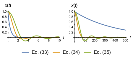
Figure 1: Solutions of (1.2) and (1.3) with $\varphi=(1/2)\omega^{2}x^{2}$. For constant damping (2.21) we choose $\eta$ slightly below the critical value, and for decaying damping (2.22) we choose $r=3$. (a) $\omega=1.5$. (b) $\omega=0.05$.

We illustrate the above solutions in Fig. 1. Note that when $\omega>1$ the gradient flow tends to converge faster to equilibrium, however when $\omega<1$ there is a significant faster convergence of the accelerated gradient flow in both cases. In particular, the oscillations can be better controlled with a constant damping.

The continuous-time dynamics is often easier to analyze compared to the potentially complicated recurrence relations of a discrete-time algorithm. Thus, knowing the behavior of systems (1.2) and (1.3) provide useful insights to understand and design “good” optimization methods. We expect that reasonable discretizations of these systems will reproduce their behavior, at least for sufficiently small choices of the step size. More precisely, it is a general result in numerical analysis [29] that if $\nabla\varphi$ is Lipschitz continuous with constant $L$, a numerical integrator of order $p\geq 1$ has global error $e_{k}\equiv x(t_{k})-x_{k}$ such that $\|e_{k}\|\leq C_{t}h^{p}$, where $t_{k}=kh$ and $C_{t}=C(e^{Lt}-1)$ for some constant $C>0$. Thus, given a fixed simulation time $t$, one can control $e_{k}$ by making the step size $h$ sufficiently small. For our purposes, the dissipative system presumably converges to a minimum of $\varphi$ fast enough, thus we expect that the simulation time will not be excessively large which helps controlling $C_{t}$—this is a better scenario compared to long-time simulations of conservative systems which are common, e.g., in molecular dynamics and astrophysics. Moreover, this estimate on $C_{t}$ is general and pessimistic; a particular method may have a much smaller $C_{t}$. In the following sections we will show that several well-known—but also new—optimization methods are actually discretizations of the gradient flow (1.2) or the accelerated gradient flow (1.3).

4 Accelerated extensions of ADMM

4.1 Balanced and rebalanced splitting

Before making connections with ADMM we need to introduce some ideas about splitting methods for ODEs. Thus, consider the dynamical system

$$\dot{x}=A(x),\qquad A\equiv A_{1}+A_{2},$$ (4.1)

where $A_{1},A_{2}$ represent smooth and single-valued vector fields. Suppose this is an intractable problem, i.e., the structure of $\varphi$ makes the problem not amenable to a numerical procedure. We denote the flow of (4.1) by $\Phi_{t}$. The idea is to split the vector field $A$ such that each individual system

$$\dot{x}=A_{1}(x),\qquad\dot{x}=A_{2}(x),$$ (4.2)

is integrable or has a feasible numerical approximation. We denote their respective flows by $\Phi_{1,t}$ and $\Phi_{2,t}$. For a step size $h>0$, it can be shown [29] that the simplest composition

$$\hat{\Phi}_{h}=\Phi_{2,h}\circ\Phi_{1,h}$$ (4.3)

yields a first-order approximation, namely the local error is $\|\Phi_{h}(x)-\hat{\Phi}_{h}(x)\|=\mathcal{O}(h^{2})$—see Fig. 2a for an illustration. However, in general, splittings such as (4.2) do not preserve critical points of the original ODE. The proposal of [26] is to introduce a balance coefficient, $c=c(t)$, and replace (4.2) by

$$\dot{x}=A_{1}(x)+c,\qquad\dot{x}=A_{2}(x)-c.$$ (4.4)

By appropriately choosing $c$ we can then preserve critical points. To see this, first suppose that $x_{\infty}$ is a critical point of (4.1), i.e., $A_{1}(x_{\infty})+A_{2}(x_{\infty})=0$. If $c_{\infty}$ obeys

$$c_{\infty}=\dfrac{1}{2}\big{(}A_{2}(x_{\infty})-A_{1}(x_{\infty})\big{)}$$ (4.5)

then $x_{\infty}$ is also a critical point of both individual Eqs. (4.4). Conversely, suppose $x_{\infty}$ is a critical point of both individual Eqs. (4.4). We then have

$$\begin{split}c_{\infty}&=A_{2}(x_{\infty})\\ &=-A_{1}(x_{\infty})\\ &=\dfrac{1}{2}\big{(}A_{2}(x_{\infty})-A_{1}(x_{\infty})\big{)},\end{split}$$ (4.6)

implying that $x_{\infty}$ is also a critical point of the original system (4.1). This can be implemented with $c_{k+1}=\tfrac{1}{2}\big{(}A_{2}(x_{k})-A_{1}(x_{k})\big{)}$, together with suitable discretizations of Eqs. (4.4)—see Fig. 2b for an illustration. However, this approach requires explicit computation of the vector fields $A_{i}$’s. In optimization this means computing gradients, which may not be available. To address this issue we consider a related approach.

Figure 2: (a) Splitting approach (4.3). In one time step the error between the continuous and discrete trajectory is $\|x(t_{k+1})-x_{k+1}\|=\mathcal{O}(h^{2})$. (b) The (re)balanced splitting introduces $c_{k}$ which forces the discrete-time evolution to converge to a critical point of the ODE: $\hat{\Phi}_{h}^{k}(x_{0})=\Phi_{t}(x_{0})\to x_{\infty}$ as $k,t\to\infty$.

The rebalanced splitting [26] is particularly well-suited for the implicit discretizations we have in mind. We thus integrate $\dot{x}=A_{1}(x)+c_{k}$ over the interval $[t_{k},t_{k}+h]$, with initial condition $x(t_{k})=x_{k}$, to obtain the intermediate point $x_{k+1/2}$. Then we integrate $\dot{x}=A_{2}(x)-c_{k}$ over the same interval, with initial condition $x(t_{k})=x_{k+1/2}$, to obtain the endpoint $x_{k+1}$. Note that $c_{k}$ is kept fixed during this procedure. Thus,

$$x_{k+1/2} =x_{k}+\int_{t_{k}}^{t_{k}+h}\big{(}A_{1}(x(t))+c_{k}\big{)}dt,$$ (4.7a)

$$x_{k+1} =x_{k+1/2}+\int_{t_{k}}^{t_{k}+h}\big{(}A_{2}(x(t))-c_{k}\big{)}dt.$$ (4.7b)

In light of (4.6), two reasonable ways of computing $c_{k}$ are given by the average of either $\tfrac{1}{2}(A_{2}-A_{1})$ or $A_{2}$. We choose the latter—as we will see this allow us to derive ADMM—which with (4.7) yields

$$\begin{split}c_{k+1}&=\dfrac{1}{h}\int_{t_{k}}^{t_{k}+h}A_{2}(x(t))dt\\ &=c_{k}+h^{-1}\left(x_{k+1}-x_{k+1/2}\right).\end{split}$$ (4.8)

In contrast to the previous case, we now need not compute $A_{i}$ explicitly. Our derivation above is slightly different than the one in Ref. [26].

4.2 Deriving extensions of ADMM

We are now in a position to show how generalizations of ADMM emerge from such an approach. We focus on problem

$$\min_{x\in\mathbb{R}^{n}}\varphi(x),\qquad\varphi=\varphi_{1}+\varphi_{2}+\varphi_{3},$$ (4.9)

and moreover on discretizations of the accelerated gradient flow (1.3) since discretizations of the gradient flow (1.2) can be recovered as particular cases; recall the discussion in Sec. 2.1.

With a balance coefficient $c=c(t)$ we write (1.3) as

$$\dot{x} =p,$$ (4.10a)

$$\dot{p} =\underbrace{-\eta(t)p-\nabla\varphi_{1}(x)-\nabla\varphi_{3}(x)}_{A_{1}}+c\underbrace{-\nabla\varphi_{2}(x)}_{A_{2}}-c.$$ (4.10b)

Splitting as indicated, and further combining the resulting equations, we obtain two independent ODEs:

$$\ddot{x}+\eta(t)\dot{x} =-\nabla\varphi_{1}(x)-\nabla\varphi_{3}(x)+c,$$ (4.11)

$$\ddot{x} =-\nabla\varphi_{2}(x)-c.$$ (4.12)

Using (2.18), and redefining the step size $h^{2}\mapsto h$ as discussed in (2.20), a semi-implicit discretization of (4.11) is

$$\dfrac{x_{k+1/2}-\hat{x}_{k}}{h}=-\nabla\varphi_{1}(x_{k+1/2})-\nabla\varphi_{3}(\hat{x}_{k})+c_{k}.$$ (4.13)

This can be solved with the resolvent (2.1) to obtain

$$x_{k+1/2}=J_{h\partial\varphi_{1}}\big{(}\hat{x}_{k}-h\nabla\varphi_{3}(\hat{x}_{k})+hc_{k}\big{)}.$$ (4.14)

We now discretize (4.12) as

$$\dfrac{\tilde{x}_{k+1}-2x_{k+1/2}+\hat{x}_{k}}{h}=-\nabla\varphi_{2}(x_{k+1})-c_{k}$$ (4.15)

where

$$\tilde{x}_{k+1}\equiv x_{k+1}+(x_{k+1/2}-\hat{x}_{k}).$$ (4.16)

Note that $\tilde{x}_{k+1}$ is related to $x_{k+1}$ via the “momentum” term $(x_{k+1/2}-\hat{x}_{k})$ based on the first splitting. With this and the resolvent we obtain

$$x_{k+1}=J_{h\partial\varphi_{2}}\big{(}x_{k+1/2}-hc_{k}\big{)}.$$ (4.17)

The balance coefficient follows readily from (4.8):

$$c_{k+1}=c_{k}+h^{-1}\left(x_{k+1}-x_{k+1/2}\right).$$ (4.18)

Combining the above steps results into a family of accelerated extensions of ADMM summarized in Algorithm 1.

Choose step size $h$ and damping function $\gamma_{k}$

Initialize $x_{0}$, $\hat{x}_{0}$ and $c_{0}=0$

for $k=0,1,\dotsc$ do

      

      $x_{k+1/2}=\operatorname{prox}_{h\varphi_{1}}\left(\hat{x}_{k}-h\nabla\varphi_{3}(\hat{x}_{k})+hc_{k}\right)$

       $x_{k+1}=\operatorname{prox}_{h\varphi_{2}}(x_{k+1/2}-hc_{k})$

       $c_{k+1}=c_{k}+h^{-1}\left(x_{k+1}-x_{k+1/2}\right)$

       $\hat{x}_{k+1}=x_{k+1}+\gamma_{k+1}(x_{k+1}-x_{k})$

      

end for

Algorithm 1 Family of accelerated extensions of ADMM for problem (4.9).

Let us stress some important aspects of Algorithm 1. The standard ADMM [4, 3, 5] corresponds to the particular case where $\varphi_{3}=0$ and no acceleration is used, i.e., $\gamma_{k}=0$. Thus, Algorithm 1 not only generalizes ADMM to handle problems in the form (4.9) but also includes acceleration with arbitrary damping functions $\eta(t)$. The so-called dual vector in ADMM, originally obtained as a Lagrange multiplier [5], is here represented by the balance coefficient $c_{k}$ and thus acquires a new meaning: its role is to preserve critical points of the ODE.

When decaying damping (2.22) is chosen and $\varphi_{3}=0$, Algorithm 1 is similar to the so-called “fast ADMM” [30]. They differ in that the latter also “accelerates” the dual variable $c_{k}$. Connections between fast ADMM and ODEs was considered recently by us in Refs. [27, 28] and also corresponds to Eq. (1.3), however the discretization is not a rebalanced splitting within the above framework.

In light of the discussion in Sec. 2, it is clear that Algorithm 1 can be generalized to account for monotone operators by the replacements $\operatorname{prox}_{h\varphi_{1}}\to J_{hA_{1}}$ and $\operatorname{prox}_{h\varphi_{2}}\to J_{hA_{2}}$.

Finally, although we focused on the accelerated gradient flow (1.3), analogous procedure applies to the gradient flow (1.2) and leads to Algorithm 1 with $\gamma_{k}=0$.

4.3 Order of accuracy

Next, we show that the above discretization is justified since it is a first-order approximation to the continuous trajectory, i.e., $\|\Phi_{h}(x)-\hat{\Phi}_{h}(x)\|=\mathcal{O}(h^{2})$. From the definition of the resolvent (2.1) we have that $y=J_{h\nabla\varphi}(x)$ if and only if $y=x-h\nabla\varphi(y)$, thus

$$y=x-h\nabla\varphi(x-h\nabla\varphi(y))=x-h\nabla\varphi(x)+\mathcal{O}(h^{2}).$$ (4.19)

This relation implies the following approximations, valid up to $\mathcal{O}(h^{2})$, for the updates in Algorithm 1:

$$x_{k+1/2} \approx\hat{x}_{k}-h\nabla\varphi_{3}(\hat{x}_{k})+hc_{k}-h\nabla\varphi_{1}(\hat{x}_{k}),$$ (4.20)

$$x_{k+1} \approx\hat{x}_{k}-h\nabla\varphi(\hat{x}_{k}).$$ (4.21)

Recall (2.17), namely $\gamma_{k}=1-\sqrt{h}\eta(t_{k})$ since we redefined $h^{2}\mapsto h$. Thus,

$$\hat{x}_{k}=x_{k}+\big{(}1-\eta(t_{k})\sqrt{h}\big{)}\sqrt{h}p_{k}$$ (4.22)

where

$$p_{k}\equiv\dfrac{x_{k}-x_{k-1}}{\sqrt{h}}.$$ (4.23)

From (4.22) and (4.21), and now restoring the original step size ($h\mapsto h^{2}$), we conclude that

$$p_{k+1} \approx p_{k}-h\eta(t_{k})p_{k}-h\nabla\varphi(x_{k}),$$ (4.24)

$$x_{k+1} =x_{k}+hp_{k+1}\approx x_{k}+hp_{k}.$$ (4.25)

Finally, the evolution of Eq. (1.3) in one time step gives

$$p(t+h) =p(t)+h\dot{p}(t)+\mathcal{O}(h^{2})$$

$$\approx p(t)-h\eta(t)p(t)-h\nabla\varphi(x(t)),$$ (4.26)

$$x(t+h) =x(t)+h\dot{x}(t)+\mathcal{O}(h^{2})$$

$$\approx x(t)+hp(t).$$ (4.27)

Comparing with (4.24)–(4.25) implies that the algorithm’s state simulates the continuous trajectory up to an error $\mathcal{O}(h^{2})$, therefore the discretization is first-order accurate. Similar conclusion holds for the nonaccelerated algorithm in relation to the gradient flow (1.2).

We mention a subtlety when $\varphi$ is nonsmooth, or when considering monotone operators more generally. A crucial step in the above derivation was the Taylor approximation of the resolvent (4.19). For a maximal monotone operator $A$, in the most general case only a slightly weaker approximation is available [15, Remark 23.47]:

$$J_{hA}=I-hA_{0}+\mathchoice{{\scriptstyle\mathcal{O}}}{{\scriptstyle\mathcal{O}}}{{\scriptscriptstyle\mathcal{O}}}{\scalebox{0.7}{$\scriptscriptstyle\mathcal{O}$}}(h)$$ (4.28)

where $A_{0}x=\lim_{\mu\downarrow 0}A_{\mu}x$ (see Sec. 2). The previous arguments still hold true, however due to (4.28), and assuming that we can expand $A_{0}(x+\mathcal{O}(h))=A_{0}(x)+\mathcal{O}(h)$, the local error is now $\mathchoice{{\scriptstyle\mathcal{O}}}{{\scriptstyle\mathcal{O}}}{{\scriptscriptstyle\mathcal{O}}}{\scalebox{0.7}{$\scriptscriptstyle\mathcal{O}$}}(h)$ instead of $\mathcal{O}(h^{2})$. It is important to note that this is a consequence of the nonsmoothness of $\varphi$, or the multivaluedness of $A$, and not of the discretization procedure. This comment applies to all cases considered in this paper.

5 Accelerated extensions of Davis-Yin

5.1 Discretization

We now introduce accelerated extensions of Davis-Yin [8]. This time we split the system (1.3) without a balance coefficient, namely we choose vector fields

$$A_{1}(x) =-\eta(t)\dot{x}-\nabla\varphi_{1}(x),$$ (5.1)

$$A_{2}(x) =-\nabla\varphi_{2}(x)-\nabla\varphi_{3}(x).$$ (5.2)

Instead of Eqs. (4.11) and (4.12) we now obtain

$$\ddot{x}+\eta(t)\dot{x} =-\nabla\varphi_{1}(x),$$ (5.3)

$$\ddot{x} =-\nabla\varphi_{2}(x)-\nabla\varphi_{3}(x).$$ (5.4)

Using (2.18) (and redefining $h^{2}\mapsto h$), an implicit discretization of Eq. (5.3) is

$$\dfrac{x_{k+1/4}-\hat{x}_{k}}{h}=-\nabla\varphi_{1}(x_{k+1/4}),$$ (5.5)

which with the resolvent (2.1) gives

$$x_{k+1/4}\equiv\Phi_{1,h}(\hat{x}_{k})=J_{h\partial\varphi_{1}}(\hat{x}_{k}).$$ (5.6)

Next, to “inject momentum” in the direction of $\nabla\varphi_{1}$, we define the “translation operator”

$$\mathcal{T}_{h}(z)\equiv z-h\nabla\varphi_{1}(x_{k+1/4}).$$ (5.7)

The next point is thus obtained as

$$x_{k+1/2}\equiv\mathcal{T}_{h}(x_{k+1/4})=2x_{k+1/4}-\hat{x}_{k}.$$ (5.8)

A semi-implicit discretization of Eq. (5.4) is

$$\dfrac{x_{k+3/4}-2x_{k+1/4}+\hat{x}_{k}}{h}=-\nabla\varphi_{2}(x_{k+3/4})-\nabla\varphi_{3}(x_{k+1/4}),$$ (5.9)

which can again be solved with the resolvent (2.1) to obtain

$$\begin{split}x_{k+3/4}&\equiv\Phi_{2,h}(\hat{x}_{k})\\ &=J_{h\partial\varphi_{2}}\left(x_{k+1/2}-h\nabla\varphi_{3}(x_{k+1/4})\right).\end{split}$$ (5.10)

Finally, applying the inverse $\mathcal{T}^{-1}_{h}(z)\equiv z+h\nabla\varphi_{1}(x_{k+1/4})$ and using (5.5) we obtain

$$x_{k+1}\equiv\mathcal{T}^{-1}_{h}(x_{k+3/4})=x_{k+3/4}-(x_{k+1/4}-\hat{x}_{k}).$$ (5.11)

We collect the above steps into Algorithm 2. The original Davis-Yin method [8] is recovered by setting $\gamma_{k}=0$. Such a case corresponds to an overdamped limit—recall the discussion of Sec. 2.1—which is indeed a discretization of the gradient flow (1.2), as can also be easily verified by repeating the above procedure to this simpler case.

Choose step size $h$ and damping function $\gamma_{k}$

Initialize $x_{0}$ and $\hat{x}_{0}$

for $k=0,1,\dotsc$ do

      

      $x_{k+1/4}=\operatorname{prox}_{h\varphi_{1}}(\hat{x}_{k})$

       $x_{k+1/2}=2x_{k+1/4}-\hat{x}_{k}$

       $x_{k+3/4}=\operatorname{prox}_{h\varphi_{2}}\big{(}x_{k+1/2}-h\nabla\varphi_{3}(x_{k+1/4})\big{)}$

       $x_{k+1}=\hat{x}_{k}+x_{k+3/4}-x_{k+1/4}$

       $\hat{x}_{k+1}=x_{k+1}+\gamma_{k+1}(x_{k+1}-x_{k})$

      

end for

Algorithm 2 Family of accelerated extensions of Davis-Yin (DY) for problem (4.9).

Algorithm 2 is equivalent to the fixed point iteration $x_{k+1}=\hat{\Phi}_{h}(\hat{x}_{k})$ with

$$\hat{\Phi}_{h}\equiv\mathcal{T}^{-1}_{h}\circ\Phi_{2,h}\circ\mathcal{T}_{h}\circ\Phi_{1,h},$$ (5.12)

where these individual maps are defined in Eqs. (5.6), (5.7), and (5.10). Thus, the translation operator $\mathcal{T}_{h}$ is actually a “preprocessor map,” which is a common technique in numerical analysis [29]. The discretization associated to Davis-Yin can be summarized diagrammatically:

(5.13)

5.2 Order of accuracy

Using the expansion (4.19) we can approximate the updates of Algorithm 2 up to $\mathcal{O}(h^{2})$:

$$x_{k+1/4} \approx\hat{x}_{k}-h\nabla\varphi_{1}(\hat{x}_{k}),$$ (5.14a)

$$x_{k+1/2} \approx\hat{x}_{k}-2h\nabla\varphi_{1}(\hat{x}_{k}),$$ (5.14b)

$$x_{k+3/4} \approx\hat{x}_{k}-2h\nabla\varphi(\hat{x}_{k}),$$ (5.14c)

$$x_{k+1} \approx\hat{x}_{k}-h\nabla\varphi(\hat{x}_{k}).$$ (5.14d)

But (5.14d) is exactly the same as (4.21), thus the remaining steps of the argument follow as before, implying that Algorithm 2 is also a first-order integrator to the accelerated gradient flow (1.3). The same holds true for standard Davis-Yin ($\gamma_{k}=0$) in relation to the gradient flow (1.2).

5.3 Preserving critical points

Since Algorithm 2 arises from a splitting that is not balanced, it is not a priori obvious if critical points of the underlying ODE are preserved. We now show that this is indeed the case. We can write the operator (5.12) as

$$\hat{\Phi}_{h}=I+J_{h\partial\varphi_{2}}\circ\left(2J_{h\partial\varphi_{1}}-I-h\nabla\varphi_{3}\circ J_{h\partial\varphi_{1}}\right)-J_{h\partial\varphi_{1}}.$$ (5.15)

Assuming the algorithm converges, we must have a fixed point equation $x_{\infty}=\hat{\Phi}_{h}(x_{\infty})$. We thus need to show that this equation generates critical points of the ODE. To this end, let $x^{\star}$ be such a critical point, i.e.,

$$(\nabla\varphi_{1}+\nabla\varphi_{2}+\nabla\varphi_{3})(x^{\star})=0.$$ (5.16)

This is equivalent to $(I+h\nabla\varphi_{2})(x^{\star})=(I-h\nabla\varphi_{1}-h\nabla\varphi_{3})(x^{\star})$, and with the aid of the resolvent (2.1) it can be written as

$$x^{\star}=J_{h\partial\varphi_{2}}\circ(I-h\nabla\varphi_{1}-h\nabla\varphi_{3})(x^{\star}).$$ (5.17)

Using the identity

$$(2J_{h\partial\varphi}-I)\circ(I+h\nabla\varphi)=I-h\nabla\varphi$$ (5.18)

we thus have

$$x^{\star}=J_{h\partial\varphi_{2}}\circ\left[(2J_{h\partial\varphi_{1}}-I)\circ(I+h\nabla\varphi_{1})-h\nabla\varphi_{3}\right](x^{\star}).$$ (5.19)

Define $x_{\infty}\equiv(I+h\nabla\varphi_{1})(x^{\star})$, i.e., $x^{\star}=J_{h\partial\varphi_{1}}(x_{\infty})$. The above equation then yields

$$J_{h\partial\varphi_{1}}(x_{\infty})=J_{h\partial\varphi_{2}}\circ\left[2J_{h\partial\varphi_{1}}-I-h\nabla\varphi_{3}\circ J_{h\partial\varphi_{1}}\right](x_{\infty})$$ (5.20)

which is equivalent to $x_{\infty}=\hat{\Phi}_{h}(x_{\infty})$ according to (5.15). Therefore, critical points of (5.16) yield fixed points of the operator (5.15) and vice-versa. This shows that Algorithm 2 preserves critical points of the underlying ODE.

5.4 Accelerated extensions of Douglas-Rachford

Douglas-Rachford (DR) [2, 6] is recovered from Algorithm 2 in the particular case where $\gamma_{k}=0$ and $\varphi_{3}=0$. Therefore, in the case where $\varphi_{3}=0$ but $\gamma_{k}\neq 0$, Algorithm 2 contains accelerated extensions of Douglas-Rachford—the case with decaying damping was considered in [31]. From the previous arguments, we know that such methods are discretizations of the accelerated gradient flow (1.3), whereas the standard Douglas-Rachford is a discretization of the gradient flow (1.2). Moreover, such discretizations preserve critical points and are first-order integrators.

5.5 Accelerated extensions of forward-backward

The forward-backward method [6] is recovered from Algorithm 2 when $\gamma_{k}=0$ and $\varphi_{1}=0$. Thus, when $\varphi_{1}=0$ but $\gamma_{k}\neq 0$, Algorithm 2 reduces to

$$\begin{split}x_{k+1}&=\operatorname{prox}_{h\varphi_{2}}\big{(}\hat{x}_{k}-h\nabla\varphi_{3}(\hat{x}_{k})\big{)},\\ \hat{x}_{k+1}&=x_{k+1}+\gamma_{k+1}(x_{k+1}-x_{k}).\end{split}$$ (5.21)

The decaying damping case (2.22) was considered in [32]. From an ODE perspective, the above discretization is not a splitting method but rather a direct semi-implicit discretization of Eq. (1.3). Anyhow, our previous arguments show that such accelerated variants of forward-backward are first-order integrators of this ODE and preserve critical points—the same holds true for the standard forward-backward ($\gamma_{k}=0$) in relation to the gradient flow (1.2).

6 Accelerated extensions of Tseng’s splitting

The last proximal method remaining to be considered is the forward-backward-forward or Tseng’s splitting [7]. Thus, consider Eq. (1.3) with $\varphi_{1}=0$ and written as

$$\dot{p} =\underbrace{-\eta(t)p-\nabla\varphi_{2}(x)-\nabla\varphi_{3}(x)}_{A_{1}}+\underbrace{\nabla\varphi_{3}(x)-\nabla\varphi_{3}(x)}_{A_{2}}.$$ (6.1)

Note that $A_{2}=0$, however in a discretization there might be numerical inaccuracies which introduces a kind of “perturbation” on top of the forward-backward method, which arises from the first component of this system. Splitting as indicated yields

$$\ddot{x}+\eta(t)\dot{x} =-\nabla\varphi_{2}(x)-\nabla\varphi_{3}(x),$$ (6.2)

$$\ddot{x} =\nabla\varphi_{3}(x)-\nabla\varphi_{3}(x).$$ (6.3)

A semi-implicit discretization of the first equation yields

$$x_{k+1/2}=J_{h\partial\varphi_{2}}\left(\hat{x}_{k}-h\nabla\varphi_{3}(\hat{x}_{k})\right),$$ (6.4)

which is the forward-backward method (5.21). Eq. (6.3) can be discretized as $\tilde{x}_{k+1}-2x_{k+1/2}+\hat{x}_{k}=h\nabla\varphi_{3}(\hat{x}_{k})-h\nabla\varphi_{3}(x_{k+1/2})$, where $\tilde{x}_{k+1}$ is given by (4.16). Thus,

$$x_{k+1}=x_{k+1/2}-h\big{(}\nabla\varphi_{3}(x_{k+1/2})-\nabla\varphi_{3}(\hat{x}_{k})\big{)}.$$ (6.5)

Therefore, we derived Algorithm 3.

Choose step size $h$ and damping function $\gamma_{k}$

Initialize $x_{0}$ and $\hat{x}_{0}$

for $k=0,1,\dotsc$ do

      

      $x_{k+1/2}=\operatorname{prox}_{h\varphi_{2}}\left(\hat{x}_{k}-h\nabla\varphi_{3}(\hat{x}_{k})\right)$

       $x_{k+1}=x_{k+1/2}-h\left(\nabla\varphi_{3}(x_{k+1/2})-\nabla\varphi_{3}(\hat{x}_{k})\right)$

       $\hat{x}_{k+1}=x_{k+1}+\gamma_{k+1}(x_{k+1}-x_{k})$

      

end for

Algorithm 3 Family of accelerated extensions of Tseng’s method.

The original Tseng’s splitting is recovered with $\gamma_{k}=0$, in which case it is a discretization of the gradient flow (1.2). Due to Eq. (6.3) we expect to have a “contraction” on the acceleration which indicates that Algorithm 3 may be slower than (5.21) (this was actually observed in our experiments and this method tends to be slower than forward-backward).

In a similar way as already done in Secs. 4 and 5, through Taylor expansions it is straightforward to show that the above discretization is first-order accurate.

We can also show that the above discretization preserves critical points. Indeed, Algorithm 3 is equivalent to iterations $x_{k+1}=\hat{\Phi}_{h}(\hat{x}_{k})$ with

$$\hat{\Phi}_{h}=(I-h\nabla\varphi_{3})\circ J_{h\partial\varphi_{2}}\circ(I-h\nabla\varphi_{3})+h\nabla\varphi_{3}.$$ (6.6)

Assuming the algorithm converges, $x_{\infty}=\hat{\Phi}_{h}(x_{\infty})$, i.e.,

$$(I-h\nabla\varphi_{3})(x_{\infty})=(I-h\nabla\varphi_{3})\circ J_{h\partial\varphi_{2}}\circ(I-h\nabla\varphi_{3})(x_{\infty}).$$ (6.7)

Moreover, assuming that $h$ is sufficiently small so that the inverse $(I-h\nabla\varphi_{3})^{-1}$ exists, the above yields $x_{\infty}=J_{h\partial\varphi_{2}}\circ(I-h\nabla\varphi_{3})(x_{\infty})$. By the definition of resolvent in Eq. (2.1) this is equivalent to $\nabla(\varphi_{2}+\varphi_{3})(x_{\infty})=0$. Thus, the iterates of this algorithm generates critical points of the underlying ODE.

7 A classical view on deterministic optimization

Figure 3: Several well-known optimization methods arise as dicretizations of the gradient flow. Moreover, “accelerated extensions” of these methods arise as discretizations of Newton’s equation with a dissipative term; the gradient flow corresponds to a large friction limit of the latter. Therefore, these optimization methods consist of actual simulations of a classical dissipative physical system.

At this stage, let us summarize and interpret the previous results from a physics perspective. They can be summarized by Fig. 3. Several well-known optimization methods—including gradient- or proximal-based—are simply different discretizations of the gradient flow. This includes gradient descent (see the Appendix), forward-backward, Tseng’s splitting, ADMM, Douglas-Rachford, Davis-Yin, and potentially many other methods. However, accelerated extensions of these methods arise as discretizations of Newton’s equation with a dissipative term. Besides the accelerated proximal methods we introduced, we also have Nesterov and heavy ball (see the Appendix and Ref. [21]), and potentially many others as well. All these methods are provably first-order integrators, i.e., they have a local error $\mathcal{O}(h^{2})$, and preserve critical points of the associated ODE. In addition, let us mention that we have recently generalized symplectic integrators to general dissipative Hamiltonian systems [33], which may offer a systematic approach to construct gradient-based optimization methods. Therefore, all these optimization methods can be seen as actual simulations of a classical dissipative system; when someone solves an optimization problem by implementing one of these methods in a—presumably classical—computer, there is a simulation of one classical system, i.e., dissipative Newton’s equation, by another classical system, i.e., the computer.

There are many interesting open questions even at this classical level. For instance, given a potential $\varphi:\mathbb{R}^{n}\to\mathbb{R}$ where certain properties of its landscape are known, is there a lower bound on how fast a dissipative system can approach the ground state? If so, which specific system would achieve such rate of convergence? Given $\varphi$, what is the best way to dissipate energy, i.e., the best damping $\eta(t)$? What is the tradeoff between energy dissipation and stability? Answering these type of questions would allow us to design “optimal” optimization algorithms through suitable discretizations of dissipative physical systems.

A dissipative Newtonian system is deterministic, and so are the optimization methods obtained as its discretizations. Such a deterministic approach is suited to convex problems which have a unique global minimum, or to obtain local minima in the neighborhood of the initial state. However, to escape poor local minima in more complex landscapes, i.e., to solve more challenging nonconvex problems, we need to introduce some sort of perturbation or noise. Thus, in the next section, we will generalize these methods to stochastic optimization settings. This will allow us to make connections with Langevin and Fokker-Planck equations which are ubiquitous in nonequilibrium statistical mechanics. It is worth noticing that such an approach is in some sense more closely related to sampling than to pure or deterministic optimization.

8 Stochastic optimization

8.1 Stochastic gradient

One of the motivations behind stochastic optimization is to lighten the computational burden in computing full gradients over entire datasets, which is a bottleneck for high-dimensional problems with large data. The basic idea dates back to Robbins and Monro [34] and nowadays is widely used in machine learning, especially in training neural networks. Consider replacing the deterministic problem (1.1) by its stochastic counterpart

$$\min_{x\in\mathbb{R}^{n}}\mathbb{E}_{\omega}[\ell(x;\omega)],$$ (8.1)

where $\omega$ is a random variable from a sample space $\Omega$. Specifically, suppose we have training data $\{\omega_{1},\dotsc,\omega_{N}\}$ so that $\ell_{i}(x)\equiv\ell(x;\omega_{i})$ is a random variable. Numerically, the above expectation is approximated by the empirical mean,

$$\overline{\ell}(x)\equiv\dfrac{1}{N}\sum_{i=1}^{N}\ell_{i}(x),$$ (8.2)

which is exact when $N\to\infty$. Thus, instead of computing $\overline{\nabla\ell}(x)=\tfrac{1}{N}\sum_{i=1}^{N}\nabla\ell_{i}(x)$ that may not be feasible, at each iteration of the algorithm we sample a “minibatch” $\mathcal{B}$, of size $S$, drawn uniformly at random—without replacement—from an index set $\{1,\dotsc,N\}$ and compute the so-called stochastic gradient

$$\widetilde{\nabla\ell}(x)\equiv\dfrac{1}{S}\sum_{i\in\mathcal{B}}\nabla\ell_{i}(x).$$ (8.3)

Note that when $S=N$ this becomes the true gradient of the empirical loss (8.2). Importantly, when the dataset is very large, i.e., $S\ll N$ and $N\to\infty$, the central limit theorem comes into play and

$$\widetilde{\nabla\ell}(x)=\overline{\nabla\ell}(x)+\xi(x)$$ (8.4)

where $\xi(x)\sim\mathcal{N}\big{(}0,\Sigma(x)\big{)}$. Thus, the stochastic gradient is an unbiased estimator of the true gradient of the empirical loss. It is reasonable to assume that the covariance matrix takes the form

$$\Sigma(x)=\dfrac{1}{S}C(x)C^{T}(x)$$ (8.5)

for some matrix $C(x)$. We do not know the specific form of $C(x)$, which is data dependent, however in principle it can be estimated. When $N,S\to\infty$, but with the ratio $S/N\ll 1$ kept fixed, we have $\Sigma\to 0$ and the stochastic gradient becomes the gradient of the expectation in problem (8.1)—this can be seen as a thermodynamic limit.

The stochastic gradient (8.3) can be implemented into the previous algorithms quite easily. Since $\varphi_{3}$ is the only function assumed to be differentiable in problem (4.9), we consider

$$\min_{x\in\mathbb{R}^{n}}\,\varphi_{1}(x)+\varphi_{2}(x)+\mathbb{E}_{\omega}[\varphi_{3}(x;\omega)].$$ (8.6)

The entire family of Algorithms 1, 2 and 3 can be adapted to such case by adding two simple steps at each iteration, i.e., in the very first line of the “for” loop:

1. Sample a minibatch $\mathcal{B}\subset\{1,\dotsc,N\}$ of size $S$ uniformly at random and without replacement;

2. Replace $\nabla\varphi_{3}\to\widetilde{\nabla\varphi}_{3}$ in the subsequent updates.

8.2 Stochastic proximal operator

We can use similar ideas for proximal operators. As before, in each iteration of the algorithm we sample a minibatch $\mathcal{B}$ and define

$$\widetilde{\ell}(x)\equiv\dfrac{1}{S}\sum_{i\in\mathcal{B}}\ell_{i}(x),\qquad\ell_{i}\equiv\ell(x,\omega_{i}).$$ (8.7)

Thus, at each iteration, the algorithm has access to a random function $\widetilde{\ell}(x)$ that presumably “mimics” $\mathbb{E}_{\omega}[\ell(x;\omega)]$. We replace the proximal operator of the empirical loss, $\operatorname{prox}_{h\overline{\ell}}(x)$, by its stochastic counterpart

$$\begin{split}\widetilde{\operatorname{prox}}_{h\ell}(x)&\equiv\operatorname{prox}_{h\widetilde{\ell}}(x)\\ &=\operatorname*{arg\,min}_{y}\left(\widetilde{\ell}(y)-\dfrac{1}{2h}\|y-x\|^{2}\right).\end{split}$$ (8.8)

Suppose we introduce stochasticity through $\varphi_{2}$ in problem (4.9), i.e.,

$$\min_{x\in\mathbb{R}^{n}}\,\varphi_{1}(x)+\mathbb{E}_{\omega}[\varphi_{2}(x;\omega)]+\varphi_{3}(x).$$ (8.9)

Then the family of Algorithms 1, 2 and 3 are adapted by adding the following instructions at each iteration:

1. Sample a minibatch $\mathcal{B}\subset\{1,\dotsc,S\}$ of size $S$ uniformly at random and without replacement;

2. Replace $\operatorname{prox}_{h\varphi_{2}}\to\widetilde{\operatorname{prox}}_{h\varphi_{2}}$ in the next updates.

Note that, also in this case, a similar relation to (8.4) holds. Indeed, from (4.19) we get

$$\begin{split}\widetilde{\operatorname{prox}}_{h\ell}(x)&\approx x-h\widetilde{\nabla\ell}(x)\\ &=x-h\overline{\nabla\ell}(x)+h\xi(x)\\ &\approx\operatorname{prox}_{h\overline{\ell}}(x)+h\xi(x).\end{split}$$ (8.10)

8.3 Langevin and Fokker-Planck equations

In the deterministic case we have the situation depicted in Fig. 3. In light of the discussion above, introducing a stochastic gradient or a stochastic proximal operator into these methods is equivalent to introducing a random perturbation in the associated ODEs. Thus, the only difference compared to the deterministic case is that $\nabla\varphi(x)$ is replaced by a “stochastic gradient,” $\widetilde{\nabla\varphi}(x)$, during a time interval of one step size $h$. As a consequence of Eqs. (8.4) and (8.10), we can describe this process by a Brownian motion provided we account for the correct power of the step size $h$ when discretizing the noise term. Therefore, we must choose

$$\sqrt{\dfrac{h}{S}}C(x)dW\to\sqrt{\dfrac{h}{S}}C(x_{k})\sqrt{h}\,\epsilon_{k}\equiv h\xi(x_{k})$$ (8.11)

where $W$ is a standard Wiener process, $\epsilon_{k}\sim\mathcal{N}(0,I)$, and $\xi(x)$ is the noise of the stochastic gradient (8.4), or the noise of the stochastic proximal operator (8.10). The gradient flow (1.2) is thus replaced by the overdamped Langevin equation

$$dx=-\nabla\varphi(x)dt+\sqrt{\dfrac{h}{S}}C(x)dW.$$ (8.12)

Similarly, the accelerated gradient flow (1.3) is replaced by the underdamped Langevin equation

$$dx =pdt,$$ (8.13a)

$$dp =-\nabla\varphi(x)dt-\eta(t)pdt+\sqrt{\dfrac{h}{S}}C(x)dW.$$ (8.13b)

There is one subtle point about these SDEs. They have a multiplicative white noise which is often ambiguous, e.g., the Itô-Stratonovich dilemma. In our context, it should be noted that the stochastic versions of the proximal methods previously discussed can be obtained from these SDEs as long as we discretize the noise consistently with the gradient of either $\nabla\varphi_{3}$ or $\nabla\varphi_{2}$, i.e., the previous splitting schemes must be followed carefully by discretizing $C(x)$ appropriately so that we can combine the noise into the stochastic gradient $\widetilde{\nabla\varphi_{3}}$—in the case of (8.6)—or the stochastic proximal operator $\widetilde{\operatorname{prox}}_{h\varphi_{2}}$—in the case of (8.9). Naturally, there is no ambiguity if we assume additive noise, i.e., constant $C$, which should already provide insights into these methods, at least qualitatively.

We should also point out that stochastic versions of gradient descent, Polyak’s heavy ball, and Nesterov—which are gradient-based methods and widely used in machine learning—also follow from this approach. In these cases the discretization is explicit, i.e., one has a single gradient, no splitting, and no proximal operators. Moreover, the noise term is discretized in the Itô sense. For instance, stochastic gradient descent is simply an Euler-Maruyama discretization of (8.12). The stochastic version of Nesterov arises similarly from (8.13) by using (2.18). For heavy ball, one should use a “conformal symplectic integrator” for the deterministic part of (8.13)—see Ref. [21]—and compose with an Itô discretization of the noise; we provide these derivations in the Appendix for completeness.

An interesting aspect of the above SDEs is that the ratio $h/S$ plays the role of an “effective temperature” $T$. This is intuitive: small $S$ means more noise in the stochastic gradient approximation, which is equivalent to raising the temperature of the heat bath, while increasing the step size simply amplifies the noise. The limit $S\to\infty$—which presumes $N\to\infty$ and $S/N\ll 1$—corresponds to removing the heat bath so that the previous SDEs together with their discretizations become deterministic. In similar vein as discussed in Sec. 2.1, the Langevin equation (8.12) can be recovered from (8.13) in the large friction limit. Therefore, the overall picture relating all possible variants of these optimization methods is depicted in Fig. 4; depending from which “quadrant” one chooses to discretize, and depending which discretization scheme is chosen, one can obtain an optimization algorithm with qualifiers such as “accelerated,” “stochastic,” or both, or none. The underdamped Langevin (top left quadrant) is the most general model that unifies all methods.

Figure 4: Different optimization algorithms arise from different discretizations (dashed lines) of the same physical system. The left column of the diagram represents stochastic processes described by a Langevin equation, while the right column represents deterministic processes from (dissipative) classical mechanics—the transition between these phases is controlled by the “temperature” $T\sim 1/S$ where $S$ is the batch size. The upper row of the diagram corresponds to an underdamped or accelerated regime, while the lower row corresponds to an overdamped regime where acceleration is negligible—the transition is controlled by the damping coefficient $\eta$. Discretizations from each colored quadrant yield (variants of) optimization algorithms in these “different phases.”

Now, we can readily write down the Fokker-Planck equation associated to the above SDEs, which describe the probability density $P(x,t)$—or $P(x,p,t)$ for the accelerated methods—of the stochastic process. From the Chapman-Kolmogorov equation, through a standard derivation, we find that in the case of (8.12) we have

$$\dfrac{\partial P}{\partial t}=\nabla\cdot(P\nabla\varphi(x))+\Delta_{D}P,$$ (8.14)

where we defined the diffusion matrix and the “stochastic Laplacian” as

$$D\equiv\dfrac{h}{2S}C(x)C(x)^{T},\qquad\Delta_{D}P\equiv\sum_{i,j}\dfrac{\partial^{2}}{\partial x_{i}\partial x_{j}}(D_{ij}P).$$ (8.15)

Similarly, the Fokker-Planck equation associated to the underdamped Langevin (8.13) is given by

$$\dfrac{\partial P}{\partial t}=-\nabla_{x}\cdot\left(pP\right)+\nabla_{p}\cdot\left(P\nabla\varphi(x)+\eta(t)pP\right)+\Delta_{D}P.$$ (8.16)

However, here $\Delta_{D}P=\sum_{ij}D_{ij}(x)\partial_{p_{i}}\partial_{p_{j}}P$ since the noise is coupled only to the momenta.

In Eqs. (8.12) and (8.13) the Brownian motion arises from a stochastic gradient or stochastic proximal operator approximation, hence the diffusion dependence on the minibatch and step sizes. Alternatively, one can directly perturb the deterministic optimization methods with a Gaussian noise. Both situations are conceptually similar except that in the latter case we have discretizations of the usual Langevin dynamics where the Brownian motion is controlled independently by a heat bath. The noise term of Eq. (8.13) is thus replaced by the standard $\sqrt{2D}dW$, which obeys Einstein’s fluctuation-dissipation relation $D=\eta\,k_{B}T$, assuming $\eta=\mbox{const.}$ The overdamped limit yields Eq. (8.12) with the same term but $D=k_{B}T$. In this setting, we have “sampling methods” where the dynamics first relax to equilibrium and then perform random excursions around a local minimum of $\varphi$. From this perspective, the stochastic optimization methods are conceptually closer to a sampling approach, however with smaller and limited control over the noise.

9 Numerical Experiments

9.1 Order of accuracy

We start by illustrating how accurate the previous optimization methods approximate the gradient flow ODEs. We consider Algorithms 1 and 2—recall that the latter reduces to (accelerated versions of) Douglas-Rachford and forward-backward as particular cases, so we are indirectly testing them as well. We compare these methods with the exact solutions (3.7) and (3.8). To this end, we choose a composite function:

$$\varphi=\varphi_{1}+\varphi_{2}+\varphi_{3},\qquad\varphi_{i}(x)=\omega_{i}^{2}x^{2}/2,$$ (9.1)

with $\omega_{1}=1/2$, $\omega_{2}=1/3$ and $\omega_{3}=1/5$—recall that there is splitting of these individual functions in the algorithms. As we can see in Figs. 5a and 5b, these methods closely match the exact solutions. Naturally, for large step sizes there might be significant deviations. However, since these methods were proven to be first-order integrators, they are accurate up to a global error $\mathcal{O}(h)$. To verify this, for a given step size $h$ we compute

$$\max_{k\in[0,K]}|x(t_{k})-x_{k}|$$ (9.2)

for $K=t_{\textnormal{max}}/h$, where $t_{\textnormal{max}}$ is a fixed simulation time (we choose again $t_{\textnormal{max}}=25$). We thus compare this maximum error over the entire history of the system against a range of step sizes. Results for the constant damping case are shown in Fig. 5c—we performed the same simulation with decaying damping but the plot is nearly indistinguishable from this one.

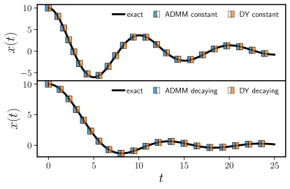
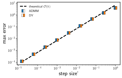
Figure 5: Comparison of the discretization provided by Algorithms 1 and 2 versus the exact solution of the second-order gradient flow (1.3) with (9.1). (a) Constant damping with $\eta=0.2$. (b) Decaying damping with $r=3$. In both cases we chose step size $h=0.01$. (c) Maximum error (9.2) over a range of step sizes. We consider constant damping under the setting of Fig. 5a—similar results hold for decaying damping.

In these experiments there is no visible difference between—accelerated—Davis-Yin and ADMM. This is also explained by our theoretical results since both methods consist of numerical integrators of the same order of accuracy and to the same physical system.

9.2 Langevin approximation

We now wish to verify the Langevin approximation to the stochastic variants of the optimization methods introduced in the previous section. Consider thus a quadratic function as in Eq. (9.1), again with $\omega_{1}=1/2$ and $\omega_{2}=1/3$, but now $\varphi_{3}$ is generated randomly so as to obtain a problem in the form (8.6). We set

$$\varphi_{3}(x)=\dfrac{1}{2N}\sum_{i=1}^{N}\theta_{i}^{2}x^{2}$$ (9.3)

with $\theta_{i}$ sampled uniformly from the interval $[0,1]$. We choose $N=1000$ and $\varphi_{3}$ is kept fixed in all simulations, i.e., we have an “empirical mean” as in (8.2). To obtain stochastic gradients (8.3), at each iteration of Algorithms 1 and 2 we sample a minibatch of $\theta_{i}$’s of size $S=1$—this is the only source of stochasticity. For simplicity, we focus on the nonaccelerated methods ($\gamma_{k}=0$) which are modelled by the overdamped Langevin (8.12). Since the function is quadratic, if we assume a constant $D$ into (8.14)—which we know is not the case but it should already capture the qualitative behavior—we then have an Ornstein-Uhlenbeck process whose probability density, $P(x,t|x_{0},t_{0}=0)$, is given by

$$\sqrt{\dfrac{\lambda}{2\pi D(1-e^{-2\lambda t})}}\exp\left\{-\dfrac{\lambda\left(x-x_{0}e^{-\lambda t}\right)^{2}}{2D(1-e^{-2\lambda t})}\right\},$$ (9.4)

with $\lambda=\omega_{1}^{2}+\omega_{2}^{2}+\tfrac{1}{2N}\sum_{i}^{N}\theta_{i}^{2}$. In our simulations we choose a step size $h=0.1$, maximum time $t_{\textnormal{max}}=10$, and initial position $x_{0}=10$. We consider $2000$ Monte Carlo runs, with $\varphi_{3}$ fixed so that only the minibatch changes in each simulation. In Fig. 6a we show histograms for stochastic ADMM and Davis-Yin for a single time instant ($t=2$). We can see that both methods give essentially the same results and agree with the out-of-equilibrium Gaussian prediction (9.4). Similar results hold for other time instants, as illustrated in Fig. 6b. Here we set $D=4$ to obtain the shaded gray area—this value was estimated with the simulation for $t=1$, and we picked this time since the variance was sufficiently large. We also indicate the standard deviation of both methods (vertical red lines) which actually vary with $x$, however everything is well-described by Eq. (9.4), in agreement with the Langevin approximation. We mention that simulations with other values of the batch and step sizes were also considered, verifying similar results but where the Gaussian approximation is more or less peaked according to the the scaling $h/S$ from Eq. (8.15).

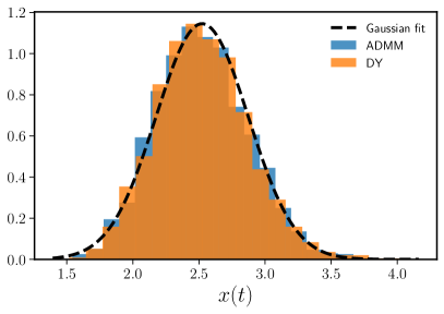
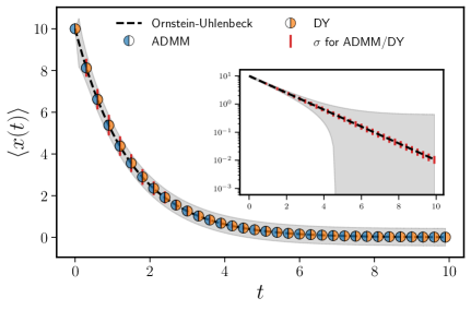
Figure 6: (a) Histogram of stochastic variants of Algorithms 1 and 2 (with $\gamma_{k}=0$) for a quadratic problem which is modelled by an Ornstein-Uhlenbeck process; we considered (9.3) with $N=1000$, minibatch of size $S=1$, step size $h=0.1$, initial position $x_{0}=10$ and $2000$ Monte Carlo runs. We show the simulation for $t=2$. The Gaussian fit has mean $\mu=2.52$ and variance $\sigma=0.35$. The theoretical prediction from Eq. (9.4) is $\mu=2.51$, in close agreement. (b) Same type of simulation for $t\in[0,10]$. The dashed line is the mean of the Ornstein-Uhlenbeck process (9.4), and the shaded area indicates the standard deviation with $D=4$. The markers are the means of ADMM and Davis-Yin, and the vertical red lines are standard deviations for both methods, which are very close. The inset is exactly the same plot but with markers omitted and the $y$-axis on log scale.

9.3 Machine learning experiments

We now wish to verify whether the accelerated methods we introduced are able to achieve faster convergence compared to the base methods, which are the actual known methods in the literature. According to the discussion in Sec. 3, we expect that this might be the case. We focus on two types of damping: constant (2.21), and decaying (2.22). When nothing is specified it means that no acceleration is used, i.e., $\gamma_{k}=0$ in Eq. (2.17), which yields the base methods. We consider ADMM (Algorithm 1), DY (Algorithm 2) and Tseng (Algorithm 3). Forward-backward (FB) is Algorithm 2 with $\varphi_{1}=0$ and Douglas-Rachford (DR) with $\varphi_{3}=0$.

Consider a LASSO regression problem that is of fundamental importance to machine learning and statistics:

$$\min_{x\in\mathbb{R}^{n}}\varphi(x),\qquad\varphi(x)\equiv\dfrac{1}{2}\|Ax-b\|^{2}+\alpha\|x\|_{1},$$ (9.5)

where $A\in\mathbb{R}^{m\times n}$ is a given matrix, $b\in\mathbb{R}^{m}$ is a given signal, and $\alpha>0$ is a coupling constant. Here $\|\cdot\|_{1}$ denotes the $\ell_{1}$-norm, known to induce “sparsity”—this function is not differentiable although its proximal operator has a well-known closed form solution called soft thresholding. Following Ref. [10, Sec. 7.1.3], we generate data by sampling $A_{ij}\sim\mathcal{N}(0,1)$ and then normalize its columns to have unit norm. We sample $x_{\bullet}\in\mathbb{R}^{n}\sim\mathcal{N}(0,1)$ with sparsity level $95\%$ (only $5\%$ of its entries are nonzero) and then add noise to obtain the observed signal $b=Ax_{\bullet}+e$ where $e\sim\mathcal{N}(0,10^{-3})$. We choose dimensions $m=500$ and $n=2500$—the signal-to-noise ratio is $\approx 250$, and $x_{\bullet}$ has $125$ nonzero entries. We set $\alpha=0.1\alpha_{\textnormal{max}}$ where $\alpha_{\textnormal{max}}=\|A^{T}b\|_{\infty}$ is the largest value such that (9.5) admits a nontrivial solution—the factor $0.1$ was verified to yield good results after few trials. We evaluate the algorithms by computing the relative error $|\varphi(x_{k})-\varphi^{\star}|/\varphi^{\star}$ where $\varphi^{\star}$ is the solution obtained with an independent and reliable solver—we use the default implementation of CVXPY which is a standard optimization library in the Python language. For all algorithms, we choose step size $h=0.08$, which is the largest choice such that all algorithms converge. For decaying damping we choose $r=3$ in (2.22)—this choice is standard but we verified that other values did not improve—and for constant damping we choose $\eta=0.5$ in (2.21)—this value was tuned with a rough grid search. In Fig. 7 we report the mean and standard deviation (small error bars) across 10 randomly generated instances of problem (9.5). The figure shows that the accelerated variants of each method improve over the base method. In particular, the constant damping variants are the fastest.

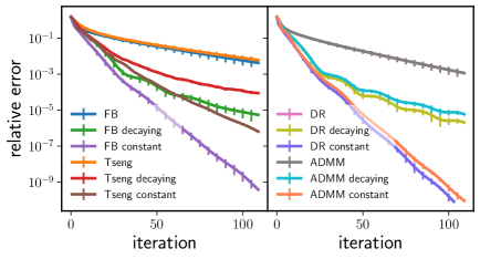
Figure 7: Performance of several methods on problem (9.5). We perform 10 Monte-Carlo runs and show the mean and standard deviation (error bars) of the error $|\varphi(x_{k})-\varphi^{\star}|/\varphi^{\star}$ versus the iteration $k$. The accelerated variants have faster convergence.

Next, we consider a matrix completion problem which is also of fundamental importance in machine learning. The goal is to reconstruct a low-rank matrix where we are only allowed to observe a few of its entries. Moreover, we assume these entries are constrained to specified range. More precisely, suppose that for a low-rank matrix $M\in\mathbb{R}^{n\times m}$ we observe entries $(i,j)$ that are collected in a set $\Omega$: let $\mathcal{P}_{\Omega}:\mathbb{R}^{n\times m}\to\mathbb{R}^{n\times m}$ be the projection onto the support of observed entries. The observable data matrix is thus $M_{\textnormal{obs}}=\mathcal{P}_{\Omega}(M)$, where $\mathcal{P}_{\Omega}(M)_{ij}=M_{ij}$ if $(i,j)\in\Omega$ and $\mathcal{P}_{\Omega}(M)_{ij}=0$ otherwise. The goal is to estimate the missing entries of $M$. This can be done [35] by solving the convex problem $\min_{X}\|X\|_{*}$ such that $\mathcal{P}_{\Omega}(X)=\mathcal{P}_{\Omega}(M)$—here $\|X\|_{*}$ denotes the nuclear norm. We consider a modification of this approach by imposing constraints $a\leq X_{ij}\leq b$ for given constants $a$ and $b$. Specifically,

$$\min_{X\in\mathbb{R}^{n\times m}}\underbrace{\alpha\|X\|_{*}}_{\varphi_{1}}+\underbrace{\mathcal{I}_{[a,b]}(X)}_{\varphi_{2}}+\underbrace{\dfrac{1}{2}\|\mathcal{P}_{\Omega}(X)-\mathcal{P}_{\Omega}(M)\|_{F}^{2}}_{\varphi_{3}}$$ (9.6)

where $\|\cdot\|_{F}$ denotes the Frobenius norm, $\mathcal{I}_{[a,b]}(X)=0$ if $a\leq X_{ij}\leq b$ and $\infty$ otherwise. A higher $\alpha>0$ induces lower rank solutions. This problem can be solved with Algorithms 1 and 2 with the proximal operator

$$\operatorname{prox}_{h\|\cdot\|_{*}}(X)=UD_{h}(\Sigma)V^{T},$$ (9.7)

where $X=U\Sigma V^{T}$ is the singular value decomposition of $X$ and $D_{h}(\Sigma)_{ii}=\max\{\Sigma_{ii}-h,0\}$ (see [35] for details). The proximal operator of $\varphi_{2}$ is just the projection

$$\operatorname{prox}_{h\mathcal{I}_{[a,b]}}(X)_{ij}=\max\{a,\min(X_{ij},b)\}.$$ (9.8)

Moreover, $\nabla\varphi_{3}(X)=\mathcal{P}_{\Omega}(X-M)$. In our methods we choose the following stopping criterion:

$$\|X_{k+1}-X_{k}\|_{F}\big{/}\|X_{k}\|_{F}\leq\epsilon$$ (9.9)

where $\epsilon$ is a small tolerance. To evaluate performance we report the relative error

$$\|X_{k}-M\|_{F}\big{/}\|M\|_{F}.$$ (9.10)

Following Ref. [35], we generate a low-rank matrix as $M=L_{1}L_{2}^{T}$ where $L_{1},L_{2}\in\mathbb{R}^{100\times 5}$ with entries sampled i.i.d. from $\mathcal{N}(3,1)$. Thus $M$ has rank $5$ (with probability one) and each entry is positive with high probability (each test instance was checked to have positive entries). We sample $sn^{2}$ entries of $M$ uniformly, with a sampling ratio $s=0.4$ (i.e. only $40\%$ of the matrix $M$ is observed). We choose

$$\begin{split}a&=\min\{(M_{\textnormal{obs}})_{ij}\}-\sigma/2,\\ b&=\max\{(M_{\textnormal{obs}})_{ij}\}+\sigma/2,\end{split}$$ (9.11)

where $\sigma$ is the standard deviation of all entries of $M_{\textnormal{obs}}$. In terms of algorithm’s parameters, we choose a step size $h=1$ for all methods, $r=3$ for decaying damping (2.22), and $\eta=0.1$ for constant damping (2.21)—the choice of step size is standard for this type of problem with proximal methods, while the choice of damping was obtained with a rough grid search and provided good results. In the stopping criterion (9.9) we choose $\epsilon=10^{-10}$. In Fig. 10 we report the mean and standard deviation (error bars) across 10 randomly generated instances of problem (9.6) with $\alpha=3.5$; all methods terminate successfully and recover a matrix with the correct rank (for this choice of $\alpha$) and a final relative error of $\approx 5\times 10^{-3}$. The number of iterations of each method to achieve the tolerance error are reported in Fig. 10a.

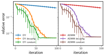
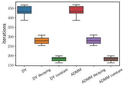
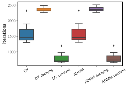
Figure 8: Convergence of different algorithms on problem (9.6). We perform $10$ Monte Carlo runs and indicate the mean and standard deviation (error bars) for the relative error (9.10) versus iteration $k$. Note the improvement of the accelerated methods.

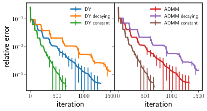
Figure 9: (a) Number of iterations needed to reach the termination tolerance for the problem in Fig. 10. (b) Number of iterations needed to reach the termination tolerance for the problem in Fig. 10.

Figure 10: Performance of different algorithms on problem (9.6) with annealing on $\alpha$.

To obtain more accurate solutions we consider “annealing” the parameter $\alpha$. We wish to verify if the accelerated methods can still speedup convergence in this scenario. We follow the procedure of [36] which is as follows. Given a sequence $\alpha_{1}>\alpha_{2}>\dotsm>\alpha_{L}=\bar{\alpha}>0$ for some $\bar{\alpha}$, we run each algorithm with $\alpha_{j}$ and then use its solution as a warm start for the solution to the next run with $\alpha_{j+1}$ (all other parameters are kept fixed). Starting with $\alpha_{0}=\delta\|M_{\textnormal{obs}}\|_{F}$ for some $\delta\in(0,1)$ we use the schedule

$$\alpha_{j+1}=\max\{\delta\alpha_{j},\bar{\alpha}\}$$ (9.12)

until reaching $\bar{\alpha}$. In our tests we choose $\delta=0.25$ and $\bar{\alpha}=10^{-8}$—these parameters were tuned with a few trials and proved to yield good results. The remaining parameters are the same as those used in creating Fig. 10, except that for the constant damping variants we now use $\eta=0.5$—in this example, overdamping the system yield better results. We report the convergence of different methods in Fig. 10. All methods successfully reach the termination tolerance, as for the previous test, but now achieve a better reconstruction accuracy. The total number of iterations in this case are shown in Fig. 10b. Note that, in this experiment, the decaying damping variants did not improve over the nonaccelerated method, but the constant damping variants still provided a significant improvement. This has to do with the “hardness” of the problem, i.e., due to the choice of rank and sampling ratio the objective function should have high curvature and this is why the overdamped case is faster (recall Fig. 1).

We now provide a real world example where the goal is to reconstruct a partially observed image. We pick a gray scale image, and by a singular value decomposition we truncate its first 70 eigenvalues. The end result is the image shown in Fig. 11a, represented by a $974\times 1194$ matrix with entries between $0$ and $1$ and of low rank $r=70$—this image will not be used as input data but will serve as the ground truth $M$. Then, we sample some of its entries uniformly with sampling ratio $s=0.3$, obtaining the image shown in Fig. 11b—this is the input data $M_{\textnormal{obs}}$ and has only $30\%$ of the original entries. This problem is actually hard, e.g., the number of effective degrees of freedom is $r(n+m-r)/(snm)\approx 0.42$ (see [35] for details).

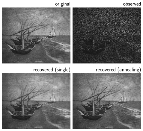
Figure 11: (a) Image of $974\times 1194$ pixels with rank $r=70$. (b) Observed data with sampling ratio $s=0.3$. (c) Reconstructed image by running the previous algorithms a single time. The relative error is $8\times 10^{-2}$—see Fig. 12 for convergence rates. (d) Reconstructed image with annealing. The relative error is $1.6\times 10^{-4}$—see Fig. 12 for convergence rates. The correct rank is also recovered by all methods.

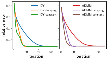
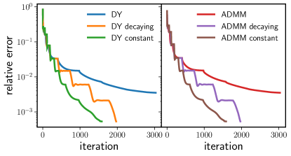
Figure 12: (a) Convergence rates of different methods when reconstructing the observed image in Fig. 11b by solving (9.6). An example of the recovered image is in Fig. 11c. (b) Convergence rates for the same problem but with annealing on $\alpha$. An example of the recovered image with the accelerated methods is shown in Fig. 11d—the nonaccelerated methods were unable to achieve such a small error.

By solving the nonnegative matrix completion problem (9.6)—with $a=0$ and $b=1$—our goal is to recover $M$ from $M_{\textnormal{obs}}$. As before, by running the previous algorithms a single time we recover the image shown in Fig. 11c. The convergence rates of different methods are shown in Fig. 12—in this case we choose $\alpha=1$, $\eta=0.1$ for constant damping (2.21), $r=3$ for decaying damping (2.22), step size $h=1$, and tolerance $\epsilon=10^{-6}$ in (9.9). Note how the accelerated variants achieve faster convergence. All methods recovered the correct rank.

To obtain more accurate results, we again consider annealing $\alpha$ according to (9.12)—we choose $\delta=0.25$ and $\bar{\alpha}=10^{-4}$, which was the smallest feasible value we found through several trials. An example of the recovered image—with the accelerated variants since the base methods were unable to achieve such a low error—is shown in Fig. 11d. By a closer inspection one can verify that Fig. 11d is actually better than Fig. 11c, e.g., has a better resolution. The convergence rates of each method under this setting are shown in Fig. 12. In this example, both accelerated variants—i.e., constant and decaying damping—were able to significantly improve over the base methods. Since this is a harder problem compared to the case of Fig. 10, the objective function should have less curvature thus underdamping the system yield better results.

10 Discussion and outlook

The main goal of this paper was to provide a unified perspective on standard optimization methods from a physics standpoint—these results are summarized in Fig. 4. We showed that there is indeed a unifying principle behind several well-known, but also new, optimization methods. The most general situation can be described by an underdamped Langevin equation, which accounts for accelerated methods in a stochastic setting. The randomness comes from a stochastic approximation to gradients or proximal operators—this has similarities to a Gaussian perturbation from a heat bath in a standard Langevin dynamics. When the minibatch is sufficiently large, i.e., the “temperature” $T\sim S^{-1}\to 0$, we recover the deterministic setting that is described by a dissipative form of Newton’s equation. In addition, in the high friction limit $\eta\to\infty$, the dynamics becomes nonaccelerated and thus described by an overdamped Langevin or by a first-order gradient flow, in the stochastic and deterministic regimes, respectively. All the optimization methods we discussed arise as discretizations of such systems. Thus, the fact that many seemingly unrelated optimization algorithms consist of actual simulations of the same dissipative physical system is quite surprising given that most of these methods were originally introduced from a completely independent approach, and without any connection to physics.

Using ODE splitting ideas and implicit discretizations, we introduced several accelerated and stochastic generalizations of the most important proximal algorithms in the literature. Moreover, important gradient-based methods, such as gradient descent, heavy ball, and Nesterov, also fit our framework; in these cases there is no splitting of the objective function and they correspond to explicit discretizations (see the Appendix). Interestingly, the heavy ball method turns out to be a structure-preserving (i.e., conformal symplectic) integrator, while Nesterov introduces a spurious dissipation; see Ref. [21] for details. Let us also point out that recently we generalized symplectic integrators to general dissipative Hamiltonian systems [33], which may offer a systematic approach to construct new gradient-based optimization methods based on simulations of physical systems.

The results of this paper explain why some different optimization methods may actually behave quite similarly in practice; the reason is because they are numerical integrators to the same physical system and have the same order of accuracy. Therefore, at this level, it is not possible to distinguish between different methods. However, the connections we established allow one to perform backward error analysis, which would result into modified ODEs that capture how a particular discretization perturbs the original system—we carried out such an analysis in the case of heavy ball and Nesterov [21]. It would thus be interesting to consider a similar analysis to some of the proximal methods previously discussed. This would bring refined insights and a better understanding of these methods. Another interesting question concerns the choice of damping. We considered constant (2.21) and decaying (2.22) damping since these cases are well-understood, e.g., we know some convergence rates and exact solutions in the quadratic case, as described in Sec. 3. However, other choices are possible and establishing the “optimal” damping strategy for a given problem class is an interesting and nontrivial problem.

It is worth mentioning that the connections between stochastic optimization and Langevin dynamics offers an interesting opportunity for bringing techniques from perturbation theory and nonequilibrium statistical mechanics into machine learning. For instance, any Fokker-Planck equation is equivalent to a path integral through the Martin-Siggia-Rose formalism [37]; this is a good starting point to apply field theory techniques to such problems. However, the optimization methods we considered may be applied to numerical problems in physics. For instance, there is a close connection between statistical mechanics and combinatorial optimization problems, such as finding ground states of spin glasses [38, 39]. The proximal methods considered in this paper can be adapted to tackle combinatorial problems such as max-cut and graph partitioning, which are somehow equivalent. Notably, in the context of machine learning and signal processing, proximal methods have been applied to large-scale problems with great success and proved to be quite efficient. It seems interesting to consider whether such an approach can lead to scalable and cheaper methods for disordered systems compared to standard Monte Carlo approaches.

Finally, it is thus clear that standard optimization methods are nothing but simulations of classical dissipative systems. A natural question concerns extending this perspective to the quantum level. Can we construct quantum optimization algorithms by simulating dissipative quantum systems? Open quantum systems is still a controversial topic, but they may offer an alternative to quantum annealing, whose discretizations may yield general quantum optimization algorithms. Thus, in the same way that a classical computer is employed to implement standard—i.e., classical—optimization algorithms, or equivalently to simulate a classical dissipative systems, perhaps a quantum computer may be necessary to simulate a dissipative quantum system [40].

Acknowledgments

GF thanks Michael I. Jordan for helpful discussions and Patrick Johnstone for comments on an earlier draft of this paper. We also thank the anonymous referees for insightful comments that helped to improve the paper. This work was supported by grants ARO MURI W911NF-17-1-0304, NSF 2031985, and NSF 1934931.

Appendix A Stochastic gradient descent, heavy ball,
and Nesterov

Since stochastic versions of gradient descent, heavy ball, and Nesterov’s method are widely used in machine learning, here we show how these methods arise from the previous physical systems.

Let us start with gradient descent. An explicit Euler-Maruyama discretization of the Langevin equation (8.12) yields

$$\begin{split}x_{k+1}&=x_{k}-h\nabla\varphi(x_{k})+\dfrac{h}{\sqrt{S}}C(x_{k})\epsilon_{k}\\ &=x_{k}-h\widetilde{\nabla\varphi}(x_{k}),\end{split}$$ (A.1)

where in the last passage we used (8.11) and (8.4). This is nothing but the well-known stochastic gradient descent (SGD) method, widely used in training neural networks. When $S\to\infty$, i.e. the stochastic gradient becomes the true gradient, $\widetilde{\nabla\varphi}\to\nabla\varphi$, we recover the deterministic gradient descent.

Let us now consider Nesterov’s method. Writing the underdamped Langevin (8.13) as

$$\ddot{x}=-\nabla\varphi(x)-\eta(t)\dot{x}+\sqrt{\dfrac{h}{S}}C(x)\dot{W},$$ (A.2)

where this should be understood in the Itô sense, we discretize it with the help of (2.18), (8.11) and (8.4) to obtain

$$\begin{split}\dfrac{x_{k+1}-\hat{x}_{k}}{h^{2}}&=-\nabla\varphi(\hat{x}_{k})+\dfrac{1}{\sqrt{S}}C(\hat{x}_{k})\epsilon_{k}\\ &=-\widetilde{\nabla\varphi}(\hat{x_{k}}).\end{split}$$ (A.3)

Recalling the definition (2.17), and redefining the step size as usual, $h^{2}\mapsto h$, we obtain

$$x_{k+1} =\hat{x}_{k}-h\widetilde{\nabla\varphi}(\hat{x}_{k}),$$ (A.4a)

$$\hat{x}_{k+1} =x_{k+1}+\gamma_{k+1}(x_{k+1}-x_{k}).$$ (A.4b)

This is a stochastic version of Nesterov’s method—the original method is recovered in the deterministic case where $S\to\infty$.

Let us now consider Polyak’s heavy ball method. From a physics point of view this case is more interesting since the deterministic method was recently shown by us [33] to be a conformal symplectic integrator. Consider the underdamped Langevin equation (8.13). We write the second equation as

$$\dfrac{d}{dt}\left(e^{\theta(t)}p\right)=-e^{\theta(t)}\nabla\varphi(x)+e^{\theta(t)}\sqrt{\dfrac{h}{S}}C(x)\dot{W},$$ (A.5)

where $\dot{\theta}(t)\equiv\eta(t)$. Integrating this from $t_{k}$ to $t_{k+1}=t_{k}+h$, and keeping terms up to $\mathcal{O}(h^{2})$, we get

$$\begin{split}p_{k+1}&=e^{-h\eta_{k}}p_{k}-h\nabla\varphi(x_{k})+\dfrac{h}{\sqrt{S}}C(x_{k})\epsilon_{k}\\ &=e^{-h\eta_{k}}p_{k}-h\widetilde{\nabla\varphi}(x_{k}).\end{split}$$ (A.6)

The first equation in (8.13) gives

$$x_{k+1}=x_{k}+hp_{k+1}+\mathcal{O}(h^{2}).$$ (A.7)

Now we define the following variables:

$$\mu_{k}\equiv e^{-h\eta_{k}},\qquad v_{k}\equiv hp_{k},\qquad h^{2}\mapsto h.$$ (A.8)

This allows us to write (A.6) and (A.7) as

$$v_{k+1} =\mu_{k}v_{k}-h\widetilde{\nabla\varphi}(x_{k}),$$ (A.9a)

$$x_{k+1} =x_{k}+v_{k+1}.$$ (A.9b)

This is precisely a stochastic version of the heavy ball method, often referred to as momentum method, or SGD with momentum, in deep learning literature. Usually this method is used with a constant $\eta_{k}=\eta$, in which case $\mu\equiv e^{-h\eta}\in(0,1]$ is known as the “momentum factor.” When $S\to\infty$, i.e. the stochastic gradient becomes the true gradient, the above recovers the deterministic heavy ball method. Therefore, once again, the scheme of Fig. 4 also apply to gradient-based methods. Compared to the proximal methods previously discussed, the difference in these cases is that the gradient is always computed explicitly as opposed to implicitly.

References

- [1] A. Cauchy, “Méthode générale pour la résolution des systèmes d’équations simultanées,” C. R. Acad. Sci. Paris 25 (1847) 536–538.
- [2] J. Douglas and H. H. Rachford, “On the numerical solution of heat conduction problems in two and three space variables,” Trans. Amer. Math. Soc. 82 (1956) 421–439.
- [3] R. Glowinski and A. Marroco, “Sur l’approximation, par él’ements finis d’ordre un, et la résolution, par pénalisation-dualité d’une classe de probèmes de Dirichlet non linéaires,” ESAIM: Mathematical Modelling and Numerical Analysis - Modélisation Mathématique et Analyse Numérique 9 no. R2, (1975) 41–76.
- [4] D. Gabay and B. Mercier, “A dual algorithm for the solution of nonlinear variational problems via finite element approximations,” Computers and Mathematics with Applications 2 no. 1, (1976) 17–40.
- [5] S. Boyd, N. Parikh, E. Chu, B. Peleato, and J. Eckstein, “Distributed optimization and statistical learning via the alternating direction method of multipliers,” Foundations and Trends in Machine Learning 3 no. 1, (2011) 1–122.
- [6] P. L. Lions and B. Mercier, “Splitting algorithms for the sum of two nonlinear operators,” SIAM J. Numer. Anal. 16 no. 6, (1979) 964–979.
- [7] P. Tseng, “A modified forward-backward splitting method for maximal monotone mappings,” SIAM J. Control Optim. 38 no. 2, (2000) 431–446.
- [8] D. Davis and W. Yin, “A three-operator splitting scheme and its optimization applications,” Set-Valued and Variational Analysis 25 (2017) 829–858.
- [9] E. K. Ryu and S. Boyd, “A primer on monotone operator methods,” Appl. Comput. Math. 15 no. 1, (2016) 3–43.
- [10] N. Parikh and S. Boyd, “Proximal algorithms,” Foundations and Trends in Optimization 1 no. 3, (2013) 123–231.
- [11] F. E. Browder, “Nonlinear elliptic boundary value problems,” Bull. Amer. Math. Soc. 69 no. 6, (1963) 862–874.
- [12] F. E. Browder, “The solvability of non-linear functional equations,” Duke Math J. 30 no. 4, (1963) 557–566.
- [13] F. E. Browder, “Variational boundary value problems for quasi-linear elliptic equations of arbitrary order,” Proc. Nat. Acad. Sci. 50 no. 1, (1963) 31–37.
- [14] G. J. Minty, “Monotone (nonlinear) operators in Hilbert space,” Duke Math. J. 29 no. 3, (1962) 341–346.
- [15] H. H. Bauschke and P. L. Combettes, Convex Analysis and Monotone Operator Theory in Hilbert Spaces. Springer International Publishing, 2017.
- [16] E. Zeidler, Nonlinear Functional Analysis and its Applications, II/B: Nonlinear Monotone Operators. Springer-Verlag, 1990.
- [17] B. T. Polyak, “Some methods of speeding up the convergence of iteration methods,” USSR Comp. Math. and Math. Phys. 4 no. 5, (1964) 1–17.
- [18] Y. Nesterov, “A method of solving a convex programming problem with convergence rate ,” Soviet Mathematics Doklady 27 no. 2, (1983) 372–376.
- [19] W. Su, S. Boyd, and E. J. Candès, “A differential equation for modeling Nesterov’s accelerated gradient method: Theory and insights,” J. Mach. Learn. Res. 17 no. 153, (2016) 1–43.
- [20] A. Wibisono, A. C. Wilson, and M. I. Jordan, “A variational perspective on accelerated methods in optimization,” Proc. Nat. Acad. Sci. 113 no. 47, (2016) E7351–E7358.
- [21] G. França, J. Sulam, D. P. Robinson, and R. Vidal, “Conformal symplectic and relativistic optimization,” J. Stat. Mech. 2020 no. 12, (2020) 124008, arXiv:1903.04100 [math.OC].
- [22] P. Caldirola, “Forze non conservative nella meccanica quantistica,” Nuovo Cim. 18 (1941) 393–400.
- [23] E. Kanai, “On the quantization of the dissipative systems,” Prog. Theor. Phys. 3 (1948) 440–442.
- [24] A. O. Caldeira and A. J. Leggett, “Influence of dissipation on quantum tunneling in macroscopic systems,” Phys. Rev. Lett. 46 no. 4, (1981) 211–214.
- [25] R. I. McLachlan and G. R. W. Quispel, “Splitting methods,” Acta Numerica 11 (2002) 341–434.
- [26] R. L. Speth, W. H. Green, S. MacNamara, and G. Strang, “Balanced splitting and rebalanced splitting,” SIAM J. Numer. Anal. 51 no. 6, (2013) 3084–3105.
- [27] G. França, D. P. Robinson, and R. Vidal, “ADMM and accelerated ADMM as continuous dynamical systems,” Int. Conf. Machine Learning (2018) , arXiv:arXiv:1805.06579 [math.OC].
- [28] G. França, D. P. Robinson, and R. Vidal, “A nonsmooth dynamical systems perspective on accelerated extensions of ADMM,” arXiv:arXiv:1808.04048 [math.OC].
- [29] E. Hairer, C. Lubich, and G. Wanner, Geometric Numerical Integration. Springer, 2006.
- [30] T. Goldstein, B. O’Donoghue, S. Setzer, and R. Baraniuk, “Fast alternating direction optimization methods,” SIAM J. Imag. Sci. 7 no. 3, (2014) 1588–1623.
- [31] P. Patrinos, L. Stella, and A. Bemporad, “Douglas-Rachford splitting: complexity estimates and accelerated variants,” in 53rd IEEE Conf. Dec. and Control, pp. 4234–4239. 2014.
- [32] A. Beck and M. Teboulle, “A fast iterative shrinkage-thresholding algorithm for linear inverse problems,” SIAM J. Imag. Sci. 2 no. 1, (2009) 183–202.
- [33] G. França, M. I. Jordan, and R. Vidal, “On dissipative symplectic integration with applications to gradient-based optimization,” J. Stat. Mech. 2021 no. 4, (2021) 043402, arXiv:2004.06840 [math.OC].
- [34] H. Robbins and S. Monro, “A stochastic approximation method,” Ann. Math. Statist. 22 no. 3, (1951) 400–407.
- [35] J. Cai, E. Candès, and Z. Shen, “A singular value thresholding algorithm for matrix completion,” SIAM Journal on Optimization 20 no. 4, (2010) 1956–1982.
- [36] S. Ma, D. Goldfarb, and L. Chen, “Fixed point and Bregman iterative methods for matrix rank minimization,” Math. Prog. 128 (2011) 321–353.
- [37] J. Zinn-Justin, Quantum Field Theory and Critical Phenomena. Clarendon Press, 2002.
- [38] M. Mezard, G. Parisi, and M. A. Virasoro, Spin Glass Theory and Beyond. World Scientific, 1987.
- [39] H. Nishimori, Statistical Physics of Spin Glasses and Information Processing: An Introduction. Clarendon Press, 2001.
- [40] R. P. Feynman, “Simulating physics with computers,” Int. J. Theor. Phys. 21 (1982) 467–488.