Voter model on networks partitioned into two cliques of arbitrary sizes

Abstract

The voter model is an archetypal stochastic process that represents opinion dynamics. In each update, one agent is chosen uniformly at random. The selected agent then copies the current opinion of a randomly selected neighbour. We investigate the voter model on a network with an exogenous community structure: two cliques (i.e. complete subgraphs) randomly linked by $X$ interclique edges. We show that, counterintuitively, the mean consensus time is typically not a monotonically decreasing function of $X$. Cliques of fixed proportions with opposite initial opinions reach a consensus, on average, most quickly if $X$ scales as $N^{3/2}$, where $N$ is the number of agents in the network. Hence, to accelerate a consensus between cliques, agents should connect to more members in the other clique as $N$ increases but not to the extent that cliques lose their identity as distinct communities. We support our numerical results with an equation-based analysis. By interpolating between two asymptotic heterogeneous mean-field approximations, we obtain an equation for the mean consensus time that is in excellent agreement with simulations for all values of $X$.

Keywords: voter model, community structure, consensus time, heterogeneous mean-field approximation, complex networks

1 Introduction

Opinion formation in social networks has become an active field of research in statistical physics (for reviews, see [1, 2, 3]). In particular, the voter model [4, 5] has become a paradigmatic model for opinion dynamics. Its rules are simple but sufficiently powerful to reproduce the summary statistics of real elections [6]. In the basic version of the voter model, the vertices on a network represent agents that can hold exactly one of two possible opinions: ‘red’ or ‘blue’. Repeatedly, one agent is selected independently and uniformly at random. This agent then adopts the opinion of a randomly chosen adjacent agent (figure 1). As long as the network is connected and finite, this update rule guarantees that agents must eventually reach a consensus [7], defined as a state in which all agents have identical opinions.

Figure 1: Illustrative example of a small two-clique network. In this example, clique 1 is a complete subgraph with seven vertices (circles), whereas clique 2 has only five vertices (squares). Each vertex represents an agent that has exactly one of two possible opinions: ‘red’ or ‘blue’. We apply the update rules of the voter model. That is, we first choose a random focal vertex, e.g. $A$, in the depicted network. Then, we choose a random neighbour of the focal vertex and copy the neighbour’s opinion. In our example, if the chosen neighbour is $B$, $A$ changes its opinion to blue. If the chosen neighbour is $C$, $A$ keeps its current (i.e. red) opinion. We distinguish between intraclique edges (thin lines) and interclique edges (thick lines). In our analysis, we vary the relative sizes of the two cliques and the number of interclique edges.

The mean time until consensus depends on the initial distribution of opinions and the network structure. While early studies of the voter model focused on complete graphs [8] or regular lattices [9], interest has recently shifted towards networks with more complex topologies, e.g. small-world networks [10, 11], graphs with right-skewed degree distributions [12, 13, 14, 15], multiplex networks [16], or networks with a community structure [17, 18, 19].

A subgraph of a network is called a community if there are significantly more edges within the subgraph and fewer links to the rest of the network than those predicted by a null model that has no planted community structure (e.g. an Erdős–Rényi graph with the same total number of edges as the network under investigation) [20]. The detection of communities from network data has become a major line of research with a plethora of different algorithmic approaches [21]. Various techniques have confirmed that essentially all networks of practical relevance contain more than a single community [22, 23, 24, 25, 26].

This finding has motivated us to analyse the voter model for one of the simplest possible types of multi-community networks—namely, networks with exactly two communities. Situations where agents divide into two communities are plentiful in the real world. For example, a split between communities may arise because of a language barrier (e.g. between Dutch and French speakers in Belgium [27]) or differences in race, ethnicity, age, religion, education, occupation, or gender [28]. Conversely, agents with similar attributes tend to form close-knit communities because of status homophily [29], a social phenomenon that causes the proverbial birds of a feather to flock together. Within communities, cohesion often reaches such an extent that ‘we can observe in many groups a social unity within which people feel at one though their opinions still differ’ (p. 229 in [30]).

Previously, it has been claimed that the voter model is insensitive to changes in the community structure [31]. This conclusion has mainly rested on results for two equally large cliques (i.e. complete subgraphs), where the mean consensus time is proportional to the total number of vertices in the network, $N$, unless the connections between cliques are extremely sparse [32, 18]. Here, we argue that an investigation of only the special case of equally large cliques does not do justice to the actual complexity of the problem.

In this article, we revisit the two-clique voter model but allow unequal clique sizes. The dynamics exhibit an intriguing feature: the mean consensus time is minimal at an intermediate interclique connectivity. We investigate in detail the case where cliques with given relative sizes start from opposite opinions, representing a completely polarised society. To minimise the mean consensus time, we find that the optimal number of interclique edges, $X_{\rm min}$, should scale in proportion to $N^{3/2}$. This scaling law puts $X_{\rm min}$ between the case of a constant number of interclique links per agent ($X\propto N$) and a complete graph ($X\propto N^{2}$).

After specifying the details of our model in section 2, we present the results from numerical simulations in section 3. In section 4, we derive an analytical expression for the mean consensus time as a function of $X$ for arbitrary clique sizes. Our derivation demonstrates how we can go beyond previous approximations [18, 33] to obtain not only the asymptotic behaviour for either extremely sparsely or densely connected cliques, but also reliable predictions for the intermediate interclique connectivity. We conclude with a discussion of our results in section 5.

2 Model

We consider a simple undirected graph with $N$ vertices that can be partitioned into two cliques, as shown in figure 1. We denote the fraction of vertices in the first clique by $\alpha\in(0,1)$. The two cliques are connected by $X$ edges randomly selected from all $\alpha(1-\alpha)N^{2}$ possible pairs that can be formed by one vertex in clique $1$ and another vertex in clique $2$.

Each vertex is either red or blue depending on the current opinion of the corresponding agent. The time intervals between consecutive opinion updates are independent, identically distributed exponential random numbers so that the dynamics are a continuous-time Markov chain. We choose the time unit such that every individual agent is active with a rate equal to $1$.

If we wish to keep track of all individual opinions, the cardinality of the model’s state space is $2^{N}$. The Monte Carlo algorithm behind all numerical data presented in this paper is in fact based on this exact agent-based paradigm. However, summarising and modelling the results at such a fine level of resolution is neither insightful nor practical given that the number of configurations grows exponentially with $N$. Instead, we combine all configurations whose fraction of red agents is $\rho_{1}$ in clique $1$ and $\rho_{2}$ in clique $2$ into the macrostate $(\rho_{1},\rho_{2})$ to simplify the data analysis, visualisation, and mathematical modelling. Strictly speaking, the Markov chain is not lumpable at this macroscopic level [34] because we neglect the fact that different vertices in a clique can be adjacent to a different number of vertices in the other clique. Let us denote the number of interclique edges incident on a vertex $v$ by $k_{{\rm inter},v}$. The probability distribution of $k_{{\rm inter},v}$ is approximately binomial; thus, it is so concentrated near its peak that we withhold little information if we replace the exact value $k_{{\rm inter},v}$ with its mean: $k_{{\rm inter},v}\approx X/(\alpha N)$ for all vertices $v$ in clique $1$ and $k_{{\rm inter},v}\approx X/[(1-\alpha)N]$ for every $v$ in clique $2$. In the parlance of statistical physics, we apply a heterogeneous mean-field approximation [7, 35]: we correctly account for the difference in the clique sizes and replace the exact microscopic interactions with an average over the cliques. More elaborate approximations are conceivable [18], but the mean-field approximation is remarkably accurate, as we will see shortly. On balance, we do not find the notational burden of a more detailed approximation to be worth the effort.

Table 1: Transitions from the state $(\rho_{1},\rho_{2})$ and their rates.

New state	How is the new	Transition rate matrix element
$(y,z)$	state reached?	$Q[(\rho_{1},\rho_{2}),(y,z)]$
$\left(\rho_{1}+\frac{1}{\alpha N},\rho_{2}\right)$	A blue agent in clique $1$ adopts	$\alpha N(1-\rho_{1})\cdot\frac{\alpha N(\alpha N-1)\rho_{1}\,+\,X\rho_{2}}{\alpha N(\alpha N-1)\,+\,X}$
	the opinion of a red agent.
$\left(\rho_{1}-\frac{1}{\alpha N},\rho_{2}\right)$	A red agent in clique $1$ adopts	$\alpha N\rho_{1}\cdot\frac{\alpha N(\alpha N-1)(1-\rho_{1})\,+\,X(1-\rho_{2})}{\alpha N(\alpha N-1)\,+\,X}$
	the opinion of a blue agent.
$\left(\rho_{1},\rho_{2}+\frac{1}{(1-\alpha)N}\right)$	A blue agent in clique $2$ adopts	$(1-\alpha)N(1-\rho_{2})\,\cdot$
	the opinion of a red agent.	$\frac{(1-\alpha)N[(1-\alpha)N-1]\rho_{2}\,+\,X\rho_{1}}{(1-\alpha)N[(1-\alpha)N-1]\,+\,X}$
$\left(\rho_{1},\rho_{2}-\frac{1}{(1-\alpha)N}\right)$	A red agent in clique 2 adopts	$(1-\alpha)N\rho_{2}\,\cdot$
	the opinion of a blue agent.	$\frac{(1-\alpha)N[(1-\alpha)N-1](1-\rho_{2})\,+\,X(1-\rho_{1})}{(1-\alpha)N[(1-\alpha)N-1]\,+\,X}$
$(\rho_{1},\rho_{2})$	Negative sum of all rates above.

Applying these simplifications, we can derive the transition rate matrix $\mathbf{Q}$. For example, if a blue agent in clique $1$ becomes red, the state changes from $(\rho_{1},\rho_{2})$ to $\left(\rho_{1}+\frac{1}{\alpha N},\rho_{2}\right)$. This transition occurs with a rate that is the product of the following two factors. The first factor is the number of blue agents in clique $1$, which is equal to $\alpha N(1-\rho_{1})$. The second factor is the fraction of adjacent agents whose opinion is red. Because an agent in clique $1$ is connected to $\alpha N-1$ agents in clique $1$ and, on average, to $X/(\alpha N)$ agents in clique $2$, we obtain the transition rate

$$Q\left[(\rho_{1},\rho_{2}),\left(\rho_{1}+\frac{1}{\alpha N},\rho_{2}\right)\right]=\alpha N(1-\rho_{1})\cdot\frac{(\alpha N-1)\rho_{1}+\frac{X}{\alpha N}\,\rho_{2}}{\alpha N-1+\frac{X}{\alpha N}}\ .$$

With similar arguments, we can also deduce the remaining elements of $\mathbf{Q}$. In table 1, we list all nonzero transition rates. As is convention, we set the diagonal terms of $\mathbf{Q}$ equal to the negative sum of all other terms in that row [36]: $Q(\boldsymbol{\rho},\boldsymbol{\rho})=-\sum_{\boldsymbol{\rho}^{\prime}\neq\boldsymbol{\rho}}Q(\boldsymbol{\rho},\boldsymbol{\rho}^{\prime})$, where $\boldsymbol{\rho}=(\rho_{1},\rho_{2})$. For our simulations, we apply the exact agent-based update rules of the voter model and take the exact network topology into account where the degrees are not the same for all vertices in a clique. For the analytical solution in section 4, however, we resort to the approximations that are implicit in $\mathbf{Q}$.

3 Simulation results

To build intuition about the model, we show how the dynamics unfold during several sample runs with $N=500$ and $\alpha=0.8$ in figure 2. We start the cliques in a state of complete polarisation: within each clique, opinions are initially unanimous, but there is disagreement between cliques so that either $(\rho_{1},\rho_{2})=(1,0)$ or $(\rho_{1},\rho_{2})=(0,1)$.

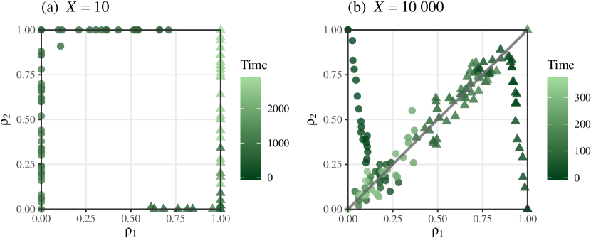
Figure 2: Example trajectories for a two-clique graph with $N=500$ vertices and $\alpha=0.8$ (i.e. $400$ vertices are in the first clique, $100$ in the second). Triangles and circles represent different sample runs of the dynamics. To avoid overplotting, we only show approximately 50 points during each run. (a) With only $X=10$ interclique edges, the states remain close to the boundaries of the plot (i.e. at least one of the cliques is internally almost unanimous). (b) If $X=10\,000$, the system rapidly moves from a state of complete polarisation (top-left or bottom-right corner) towards the diagonal line ($\rho_{1}=\rho_{2}$). The trajectory then remains near the diagonal line until it reaches one of the two consensus states in the top-right or bottom-left corner of the plot.

In figure 2(a), there are only $X=10$ interclique edges; thus, it is difficult for an opinion to invade the clique that started from the opposite opinion. Fluctuations occur in only one clique at a time. Meanwhile, the other clique remains almost unwavering in its support of its starting opinion. As a consequence, the trajectory shown in figure 2(a) mostly remains around the edges of the two-dimensional state space $(\rho_{1},\rho_{2})\in[0,1]^{2}$. After a protracted tug of war, confidence in the starting opinion ultimately vanishes in one of the cliques—usually the smaller one, with a probability that we will quantify in equation (7) below—so that the system reaches one of the two absorbing states $(0,0)$ or $(1,1)$.

By contrast, if $X=10\,000$, the proportions of red agents $\rho_{1}$ and $\rho_{2}$ rapidly approach equality, as shown in figure 2(b). Afterwards, the dynamics in one clique almost instantaneously follow the trends in the other clique so that the trajectory is confined to the vicinity of the diagonal line $\rho_{1}=\rho_{2}$. In this case, the cliques behave as one integrated entity despite being only loosely connected by the network topology.

The distinct behaviours of the model for small and large $X$ lead to substantially different consensus times, which are evident when comparing the limits of the colour bar legends in figures 2(a) and 2(b). For $X=\Or(1)$, it can take an extremely long time to reach a consensus because the cliques hardly exchange any opinions. If $X\gg 1$, the cliques communicate more frequently with each other and therefore typically agree on a final opinion sooner. However, the mean consensus time does not necessarily monotonically decrease with $X$, as we will now see.

Figure 3: Dependence of the mean consensus time $\langle T_{\rm pol}\rangle$ on the number of interclique edges $X$. Each point represents numerical data from 2000 Monte Carlo simulations with a polarised initial condition (i.e. cliques are internally unanimous, but the cliques disagree with each other). Error bars represent 95% confidence intervals. All curves illustrate predictions from the equation-based method described in section 4. We emphasise that there are no free parameters in the equations; hence, none of the curves shown here needed to be fitted to data. (a) We fix $N=1000$ and vary $\alpha$. (b) We hold $\alpha=0.9$ constant, but $N$ varies. (c) The same data as in (a) and (b) but with rescaled coordinate axes. We plot $\xi=X/N$ along the horizontal axis and $\tau=\left(\frac{1}{\alpha^{2}}+\frac{1}{(1-\alpha)^{2}}\right)\langle T_{\rm pol}\rangle/N$ along the vertical axis. The dashed line represents the reciprocal relationship $\tau=1/\xi$. (d) The number of edges $X_{\rm min}$ that minimises $\langle T_{\rm pol}\rangle$ follows the power law $X_{\rm min}\propto N^{3/2}$ predicted by equation (22).

We denote the consensus time from the completely polarised initial state $(\rho_{1},\rho_{2})=(1,0)$ by $T_{\rm pol}$ and its mean by $\langle T_{\rm pol}\rangle$, which is an average over different realisations of the stochastic voter-model dynamics and over different randomly sampled networks with $X$ interclique edges. In figure 3(a), we show simulation results for $\langle T_{\rm pol}\rangle$ as a function of $X$ for $N=1000$ and different values of $\alpha$. Because the dynamics for $\alpha$ and $1-\alpha$ are identical if we exchange the labels of the cliques and opinions, we only plot results for $\alpha\geq\frac{1}{2}$. For all values of $\alpha$, $\langle T_{\rm pol}\rangle$ attains its maximum at $X=1$ and initially decreases as we insert more interclique edges, consistent with the intuition that more connections lead to a faster consensus. Surprisingly, however, if $\alpha\neq\frac{1}{2}$, the trend reverses as we keep increasing $X$: $\langle T_{\rm pol}\rangle$ passes through a minimum and then increases again as the network becomes a complete graph, where $X=\alpha(1-\alpha)N^{2}$. This increase is more pronounced when the difference in clique sizes is larger. For $\alpha=0.9$, we can reduce the mean consensus time by $\approx 76\%$ if we cut $\approx 98\%$ of the interclique ties in the complete graph.

In figure 3(b), we fix $\alpha=0.9$ and vary $N$. In general, an increase in $N$ shifts the curves towards larger values of $\langle T_{\rm pol}\rangle$ and $X$. However, the curves’ overall shapes remain similar. The common pattern behind the data plotted in figures 3(a) and 3(b) becomes clearer in figure 3(c), where we plot the rescaled variable $\tau=\left(\frac{1}{\alpha^{2}}+\frac{1}{(1-\alpha)^{2}}\right)\langle T_{\rm pol}\rangle/N$ versus $\xi=X/N$. For $\xi\ll 1$, the rescaled functions collapse onto the same function $\tau=1/\xi$. The scaling relation $\tau\propto 1/\xi$ was pointed out for the special case $\alpha=\frac{1}{2}$ in [18]. Our simulations and the equation-based analysis in section 4 show that $\tau$ and $1/\xi$ are not merely proportional but equal in the limit $\xi\to 0$. This result is valid for all clique sizes assuming a completely polarised initial state. For other initial conditions, we also find that $\tau\propto 1/\xi$ but with different proportionality factors, which can be calculated with the method presented in section 4.

Figure 3(d) reveals another emergent scaling relation. In this scatterplot, the abscissa is the network size $N$. The ordinate is the number of interclique edges $X_{\rm min}$ that minimises $\langle T_{\rm pol}\rangle$. For each combination of $N$ and $\alpha$ in figure 3(d), we perform 2000 Monte Carlo simulations. We then estimate $X_{\rm min}$ from the locally estimated scatterplot smoothing (LOESS) regression curves and establish error bars with bootstrapping. For a fixed value of $\alpha$, the data follow the power law $X_{\rm min}\propto N^{3/2}$. Thus, to minimise the mean consensus time, the agents must strike a balance between a sparse and a dense interclique connectivity. On one hand, the optimal number of interclique links per agent grows as $k_{{\rm inter},v}\propto\sqrt{N}$. On the other hand, the optimal number of interclique edges $X_{\rm min}$ is only a vanishing fraction of the number $\alpha(1-\alpha)N^{2}$ of all possible interclique edges in the limit $N\to\infty$.

In summary, the Monte Carlo simulations reveal three main features of the two-clique voter dynamics starting from cliques with opposite opinions. First, $\langle T_{\rm pol}\rangle$ is a U-shaped function of $X$ as long as $\alpha\neq\frac{1}{2}$. Notably, the global minimum does not coincide with a complete graph. Second, the mean consensus time obeys the identity $\tau=1/\xi$ or, equivalently,

$$\langle T_{\rm pol}\rangle=\frac{\alpha^{2}(1-\alpha)^{2}}{2\alpha^{2}-2\alpha+1}\frac{N^{2}}{X}$$ (1)

as long as $X\ll N$. Third, the number of interclique edges that minimises $\langle T_{\rm pol}\rangle$ satisfies the scaling relation $X_{\rm min}\propto N^{3/2}$. We now demonstrate how these results can be derived from the transition rates in table 1.

4 Equation-based analysis

Let us denote the mean consensus time conditioned on the initial opinions $(\rho_{1},\rho_{2})$ by $\langle T(\rho_{1},\rho_{2})\rangle$. With this notation, $\langle T_{\rm pol}\rangle=\langle T(1,0)\rangle$. Because $\langle T(\rho_{1},\rho_{2})\rangle$ is the mean exit time of a Markov chain with absorbing states $(0,0)$ and $(1,1)$, it must satisfy $\langle T(0,0)\rangle=\langle T(1,1)\rangle=0$ and [36]

$$\sum_{y,z}Q[(\rho_{1},\rho_{2}),(y,z)]\langle T(y,z)\rangle=-1$$

if $(\rho_{1},\rho_{2})\not\in\{(0,0),(1,1)\}$. Next, we insert $\mathbf{Q}$ from table 1 and perform, in the parlance of mathematical population genetics, a diffusion approximation [37]: we assume $N\gg 1$ and take the continuum limit. The result is the partial differential equation

$$\eqalign{\frac{(\alpha N-1)\rho_{1}(1-\rho_{1})+\frac{X}{2\alpha N}(\rho_{1}+\rho_{2}-2\rho_{1}\rho_{2})}{\alpha N(\alpha N-1)+X}\frac{\partial^{2}\langle T\rangle}{\partial\rho_{1}^{2}}\\ \quad+\frac{[(1-\alpha)N-1]\rho_{2}(1-\rho_{2})+\frac{X}{2(1-\alpha)N}(\rho_{1}+\rho_{2}-2\rho_{1}\rho_{2})}{(1-\alpha)N[(1-\alpha)N-1]+X}\frac{\partial^{2}\langle T\rangle}{\partial\rho_{2}^{2}}\\ \quad+\frac{X}{\alpha N(\alpha N-1)+X}(\rho_{2}-\rho_{1})\frac{\partial\langle T\rangle}{\partial\rho_{1}}\\ \quad+\frac{X}{(1-\alpha)N[(1-\alpha)N-1]+X}(\rho_{1}-\rho_{2})\frac{\partial\langle T\rangle}{\partial\rho_{2}}+O(N^{-2})\\ =-1.}$$ (2)

Finding an exact solution to equation (2) would be a formidable task, but the result would not be directly useful. Instead, we aim for an approximate solution. First, we find a solution that is valid if $X=\Or(N)$. Afterwards, we derive an approximation for the case where $X\gg N$. Finally, we interpolate between these two approximations to arrive at a solution that fits the data remarkably well over the entire range from $X=1$ to the complete graph with $X=\alpha(1-\alpha)N^{2}$. The solid curves in figure 3 are based on this interpolation.

4.1 Approximate solution if $X=\Or(N)$

For a sparse interclique connectivity, the leading terms of equation (2) up to and including $\Or\left(N^{-1}\right)$ are

$$\eqalign{&\frac{1}{\alpha N}\,\rho_{1}(1-\rho_{1})\frac{\partial^{2}\langle T\rangle}{\partial\rho_{1}^{2}}+\frac{1}{(1-\alpha)N}\rho_{2}(1-\rho_{2})\frac{\partial^{2}\langle T\rangle}{\partial\rho_{2}^{2}}\\ &\quad+\frac{X}{\alpha^{2}N^{2}}\,(\rho_{2}-\rho_{1})\frac{\partial\langle T\rangle}{\partial\rho_{1}}+\frac{X}{(1-\alpha)^{2}N^{2}}(\rho_{1}-\rho_{2})\frac{\partial\langle T\rangle}{\partial\rho_{2}}=-1.}$$ (3)

We are not aware of an exact solution to equation (3), but we assume that it can be expressed as a power series. The main features already become apparent when only expanding up to the quadratic terms. We denote this approximation by $t_{\rm sparse}$ to indicate that this expression is valid if we only have a sparse connectivity between cliques:

$$t_{\rm sparse}(\rho_{1},\rho_{2})=\sum_{i=0}^{2}\sum_{j=0}^{2}c_{i,j}\left(\rho_{1}-\frac{1}{2}\right)^{i}\left(\rho_{2}-\frac{1}{2}\right)^{j}\ .$$ (4)

Because $\langle T\rangle$ is symmetric with respect to $\left(\frac{1}{2},\frac{1}{2}\right)$, we must have $c_{i,j}=0$ if either $i$ is odd and $j$ is even or vice versa. Only five coefficients remain that can possibly be nonzero: $c_{0,0}$, $c_{0,2}$, $c_{1,1}$, $c_{2,0}$, and $c_{2,2}$. We can determine these coefficients from equation (3) and the boundary conditions. We skip the details here and instead refer to the appendix, where we show that

$$\eqalign{\langle T_{\rm pol}\rangle&\approx t_{\rm sparse}(1,0)=-\frac{1}{2}c_{1,1}\\ &=\frac{\alpha^{2}(1-\alpha)^{2}N}{Xd(\alpha,N,X)}\big{[}2(2\alpha^{2}-2\alpha+1)X^{3}+2(\alpha^{2}-\alpha+1)NX^{2}\\ &\hskip 85.35826pt+\alpha(1-\alpha)(2\alpha^{2}-2\alpha+3)N^{2}X+\alpha^{2}(1-\alpha)^{2}N^{3}\big{]}}$$ (5)

with the auxiliary function

$$\eqalign{d(\alpha,N,X)=&(3\alpha^{2}-3\alpha+1)(2\alpha^{2}-2\alpha+1)X^{2}\\ &+\alpha(1-\alpha)(4\alpha^{4}-8\alpha^{3}+11\alpha^{2}-7\alpha+2)NX\\ &+\alpha^{2}(1-\alpha)^{2}(2\alpha^{2}-2\alpha+1)N^{2}}$$ (6)

in the denominator.

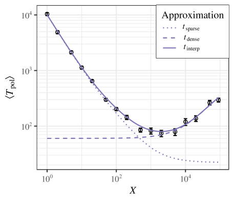
Figure 4: Illustration of the approximations for $\langle T_{\rm pol}\rangle$ presented in section 4. As an example, we show data for $N=1000$ and $\alpha=0.9$ as open circles. Each circle represents the mean of 2000 Monte Carlo simulations. The error bars are 95% confidence intervals. The approximation $t_{\rm sparse}$, given by (5) and shown as a dotted line, fits the data well if the cliques are sparsely connected (i.e. $X<N$) but loses accuracy if we insert more edges between cliques. Equation (9) presents the alternative approximation $t_{\rm dense}$ (dashed line), which is a much better estimate than $t_{\rm sparse}$ if $X>N$ but is worse for a sparse interclique connectivity. In (10), we define an interpolation $t_{\rm interp}$ that asymptotically behaves like $t_{\rm sparse}$ for small $X$ and $t_{\rm dense}$ for large $X$. Even for intermediate $X$, $t_{\rm interp}$ closely approximates the simulation data (solid line).

In figure 4, we compare the numerical data for $\alpha=0.9$ and $N=1000$ with the approximation in equation (5), shown as a dotted line. In the limit $X/N\to 0$, $t_{\rm sparse}$ is an excellent fit because the asymptotic behaviour of equation (5) is consistent with equation (1). For large $X$, however, equation (5) predicts a consensus time that is too short. To resolve this problem, we now derive an approximation that is more suitable if $X$ is large.

4.2 Approximate solution if $X\gg N$

The probability of reaching a red consensus from the initial condition $(\rho_{1},\rho_{2})$ is, in general, given by the martingale $m(\rho_{1},\rho_{2})$ that satisfies $m(0,0)=0$, $m(1,1)=1$ and [36]

$$\sum_{y,z}Q[(\rho_{1},\rho_{2}),(y,z)]m(y,z)=0$$

for all $(\rho_{1},\rho_{2})\not\in\{(0,0),(1,1)\}$. By inserting the formulae for the elements of $\mathbf{Q}$ from table 1, we can verify that the solution is

$$m(\rho_{1},\rho_{2})=\frac{(\alpha^{2}N^{2}-\alpha N+X)\rho_{1}+[(1-\alpha)^{2}N^{2}-(1-\alpha)N+X]\rho_{2}}{(2\alpha^{2}-2\alpha+1)N^{2}-N+2X}\ .$$ (7)

This result is valid regardless of whether $X$ is small or large.

If the cliques are densely connected, we have seen in figure 2(b) that we can assume that $\rho_{1}=\rho_{2}$ after a short transient. Similar adiabatic approximations have been applied, e.g. in [12, 32, 33, 38, 39]. By inserting $\rho_{1}=\rho_{2}$ into equation (7), it follows that the fraction of red agents in each clique is equal to $m$. Thus, we can substitute $m$ for $\rho_{1}$ and $\rho_{2}$ in equation (3). Bearing in mind that

$$\frac{\partial^{2}\langle T\rangle}{\partial\rho_{i}^{2}}=\frac{\partial^{2}m}{\partial\rho_{i}^{2}}\frac{d\langle T\rangle}{dm}+\left(\frac{\partial m}{\partial\rho_{i}}\right)^{2}\frac{d^{2}\langle T\rangle}{dm^{2}}$$

for $i\in\{1,2\}$ and keeping only the leading-order terms, we obtain the following second-order ordinary differential equation:

$$\frac{\alpha(1-\alpha)N^{2}[(3\alpha^{2}-3\alpha+1)N^{2}+2X]+X^{2}}{\alpha(1-\alpha)N[(2\alpha^{2}-2\alpha+1)N^{2}+2X]^{2}}m(1-m)\frac{d^{2}\langle T\rangle}{dm^{2}}=-1.$$ (8)

We call the solution to equation (8) $t_{\rm dense}$, where the subindex ‘dense’ expresses that the equation is derived under the assumption that $X\gg N$. The absorbing boundary condition

$$t_{\rm dense}(m=0)=t_{\rm dense}(m=1)=0$$

uniquely determines the solution

$$\eqalign{t_{\rm dense}(m)=\\ \quad-\frac{\alpha(1-\alpha)N[(2\alpha^{2}-2\alpha+1)N^{2}+2X]^{2}}{\alpha(1-\alpha)N^{2}[(3\alpha^{2}-3\alpha+1)N^{2}+2X]+X^{2}}[m\ln m+(1-m)\ln(1-m)].}$$ (9)

Figure 4 confirms that $t_{\rm dense}$ fits the data from the Monte Carlo simulations in the range $X\gg N$. In particular, $t_{\rm dense}$ correctly predicts an increasing mean consensus time for large $X$. A closer look at equation (9) reveals that $t_{\rm dense}$ increases because the minority opinion gains a slightly higher probability of winning. For a polarised initial condition on a network with $N=1000$ and $\alpha=0.9$, we find that $m(1,0)\approx 0.98$ if $X=1$, but $m(1,0)=0.9$ if the graph is complete (i.e. $X=90\,000$). Hence, the blue minority increases its probability of winning from 2% to 10%. At first glance, the difference in $m$ may seem to be small, but its effect is amplified by the nearby singularity of the function $\ln(1-m)$, which appears on the right-hand side of equation (9). As a consequence, $t_{\rm dense}$ increases by a factor of approximately $5.4$ as $X$ increases from $1$ to $90\,000$. We conclude that networks designed for a fast consensus must strike a compromise between two opposing trends. On one hand, frequent opinion exchanges between the cliques are necessary to quickly agree on the same opinion. On the other hand, additional interclique edges give the minority clique greater influence, causing more self-doubt within the majority clique and consequently slower convergence towards a shared opinion.

4.3 Derivation of $X_{\rm min}\propto N^{3/2}$

While $t_{\rm dense}$ is an excellent approximation of the simulated data if $X\gg N$, it unfortunately underestimates the true value of $\langle T\rangle$ in the range $X<N$. In this sense, $t_{\rm dense}$ is the opposite of $t_{\rm sparse}$ from section 4.2: we found that $t_{\rm sparse}$ approximates $\langle T\rangle$ well for small $X$ but substantially deviates for large $X$ (figure 4). To obtain the benefits of both $t_{\rm dense}$ and $t_{\rm sparse}$ but none of their disadvantages, we construct an interpolation $t_{\rm interp}$ as follows. We first add $t_{\rm dense}$ and $t_{\rm sparse}$ and then subtract the asymptotic value of $t_{\rm sparse}$ in the limit of a dense interclique connectivity:

$$\eqalign{t_{\rm interp}(\rho_{1},\rho_{2},X)=\\ \quad t_{\rm dense}[m(\rho_{1},\rho_{2},X),X]+t_{\rm sparse}(\rho_{1},\rho_{2},X)-\lim_{X^{\prime}\to\infty}t_{\rm sparse}(\rho_{1},\rho_{2},X^{\prime}),}$$ (10)

where we have explicitly included $X$ among the independent variables. This interpolation approximates the true value of $\langle T\rangle$ in the limit of a minimal or maximal interclique connectivity and is also an excellent approximation for all intermediate values of $X$. The solid curves in figures 3(a), 3(b), and 4 confirm that $t_{\rm interp}$ fits well for all $X$.

Equipped with an approximation of $\langle T\rangle$, we can now determine how many edges must be inserted between polarised cliques to minimise the mean consensus time. From equation (10) and the condition $\partial t_{\rm interp}/\partial X=0$ for the minimum, it follows that we are looking for the solution $X_{\rm min}$ of the equation

$$\frac{\partial t_{\rm sparse}(1,0,X)}{\partial X}=-\frac{\partial t_{\rm dense}(1,0,X)}{\partial X}\ .$$ (11)

To simplify the calculation, let us assume that $X_{\rm min}$ increases between linearly and quadratically in $N$. Expressed in formal notation, we assume that $1\ll N=o(X_{\rm min})$ and $X_{\rm min}=o\left(N^{2}\right)$. In this case, we can expand $t_{\rm sparse}/N$ and $t_{\rm dense}/N$ as Taylor series in terms of $N/X$ and $X/N^{2}$, respectively. Rearranging equations (5) and (9), we find that

$$\eqalign{\frac{t_{\rm sparse}(1,0,X)}{N}=&\frac{2\alpha^{2}(1-\alpha)^{2}}{3\alpha^{2}-3\alpha+1}\\ &+\frac{2\alpha^{2}(1-\alpha)^{2}(2\alpha^{4}-4\alpha^{3}+6\alpha^{2}-4\alpha+1)}{(3\alpha^{2}-3\alpha+1)^{2}}\frac{N}{X}+O\left[\left(\frac{N}{X}\right)^{2}\right],}$$ (14)

$$\eqalign{\frac{t_{\rm dense}(1,0,X)}{N}=&\frac{2\alpha^{2}-2\alpha+1}{3\alpha^{2}-3\alpha+1}[(2\alpha^{2}-2\alpha+1)\ln(2\alpha^{2}-2\alpha+1)\\ &\hskip 71.13188pt-2\alpha^{2}\ln(\alpha)-2(1-\alpha)^{2}\ln(1-\alpha)]\\ &+\frac{2(1-2\alpha)}{(3\alpha^{2}-3\alpha+1)^{2}}[(4\alpha^{3}-5\alpha^{2}+3\alpha-1)\ln(\alpha)\\ &\hskip 99.58464pt+(4\alpha^{3}-7\alpha^{2}+5\alpha-1)\ln(1-\alpha)\\ &\hskip 99.58464pt+(1-2\alpha)(2\alpha^{2}-2\alpha+1)\ln(2\alpha^{2}-2\alpha+1)]\frac{X}{N^{2}}\\ &+O\left[\left(\frac{X}{N^{2}}\right)^{2}\right].}$$ (21)

We now combine equations (11)–(21) and drop the higher-order terms. The result is

$$X_{\rm min}=\alpha(1-\alpha)\sqrt{\frac{2\alpha^{4}-4\alpha^{3}+6\alpha^{2}-4\alpha+1}{q(\alpha)}}\,N^{3/2}$$ (22)

with

$$\eqalign{q(\alpha)=(1-2\alpha)\,[&(4\alpha^{3}-5\alpha^{2}+3\alpha-1)\ln(\alpha)\\ &+(4\alpha^{3}-7\alpha^{2}+5\alpha-1)\ln(1-\alpha)\\ &+(1-2\alpha)(2\alpha^{2}-2\alpha+1)\ln(2\alpha^{2}-2\alpha+1)].}$$

Figure 3(d) confirms that the predicted $X_{\rm min}$ (straight line) is in good agreement with the simulation data.

5 Discussion

In this article, we have studied the voter model for one of the simplest types of community structure: two cliques connected by a fixed number of edges. Previously, equations were only available for the special case of two equally large cliques. Even for this special case, only the asymptotic behaviour for either an extremely sparse or extremely dense interclique connectivity was known [18]. Here, we have introduced a heterogeneous mean-field approximation and an interpolation technique that allow us to treat cliques of unequal sizes. Furthermore, equation (10) makes a prediction for the mean consensus time that goes beyond a mere scaling law with an unknown proportionality constant. Instead, we can calculate concrete numbers that are in excellent agreement with Monte Carlo simulations for any number of interclique edges, $X$, including cases where the adiabatic approximation at the heart of [12, 32, 33, 38, 39] fails. In particular, equation (22) predicts the number of interclique edges, $X_{\rm min}$, necessary to minimise the mean consensus time. Our derivation of equation (22) reveals that, at the optimum, the smaller clique must be exposed to the majority opinion, but we must not allow the smaller clique to influence the larger clique too strongly. The result $X_{\rm min}\propto N^{3/2}$ exemplifies how our methodology is able to answer a sociological question with a specific and surprising quantitative prediction.

We have considered the scenario where the cliques have different sizes, consistent with empirical observations that community size distributions tend to be highly heterogeneous [40, 41]. Still, real community structures are considerably more complex than our model. For example, communities in real networks are typically much sparser than cliques [40]. Moreover, real communities are not necessarily as clearly separated from each other as in our model. Instead, the boundaries between communities are often fuzzy so that vertices can often not be uniquely attributed to a single community [41]. Even if communities do not overlap, it is highly restrictive to assume that their number is exactly equal to two.

Besides assuming a stylised network topology, we have also applied a particularly simple update rule. In our model, agents can choose between only two different opinions, which must be truthfully signalled to all neighbours. A more sophisticated model may distinguish between private and publicly displayed opinions [39], thereby giving agents the opportunity to be hypocrites (i.e. they may represent an opinion in public that is contrary to their inner belief) [42]. If there are more than two possible opinions, yet more complex update rules are conceivable [43]. Further potential model variants include zealots who never change their opinions [44, 45, 19] or agents who query more than a single neighbour before switching opinions [46, 47]. Updates may happen simultaneously instead of asynchronously [48]. The distribution of waiting times between updates may be more right-skewed than an exponential distribution [49, 50]. There may even be different waiting time distributions for different agents [51] or different rates of opinion exchange along different edges [15]. These and many more modifications of the basic voter model have been previously studied [5]. It would be interesting to investigate how the two-clique topology influences the dynamics in these cases.

The voter model is not only relevant in the context of opinions in social networks. It can also be interpreted as a model for language evolution [52, 53], where the state of an agent is a linguistic token instead of an opinion. In this context, a two-clique topology may represent a society that is split into two groups because of geography (e.g. a language island separated from the mainland). While a quick consensus may be preferable in the context of opinion formation, the extinction of language variants is a cultural loss that should be avoided or at least delayed. Because the deliberate removal of interclique edges can hardly be socially desirable, our model suggests that the best way to extend the lifetime of a language variant is to increase the size of the minority clique.

Even before the voter model appeared in the sociological and physics literature, it had been introduced in biology, albeit under different names. For example, the Moran process represents the spread of alleles in a population with a model that is—at least for the panmictic population considered in Moran’s 1958 paper [8]—equivalent to the voter model. Other biologists have interpreted the two-dimensional voter model as a competition for territory between species [9, 54]. From a biological perspective, the voter model on a network with two communities may be viewed at first glance as a direct implementation of Wright’s island model, where ‘the total population is assumed to be divided into subgroups, each breeding at random within itself, except for a certain proportion of migrants’ [55]. Still, there is a subtle but important difference between the voter model and the Moran process (also known as the invasion process [32]). When interpreted in the context of opinion formation, it makes sense to assume that the focal agent adopts the opinion of a random neighbour. In biology, by contrast, the interaction between the focal vertex and its neighbour is usually in the opposite direction: the offspring of the focal vertex spreads the parent’s state to a neighbouring site. On a degree-regular network (e.g. a complete graph, as in Moran’s paper [8]), both update rules lead to the same stochastic process. For heavy-tailed degree distributions, however, the two update rules are known to result in substantially different dynamics [56, 12, 32]. The degree distribution of a two-clique network is not heavy-tailed but bimodal with peaks at $\alpha N+X/(\alpha N)$ and $(1-\alpha)N+X/[(1-\alpha)N]$. Whether this topology causes a difference between the voter model and the Moran process is a question for future research. The methodology we have presented in this article opens the door to such studies of voter-like models for networks with a community structure.

Appendix. Derivation of equation (5)

We are looking for a solution to equation (3) by expanding $\langle T\rangle$ as a Taylor series:

$$\langle T(\rho_{1},\rho_{2})\rangle=\sum_{i=0}^{\infty}\sum_{j=0}^{\infty}c_{i,j}\left(\rho_{1}-\frac{1}{2}\right)^{i}\left(\rho_{2}-\frac{1}{2}\right)^{j},$$ (23)

where the coefficients $c_{i,j}$ can be determined from equation (3) and the boundary conditions. In equation (23), we have chosen to expand $\langle T\rangle$ around $(\rho_{1},\rho_{2})=\left(\frac{1}{2},\frac{1}{2}\right)$ because it is a point of symmetry: the dynamics remain identical if we interchange red and blue opinions. For this reason, we must have $c_{i,j}=0$ whenever either $i$ is odd and $j$ is even or vice versa. Hence,

$$\langle T(\rho_{1},\rho_{2})\rangle=c_{0,0}+c_{2,0}\left(\rho_{1}-\frac{1}{2}\right)^{2}+c_{1,1}\left(\rho_{1}-\frac{1}{2}\right)\left(\rho_{2}-\frac{1}{2}\right)+c_{0,2}\left(\rho_{1}-\frac{1}{2}\right)^{2}$$

$$+c_{2,2}\left(\rho_{1}-\frac{1}{2}\right)^{2}\left(\rho_{2}-\frac{1}{2}\right)^{2}+\;\textrm{higher-order~{}terms}.$$

We drop the higher-order terms (i.e. those with exponents $\geq 3$) and denote this approximation of $\langle T\rangle$ by $t_{\rm sparse}$, just as we did in equation (4). Inserting $t_{\rm sparse}$ into (3) and comparing the constant terms on the left- and right-hand sides of the equation, we find that

$$(1-\alpha)\,c_{2,0}+\alpha\,c_{0,2}=-2\alpha(1-\alpha)N.$$ (24)

The blue consensus $(\rho_{1},\rho_{2})=(0,0)$ is an absorbing state; therefore, we demand that $t_{\rm sparse}(0,0)=0$ or, equivalently,

$$16c_{0,0}+4\left(c_{2,0}+c_{1,1}+c_{0,2}\right)+c_{2,2}=0.$$ (25)

In the polarised corner of the state space with the coordinates $(\rho_{1},\rho_{2})=(1,0)$ and along the boundaries $(\rho_{1},0)$ and $(0,\rho_{2})$ with $\rho_{1}\not\in\{0,1\}$ and $\rho_{2}\not\in\{0,1\}$, respectively, we find similar identities for the coefficients $c_{i,j}$ by evaluating equation (3). Combining these identities with equations (24) and (25), we reach the following system of linear equations:

$$\left(\begin{array}[]{ccccc}0&1-\alpha&0&\alpha&0\\ 16&4&4&4&1\\ 0&-4(1-\alpha)^{2}X&2(2\alpha^{2}-2\alpha+1)X&-4\alpha^{2}X&-(2\alpha^{2}-2\alpha+1)X\\ 0&4\alpha(1-\alpha)^{2}N&2(1-\alpha)^{2}X&-4\alpha^{2}X&\alpha(1-\alpha)^{2}N\\ 0&-4(1-\alpha)^{2}X&2\alpha^{2}X&4\alpha^{2}(1-\alpha)N&\alpha^{2}(1-\alpha)N\end{array}\right)\left(\begin{array}[]{c}c_{0,0}\\ c_{0,2}\\ c_{1,1}\\ c_{2,0}\\ c_{2,2}\end{array}\right)$$

$$=-2\alpha(1-\alpha)N\left(\begin{array}[]{c}1\\ 0\\ 2\alpha(1-\alpha)N\\ 4\alpha(1-\alpha)N\\ 4\alpha(1-\alpha)N\end{array}\right)\ .$$

Its solution is

$$c_{0,0}=\frac{N}{4Xd(\alpha,N,X)}\big{[} 2(2\alpha^{2}-2\alpha+1)^{3}X^{3}+\alpha(1-\alpha)(\alpha^{2}-\alpha+1)(9\alpha^{2}-9\alpha+4)NX^{2}$$

$$-2\alpha^{2}(1-\alpha)^{2}(\alpha^{2}-\alpha-1)(\alpha^{2}-\alpha+1)N^{2}X+2\alpha^{4}(1-\alpha)^{4}N^{3}\big{]},$$

$$c_{2,0}=-\frac{\alpha^{4}N}{d(\alpha,N,X)}\big{[} 2(2\alpha^{2}-2\alpha+1)X^{2}+2(1-\alpha)(2\alpha^{2}-\alpha+1)NX$$

$$+(1-\alpha)^{2}(2\alpha^{2}-\alpha+1)N^{2}\big{]},$$

$$c_{1,1}=-\frac{2\alpha^{2}(1-\alpha)^{2}N}{Xd(\alpha,N,X)}\big{[} 2(2\alpha^{2}-2\alpha+1)X^{3}+2(\alpha^{2}-\alpha+1)NX^{2}$$

$$+\alpha(1-\alpha)(2\alpha^{2}-2\alpha+3)N^{2}X+\alpha^{2}(1-\alpha)^{2}N^{3}\big{]},$$

$$c_{0,2}=-\frac{(1-\alpha)^{4}N}{d(\alpha,N,X)}\big{[} 2(2\alpha^{2}-2\alpha+1)X^{2}+2\alpha(2\alpha^{2}-3\alpha+2)NX$$

$$+\alpha^{2}(2\alpha^{2}-3\alpha+2)N^{2}\big{]},$$

$$c_{2,2}=-\frac{4\alpha^{2}(1-\alpha)^{2}N^{2}}{d(\alpha,N,X)}\left[(3\alpha^{2}-3\alpha+1)X+\alpha(1-\alpha)(2\alpha^{2}-2\alpha+1)N\right],$$

where $d(\alpha,N,X)$ is given by equation (6).

In the special case of a polarised initial condition, equation (23) can be simplified thanks to equation (25):

$$\eqalign{\langle T_{\rm pol}\rangle&\approx t_{\rm sparse}(1,0)=c_{0,0}+\frac{1}{4}\left(c_{0,2}-c_{1,1}+c_{2,0}\right)+\frac{1}{16}c_{2,2}\\ &=-\frac{1}{2}c_{1,1}.}$$ (29)

Upon inserting equation (Appendix. Derivation of equation (5)) into equation (29), we obtain equation (5).

References

References

- [1] Castellano C, Fortunato S and Loreto V 2009 Rev. Mod. Phys. 81 591–646
- [2] Sîrbu A, Loreto V, Servedio V D P and Tria F 2017 Opinion Dynamics: Models, Extensions and External Effects Participatory Sensing, Opinions and Collective Awareness Understanding Complex Systems ed Loreto V, Haklay M, Hotho A, Servedio V D, Stumme G, Theunis J and Tria F (Cham: Springer International Publishing) pp 363–401
- [3] Jędrzejewski A and Sznajd-Weron K 2019 C. R. Phys. 20 244–261
- [4] Holley R A and Liggett T M 1975 Ann. Probab. 3 643–663
- [5] Redner S 2019 C. R. Phys. 20 275
- [6] Fernández-Gracia J, Suchecki K, Ramasco J J, San Miguel M and Eguíluz V M 2014 Phys. Rev. Lett. 112 158701
- [7] Serrano M Á, Klemm K, Vazquez F, Eguíluz V M and San Miguel M 2009 J. Stat. Mech.: Theory Exp. 2009 P10024
- [8] Moran P A P 1958 Math. Proc. Camb. Philos. Soc. 54 60–71
- [9] Clifford P and Sudbury A 1973 Biometrika 60 581–588
- [10] Castellano C, Vilone D and Vespignani A 2003 EPL 63 153–158
- [11] Vilone D and Castellano C 2004 Phys. Rev. E 69 016109
- [12] Sood V and Redner S 2005 Phys. Rev. Lett. 94 178701
- [13] Suchecki K, Eguíluz V M and San Miguel M 2005 Phys. Rev. E 72 036132
- [14] Yang H X, Wu Z X, Zhou C, Zhou T and Wang B H 2009 Phys. Rev. E 80 046108
- [15] Baronchelli A, Castellano C and Pastor-Satorras R 2011 Phys. Rev. E 83 066117
- [16] Diakonova M, Nicosia V, Latora V and Miguel M S 2016 New J. Phys. 18 023010
- [17] Castelló X, Toivonen R, Eguíluz V M, Saramäki J, Kaski K and Miguel M S 2007 EPL 79 66006
- [18] Masuda N 2014 Phys. Rev. E 90 012802
- [19] Bhat D and Redner S 2019 arXiv:1907.13103 [cond-mat, physics:physics] (Preprint 1907.13103)
- [20] Newman M E J and Girvan M 2004 Phys. Rev. E 69 026113
- [21] Fortunato S and Hric D 2016 Phys. Rep. 659 1–44
- [22] Lancichinetti A, Radicchi F, Ramasco J J and Fortunato S 2011 PLOS ONE 6 e18961
- [23] Krzakala F, Moore C, Mossel E, Neeman J, Sly A, Zdeborová L and Zhang P 2013 Proc. Natl. Acad. Sci. U.S.A. 110 20935–20940
- [24] Le C M and Levina E 2015 arXiv:1507.00827 [cs, math, stat] (Preprint 1507.00827)
- [25] Sarkar S, Chawla S, Robinson P A and Fortunato S 2016 Phys. Rev. E 93 062312
- [26] Riolo M A, Cantwell G T, Reinert G and Newman M E J 2017 Phys. Rev. E 96 032310
- [27] Expert P, Evans T S, Blondel V D and Lambiotte R 2011 Proc. Natl. Acad. Sci. U.S.A. 108 7663–7668
- [28] McPherson M, Smith-Lovin L and Cook J M 2001 Annu. Rev. Sociol. 27 415–444
- [29] Lazarsfeld P F and Merton R K 1954 Friendship as a social process: A substantive and methodological analysis Freedom and Control in Modern Society ed Berger M, Abel T and Page C H (New York: Van Nostrand Company) pp 18–66
- [30] MacIver R M and Page C H 1949 Society: An Introductory Analysis (New York: Holt, Rinehart and Winston)
- [31] Artime O, Ramasco J J and San Miguel M 2017 Sci. Rep. 7 41627
- [32] Sood V, Antal T and Redner S 2008 Phys. Rev. E 77 041121
- [33] Constable G W A and McKane A J 2014 J. Theor. Biol. 358 149–165
- [34] Banisch S and Lima R 2015 Advs. Complex Syst. 18 1550011
- [35] Moretti P, Liu S Y, Baronchelli A and Pastor-Satorras R 2012 Eur. Phys. J. B 85 88
- [36] Durrett R 2016 Essentials of Stochastic Processes 3rd ed (New York: Springer)
- [37] Ewens W J 2004 Mathematical Population Genetics 1: Theoretical Introduction 2nd ed Interdisciplinary Applied Mathematics, Mathematical Population Genetics (New York: Springer-Verlag)
- [38] Constable G W A and McKane A J 2014 Phys. Rev. E 89 032141
- [39] Gastner M T, Oborny B and Gulyás M 2018 J. Stat. Mech.: Theory Exp. 2018 063401
- [40] Lancichinetti A, Kivelä M, Saramäki J and Fortunato S 2010 PLOS ONE 5 e11976
- [41] Yang J and Leskovec J 2014 ACM Trans. Intell. Syst. Technol. 5 26
- [42] Gastner M T, Takács K, Gulyás M, Szvetelszky Z and Oborny B 2019 PLOS ONE 14 e0218729
- [43] Vazquez F and Redner S 2004 J. Phys. A: Math. Gen. 37 8479–8494
- [44] Mobilia M 2003 Phys. Rev. Lett. 91 028701
- [45] Mobilia M, Petersen A and Redner S 2007 J. Stat. Mech.: Theory Exp. 2007 P08029
- [46] Lambiotte R and Redner S 2007 J. Stat. Mech.: Theory Exp. 2007 L10001
- [47] Castellano C, Muñoz M A and Pastor-Satorras R 2009 Phys. Rev. E 80 041129
- [48] Gastner M T 2015 J. Stat. Mech.: Theory Exp. 2015 P03004
- [49] Takaguchi T and Masuda N 2011 Phys. Rev. E 84 036115
- [50] Fernández-Gracia J, Eguíluz V M and Miguel M S 2013 Timing Interactions in Social Simulations: The Voter Model Temporal Networks Understanding Complex Systems ed Holme P and Saramäki J (Berlin, Heidelberg: Springer Berlin Heidelberg) pp 331–352
- [51] Masuda N, Gibert N and Redner S 2010 Phys. Rev. E 82 010103
- [52] Castelló X, Eguíluz V M and Miguel M S 2006 New J. Phys. 8 308
- [53] Blythe R A and McKane A J 2007 J. Stat. Mech.: Theory Exp. 2007 P07018
- [54] Chave J 2001 Am. Nat. 157 51–65
- [55] Wright S 1943 Genetics 28 114–138
- [56] Castellano C 2005 AIP Conf. Proc. 779 114–120