The linear Boltzmann equation in column experiments of porous media

Abstract

The use of the linear Boltzmann equation is proposed for transport in porous media in a column. By column experiments, we show that the breakthrough curve is reproduced by the linear Boltzmann equation. The advection-diffusion equation is derived from the linear Boltzmann equation in the asymptotic limit of large propagation distance and long time.

1 Introduction

Mass transport in porous media is one of the central topics in hydrology. For example, mass transport has been intensively studied in the contexts of carbon dioxide capture and storage (Benson and Orr 2008) and enhanced oil recovery (Thomas 2008). Moreover migration of the soil pollution of radioactive cesium in Fukushima, Japan, which is considered as mass transport in porous media, is an urgent issue (Matsuda et al. 2015). The phenomenon of mass transport in porous media has been analyzed by the advection-diffusion equation (ADE) since 1950s. However, different examples in which ADE is not applicable have been found. Adams and Gelhar showed that the mass transport predicted by ADE was significantly different from measured values in a field scale experiment (Adams and Gelhar 1992). In the laboratory scale, Berkowitz, Scher, and Silliman found that the transport in a laboratory flow cell does not obey ADE, but it shows anomalous diffusion (or non-Fickian transport) and deviates from Fick’s law (Berkowitz et al. 2000). In such flow of anomalous diffusion, unlike the prediction by ADE, the peak of concentration barely moves and its distribution has a long tail. The deviation from ADE was investigated by a random particle simulation (Kennedy and Lennox 2001).

To reproduce anomalous diffusion, continuous time random walk (CTRW) has been developed since the first proposal by Montroll and Weiss (Montroll and Weiss 1965). Anomalous diffusion in porous media in different situations can be reproduced by CTRW when waiting time and jump distance are suitably adjusted. Although CTRW is widely used in the study of porous media (Berkowitz and Scher 1998; Hatano and Hatano 1998; Levy and Berkowitz 2003; Nissan et al. 2017), the relation between the movement of tracer particles and the waiting time and jump distance of CTRW is not apparent. By taking the correlation in waiting time into account, correlated continuous time random walk was proposed (Montero and Masoliver 2007). In addition to CTRW, the following models were proposed. In tempered anomalous diffusion, strong anomalous diffusivity is suppressed by the introduction of an exponential cutoff for waiting times (Meerschaert et al. 2008). The stochastic hydrology was developed (Gelhar 1986; Rubin 2003). The mobile/immobile (MIM) model and fractional MIM model divide mass transport into the moving part and immovable part (Van Genuchten and Wierenga 1976; Schumer et al. 2003). It is known that diffusion equations with fractional derivatives are obtained in the asymptotic limit of CTRW (Metzler and Klafter 2000). In fractional advection-dispersion equation, time and spatial derivatives are replaced by fractional derivatives (Benson et al. 2000). The use of fractional derivatives has attracted attention as a theoretical tool for anomalous diffusion. Fractional derivative models are compared (Wei et al. 2016; Sun et al. 2017), parameters in fractional equations were estimated (Chakraborty et al. 2009; Kelly et al. 2017), the physical meaning of fractional derivatives was discussed (Liang et al. 2019), and orders of fractional derivatives were taken to be variables (Sun et al. 2009).

To study transport in porous media, in addition to the concentration in mass transport, actual flow was visualized (Moroni et al. 2009; Sen et al. 2012) and the flow was reproduced by large scale simulation (De Anna et al. 2013; Liu et al. 2016). These early studies show that tracer particles and fluid particles change velocity as a function of time when along the flow path they make a detour around obstacles in the the porous medium.

Although CTRW and fractional equations have achieved certain success, the physical meaning of the random walk process and physical background of fractional-order derivatives are not easy to understand. In this paper, we propose to use the linear Boltzmann equation (LBE), in which the physical scattering process is more apparent. Figure 1 illustrates the Boltzmann transport picture of the transport in porous media. Tracer particles in a porous medium flow along fissures and fractures. We regard the process of a tracer particle changing its direction as a scattering. Thus for the ensemble of tracer particles, the transport in the porous medium can be viewed as the transport of noninteracting particles which are scattered by scatterers in different directions with a certain probability distribution.

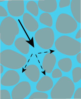
Figure 1: (Color online) The transport of tracer particles in a porous medium. This transport is regarded as noninteracting particles which undergo scatterings by scatterers.

The rest of the paper is organized as follows. In Sec. 2, the linear Boltzmann equation is introduced. We explore the advection-diffusion approximation in Sec. 3. In Sec. 4, we solve the linear Boltzmann equation. Section 5 is devoted to column experiments. Conclusions are given in Sec. 6.

2 Linear Boltzmann transport

The linear Boltzmann equation, radiative transport equation, or transport equation governs the transport of noninteracting particles with scattering and absorption. The equation describes neutron transport in a reactor (Case and Zweifel 1967) and light transport in random media such as clouds and the intersteller medium (Apresyan and Kravtsov 1996; Chandrasekhar 1960; Ishimaru 1978; Sovolev 1976; Thomas and Stamnes 1999). Let us regard the transport of tracer particles along flow paths as the transport of particles in a homogeneous random medium. See the schematic figure in Fig. 1. There is a random arrangement of flow paths in beads and sand in column experiments. At a branching point where several paths split into different directions, tracer particles are scattered to these directions with certain probabilities. The average distance that a tracer particle travels along a flow path between branching points is an effective mean free path $v_{0}/\sigma_{s}$ (see (1) for $v_{0},\sigma_{s}$). Indeed, the use of the linear Boltzmann equation for the flow of tracer particles in porous media was proposed by Williams (Williams 1992a, b, 1993a, 1993b).

A remark is necessary for our Boltzmann transport. The (nonlinear) Boltzmann equation can be simulated by the lattice Boltzmann scheme (Succi 2001), and the lattice Boltzmann method has become one of commonly used numerical methods to investigate the flow in porous media. Instead of fluid in porous media, we focus on the Boltzmann transport of tracer particles in the fluid. Hence, the proposed equation (1) below is a linear equation.

Having in mind the transport in column experiments which is described in Sec. 5, we consider the one-dimensional linear Boltzmann equation. Let $\mu\in[-1,1]$ be the cosine of the polar angle and $v_{0}>0$ be the inherent particle speed. Although the coefficient of the spatial derivative is $v_{0}\mu$ in Williams’ study (Williams 1992a, b) , in this paper, we take into account advection, which will be denoted by $u\geq 0$. Hence the velocity $v$ is written as $v=u+v_{0}\mu$. Let $\psi(x,\mu,t)$ be the angularly dependent number density of particles at position $x\geq 0$ in direction $\mu$ at time $t\geq 0$. We can write the linear Boltzmann equation as follows.

$$\frac{\partial}{\partial t}\psi(x,\mu,t)+(u+v_{0}\mu)\frac{\partial}{\partial x}\psi+(\sigma_{a}+\sigma_{s})\psi=\frac{\sigma_{s}}{2}\int^{1}_{-1}\psi(x,\mu,t)\,\mathrm{d}\mu.$$ (1)

where isotropic scattering is assumed in the integral on the right-hand side. Here, $\sigma_{a}\geq 0$ and $\sigma_{s}>0$ are the absorption and scattering coefficients, respectively. Let $n_{0}$ be the initial particle number density. Tracer particles are injected to the column at $x=0$ in the normal direction. The initial and boundary conditions are given by

$$\psi(x,\mu,0)=0,$$ (2)

$$\psi(0,\mu,t)=n_{0}\delta(\mu-1),\quad\mu>-\eta,$$ (3)

where $\delta(\mu-1)$ is the Dirac delta function and

$$\eta=\frac{u}{v_{0}}.$$ (4)

We note that unlike the usual half-range boundary condition of $\mu>0$ (Case and Zweifel 1967), the boundary value in (3) is specified for $\mu\in(-\eta,1]$ due to the presence of the advection. We regard the column as the half space ($0<x<\infty$) and have $\psi\to 0$ as $x\to\infty$.

The particle number density $n(x,t)$ is calculated as

$$n(x,t)=\int_{-1}^{1}\psi(x,\mu,t)\,\mathrm{d}\mu.$$ (5)

Then the concentration is given by

$$C(x,t)=\alpha n(x,t),$$ (6)

where $\alpha$ is the mass per particle.

3 Advection diffusion approximation

Let us derive the advection-diffusion equation from the linear Boltzmann equation. According the usual procedure of the diffusion approximation (Duderstadt and Martin 1979; Ishimaru 1978), we assume that the angular dependence of $\psi(x,\mu,t)$ is weak and written as

$$\psi(x,\mu,t)=\frac{1}{2\alpha}C(x,t)+\frac{3}{2\alpha v_{0}}J(x,t)\mu,$$ (7)

where,

$$C(x,t) =\alpha\int^{1}_{-1}\psi(x,\mu,t)\,\mathrm{d}\mu,$$ (8)

$$J(x,t) =\alpha v_{0}\int^{1}_{-1}\mu\psi(x,\mu,t)\,\mathrm{d}\mu.$$ (9)

In (7), we implicitly assumed a large propagation distance and long time. If absorption is strong, $\psi$ becomes zero before the form (7) is achieved. Hence we assume $\sigma_{a}$ is small. Indeed in Sec. 5, we will see that $\sigma_{a}$ is negligibly small. Indeed, the approximation in (7) is called the $P_{1}$ approximation (Case and Zweifel 1967). Below, we will proceed further and obtain the diffusion equation. We substitute the form (7) for $\psi$ in (1). By integrating the resulting equation over $\mu$, we obtain

$$\frac{\partial C}{\partial t}+u\frac{\partial C}{\partial x}+\frac{\partial J}{\partial x}+\sigma_{a}C=0.$$ (10)

By integrating the equation over $\mu$ after multiplying $\mu$, we obtain

$$\frac{1}{v_{0}}\frac{\partial J}{\partial t}+\frac{u}{v_{0}}\frac{\partial J}{\partial x}+\frac{v_{0}}{3}\frac{\partial C}{\partial x}+\frac{\sigma_{a}+\sigma_{s}}{v_{0}}J=0.$$ (11)

We assume that the first term and second term of the above equation are small and can be dropped. Then we have

$$J=-D\frac{\partial C}{\partial x},$$ (12)

where

$$D =\frac{v_{0}\ell^{*}}{3},$$ (13)

$$\ell^{*} =\frac{v_{0}}{\sigma_{a}+\sigma_{s}}\simeq\frac{v_{0}}{\sigma_{s}}.$$ (14)

Hence we obtain the following advection diffusion equation by substituting (12) into (10).

$$\frac{\partial C}{\partial t}-D\frac{\partial^{2}C}{\partial x^{2}}+u\frac{\partial C}{\partial x}+\sigma_{a}C=0,$$ (15)

For the photon diffusion equation, $\ell^{*}$ is known to be independent of the absorption coefficient (Furutsu and Yamada 1994). The diffusion approximation holds when $x$ is sufficiently larger than the transport mean free path $\ell^{*}$.

The diffusion equation (15) reduces to the usual advection-diffusion equation when $\sigma_{a}=0$. Since we found $\sigma_{a}\approx 0$ in our column experiments, the solution by Ogata and Banks (Ogata and Banks 1961) is used in this paper when the concentration calculated from the linear Boltzmann equation is compared to the advection-diffusion equation. In Appendix B, the solution to (15) is presented.

Finally, we consider the boundary condition. Let us substitute (7) for $\psi(x,\mu,t)$ in the boundary condition (3). By integrating both sides of the resulting equation over $\mu$ from $-\eta$ to $1$, we obtain

$$C(0,t)-\frac{3D\eta(1-\eta)}{2}\frac{D}{u}\frac{\partial C}{\partial x}(0,t)=\frac{2\alpha n_{0}}{1+\eta}.$$ (16)

Thus we obtain the Robin boundary condition. In this paper, we neglect the flux term and write

$$C(0,t)=C_{0},$$ (17)

where $C_{0}>0$ denotes the boundary source. Since the diffusion approximation does not hold on the boundary, the actual proportionality constant between $\alpha n_{0}$ and $C_{0}$ is a fitting parameter. We introduce

$$\beta=\frac{\alpha n_{0}}{C_{0}}.$$ (18)

4 Concentration from the linear Boltzmann equation

Let us consider the Laplace transform.

$$\hat{\psi}(x,\mu,p)=\int^{\infty}_{0}\mathrm{e}^{-pt}\psi(x,\mu,t)\,\mathrm{d}t.$$ (19)

We introduce

$$\mu_{t}=\frac{\sigma_{a}+\sigma_{s}+p}{v_{0}},\quad\mu_{s}=\frac{\sigma_{s}}{v_{0}}.$$ (20)

Then our transport equation is written as

$$(\eta+\mu)\frac{\partial}{\partial x}\hat{\psi}(x,\mu,p)+\mu_{t}\hat{\psi}(x,\mu,p)=\frac{\mu_{s}}{2}\int^{1}_{-1}\hat{\psi}(x,\mu,p)\,\mathrm{d}\mu,$$ (21)

with the boundary condition,

$$\hat{\psi}(0,\mu,p)=\frac{n_{0}}{p}\delta(\mu-1),\quad\mu>-\eta.$$ (22)

We will compute $\hat{\psi}$ with the analytical discrete ordinates method (ADO) (Siewert and Wright 1999; Barichello et al. 2000; Barichello and Siewert 2001). Unlike the standard ADO, the coefficient $\mu_{t}$ is a complex number since the variable $p$ is complex and moreover, the boundary condition is given for $\mu>-\eta$ instead of $\mu>0$. We begin by decomposing $\hat{\psi}$ into the ballistic term $\hat{\psi}_{b}$ and scattering term $\hat{\psi}_{s}$ as

$$\hat{\psi}(x,\mu,p)=\hat{\psi_{b}}(x,\mu,p)+\hat{\psi_{s}}(x,\mu,p).$$ (23)

Here, $\hat{\psi}_{b}$ obeys

$$(\eta+\mu)\frac{\partial}{\partial x}\hat{\psi_{b}}+\mu_{t}\hat{\psi_{b}}=0,\quad x>0,\;-1\leq\mu\leq 1,$$ (24)

with the boundary condition

$$\hat{\psi_{b}}(0,\mu,p)=\frac{n_{0}}{p}\delta(\mu-1),\quad\mu>-\eta,$$ (25)

and $\hat{\psi}_{s}$ obeys

$$(\eta+\mu)\frac{\partial}{\partial x}\hat{\psi_{s}}+\mu_{t}\hat{\psi_{s}}=\frac{\mu_{s}}{2}\int^{1}_{-1}\hat{\psi_{s}}\,\mathrm{d}\mu+q,\quad x>0,\;-1\leq\mu\leq 1,$$ (26)

with the boundary condition

$$\hat{\psi_{s}}(0,\mu,p)=0,\quad\mu>-\eta,$$ (27)

where

$$q(x,\mu,p)=\frac{\mu_{s}}{2}\int^{1}_{-1}\hat{\psi_{b}}(x,\mu,p)\,\mathrm{d}\mu=\frac{n_{0}\mu_{s}}{2p}\mathrm{e}^{-x\mu_{t}/(\eta+\mu)}.$$ (28)

We obtain

$$\hat{\psi_{b}}(x,\mu,p)=\frac{n_{0}}{p}\mathrm{e}^{-x\mu_{t}/(\eta+\mu)}\delta(\mu-1).$$ (29)

Let us drop $p$ and write $\hat{\psi}_{s}(x,\mu)=\hat{\psi}_{s}(x,\mu,p)$ and $q(x,\mu)=q(x,\mu,p)$. For the computation of $\hat{\psi}_{s}$, we discretize the integral by the Gauss-Legendre quadrature and obtain

$$(\eta+\mu_{i})\frac{\partial}{\partial x}\hat{\psi_{s}}(x,\mu_{i})+\mu_{t}\hat{\psi_{s}}(x,\mu_{i})$$

$$=\frac{\mu_{s}}{2}\sum^{N}_{j=1}w_{j}\left[\hat{\psi_{s}}(x,\mu_{j})+\hat{\psi_{s}}(x,-\mu_{j})\right]+q(x,\mu_{i}),$$ (30)

where $\mu_{i},w_{i}$ ($i=1,2,\dots,2N$) are abscissas and weights, respectively. These $\mu_{i},w_{i}$ with $0<\mu_{1}<\cdots<\mu_{N}<1$ and $\mu_{N+i}=-\mu_{i}$ ($i=1,\dots,N$) can be calculated by the Golub-Welsch algorithm (Golub and Welsch 1969). In the numerical calculation in Sec. 5, we set

$$N=30.$$ (31)

Furthermore, we introduce $N_{\eta}$ as the largest integer such that $-\eta<\mu_{N_{\eta}}$. The scattering part $\hat{\psi}_{s}$ is obtained as

$$\hat{\psi_{s}}(x,\mu_{i})=\sum^{2N}_{j=1}\int^{\infty}_{0}G(x,\mu_{i};x^{\prime},\mu_{j})q(x^{\prime},\mu_{j})\,\mathrm{d}x^{\prime},$$ (32)

where the Green’s function defined for each $p$ satisfies

$$(\eta+\mu_{i})\frac{\partial}{\partial x}G(x,\mu_{i};x_{0},\mu_{i_{0}})+\mu_{t}G(x,\mu_{i};x_{0},\mu_{i_{0}}) =\frac{\mu_{s}}{2}\sum^{2N}_{j=1}w_{j}G(x,\mu_{j};x_{0},\mu_{i_{0}})$$

$$+\delta(x-x_{0})\delta_{ii_{0}},$$ (33)

where $\delta_{ii_{0}}$ is the Kronecker delta. Here the boundary condition is given by

$$G(0,\mu_{i};x_{0},\mu_{i_{0}})=0,\quad\mu_{i}>\mu_{N_{\eta}}.$$ (34)

Let us consider the following homogeneous equation to calculate the Green’s function with ADO (Siewert and Wright 1999; Barichello et al. 2000; Barichello and Siewert 2001). Note that the equation will be solved for each $p$.

$$\left((\eta+\mu_{i})\frac{\partial}{\partial x}+\mu_{t}\right)\hat{\psi}(x,\mu_{i})=\frac{\mu_{s}}{2}\sum^{2N}_{j=1}w_{j}\hat{\psi}(x,\mu_{j}).$$ (35)

We note that $\hat{\psi}$ depends on $p$ through $\mu_{t}$. With separation of variables, we can write $\hat{\psi}$ as

$$\hat{\psi}(x,\mu_{i})=\phi(\nu,\mu_{i})\mathrm{e}^{-x/\nu},$$ (36)

where $\nu$ is the separation constant. The function $\phi(\nu,\mu_{i})$ satisfies the normalization condition,

$$\sum^{2N}_{i=1}w_{i}\phi(\nu,\mu_{i})=\sum^{N}_{i=1}w_{i}\left(\phi(\nu,\mu_{i})+\phi(\nu,-\mu_{i})\right)=1.$$ (37)

For the integral equation in which the sum on the right-hand side of (35) is replaced by the integral $\frac{\mu_{s}}{2}\int_{-1}^{1}\hat{\psi}\,\mathrm{d}\mu$, this $\phi$ is called the singular eigenfunction (Case 1960). However, by the discretization, we obtain

$$\phi(\nu,\mu_{i})=\frac{\mu_{s}\nu}{2}\frac{1}{\mu_{t}\nu-\mu_{i}-\eta}.$$ (38)

assuming $\nu\neq(\mu_{i}+\eta)/\mu_{t}$. It is known that $\mu\neq\mu_{i}/\mu_{t}$ if $\eta=0$ and $p$ is real (Siewert and Wright 1999). We can show the following orthogonality relation.

$$\sum^{2N}_{i=1}w_{i}(\mu_{i}+\eta)\phi(\nu,\mu_{i})\phi(\nu^{\prime},\mu_{i})=\mathcal{N}(\nu)\delta_{\nu\nu^{\prime}},$$ (39)

where

$$\mathcal{N}(\nu)=\sum^{2N}_{i=1}w_{i}(\mu_{i}+\eta)\phi(\nu,\mu_{i})^{2}.$$ (40)

We can find $2N$ eigenvalues $\nu=\nu_{n}$ ($n=1,2,\dots,2N$). Moreover there are $N_{\eta}$ eigenvalues with positive real parts. See Appendix A for the eigenvalues.

Taking the fact that $G$ vanishes as $x\to\infty$, we can write

$$G(x,\mu_{i};x_{0},\mu_{i_{0}}) =G_{0}(x,\mu_{i};x_{0},\mu_{i_{0}})$$

$$+\sum_{\Re{\nu_{n}}>0}B(\nu;x_{0},\mu_{i_{0}})\phi(\nu,\mu_{i})\mathrm{e}^{-x/\nu},$$ (41)

where coefficients $B(\nu;x_{0},\mu_{i_{0}})$ will be determined later. The free-space Green’s function $G_{0}$ is calculated as

$$G_{0}(x,\mu_{i};x_{0},\mu_{i_{0}})=\pm\sum_{\pm\Re{\nu_{n}}>0}\frac{w_{i_{0}}}{\mathcal{N}(\nu_{n})}\phi(\nu_{n},\mu_{i_{0}})\phi(\nu_{n},\mu_{i})\mathrm{e}^{-(x-x_{0})/\nu_{n}},$$ (42)

where upper signs are chosen for $x>x_{0}$ and lower signs are used for $x<x_{0}$. Since $G$ vanishes at $x=0$ for $\mu_{i}>\mu_{N_{\eta}}$, we have from (4),

$$\sum_{\Re{\nu_{n}}>0}B(\nu;x_{0},\mu_{i_{0}})\phi(\nu_{n},\mu_{i})=\sum_{\Re{\nu_{n}}<0}\frac{w_{i_{0}}}{\mathcal{N}(\nu_{n})}\phi(\nu_{n},\mu_{i_{0}})\phi(\nu_{n},\mu_{i})\mathrm{e}^{x_{0}/\nu_{n}}.$$ (43)

Let us multiply (43) by $\exp(-x_{0}\mu_{t}/(\eta+1))$, then integrate both sides with $x_{0}$ and take the sum with respect to $i$. We obtain

$$\sum_{\Re{\nu_{n}}>0}E(\nu_{n})\phi(\nu_{n},\mu_{i})=\sum_{\Re{\nu_{n}}<0}\frac{-\nu_{n}(\eta+1)}{\mathcal{N}(\nu_{n})(\eta+1-\nu_{n}\mu_{t})}\phi(\nu_{n},\mu_{i}),$$ (44)

where

$$E(\nu_{n})=\sum_{i_{0}=1}^{2N}\int_{0}^{\infty}B(\nu_{n};x_{0},\mu_{i_{0}})\mathrm{e}^{-\mu_{t}x_{0}/(\eta+1)}\,\mathrm{d}x_{0}.$$ (45)

We can numerically obtain $E(\nu_{n})$ from the linear system (44). Finally, we obtain

$$\hat{\psi_{s}}(x,\mu_{i}) =\frac{n_{0}\mu_{s}}{2p}\sum_{\Re{\nu_{n}}>0}\left[\frac{\nu_{n}}{\mathcal{N}(\nu_{n})}\phi(\nu_{n},\mu_{i})\frac{\eta+1}{\eta+1-\nu_{n}\mu_{t}}\left(\mathrm{e}^{-\mu_{t}x/(\eta+1)}-\mathrm{e}^{-x/\nu_{n}}\right)\right]$$

$$+\frac{n_{0}\mu_{s}}{2p}\sum_{\Re{\nu_{n}}<0}\left[\frac{\nu_{n}}{\mathcal{N}(\nu_{n})}\phi(\nu_{n},\mu_{i})\frac{\eta+1}{\eta+1-\nu_{n}\mu_{t}}\mathrm{e}^{-\mu_{t}x/(\eta+1)}\right]$$

$$+\frac{n_{0}\mu_{s}}{2p}\sum_{\Re{\nu_{n}}>0}E(\nu_{n})\phi(\nu_{n},\mu_{i})\mathrm{e}^{-x/\nu_{n}}.$$ (46)

In this way, $\hat{\psi}_{s}$ is computed using ADO.

The Laplace transform of the particle number density $\hat{n}(x,p)$ is obtained as

$$\hat{n}(x,p) =\int^{1}_{-1}\hat{\psi}(x,\mu,p)\,\mathrm{d}\mu$$

$$=\int^{1}_{-1}\hat{\psi_{b}}(x,\mu,p)\,\mathrm{d}\mu+\int^{1}_{-1}\hat{\psi_{s}}(x,\mu,p)\,\mathrm{d}\mu$$

$$=\frac{n_{0}}{p}\mathrm{e}^{-x\mu_{t}/(\eta+1)}$$

$$+\frac{n_{0}\mu_{s}}{2p}\sum_{\Re{\nu_{n}}>0}\left[\frac{\nu_{n}}{\mathcal{N}(\nu_{n})}\frac{\eta+1}{\eta+1-\nu_{n}\mu_{t}}\left(\mathrm{e}^{-x\mu_{t}/(\eta+1)}-\mathrm{e}^{-x/\nu_{n}}\right)\right]$$

$$+\frac{n_{0}\mu_{s}}{2p}\sum_{\Re{\nu_{n}}<0}\left[\frac{\nu_{n}}{\mathcal{N}(\nu_{n})}\frac{\eta+1}{\eta+1-\nu_{n}\mu_{t}}\mathrm{e}^{-x\mu_{t}/(\eta+1)}\right]$$

$$+\frac{n_{0}\mu_{s}}{2p}\sum_{\Re{\nu_{n}}>0}E(\nu_{n})\mathrm{e}^{-x/\nu_{n}}.$$ (47)

We note that the particle number density $n(x,t)$ is given by

$$n(x,t)=\frac{1}{2\pi\mathrm{i}}\int^{\gamma+\mathrm{i}\infty}_{\gamma-\mathrm{i}\infty}\mathrm{e}^{pt}\hat{n}(x,p)\,\mathrm{d}p.$$ (48)

The Bromwich integral in the inverse Laplace transform is numerically evaluated by the trapezoidal rule. In general, deformation of the contour can be considered for the inversion (Weideman and Trefethen 2007). We found $\gamma=0.04$ is suitable. Hence, the concentration is obtained as

$$C(x,t) =\frac{\alpha n_{0}\mu_{s}}{4\pi\mathrm{i}}\int^{\gamma+\mathrm{i}\infty}_{\gamma-\mathrm{i}\infty}\frac{\mathrm{e}^{pt}}{p}\Biggl{\{}\frac{2}{\mu_{s}}\mathrm{e}^{-x\mu_{t}/(\eta+1)}$$

$$+\sum_{\Re{\nu_{n}}>0}\left[\frac{\nu_{n}}{\mathcal{N}(\nu_{n})}\frac{\eta+1}{\eta+1-\nu_{n}\mu_{t}}\left(\mathrm{e}^{-x\mu_{t}/(\eta+1)}-\mathrm{e}^{-x/\nu_{n}}\right)\right]$$

$$+\sum_{\Re{\nu_{n}}<0}\left[\frac{\nu_{n}}{\mathcal{N}(\nu_{n})}\frac{\eta+1}{\eta+1-\nu_{n}\mu_{t}}\mathrm{e}^{-x\mu_{t}/(\eta+1)}\right]$$

$$+\sum_{\Re{\nu_{n}}>0}E(\nu_{n})\mathrm{e}^{-x/\nu_{n}}\Biggr{\}}\,\mathrm{d}p.$$ (49)

5 Column experiments

Column experiments are often used for the study of transport in random media (Cortis 2004). We here present results of a series of tracer breakthrough experiments conducted in a one-dimensional flow field. Fluid with tracer particles is injected by the peristaltic pump (MP-1000, Eyela). The flow rate of injected tracer solution is controlled by the peristaltic pump. Ultra pure water is used. First, water is injected for 24 hours or more until steady flow field is achieved. Next, tracer solution is injected to displace the fresh water. The discharged solution is collected by the fraction collector (CHF161RA, Advantec) at regular intervals. Column experiments are performed at room temperature of $25$–$26\,{}^{\circ}{\rm C}$.

Tracer experiments are conducted until the discharge concentration becomes equal to the influent concentration. For the sake of the accuracy of measurements, we correct the measurement time error from the tube volume and inlet volume of the column by subtracting the time lag due to the switchover from the breakthrough time.

5.1 Column experiments with non-adsorbed solute

First we use non-adsorbed solute. We use two different sizes of glass beads made with Soda glass; (Run 1) smaller beads with diameter ranging from $0.177\,{\rm mm}$ to $0.250\,{\rm mm}$ and (Run 2) larger beads with diameter from $0.500\,{\rm mm}$ to $0.710\,{\rm mm}$. The column length is $20.0\,{\rm cm}$ with the internal diameter of the column $2.9\,{\rm cm}$. In order to prevent entrainment of air, we carry out beads packing under saturated conditions, in which the water surface is kept at a constant height from the top of the beads layer. We stirrer beads while filling in order to remove small bubbles attached to the beads.

The inlet and the outlet ends of the column are separated from the porous medium of a glass filter with the pore size $10\,{\rm\mu m}$, originally for the purpose of the liquid chromatography. The glass filter serves to enhance tracer mixing and to dampen small flow pulses on injection. The tracer concentration is measured by the EC meter (LAQUAtwin-EC-33B, Horiba). The precision of the meter is $\pm 2\%$. The temperature compensation circuit is installed.

We prepare the NaCl solution of $0.1\%$ with the salt of purity $99.5\%$ (Wako). Injection of the solution is done by the peristaltic pump. The measured EC values are given by the unit of Sv/cm, we made the calibration curve and obtain the concentration.

5.1.1 Run 1: small beads

The column is filled with small beads. The measured porosity is $\eta=0.386$. The bed height is $18.0\,{\rm cm}$ with section area $6.61\,{\rm cm}^{2}$. The flow rate is $0.958\,{\rm cm}^{3}/{\rm min}$.

Figure 2 shows the chloride breakthrough curve from Run 1. The vertical axis shows the relative concentration $C/C_{0}$ and the horizontal axis is time $t$. The measured values from the column experiment (black dots) are compared to $C/C_{0}$ calculated by the linear Boltzmann equation (LBE) (red solid line) and by the ADE model (Ogata and Banks 1961) (blue dashed line). The parameters in both equations are determined by nonlinear least-squares fitting (i.e., the minimization of the sum of squares of the residuals between the experimental and theoretical curves); they are obtained as $\sigma_{a}=1.0\times 10^{-8}\,{\rm min}^{-1}$, $\sigma_{s}=5.1645\,{\rm min}^{-1}$, $v_{0}=5.3073\,{\rm cm}/{\rm min}$, $u=1.6445\,{\rm cm}/{\rm min}$, $\beta=0.09130$ for LBE, and $u=1.2886\,{\rm cm}/{\rm min}$, $D=1.8379\,{\rm cm}^{2}/{\rm min}$ for ADE. In Fig. 2, experimental results agree well with both LBE and ADE. Figure 3 shows semi-log plots of $1-C/C_{0}$ as a function of $t$.

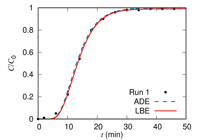
Figure 2: (Color online) The relative concentration $C/C_{0}$ for Run 1 (black dots) is plotted with calculated values from LBE (red solid line) and ADE (blue dashed line).

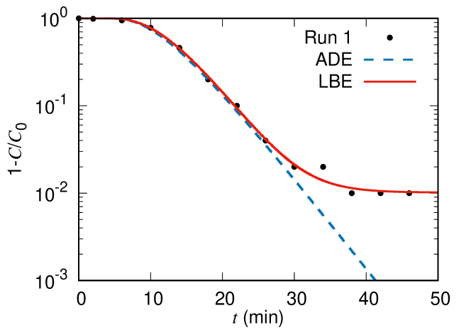
Figure 3: (Color online) Same as Fig. 2 but $1-C/C_{0}$ is plotted in the semi-log graph.

5.1.2 Run 2: large beads

The column is filled with large beads. The measured porosity is $\eta=0.367$. (This value of the porosity is smaller than that of Run 1. This may be due to small bubbles attached on the beads surface during Run 1.) The bed height is $18.5\,{\rm cm}$ with section area $6.61\,{\rm cm}^{2}$. The flow rate is $0.875\,{\rm cm}^{3}/{\rm min}$.

Figure 4 for Run 2 is the same as Fig. 2 but large glass beads are used. By nonlinear least-squares fitting, the parameters are obtained as $\sigma_{a}=1.0\times 10^{-8}\,{\rm min}^{-1}$, $\sigma_{s}=4.6778\,{\rm min}^{-1}$, $v_{0}=8.1753\,{\rm cm}/{\rm min}$, $u=2.4999\,{\rm cm}/{\rm min}$, $\beta=0.08579$ for LBE, and $u=1.6189\,{\rm cm}/{\rm min}$, $D=3.8519\,{\rm cm}^{2}/{\rm min}$ for ADE. In Fig. 4, experimental results are described well by LBE and ADE. The long-time behavior is shown in Fig. 5, in which $1-C/C_{0}$ is plotted.

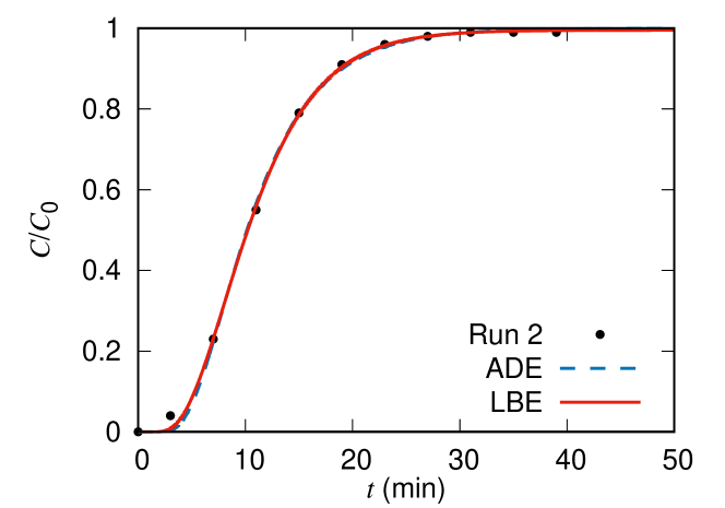
Figure 4: (Color online) The relative concentration $C/C_{0}$ for Run 2 (black dots) is plotted with calculated values from LBE (red solid line), and ADE (blue dashed line).

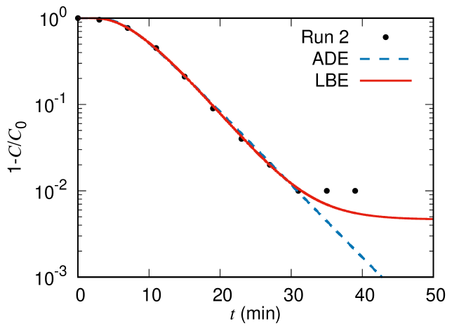
Figure 5: (Color online) Same as Fig. 4 but $1-C/C_{0}$ is plotted in the semi-log graph.

5.2 Column experiments with adsorbed solute

Here we use adsorptive solute (zinc solution). The filling material is the standard sand (Tohoku silica sand No. 4, Kitanihon Sangyo). The median diameter of the sand is 750$\mu$m. As a preparation, we eliminate the organic matter that may have been contained in the sand by soaking it in ${\rm HNO}_{3}$ solution. The zinc solution is 2 ppm. We set a filter on the top of the sand bed made with glass wool. We also put the same filter at the bottom of the column.

A short column of length $12.0\,{\rm cm}$ with internal diameter $3.1\,{\rm cm}$ was used. We perform a blank test beforehand to make sure that the zinc is not absorbed on the surface of the column wall. The concentration is measured with the atomic absorption photometer (Z-2300, Hitachi High-Technologies), the compressor (SC820, Koki Holdings), and the neo cool circulator (CF700, Yamato).

5.2.1 Run 3

The measured porosity is $0.295$ and the flow rate is $9.34\,{\rm cm}^{3}/{\rm h}$. The bed height is $10.7\,{\rm cm}$ and the section area is $7.54\,{\rm cm}^{2}$.

Figure 6 shows the relative concentration $C/C_{0}$ of the zinc breakthrough curve for Run 3 (black dots) with calculated values from the linear Boltzmann equation (LBE) (red solid line) and the Ogata-Banks ADE model (blue dashed line). By nonlinear least-squares fitting, we obtain $\sigma_{a}=1.0\times 10^{-7}\,{\rm h}^{-1}$, $\sigma_{s}=2.8134\,{\rm h}^{-1}$, $v_{0}=5.0663\,{\rm cm}/{\rm h}$, $u=1.9876\,{\rm cm}/{\rm h}$, $\beta=0.1739$ for LBE, and $u=1.1406\,{\rm cm}/{\rm h}$, $D=4.3864\,{\rm cm}^{2}/{\rm h}$. The dashed curve for ADE partially deviates from the measured values. The semi-log plot in Fig. 7 shows a clear discrepancy between the experimental result and ADE.

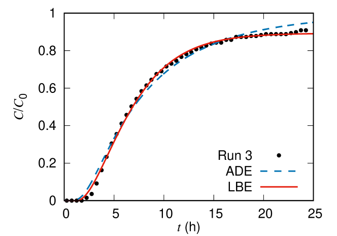
Figure 6: The relative concentration $C/C_{0}$ for Run 3 (black dots) is plotted with calculated values by LBE (red solid line) and by ADE (blue dashed line).

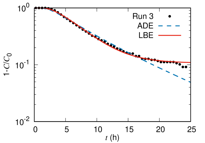
Figure 7: Same as Fig. 6 but $1-C/C_{0}$ is plotted in the semi-log graph.

5.2.2 Run 4

Figure 8 for Run 4 is the same as Fig. 6 but we repeat another run for the standard sand and adsorbed solute. The measured porosity is $0.289$ and the flow rate is $11.25\,{\rm cm}^{3}/{\rm h}$. The bed height is $10.7\,{\rm cm}$ and the section area is $7.54\,{\rm cm}^{2}$. By nonlinear least-squares fitting, we obtain $\sigma_{a}=1.0\times 10^{-7}\,{\rm h}^{-1}$, $\sigma_{s}=2.6773\,{\rm h}^{-1}$, $v_{0}=4.1166\,{\rm cm}/{\rm h}$, $u=1.7999\,{\rm cm}/{\rm h}$, $\beta=0.2091$ for LBE, and $u=1.1384\,{\rm cm}/{\rm h}$, $D=3.9814\,{\rm cm}^{2}/{\rm h}$ for ADE. The discrepancy of ADE is even more apparent. The semi-log plot in Fig. 9 shows a discrepancy between the experimental result and ADE.

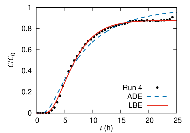
Figure 8: The relative concentration $C/C_{0}$ for Run 4 (black dots) is plotted with calculated values by LBE (red solid line) and by ADE (blue dashed line).

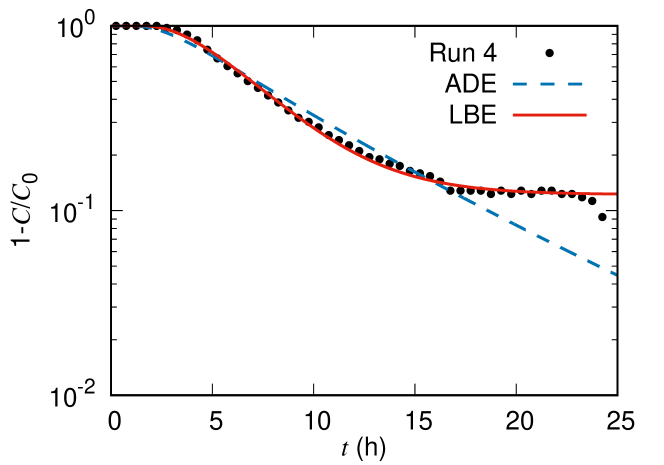
Figure 9: Same as Fig. 8 but $1-C/C_{0}$ is plotted in the semi-log graph.

6 Conclusions

Not only for field observation reported in studies such as Adams and Gelhar (Adams and Gelhar 1992) and Benson and his collaborators (Benson et al. 2001, 2000), anomalous diffusion also appears in lab-scale experiments (Cortis 2004). In Sec. 5, ADE does not precisely reproduce the breakthrough curves even for beads, which form a medium material with non-adsorbed solution. Williams proposed to use the linear Boltzmann equation for transport in porous media (Williams 1992a, b, 1993a, 1993b). It was shown that the proposed model of the linear Boltzmann equation reproduces the whole breakthrough curves of experimental results including the non-monotonic decay of $1-C/C_{0}$ in the tail.

The diffusion approximation holds when the propagation distance of tracer particles is sufficiently larger than the transport mean free path $\ell^{*}$, which is given in (14). In the case of light transport, the photon diffusion equation starts to work when the propagation distance becomes $10$ times larger than the transport mean free path (Yoo et al. 1990). Using the relation (13), we can calculate the diffusion coefficient, which is denoted by $D^{\prime}$, from parameters in the linear Boltzmann equation. We let $D$ denote the fitted diffusion coefficient in the advection-diffusion equation. Let us compare Run 1 and Run 2. For Run 1 in Sec. 5.1.1, $\ell^{*}=1.03$ and $D^{\prime}=1.818$, whereas $D=1.8379$. The relative difference is $|D-D^{\prime}|/D=0.0108$. For Run 2 in Sec. 5.1.2, $\ell^{*}=1.75$ and $D^{\prime}=4.762$, whereas $D=3.8519$. The relative difference is $|D-D^{\prime}|/D=0.236$. In either case, the propagation distance of $18\,{\rm cm}$ or $18.5\,{\rm cm}$ is much larger than $\ell^{*}$ and the transport is expected to be in the diffusion regime. Indeed, Fig. 2 and Fig. 4 show that both LBE and ADE reproduce the experimentally obtained breakthrough curves. Next, let us also look at Run 3 and Run 4. For Run 3 in Sec. 5.2.1, $\ell^{*}=1.80$ and $D^{\prime}=3.041$, whereas $D=4.3864$. The relative difference is $|D-D^{\prime}|/D=0.307$. For Run 4 in Sec. 5.2.2, $\ell^{*}=1.54$ and $D^{\prime}=2.110$, whereas $D=3.9814$. The relative difference is $|D-D^{\prime}|/D=0.470$. The propagation distance of $10.7\,{\rm cm}$ is not as long as the distance in Run 1 and Run 2 in terms of the transport mean free path. The discrepancy of the curve for ADE in Fig. 6 and Fig. 8 might also attribute to anisotropic scattering for the sand. The transport mean free path becomes larger when the scattering in LBE becomes anisotropic. Moreover the discrepancy may come from the fact that the surface of the sand is rough and the particle speed cannot be modeled by a constant $v_{0}$.

Although we assumed isotropic scattering in (1), it is possible to take anisotropic scattering into account and write the integral term in a more general form as $\sigma_{s}\int_{-1}^{1}p(\mu,\mu^{\prime})\psi(x,\mu^{\prime},t)\,\mathrm{d}\mu^{\prime}$, where $p(\mu,\mu^{\prime})$ is the probability that tracer particles moving in the direction $\mu^{\prime}$ change their direction to the direction $\mu$ by scattering. We can similarly develop the analytical discrete ordinates method for anisotropic scattering by writing $p(\mu,\mu^{\prime})=\frac{1}{2}\sum_{l}\beta_{l}P_{l}(\mu)P_{l}(\mu^{\prime})$ with some constant coefficients $\beta_{l}$ and Legendre polynomials $P_{l}$ ($l=0,1,\dots$) (Barichello 2011; Siewert 2000).

In this paper we have shown that the mass transport in column experiments, which show anomalous diffusion, obeys the linear Boltzmann equation. Furthermore the linear Boltzmann equation in the transport regime appears at the mesoscopic scale and the advection-diffusion equation in the diffusion regime is derived from the linear Boltzmann equation in the asymptotic limit when the propagation distance is sufficiently larger than $\ell^{*}$ at the macroscopic scale. The physical origin of anomalous diffusion in a heterogeneous random medium with more complex structure of fissures is still an open problem.

Appendix A Eigenvalues

Let us write the homogeneous equation as

$$\left(\mu_{t}I-\frac{1}{\nu}\Xi_{+}\right)\Phi_{+} =\frac{\mu_{s}}{2}W\left(\Phi_{+}+\Phi_{-}\right),$$ (50)

$$\left(\mu_{t}I-\frac{1}{\nu}\Xi_{-}\right)\Phi_{-} =\frac{\mu_{s}}{2}W\left(\Phi_{+}+\Phi_{-}\right),$$

where $I$ is the identity, $\Xi_{\pm}$ and $W$ are matrices, and $\Phi_{\pm}$ are vectors defined as

$$\Xi_{\pm}=\begin{pmatrix}\pm\mu_{1}+\eta&&&\\ &\pm\mu_{2}+\eta&&\\ &&\ddots&\\ &&&\pm\mu_{N}+\eta\end{pmatrix},\quad\Phi_{\pm}=\begin{pmatrix}\phi(\nu,\pm\mu_{1})\\ \phi(\nu,\pm\mu_{2})\\ \vdots\\ \phi(\nu,\pm\mu_{N})\end{pmatrix},\quad\left\{W\right\}_{ij}=w_{j}.$$ (51)

We obtain

$$SM\begin{pmatrix}\Phi_{+}\\ \Phi_{-}\end{pmatrix}=\frac{1}{\nu}\begin{pmatrix}\Phi_{+}\\ \Phi_{-}\end{pmatrix},$$ (52)

where

$$S=\begin{pmatrix}\Xi_{+}^{-1}&\\ &\Xi_{-}^{-1}\end{pmatrix},\quad M=\mu_{t}(s)\begin{pmatrix}I&\\ &I\end{pmatrix}-\frac{\mu_{s}}{2}\begin{pmatrix}W&W\\ W&W\end{pmatrix}.$$ (53)

We label the eigenvalues as $\nu_{n}$ ($n=1,2,\dots,2N$).

By deforming the Bromwich contour, we obtain a contour $(-\infty,\gamma)$, $\gamma>0$, on which $s$ is real. In this case we have

$$SMw_{0}=\lambda_{0}w_{0},$$ (54)

where $\lambda_{0}$ is real and $w_{0}$ a $2N$-dimensional real vector. We note that $M=\Re{M}$ in this case and moreover we can write

$$\mu_{t}(s)=\frac{\sigma_{a}+\sigma_{s}+\Re{s}}{v_{0}}.$$ (55)

Since $M$ is a symmetric real matrix, by the Cholesky decomposition we can write $M=U^{T}U$, where $U$ is a real triangular matrix with positive diagonal entries. Hence,

$$USU^{T}\widetilde{w_{0}}=\lambda\widetilde{w_{0}},\quad\widetilde{w_{0}}=Uw_{0}.$$ (56)

Since $U$ is nonsingular, $S$ and $USU^{T}$ have the same inertia, i.e., the same number of positive, negative, and zero eigenvalues according to Sylvester’s law of inertia. Clearly, $S$ has $N_{\eta}$ positive eigenvalues. Therefore there are $N_{\eta}$ eigenvalues $\lambda_{0}$.

Next we assume that $s$ has a small imaginary part. Then we can write

$$S\left(\Re{M}+i\frac{\Im{s}}{v_{0}}\begin{pmatrix}I&\\ &I\end{pmatrix}\right)w=\lambda w.$$ (57)

We treat the imaginary part as perturbation and express the matrix-vector equation as

$$S\left(\Re{M}+i\epsilon\frac{\Im{s}}{v_{0}}\begin{pmatrix}I&\\ &I\end{pmatrix}\right)\left(w_{0}+\epsilon w_{1}+\cdots\right)=\left(\lambda_{0}+\lambda_{1}+\cdots\right)\left(w_{0}+\epsilon w_{1}+\cdots\right).$$ (58)

By collecting terms of order $O(\epsilon^{0})$, we have $S(\Re{M})w_{0}=\lambda_{0}w_{0}$. From terms of $O(\epsilon^{1})$, we have

$$S(\Re{M})w_{1}+i\frac{\Im{s}}{v_{0}}Sw_{0}=\lambda_{0}w_{1}+\lambda_{1}w_{0}.$$ (59)

Let us multiply $w_{0}^{T}$ on both sides of the above equation. We obtain

$$w_{0}^{T}S(\Re{M})w_{1}+i\frac{\Im{s}}{v_{0}}w_{0}^{T}Sw_{0}=\lambda_{0}w_{0}^{T}w_{1}+\lambda_{1}w_{0}^{T}w_{0}.$$ (60)

Using $w_{0}^{T}(S(\Re{M}))^{T}=w_{0}^{T}S\Re{M}=\lambda_{0}w_{0}^{T}$, we obtain

$$\lambda_{1}=i\frac{(\Im{s})w_{0}^{T}Sw_{0}}{v_{0}w_{0}^{T}w_{0}}.$$ (61)

That is, $\lambda_{1}$ is pure imaginary and the number of positive $\Re{\lambda}$ does not change. This fact implies that there are $N_{\eta}$ eigenvalues $\nu_{n}$ ($n=1,\dots,2N$) such that $\Re{\nu_{n}}>0$.

Appendix B Advection-diffusion equation with absorption

Let us consider the following advection-diffusion equation with the absorption term.

$$\left(\frac{\partial}{\partial t}-D\frac{\partial^{2}}{\partial x^{2}}+u\frac{\partial}{\partial x}+\sigma_{a}\right)C(x,t)=0,$$ (62)

$$C(x,0)=0,$$ (63)

$$C(0,t)=C_{0}.$$ (64)

Let us introduce $\Gamma(x,t)$ as

$$C(x,t)=\Gamma(x,t)\exp\left(\frac{ux}{2D}-\frac{u^{2}t}{4D}-\sigma_{a}t\right).$$ (65)

We have

$$\frac{\partial}{\partial t}\Gamma(x,t)-D\frac{\partial^{2}}{\partial x^{2}}\Gamma(x,t)=0,$$ (66)

$$\Gamma(x,0)=0,$$ (67)

$$\Gamma(0,t)=C_{0}\exp\left(\frac{u^{2}t}{4D}+\sigma_{a}t\right).$$ (68)

Let us consider the Laplace transform:

$$\hat{\Gamma}(x,p)=\int_{0}^{\infty}\mathrm{e}^{-pt}\Gamma(x,t)\,\mathrm{d}t,\quad\Re{p}>\frac{u^{2}}{4D}+\sigma_{a}.$$ (69)

Then we obtain

$$\frac{\partial^{2}}{\partial x^{2}}\hat{\Gamma}(x,p)=\frac{p}{D}\hat{\Gamma}(x,p),\quad\hat{\Gamma}(0,p)=\frac{C_{0}}{p-\frac{u^{2}}{4D}-\sigma_{a}}.$$ (70)

We obtain

$$\hat{\Gamma}(x,p)=\frac{C_{0}}{p-\frac{u^{2}}{4D}-\sigma_{a}}\mathrm{e}^{-\sqrt{\frac{p}{D}}x}.$$ (71)

Thus,

$$\Gamma(x,t)=C_{0}\int_{0}^{t}f(t-\tau)g(\tau)\,d\tau,$$ (72)

where

$$\hat{f}(p)=\frac{1}{p-\frac{u^{2}}{4D}-\sigma_{a}},\quad\hat{g}(p)=\mathrm{e}^{-\sqrt{\frac{p}{D}}x}.$$ (73)

Noting that

$$\int_{0}^{\infty}\mathrm{e}^{-pt}e^{at}\,\mathrm{d}t=\frac{1}{p-a}\;(\Re{p}>a),\quad\int_{0}^{\infty}\mathrm{e}^{-pt}\frac{b}{2\sqrt{\pi}t^{3/2}}e^{-\frac{b^{2}}{4t}}\,\mathrm{d}t=\mathrm{e}^{-b\sqrt{p}}\;(\Re{p}>0),$$ (74)

we obtain

$$\Gamma(x,t) =C_{0}\int_{0}^{t}\exp\left(\left(\frac{u^{2}}{4D}+\sigma_{a}\right)(t-\tau)\right)\frac{x/\sqrt{D}}{2\sqrt{\pi}\tau^{3/2}}\mathrm{e}^{-\frac{x^{2}}{4D\tau}}\,\mathrm{d}\tau$$

$$=\frac{x/\sqrt{D}}{2\sqrt{\pi}}\exp\left(\left(\frac{u^{2}}{4D}+\sigma_{a}\right)t\right)\exp\left(-\sqrt{\frac{u^{2}}{4D}+\sigma_{a}}\frac{x}{\sqrt{D}}\right)$$

$$\times\int_{0}^{t}\frac{1}{\tau^{3/2}}\exp\left(-\left(\frac{x/\sqrt{D}}{2\sqrt{\tau}}-\sqrt{\left(\frac{u^{2}}{4D}+\sigma_{a}\right)\tau}\right)^{2}\right)\,\mathrm{d}\tau$$

$$=\frac{C_{0}}{2}\exp\left(\left(\frac{u^{2}}{4D}+\sigma_{a}\right)t\right)\exp\left(-\sqrt{\frac{u^{2}}{4D}+\sigma_{a}}\frac{x}{\sqrt{D}}\right)$$

$$\times\Biggl{[}\mathop{\mathrm{erfc}}\left(\frac{x}{\sqrt{4Dt}}-\sqrt{\left(\frac{u^{2}}{4D}+\sigma_{a}\right)t}\right)$$

$$+\exp\left(\sqrt{\frac{u^{2}}{4D}+\sigma_{a}}\frac{2x}{\sqrt{D}}\right)\mathop{\mathrm{erfc}}\left(\frac{x}{\sqrt{4Dt}}+\sqrt{\left(\frac{u^{2}}{4D}+\sigma_{a}\right)t}\right)\Biggr{]},$$ (75)

where the complementary error function is given by $\mathop{\mathrm{erfc}}(x)=(2/\sqrt{\pi})\int_{x}^{\infty}\mathrm{e}^{-t^{2}}\,\mathrm{d}t$. Finally,

$$C(x,t) =\frac{C_{0}}{2}\mathrm{e}^{\frac{ux}{2D}}\exp\left(-\sqrt{\frac{u^{2}}{4D}+\sigma_{a}}\frac{x}{\sqrt{D}}\right)$$ (76)

$$\times\Biggl{[}\mathop{\mathrm{erfc}}\left(\frac{x}{\sqrt{4Dt}}-\sqrt{\left(\frac{u^{2}}{4D}+\sigma_{a}\right)t}\right)$$

$$+\exp\left(\sqrt{\frac{u^{2}}{4D}+\sigma_{a}}\frac{2x}{\sqrt{D}}\right)\mathop{\mathrm{erfc}}\left(\frac{x}{\sqrt{4Dt}}+\sqrt{\left(\frac{u^{2}}{4D}+\sigma_{a}\right)t}\right)\Biggr{]},$$

The above solution reduces to the Ogata-Banks solution (Ogata and Banks 1961) when $\sigma_{a}=0$. In particular, we have $C(x,t)\to C_{0}$ as $t\to\infty$ if $\sigma_{a}=0$. When $\sigma_{a}=0$, we have

$$C(x,t)=\frac{C_{0}}{2}\left[\mathop{\mathrm{erfc}}\left(\frac{x-ut}{\sqrt{4Dt}}\right)+\mathrm{e}^{ux/D}\mathop{\mathrm{erfc}}\left(\frac{x+ut}{\sqrt{4Dt}}\right)\right].$$ (77)

References

- Adams and Gelhar (1992) Adams, E. E., Gelhar, L. W.: Field study of dispersion in a heterogeneous aquifer, 2, spatial moments analysis. Water Resources Research 28(12), 3293–3307 (1992). doi:10.1029/92WR01757
- Apresyan and Kravtsov (1996) Apresyan, L. A., Kravtsov, Y. A.: Radiation Transfer: Statistical and Wave Aspects. Gordon and Breach, Amsterdam (1996)
- Barichello (2011) Barichello, L. B.: Explicit Formulations for Radiative Transfer Problems. In: Orlande, H. R. B., Fudym, O., Maillet, D., Cotta, R. M. (eds.) Thermal Measurements and Inverse Techniques. CRS Press (2011)
- Barichello et al. (2000) Barichello, L. B., Garcia, R. D. M., Siewert, C. E.: Particular solutions for the discrete-ordinates method. J. Quant. Spec. Rad. Trans. 64(3), 219–226 (2000). doi:10.1016/S0022-4073(98)00146-0
- Barichello and Siewert (2001) Barichello, L. B., Siewert, C. E.: A new version of the discrete-ordinates method. Proceedings of the 2nd International Conference on Computational Heat and Mass Transfer, 22–26, Rio de Janeiro (2001).
- Benson and Orr (2008) Benson, S. M., Orr, F. M., Jr.: Carbon dioxide capture and storage. Harnessing Materials for Energy 33(4), 303–305 (2008). doi:10.1557/mrs2008.63
- Benson et al. (2001) Benson, D. A., Schumer, R., Meerschaert, M. M., Wheatcraft, S. W: Fractional dispersion, Lévy motion, and the MADE tracer tests. Transport in Porous Media 42(1–2), 211–240 (2001). doi:10.1023/A:1006733002131
- Benson et al. (2000) Benson, D. A., Wheatcraft, S. W., Meerschaert, M. M.: Application of a fractional advection-dispersion equation. Water Resources Research 36(6), 1403–1412 (2000). doi:10.1029/2000WR900031
- Berkowitz and Scher (1998) Berkowitz, B., Scher, H.: Theory of anomalous chemical transport in random fracture networks. Phys. Rev. E 57(5), 5858–5869 (1998). doi:10.1103/PhysRevE.57.5858
- Berkowitz et al. (2000) Berkowitz, B., Scher, H., Silliman, S. E.: Anomalous transport in laboratory-scale, heterogeneous porous media. Water Resources Research 36(1), 149–158 (2000). doi:10.1029/1999WR900295
- Case (1960) Case, K. M.: Elementary solutions of the transport equation and their applications. Ann. Phys. 9(1), 1–23 (1960). doi:10.1016/0003-4916(60)90060-9
- Case and Zweifel (1967) Case, K. M., Zweifel, P. F.: Linear Transport Theory. Addison-Wesley, Massachusetts (1967)
- Chakraborty et al. (2009) Chakraborty, P., Meerschaert, M. M., Lim, C. Y.: Parameter estimation for fractional transport: A particle-tracking approach. Water Resources Research 45(10), W10415 (2009). doi:10.1029/2008WR007577
- Chandrasekhar (1960) Chandrasekhar, S.: Radiative Transfer. Dover, New York (1960)
- Cortis (2004) Cortis, A., Chen, Y., Scher, H., Berkowitz, B.: Quantitative characterization of pore-scale disorder effects on transport in “homogeneous” granular media. Phys. Rev. E 70(4), 041108 (2004). doi:10.1103/PhysRevE.70.041108
- De Anna et al. (2013) De Anna, P., Le Borgne, T., Dentz, M., Tartakovsky, A. M., Bolster, D., Davy, P.: Flow intermittency, dispersion, and correlated continuous time random walks in porous media. Phys. Rev. Lett. 110(18), 184502 (2013). doi:10.1103/PhysRevLett.110.184502
- Duderstadt and Martin (1979) Duderstadt, J. J., Martin, W. R.: Transport Theory. John Wiley & Sons, New York (1979)
- Furutsu and Yamada (1994) Furutsu, K., Yamada, Y.: Diffusion approximation for a dissipative random medium and the applications. Phys. Rev. E 50(5), 3634–3640 (1994). doi:10.1103/PhysRevE.50.3634
- Gelhar (1986) Gelhar, L. W.: Stochastic subsurface hydrology from theory to applications. Water Resources Research 22(9), 135S–145S (1986). doi:10.1029/WR022i09Sp0135S
- Golub and Welsch (1969) Golub, G. H., Welsch, J. H.: Calculation of Gauss Quadrature Rules. Mathematics of Computation 23(106), 221–230 (1969). doi:10.2307/2004418
- Hatano and Hatano (1998) Hatano, Y., Hatano, N.: Dispersive transport of ions in column experiments: An explanation of long-tailed profiles. Water Resources Research 34(5), 1027–1033 (1998). doi:10.1029/98WR00214
- Ishimaru (1978) Ishimaru, A.: Wave Propagation and Scattering in Random Media. Academic, San Diego (1978)
- Kelly et al. (2017) Kelly J. F., Bolster, D., Meerschaert, M. M., Drummond, J. D., Packman, A. I.: FracFit: A robust parameter estimation tool for fractional calculus models. Water Resources Research 53(3), 2559–2567 (2017). doi:10.1002/2016WR019748
- Kennedy and Lennox (2001) Kennedy, C. A., Lennox, W. C.: A stochastic interpretation of the tailing effect in solute transport. Stochastic Environmental Research and Risk Assessment 15(4), 325–340 (2001). doi:10.1007/s004770100076
- Levy and Berkowitz (2003) Levy, M., Berkowitz, B.: Measurement and analysis of non-Fickian dispersion in heterogeneous porous media. J. Contaminant Hydrology 64(3–4), 203–226 (2003). doi:10.1016/S0169-7722(02)00204-8
- Liang et al. (2019) Liang, Y., Chen, W., Xu, W., Sun, H.: Distributed order Hausdorff derivative diffusion model to characterize non-Fickian diffusion in porous media. Comm. Nonlin. Sci. Numer. Sim. 70, 384–393 (2019). doi:10.1016/j.cnsns.2018.10.010
- Liu et al. (2016) Liu, H., Kang, Q., Leonardi, C. R., Schmieschek, S., Narvaez, A., Jones, B. D., Williams, J. R., Valocchi, A. J., Harting, J.: Multiphase lattice Boltzmann simulations for porous media applications. Comp. Geosci. 20(4), 777–805 (2016). doi:10.1007/s10596-015-9542-3
- Matsuda et al. (2015) Matsuda, N., Mikami, S., Shimoura, S., Takahashi, J., Nakano, M., Shimada, K., Uno, K., Hagiwara, S., Saito, K.: Depth profiles of radioactive cesium in soil using a scraper plate over a wide area surrounding the Fukushima Dai-ichi Nuclear Power Plant, Japan. J. Env. Rad. 139, 427–434 (2015). doi:10.1016/j.jenvrad.2014.10.001
- Meerschaert et al. (2008) Meerschaert, M. M., Zhang, Y., Baeumer, B.: Tempered anomalous diffusion in heterogeneous systems. Geophysical Research Letters 35(17), L17403 (2008). doi:10.1029/2008GL034899
- Metzler and Klafter (2000) Metzler, R., Klafter, J.: The random walk’s guide to anomalous diffusion: a fractional dynamics approach. Phy. Rep. 339(1), 1–77 (2000). doi:10.1016/S0370-1573(00)00070-3
- Montero and Masoliver (2007) Montero, M., Masoliver, J.: Nonindependent continuous-time random walks. Phys. Rev. E 76(6), 061115 (2007). doi:10.1103/PhysRevE.76.061115
- Montroll and Weiss (1965) Montroll, E. W., Weiss, G. H.: Random Walks on Lattices. II. J. Math. Phys. 6(2), 1672013181 (1965). doi:10.1063/1.1704269
- Moroni et al. (2009) Moroni, M., Cushman, J. H., Cenedese, A.: Application of Photogrammetric 3D-PTV Technique to Track Particles in Porous Media. Transport in Porous Media 79(1) 43–65 (2009). doi:10.1007/s11242-008-9270-4
- Nissan et al. (2017) Nissan, A., Dror, I., Berkowitz, B.: Time-dependent velocity-field controls on anomalous chemical transport in porous media. Water Resources Research 53(5), 3760–3769 (2017). doi:10.1002/2016WR020143
- Ogata and Banks (1961) Ogata, A., Banks, R. B.: A solution of the differential equation of longitudinal dispersion in porous media. Professional Paper, 411-A (1961). doi:10.3133/pp411A
- Rubin (2003) Rubin, Y.: Applied Stochastic Hydrogeology. Oxford University Press, London (2003)
- Schumer et al. (2003) Schumer, R., Benson, D. A., Meerschaert, M. M., Baeumer, B.: Fractal mobile / immobile solute transport. Water Resources Research 39(10), 1296 (2003). doi:10.1029/2003WR002141
- Sen et al. (2012) Sen, D., Nobes, D. S., Mitra, S. K.: Optical measurement of pore scale velocity field inside microporous media. Microfluidics and Nanofluidics 12(1–4), 189–200 (2012). doi:10.1007/s10404-011-0862-x
- Siewert and Wright (1999) Siewert, C. E., Wright, S. J.: Efficient eigenvalue calculations in radiative transfer. J. Quant. Spec. Rad. Trans. 62(6), 685–688 (1999). doi:10.1016/S0022-4073(98)00099-5
- Siewert (2000) Siewert, C. E.: A concise and accurate solution to Chandrasekhar’s basic problem in radiative transfer. J. Quant. Spec. Rad. Trans. 64(2), 109–130 (2000). doi:10.1016/S0022-4073(98)00144-7
- Sovolev (1976) Sobolev, V. V.: Light Scattering in Planetary Atmospheres. Pergamon, Oxford (1976)
- Succi (2001) Succi, S.: The Lattice Boltzmann Equation for Fluid Dynamics and Beyond. Clarendon, Oxford (2001)
- Sun et al. (2009) Sun, H., Chen, W., Chen, Y.: Variable-order fractional differential operators in anomalous diffusion modeling. Physica A: Statistical Mechanics and its Applications 388(21) 4586–4592 (2009). doi:10.1016/j.physa.2009.07.024
- Sun et al. (2017) Sun, H., Li, Z., Zhang, Y., Chen, W.: Fractional and fractal derivative models for transient anomalous diffusion: Model comparison. Chaos Solitons & Fractals 102, 346–353 (2017). doi:10.1016/j.chaos.2017.03.060
- Thomas and Stamnes (1999) Thomas, G. E., Stamnes, K.: Radiative Transfer in the Atmosphere and Ocean. Cambridge University Press, New York (1999)
- Thomas (2008) Thomas, S: Enhanced oil recovery - An overview. Oil & Gas Science and Technology 63(1), 9–19 (2008). doi:10.2516/ogst:2007060
- Van Genuchten and Wierenga (1976) Van Genuchten, M. Th., Wierenga, P. J.: Mass transfer studies in sorbing porous media I. Analytical solutions. Soil Sci. Soc. Am. J. 40(4), 473–480 (1976). doi:10.2136/sssaj1976.03615995004000040011x
- Wei et al. (2016) Wei, S., Chen, W., Hon, Y. C.: Characterizing time dependent anomalous diffusion process: A survey on fractional derivative and nonlinear models. Physica A: Stat. Mech. Appl. 462(15), 1244–1251 (2016). doi:10.1016/j.physa.2016.06.145
- Weideman and Trefethen (2007) Weideman, J., Trefethen, L.: Parabolic and hyperbolic contours for computing the Bromwich integral. Math. Comput. 76(259), 1341–1356 (2007). doi:10.1090/S0025-5718-07-01945-X
- Williams (1992a) Williams, M. M. R.: Stochastic problems in the transport of radioactive nuclides in fractured rock. Nucl. Sci. Eng. 112(3), 215–230 (1992). doi:10.13182/NSE92-A29070
- Williams (1992b) Williams, M. M. R.: A new model for describing the transport of radionuclides through fractured rock. Ann. Nucl. Energy 19(10–12), 791–824 (1992). doi:10.1016/0306-4549(92)90018-7
- Williams (1993a) Williams, M. M. R.: A new model for describing the transport of radionuclides through fractured rock Part II: Numerical results. Ann. Nucl. Energy 20(3), 185–202 (1993). doi:10.1016/0306-4549(93)90101-T
- Williams (1993b) Williams, M. M. R.: Radionuclide transport in fractured rock a new model: Application and discussion. Annals of Nuclear Energy 20(4), 279–297 (1993). doi:10.1016/0306-4549(93)90083-2
- Yoo et al. (1990) Yoo, K. M., Liu, F., Alfano, R. R.: When does the diffusion approximation fail to describe photon transport in random media? Phys. Rev. Lett. 64(22), 2647–2650 (1990). doi:10.1103/PhysRevLett.64.2647