Antiadiabatic Phonons and Superconductivity in Eliashberg – McMillan Theory

Abstract

The standard Eliashberg – McMillan theory of superconductivity is essentially based on the adiabatic approximation. Here we present some simple estimates of electron – phonon interaction within Eliashberg – McMillan approach in non – adiabatic and even antiadiabatic situation, when characteristic phonon frequency $\Omega_{0}$ becomes large enough, i.e. comparable or exceeding the Fermi energy $E_{F}$. We discuss the general definition of Eliashberg – McMillan (pairing) electron – phonon coupling constant $\lambda$, taking into account the finite value of phonon frequencies. We show that the mass renormalization of electrons is in general determined by different coupling constant $\tilde{\lambda}$, which takes into account the finite width of conduction band, and describes the smooth transition from the adiabatic regime to the region of strong nonadiabaticity. In antiadiabatic limit, when $\Omega_{0}\gg E_{F}$, the new small parameter of perturbation theory is $\lambda\frac{E_{F}}{\Omega_{0}}\sim\lambda\frac{D}{\Omega_{0}}\ll 1$ ($D$ is conduction band half – width), and corrections to electronic spectrum (mass renormalization) become irrelevant. However, the temperature of superconducting transition $T_{c}$ in antiadiabatic limit is still determined by Eliashberg – McMillan coupling constant $\lambda$. We consider in detail the model with discrete set of (optical) phonon frequencies. A general expression for superconducting transition temperature $T_{c}$ is derived, which is valid in situation, when one (or several) of such phonons becomes antiadiabatic. We also analyze the contribution of such phonons into the Coulomb pseudopotential $\mu^{\star}$ and show, that antiadiabatic phonons do not contribute to Tolmachev’s logarithm and its value is determined by partial contributions from adiabatic phonons only.

1 Introduction

Eliashberg – McMillan superconductivity theory is currently the basis for microscopic description of Cooper pairing and all general properties of conventional superconductors Schr ; Scal ; Geb ; Izy ; All . It is is essentially based on adiabatic approximation and Migdal’s theorem Mig , which allows to neglect the vertex corrections to electron – phonon coupling in typical metals. The actual small parameter of perturbation theory is $\lambda\frac{\Omega_{0}}{E_{F}}\ll 1$, where $\lambda$ is the dimensionless Eliashberg – McMillan electron – phonon coupling constant, $\Omega_{0}$ is characteristic phonon frequency and $E_{F}$ is Fermi energy of electrons. This leads to the widely accepted opinion, that vertex corrections can be neglected even for the case of $\lambda>1$, due to the fact, that in common metal $\frac{\Omega_{0}}{E_{F}}\ll 1$ . The possible breaking of Migdal’s theorem for the case of $\lambda\sim 1$ due to polaronic effects was widely discussed in the literature Alx ; Scl . In the following we consider only the case of $\lambda<1$ where we can safely neglect these effects Scl .

Recently a number of superconductors was discovered, where the adiabatic approximation is not necessarily valid, and characteristic frequencies of phonons are of the order or even greater than Fermi energy. In this respect we can mention single – atomic layers of FeSe on the SrTiO₃ substrate (FeSe/STO) UFN , as well as record breaking hydride based superconductors at high pressures Grk-Krs . This is also the case in the long – standing puzzle of superconductivity in doped StTiO₃ Gork_0 . The role of nonadiabatic phonons was recently analyzed in important papers by Gor’kov Gork_1 ; Gork_2 within the standard BCS – like weak – coupling approach, and directly addressed to these new superconductors. Here we review some further estimates, derived by us in Refs. Sad_1 ; Sad_2 in the framework of Eliashberg – McMillan theory.

2 Electron self – energy and electron – phonon coupling constant

Let us consider first a metal in normal (non superconducting) state, which is sufficient to introduce some basic notions of Eliashberg – McMillan theory Scal ; Geb . The second – order (in electron – phonon coupling) diagram is shown in Fig. 1. Making all calculations in finite temperature technique, after the analytic continuation from Matsubara to real frequencies $i\omega_{n}\to\varepsilon\pm i\delta$ and in the limit of $T=0$ (i.e. $E_{F}\gg T$), the contribution of diagram in Fig. 1 can be written Schr ; Scal as:

$$\Sigma(\varepsilon,{\bf p})=\sum_{\bf p^{\prime},\alpha}|g^{\alpha}_{\bf pp^{\prime}}|^{2}\Biggl{\{}\frac{f_{\bf p^{\prime}}}{\varepsilon-\varepsilon_{\bf p^{\prime}}+\Omega^{\alpha}_{\bf p-p^{\prime}}-i\delta}$$

$$+\frac{1-f_{\bf p^{\prime}}}{\varepsilon-\varepsilon_{\bf p^{\prime}}-\Omega^{\alpha}_{\bf p-p^{\prime}}+i\delta}\Biggr{\}}$$ (1)

where in notations of Fig, 1 ${\bf p^{\prime}=p+q}$. Here $g^{\alpha}_{\bf p,p^{\prime}}$ is Fröhlich electron – phonon coupling constant, $\varepsilon_{\bf p}$ is electronic spectrum with energy zero taken at the Fermi level, $\Omega^{\alpha}_{\bf q}$ represents the phonon spectrum, and $f_{\bf p}$ is Fermi distribution (step – function at $T=0$). In these expressions index $\alpha$ enumerates the branches of phonon spectrum, which below is just dropped for brevity.

Now we can essentially follow the analysis, presented in Ref. Scal ; Geb . Eq. (1) can be identically rewritten as:

$$\Sigma(\varepsilon,{\bf p})=\int d\omega\sum_{\bf p^{\prime}}|g_{\bf pp^{\prime}}|^{2}\delta(\omega-\Omega_{\bf p-p^{\prime}})\times$$

$$\times\Biggl{\{}\frac{f_{\bf p^{\prime}}}{\varepsilon-\varepsilon_{\bf p^{\prime}}+\omega-i\delta}+\frac{1-f_{\bf p^{\prime}}}{\varepsilon-\varepsilon_{\bf p^{\prime}}-\omega+i\delta}\Biggr{\}}$$ (2)

To simplify calulations we can get rid of explicit momentum dependencies here by averaging the matrix element of electron – phonon interaction over surfaces of constant energies, corresponding to initial and final momenta ${\bf p}$ and ${\bf p^{\prime}}$, which usually reduces to the averaging over corresponding Fermi surfaces, as phonon scattering takes place only within the narrow energy interval close to the Fermi level, with effective width of the order of double characteristic frequency of phonons $2\Omega_{0}$, and taking into account that in typical metals we always have $\Omega_{0}\ll E_{F}$.

This averaging can be achieved by the following replacement in Eq. (2):

$$|g_{\bf pp^{\prime}}|^{2}\delta(\omega-\Omega_{\bf p-p^{\prime}})\Longrightarrow$$

$$\frac{1}{N(0)}\sum_{\bf p}\frac{1}{N(0)}\sum_{\bf p^{\prime}}|g_{\bf pp^{\prime}}|^{2}\delta(\omega-\Omega_{\bf p-p^{\prime}})\delta(\varepsilon_{\bf p})\delta(\varepsilon_{\bf p^{\prime}})$$

$$\equiv\frac{1}{N(0)}\alpha^{2}(\omega)F(\omega)$$ (3)

where in the last expression we have introduced the definition of Eliashberg function $\alpha^{2}(\omega)$ and $F(\omega)=\sum_{\bf q}\delta(\omega-\Omega_{\bf q})$ is the phonon density of states.

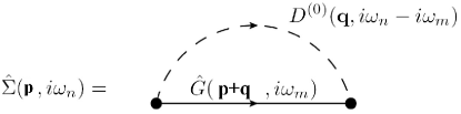
Figure 1: Second – order diagram for self – energy. Dashed line — phonon Green’s function $D^{(0)}$, continuous line — electron Green’s function $G$ in Matsubara representation.

In non – adiabatic case, when phonon energy becomes comparable with or even exceeds the Fermi energy, electron scattering is effective not only in the narrow energy layer around the Fermi surface, but in much wider energy interval of the order of $\Omega_{0}\sim E_{F}$. Then, for the case of initial $|{\bf p}|\sim p_{F}$ the averaging over ${\bf p^{\prime}}$ in expression like (3) should be done over the surface of constant energy, corresponding to $E_{F}+\Omega_{\bf p-p^{\prime}}$, as is shown in Fig. (2). Now the Eq. (3) is directly generalized as:

$$\noindent|g_{\bf pp^{\prime}}|^{2}\delta(\omega-\Omega_{\bf p-p^{\prime}})\Longrightarrow$$

$$\frac{1}{N(0)}\sum_{\bf p}\frac{1}{N(0)}\sum_{\bf p^{\prime}}|g_{\bf pp^{\prime}}|^{2}\times$$

$$\times\delta(\omega-\Omega_{\bf p-p^{\prime}})\delta(\varepsilon_{\bf p})\delta(\varepsilon_{\bf p^{\prime}}-\Omega_{\bf p-p^{\prime}})$$

$$\equiv\frac{1}{N(0)}\alpha^{2}(\omega)F(\omega)$$

(4)

After the replacement like (3) or (4) the explicit momentum dependence of the self – energy disappears and in fact in the following we are dealing with Fermi surface average of self – energy $\Sigma(\varepsilon)\equiv\frac{1}{N(0)}\sum_{\bf p}\delta(\varepsilon_{\bf p})\Sigma({\varepsilon,{\bf p}})$, which is now written as:

$$\Sigma(\varepsilon)=\int d\varepsilon^{\prime}\int d\omega\alpha^{2}(\omega)F(\omega)\Biggl{\{}\frac{f(\varepsilon^{\prime})}{\varepsilon-\varepsilon^{\prime}+\omega-i\delta}$$

$$+\frac{1-f(\varepsilon^{\prime})}{\varepsilon-\varepsilon^{\prime}-\omega+i\delta}\Biggr{\}}$$ (5)

This expression forms the basis of Eliashberg – McMillan theory and determines the structure of Eliashberg equations for the description of superconductivity.

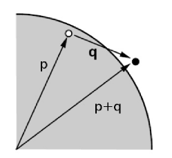
Figure 2: (a) Elementary act of electron – phonon scattering in the vicinity of the Fermi surface. (b) Surfaces of constant energy for initial and final states of an electron scattered by an optical phonon with energy comparable to Fermi energy. Non – trivial contribution to the average of the matrix element in (10) or (12) comes here from the intersection of these surfaces.

Now the self – energy is dependent only on frequency (and not on momentum) and we can use the following simple expressions, relating mass renormalization of an electron to the residue a the pole of the Green’s function Diagr :

$$Z^{-1}=1-\left.\frac{\partial\Sigma(\varepsilon)}{\partial\varepsilon}\right|_{\varepsilon=0}$$ (6)

$$m^{\star}=\frac{m}{Z}=m\left.\left(1-\frac{\partial\Sigma(\varepsilon)}{\partial\varepsilon}\right|_{\varepsilon=0}\right)$$ (7)

Then from Eq. (5) by direct calculations we obtain:

$$-\left.\frac{\partial\Sigma(\varepsilon)}{\partial\varepsilon}\right|_{\varepsilon=0}=2\int_{0}^{\infty}\frac{d\omega}{\omega}\alpha^{2}(\omega)F(\omega)\\$$

and introducing the dimensionless Eliashberg – McMillan electron – phonon coupling constant as:

$$\lambda=2\int_{0}^{\infty}\frac{d\omega}{\omega}\alpha^{2}(\omega)F(\omega)$$ (8)

we immediately obtain the standard expression for electron mass renormalization due to electron – phonon interaction:

$$m^{\star}=m(1+\lambda)$$ (9)

The function $\alpha^{2}(\omega)F(\omega)$ in the expression for Eliashberg – McMillan electron – phonon coupling constant (8) should be calculated according to (3) or (4) depending on the relation between Fermi energy $E_{F}$ and characteristic phonon frequency $\Omega_{0}$ As long as $\Omega_{0}\ll E_{F}$ we can use the standard expression (3), while in case of $\Omega_{0}\sim E_{F}$ we should use (4).

Using Eq. (4) we can rewrite (8) in the following form:

$$\lambda=\frac{2}{N(0)}\int\frac{d\omega}{\omega}\sum_{\bf p}\sum_{\bf p^{\prime}}|g_{\bf pp^{\prime}}|^{2}\times$$

$$\times\delta(\omega-\Omega_{\bf p-p^{\prime}})\delta(\varepsilon_{\bf p})\delta(\varepsilon_{\bf p^{\prime}}-\Omega_{\bf p-p^{\prime}})$$ (10)

which gives the most general expression to calculate the electron – phonon constant $\lambda$, determining pairing in Eliashberg – McMillan theory. Implicitly this result was contained already in Ref. Allen . Below we shall present some simple estimates, based on this general relation.

3 Estimates of electron – phonon coupling with non – adiabatic phonons

Let us consider the simplest possible model of electrons interacting with a single optical (Einstein – like) phonon mode with high – enough frequency $\Omega_{0}$. The general qualitative picture of such scattering is shown in Fig. 2. In this case in Eq. (10) the density of phonon states is simply $F(\omega)=\delta(\omega-\Omega_{0})$. Just for orientation we may take the possible momentum dependence of interaction with this optical phonon in the form proposed in Refs. FeSe_ARPES_Nature ; Dolg to describe nearly “forward” scattering by optical phonons at FeSe/STO interface, as a possible mechanism of strong $T_{c}$ enhancement in this system:

$$g({\bf q})=g_{0}\exp(-|{\bf q}|/q_{0}),$$ (11)

where the typical value of $q_{0}\ll p_{F}$ ($p_{F}$ is the Fermi momentum) to ensure the nearly “forward” nature of scattering. This model allows explicit estimates, which may illustrate the general situation.

Now we can write the dimensionless pairing constant of electron – phonon interaction in Eliashberg theory as:

$$\lambda=\frac{2}{N(0)\Omega_{0}}\sum_{\bf p}\sum_{\bf q}|g_{\bf q}|^{2}\delta(\varepsilon_{\bf p})\delta(\varepsilon_{\bf p+q}-\Omega_{0})$$ (12)

As in FeSe/STO with rather shallow conduction band FeSe_ARPES_Nature ; NPS_1 ; NPS_2 , where in fact we have $\Omega_{0}>E_{F}$, the finite value of $\Omega_{0}$ in the second $\delta$-function here should be definitely taken into account.

We can make our estimates assuming the simplest linearized form of electronic spectrum near the Fermi surface ($v_{F}$ is Fermi velocity): $\varepsilon_{\bf p}\approx v_{F}(|{\bf p}|-p_{F})$, which allows us to perform all calculations analytically. Using (11) in (12) and considering the two – dimensional case, after the calculation of all integrals we obtain NPS_2 :

$$\lambda=\frac{g_{0}^{2}a^{2}}{\pi^{2}v_{F}^{2}}K_{1}\left(\frac{2\Omega_{0}}{v_{F}q_{0}}\right),$$ (13)

where $K_{1}(x)$ is Bessel function of imaginary argument (McDonald function). Using the asymptotic form of $K_{1}(x)$ and dropping a number of irrelevant constants of the order of unity, we get:

$$\lambda\sim\lambda_{0}\frac{q_{0}}{4\pi p_{F}},$$ (14)

for $\frac{\Omega_{0}}{v_{F}q_{0}}\ll 1$, and

$$\lambda\sim\lambda_{0}\frac{\Omega_{0}}{\pi E_{F}}\sqrt{\frac{v_{F}q_{0}}{\Omega_{0}}}\exp\left(-\frac{2\Omega_{0}}{v_{F}q_{0}}\right),$$ (15)

for $\frac{\Omega_{0}}{v_{F}q_{0}}\gg 1$. Here we introduced the standard dimensionless electron – phonon coupling constant:

$$\lambda_{0}=\frac{2g_{0}^{2}}{\Omega_{0}}N(0),$$ (16)

where $N(0)$ is the density of electronic states at the Fermi level per single spin projection.

The result (14) is by itself rather unfavorable for significant $T_{c}$ enhancement in model under discussion, where $q_{0}\ll p_{F}$. Even worse is the situation if we take into account the large values of $\Omega_{0}$, as pairing constant becomes exponentially suppressed for $\frac{\Omega_{0}}{v_{F}q_{0}}>1$, which is typical for FeSe/STO interface, where $\Omega_{0}>E_{F}\gg v_{F}q_{0}$ UFN . This makes the enhancement of $T_{c}$ due to interaction of FeSe electrons with optical phonons of STO rather improbable, as was stressed in Ref. NPS_2 .

However, this is not our main point here. Actually, using (11) we can also make estimates for generally more typical case, when the optical phonon scatters electrons not only in nearly “forward” direction, but in a wider interval of transferred momenta. To do that we have simply to use in Eq. (11)the larger values of parameter $q_{0}$. Choosing e.g. $q_{0}\sim 4\pi p_{F}$ and using the low frequency limit of (14) we immediately obtain $\lambda\approx\lambda_{0}$, i.e. the standard result. Similarly, parameter $q_{0}$ can be taken of the order of inverse lattice vector $2\pi/a$ (where $a$ is the lattice constant). Then for $q_{0}\sim 2\pi/a$ from (14) we obtain:

$$\lambda\sim\lambda_{0}\frac{1}{2p_{F}a}\sim\lambda_{0}$$ (17)

for the typical case of $p_{F}\sim 1/2a$. In general there always remains the dependence on the value of Fermi momentum and cutoff parameter (cf. similar analysis in Ref. Diagr ). These particular estimates are valid for the adiabatic case.

In antiadiabatic limit of (15), assuming $q_{0}\sim p_{F}$ we immediately obtain:

$$\lambda\sim\frac{\sqrt{2}}{\pi}\lambda_{0}\sqrt{\frac{\Omega_{0}}{E_{F}}}\exp\left(-\frac{\Omega_{0}}{E_{F}}\right),$$ (18)

which simply signifies the effective interaction cutoff for $\Omega_{0}>E_{F}$ in the antiadiabatic limit. This fact was already noted by Gor’kov in Refs. Gork_1 ; Gork_2 , where it was stressed that in antiadiabatic limit the cutoff in the Cooper channel is determined not by the average phonon frequency, but by Fermi energy.

4 Antiadiabatic limit and mass renormalization

Our discussion up to now implicitly assumed the conduction band of an infinite width. However, it is obvious that in case of large enough characteristic phonon frequency it may become comparable with conduction band width, which in typical metal case is of the order of Fermi energy $E_{F}$. Now we will show that in the strongly nonadiabatic (antiadiabatic) limit, when $\Omega_{0}\gg E_{F}\sim D$ (here $D$ is the conduction band half-width), we are in fact dealing with the situation, when there appears a new small parameter of perturbation theory $\lambda D/\Omega_{0}\sim\lambda E_{F}/\Omega_{0}$.

Consider the case of conduction band of the finite width $2D$ with constant density of states (which formally corresponds to two – dimensional case). The Fermi level as always is considered as an origin of energy scale and for simplicity we assume the case of half – filled band. Then (5) reduces to:

$$\noindent\Sigma(\varepsilon)=\int_{-D}^{D}d\varepsilon^{\prime}\int d\omega\alpha^{2}(\omega)F(\omega)\Biggl{\{}\frac{f(\varepsilon^{\prime})}{\varepsilon-\varepsilon^{\prime}+\omega-i\delta}$$

$$+\frac{1-f(\varepsilon^{\prime})}{\varepsilon-\varepsilon^{\prime}-\omega+i\delta}\Biggr{\}}=$$

$$\noindent=\int d\omega\alpha^{2}(\omega)F(\omega)\Biggl{\{}\ln\frac{\varepsilon+D+\omega-i\delta}{\varepsilon-D-\omega+i\delta}$$

$$\noindent-\ln\frac{\varepsilon+\omega-i\delta}{\varepsilon-\omega+i\delta}\Biggr{\}}$$

For the model of a single optical phonon $F(\omega)=\delta(\omega-\Omega_{0})$ and we immediately obtain:

$$\Sigma(\varepsilon)=\alpha^{2}(\Omega_{0})F(\Omega_{0})\Biggl{\{}\ln\frac{\varepsilon+D+\Omega_{0}-i\delta}{\varepsilon-D-\Omega_{0}+i\delta}$$

$$\noindent-\ln\frac{\varepsilon+\Omega_{0}-i\delta}{\varepsilon-\Omega_{0}+i\delta}\biggr{\}}$$

(20)

Correspondingly, from (4) we get:

$$-\left.\frac{\partial\Sigma(\varepsilon)}{\partial\varepsilon}\right|_{\varepsilon=0}=2\int_{0}^{\infty}d\omega\alpha^{2}(\omega)F(\omega)\frac{D}{\omega(\omega+D)}\\$$

and we can define the new generalized coupling constant as:

$$\tilde{\lambda}=2\int_{0}^{\infty}\frac{d\omega}{\omega}\alpha^{2}(\omega)F(\omega)\frac{D}{\omega+D}$$ (21)

which for $D\to\infty$ reduces to the usual Eliashberg – McMillan constant (8), while for $D\to 0$ ($D\ll\Omega_{0}$) it gives the “antiadiabatic” coupling constant:

$$\lambda_{D}=2D\int\frac{d\omega}{\omega^{2}}\alpha^{2}(\omega)F(\omega)$$ (22)

Eq. (21) describes the smooth transition between the limits of wide and narrow conduction bands. Mass renormalization in general case is determined by $\tilde{\lambda}$:

$$m^{\star}=m(1+\tilde{\lambda})$$ (23)

For the model of a single optical phonon with frequency $\Omega_{0}$ we have:

$$\tilde{\lambda}=\frac{2}{\Omega_{0}}\alpha^{2}(\Omega_{0})\frac{D}{\Omega_{0}+D}=\lambda\frac{D}{\Omega_{0}+D}=\lambda_{D}\frac{\Omega_{0}}{\Omega_{0}+D}$$ (24)

where Eliashberg – McMillan constant is:

$$\lambda=2\int_{0}^{\infty}\frac{d\omega}{\omega}\alpha^{2}(\omega)F(\omega)=\alpha^{2}(\Omega_{0})\frac{2}{\Omega_{0}}$$ (25)

and $\lambda_{D}$ reduces to:

$$\lambda_{D}=2\alpha^{2}(\Omega_{0})\frac{D}{\Omega_{0}^{2}}=2\alpha^{2}(\Omega_{0})\frac{1}{\Omega_{0}}\frac{D}{\Omega_{0}}=\lambda\frac{D}{\Omega_{0}}$$ (26)

where in the last expression we explicitly introduced the new small parameter $D/\Omega_{0}\ll 1$, appearing in strong antiadiabatic limit. Correspondingly, in this limit we always have:

$$\lambda_{D}=\lambda\frac{D}{\Omega_{0}}\sim\lambda\frac{E_{F}}{\Omega_{0}}\ll\lambda$$ (27)

so that for reasonable values of $\lambda$ (even up to a strong coupling region of $\lambda\sim 1$) “antiadiabatic” coupling constant remains small. Obviously, all vertex corrections here are also small, as was shown rather long ago by direct calculations in Ref. Ikeda . Thus we come to an unexpected conclusion — in the limit of strong nonadiabaticity the electron – phonon coupling becomes weak and we obtain a kind of “anti – Migdal” theorem.

Physically, the weakness of electron – phonon coupling in strong nonadiabatic limit is more or less clear — when ions move much faster than electrons, these rapid oscillation are just averaged in time as electrons can not follow the very rapidly changing configuration of ions.

5 Eliashberg equations and the temperature of superconducting transition

All analysis above was performed for the normal state of a metal. Now let us turn to the superconducting phase. The problem arises, to what extent the results obtained can be generalized for the case of a metal in superconducting state? In particular, what coupling constant ($\lambda$ or $\tilde{\lambda}$) determines the temperature of superconducting transition $T_{c}$ in antiadiabatic limit? Let us analyze this situation within appropriate generalization of Eliashberg equations.

Taking into account that in antiadiabatic approximation vertex corrections are are again irrelevant and neglecting the direct Coulomb repulsion, Eliashberg equations can be derived in the usual way by calculating the diagram of Fig. 1, where electronic Green’s function in superconducting state is taken in Nambu’s matrix representation. For real frequencies this Green’s function is written in the following standard form Geb ; Izy :

$$G(\varepsilon,{\bf p})=\frac{Z(\varepsilon)\varepsilon\tau_{0}+\varepsilon_{\bf p}\tau_{3}+Z(\varepsilon)\Delta(\varepsilon)\tau_{1}}{Z^{2}(\varepsilon)\varepsilon^{2}-Z^{2}(\varepsilon)\Delta^{2}(\varepsilon)-\varepsilon^{2}_{\bf p}}$$ (28)

which corresponds to the matrix of self – energy:

$$\Sigma(\varepsilon)=[1-Z(\varepsilon)]\varepsilon\tau_{0}+Z(\varepsilon)\Delta(\varepsilon)\tau_{1}$$ (29)

where $\tau_{i}$ are standard Pauli matrices, while functions of mass renormalization $Z(\varepsilon)$ and energy gap $\Delta(\varepsilon)$ are determined from solution of integral Eliashberg equations Geb ; Izy . For us now it is sufficient to consider only the linearized Eliashberg equations, determining superconducting transition temperature $T_{c}$, which for the case of real frequencies are written as Geb ; Izy :

$$[1-Z(\varepsilon)]\varepsilon=\int_{0}^{D}d\varepsilon^{\prime}\int_{0}^{\infty}d\omega\alpha^{2}(\omega)F(\omega)f(-\varepsilon^{\prime})\times$$

$$\times\left(\frac{1}{\varepsilon^{\prime}+\varepsilon+\omega+i\delta}-\frac{1}{\varepsilon^{\prime}-\varepsilon+\omega-i\delta}\right)$$ (30)

$$Z(\varepsilon)\Delta(\varepsilon)=\int_{0}^{D}\frac{d\varepsilon^{\prime}}{\varepsilon^{\prime}}th\frac{\varepsilon^{\prime}}{2T_{c}}Re\Delta(\varepsilon^{\prime})\times$$

$$\times\int_{0}^{\infty}d\omega\alpha^{2}(\omega)F(\omega)\times$$

$$\times\left(\frac{1}{\varepsilon^{\prime}+\varepsilon+\omega+i\delta}+\frac{1}{\varepsilon^{\prime}-\varepsilon+\omega-i\delta}\right)$$ (31)

In difference with the standard approach Izy , we have introduced the finite integration limits, determined by the (half)bandwidth $D$. To simplify the analysis we again assume the half–filled band of degenerate electrons in two dimensions, so that $D=E_{F}\gg T_{c}$, with constant density of states.

Situation is considerably simplified Sad_1 ; Sad_2 , if we consider these equations in the limit of $\varepsilon\to 0$ and look for the solutions $Z(0)=Z$ and $\Delta(0)=\Delta$. Then from (30) we obtain:

$$[1-Z]\varepsilon=-2\varepsilon\int_{0}^{\infty}d\omega\alpha^{2}(\omega)F(\omega)\frac{D}{\omega(\omega+D)}$$ (32)

and we get the mass renormalization factor as:

$$Z=1+\tilde{\lambda}$$ (33)

where constant $\tilde{\lambda}$ was defined above in Eq. (21), which for $D\to\infty$ reduces to the usual Eliasberg – McMillan constant (8), while for $D$ significantly smaller than characteristic phonon frequencies it gives the “antiadiabatic” coupling constant (22). Mass renormalization is again determined by this generalized coupling constant $\tilde{\lambda}$ as in Eq. (23). In particular, in the strong antiadiabatic limit this renormalization is quite small and determined by the limiting expression $\lambda_{D}$ given by Eq. (22).

Situation is quite different in Eq. (31). In the limit of $\varepsilon\to 0$, using (33) we immediately obtain from (31) the following equation for $T_{c}$:

$$1+\tilde{\lambda}=2\int_{0}^{\infty}d\omega\alpha^{2}(\omega)F(\omega)\int_{0}^{D}\frac{d\varepsilon^{\prime}}{\varepsilon^{\prime}(\varepsilon^{\prime}+\omega)}th\frac{\varepsilon^{\prime}}{2T_{c}}$$ (34)

where $\lambda$ is the standard Eliashberg – McMillan coupling constant as defined above in Eq. (8). Thus, in general case, different coupling constants determine mass renormalization and $T_{c}$.

Let us consider rather general model with discrete set of dispersionless phonon modes (Einstein phonons). In this case the phonon density of states is written as:

$$F(\omega)=\sum_{i}\delta(\omega-\Omega_{i})$$ (35)

where $\Omega_{i}$ are discrete frequencies modeling the optical branches of the phonon spectrum. Then from Eqs. (8) and (21) we get:

$$\lambda=2\sum_{i}\frac{\alpha^{2}(\Omega_{i})}{\Omega_{i}}\equiv\sum_{i}\lambda_{i}$$ (36)

$$\tilde{\lambda}=2\sum_{i}\frac{\alpha^{2}(\Omega_{i})D}{\Omega_{i}(\Omega_{i}+D)}=\sum_{i}\lambda_{i}\frac{D}{\Omega_{i}+D}\equiv\sum_{i}\tilde{\lambda}_{i}$$ (37)

Correspondingly, in this case:

$$\alpha^{2}(\omega)F(\omega)=\sum_{i}\alpha^{2}(\Omega_{i})\delta(\omega-\Omega_{i})$$

$$=\sum_{i}\frac{\lambda_{i}}{2}\Omega_{i}\delta(\omega-\Omega_{i})$$ (38)

The standard Eliashberg equation (in adiabatic limit) for such model were consistently solved in Ref. KM . For our purposes it is sufficient to analyze only Eq. (34), which takes now the following form:

$$1+\tilde{\lambda}=2\sum_{i}\alpha^{2}(\Omega_{i})\int_{0}^{D}\frac{d\varepsilon^{\prime}}{\varepsilon^{\prime}(\varepsilon^{\prime}+\Omega_{i})}th\frac{\varepsilon^{\prime}}{2T_{c}}$$ (39)

This equation is easily solved to obtain:

$$T_{c}\sim\prod_{i}\left(\frac{D}{1+\frac{D}{\Omega_{i}}}\right)^{\frac{\lambda_{i}}{\lambda}}\exp\left(-\frac{1+\tilde{\lambda}}{\lambda}\right)$$ (40)

In the simple case of two optical phonons with frequencies $\Omega_{1}$ and $\Omega_{2}$ we have:

$$T_{c}\sim\left(\frac{D}{1+\frac{D}{\Omega_{1}}}\right)^{\frac{\lambda_{1}}{\lambda}}\left(\frac{D}{1+\frac{D}{\Omega_{2}}}\right)^{\frac{\lambda_{2}}{\lambda}}\exp\left(-\frac{1+\tilde{\lambda}}{\lambda}\right)$$ (41)

where $\tilde{\lambda}=\tilde{\lambda}_{1}+\tilde{\lambda}_{2}$ and $\lambda=\lambda_{1}+\lambda_{2}$. For the case of $\Omega_{1}\ll D$ (adiabatic phonon), and $\Omega_{2}\gg D$ (antiadiabatic phonon) Eq. (41) is immediately reduced to:

$$T_{c}\sim(\Omega_{1})^{\frac{\lambda_{1}}{\lambda}}(D)^{\frac{\lambda_{2}}{\lambda}}\exp\left(-\frac{1+\tilde{\lambda}}{\lambda}\right)$$ (42)

Now we can see, that in the preexponential factor the frequency of antiadiabatic phonon is replaced by band half–width (Fermi energy), which plays a role of the cutoff for logarithmic divergence in Cooper channel in antiadiabatic limit Sad_1 ; Gork_1 ; Gork_2 .

Our general result (40) gives the general expression for $T_{c}$ for the model with discrete set of optical phonons, valid both in adiabatic and antiadiabatic regimes and interpolating between these limits in intermediate region. Actually Eq. (40) can be easily rewritten as:

$$T_{c}\sim\langle\Omega\rangle\exp\left(-\frac{1+\tilde{\lambda}}{\lambda}\right)$$ (43)

where we have introduced the average logarithmic frequency $\langle\Omega\rangle$ as:

$$\ln\langle\Omega\rangle=\ln\prod_{i}\left(\frac{D}{1+\frac{D}{\Omega_{i}}}\right)^{\frac{\lambda_{i}}{\lambda}}=\sum_{i}\frac{\lambda_{i}}{\lambda}\ln\frac{D}{1+\frac{D}{\Omega_{i}}}$$ (44)

In the limit of continuous distribution of phonon frequencies this last expression reduces to:

$$\ln\langle\Omega\rangle=\frac{2}{\lambda}\int\frac{d\omega}{\omega}\alpha^{2}(\omega)F(\omega)\ln\frac{D}{1+\frac{D}{\omega}}$$ (45)

where $\lambda$ is given by the usual expression (8). Eq. (45) generalizes the standard definition of average logarithmic frequency of Eliasberg – McMillan theory Izy for the case of finite bandwidth. Obviously, it reduces to the standard expression in adiabatic limit of phonon frequencies much lower than $D$, and gives $\langle\Omega\rangle\sim D$ in extreme antiadiabatic limit, when all phonon frequencies are much larger than $D$.

6 Coulomb pseudopotential

Up to now we have neglected the direct Coulomb repulsion of electrons, which in the standard approach Schr ; Scal ; Geb ; Izy ; All is described by Coulomb pseudopotential $\mu^{\star}$, which is effectively suppressed by large Tolmachev’s logarithm. As we noted in Ref. Sad_1 antiadiabatic phonons actually suppress Tolmachev’s logarithm, which can probably lead to rather strong suppression of the temperature of superconducting transition. To clarify this situation we consider the simplified version of integral equation for the gap (31), writing it in the standard form:

$$Z(\varepsilon)\Delta(\varepsilon)=\int_{0}^{D}d\varepsilon^{\prime}K(\varepsilon,\varepsilon^{\prime})\frac{1}{\varepsilon^{\prime}}th\frac{\varepsilon^{\prime}}{2T_{c}}\Delta(\varepsilon^{\prime})$$ (46)

where the integral kernel is a combination of two step – functions:

$$K(\varepsilon,\varepsilon^{\prime})=\lambda\theta(\langle\Omega\rangle-|\varepsilon|)\theta(\langle\Omega\rangle-|\varepsilon^{\prime}|)$$

$$-\mu\theta(D-|\varepsilon|)\theta(D-|\varepsilon^{\prime}|)$$ (47)

where $\mu$ is the dimensionless (repulsive) Coulomb potential, while the parameter $\langle\Omega\rangle$, determining the energy width of attraction region due to phonons is determined by preexponential factor (average logarithmic frequency) of Eqs. (40),(43).

$$\langle\Omega\rangle=\prod_{i}\left(\frac{D}{1+\frac{D}{\Omega_{i}}}\right)^{\frac{\lambda_{i}}{\lambda}}$$ (48)

It is important that we always have $\langle\Omega\rangle<D$. Eq. (46) is now rewritten as:

$$Z(\varepsilon)\Delta(\varepsilon)=(\lambda-\mu)\int_{0}^{\langle\Omega\rangle}\frac{d\varepsilon^{\prime}}{\varepsilon^{\prime}}th\frac{\varepsilon^{\prime}}{2T_{c}}\Delta(\varepsilon^{\prime})$$

$$-\mu\int_{\langle\Omega\rangle}^{D}\frac{d\varepsilon^{\prime}}{\varepsilon^{\prime}}\Delta(\varepsilon^{\prime})$$ (49)

Writing the mass renormalization due to phonons as:

$$Z(\varepsilon)=\left\{\begin{array}[]{c}1+\tilde{\lambda}\quad\mbox{for}\quad\varepsilon<\langle\Omega\rangle\\ 1\quad\mbox{for}\quad\varepsilon>\langle\Omega\rangle\end{array}\right.$$ (50)

we look for the solution of Eq. (46) for $\Delta(\varepsilon)$, as usual, in the following form Scal ; Izy ; All :

$$\Delta(\varepsilon)=\left\{\begin{array}[]{c}\Delta_{1}\quad\mbox{for}\quad\varepsilon<\langle\Omega\rangle\\ \Delta_{2}\quad\mbox{for}\quad\varepsilon>\langle\Omega\rangle\end{array}\right.$$ (51)

Then Eq. (49) is transformed into the system of two homogeneous linear equations for constants $\Delta_{1}$ and $\Delta_{2}$:

$$(1+\tilde{\lambda})\Delta_{1}=(\lambda-\mu)\ln\frac{\langle\Omega\rangle}{T_{c}}\Delta_{1}-\mu\ln\frac{D}{\langle\Omega\rangle}\Delta_{2}$$

$$\Delta_{2}=-\mu\ln\frac{\langle\Omega\rangle}{T_{c}}\Delta_{1}-\mu\ln\frac{D}{\langle\Omega\rangle}\Delta_{2}$$ (52)

The condition of the existence of nontrivial solution here is:

$$1+\tilde{\lambda}=\left(\lambda-\frac{\mu}{1+\mu\ln\frac{D}{\langle\Omega\rangle}}\right)\ln\frac{\langle\Omega\rangle}{T_{c}}$$ (53)

Then the transition temperature is given by:

$$T_{c}=\langle\Omega\rangle\exp\left(-\frac{1+\tilde{\lambda}}{\lambda-\mu^{\star}}\right)$$ (54)

where the Coulomb pseudopotential is determined as:

$$\mu^{\star}=\frac{\mu}{1+\mu\ln\frac{D}{\langle\Omega\rangle}}=\frac{\mu}{1+\mu\ln\prod_{i}\left(1+\frac{D}{\Omega_{i}}\right)^{\frac{\lambda_{i}}{\lambda}}}$$ (55)

Now the phonon frequencies enter Tolmachev’s logarithm as the product of partial contributions, with its values determined also by corresponding coupling constants. Similar structure of Tolmachev’s logarithm was first obtained (in somehow different model) in Ref. KMK , where the case of frequencies going outside the limits of adiabatic approximation was not considered. In this sense, Eq. (55) has a wider region of applicability. In particular, for the model of two optical phonons with frequencies $\Omega_{1}\ll D$ (adiabatic phonon) and $\Omega_{2}\gg D$, from Eq. (55) we get:

$$\mu^{\star}=\frac{\mu}{1+\mu\ln\left(\frac{D}{\Omega_{1}}\right)^{\frac{\lambda_{1}}{\lambda}}}=\frac{\mu}{1+\mu\frac{\lambda_{1}}{\lambda}\ln\frac{D}{\Omega_{1}}}$$ (56)

We can see, that the contribution of antiadiabatic phonon drops out of Tolmachev’s logarithm, while the logarithm itself persists, with its value determined by the ratio of the band halfwidth (Fermi energy) to the frequency of adiabatic (low frequency) phonon. The general effect of suppression of Coulomb repulsion also persists, though it becomes somehow weaker due to the partial interaction of electrons with corresponding phonon. This situation is conserved also in the general case — the value of Tolmachev’s logarithm and corresponding Coulomb pseudopotential is determined by contributions of adiabatic phonons, while antiadiabatic phonons drop out. Thus, in general case, situation becomes more favorable for superconductivity, as compared to the case of a single antiadiabatic phonon, considered in Ref. Sad_1 .

7 Conclusions

In present paper we have considered the electron – phonon coupling in Eliashberg – McMillan theory, taking into account antiadiabatic phonons with high enough frequency (comparable or exceeding the Fermi energy $E_{F}$). The value of mass renormalization, in general case, was shown to be determined by the new coupling constant $\tilde{\lambda}$, while the value of the pairing interaction is always determined by the standard coupling constant $\lambda$ of Eliashberg – McMillan theory, appropriately generalized by taking into account the finite value of phonon frequency Sad_1 . Mass renormalization due to strongly antiadiabatic phonons is in general small and determined by the coupling constant $\lambda_{D}\ll\lambda$. In this sense, in the limit of strong antiadiabaticity, the coupling of such phonons with electrons becomes weak and corresponding vertex correction again become irrelevant Ikeda ; Sad_1 , creating a kind of “anti – Migdal” situation. This fact allows us to use Eliashberg – McMillan approach in the limit of strong antiadiabaticity. In the intermediate region all our expressions just produce a smooth interpolation between adiabatic and antiadiabatic limits.

The cutoff of pairing interaction in Cooper channel in antiadiabatic limit becomes effective at energies $\sim E_{F}\sim D$, as was previously noted in Refs. Gork_1 ; Gork_2 ; Sad_1 ), so that corresponding phonons do not contribute to Tolmachev’s logarithm in Coulomb pseudopotential. However, the large enough values of this logarithm (and corresponding smallness of $\mu^{\star}$) can be guaranteed due to contributions from adiabatic phonons Sad_2 .

Note that above we have used rather simplified analysis of Eliashberg equations. However, in our opinion, more elaborate approach, e.g. along the lines of Ref. KM , will not lead to qualitative change of our results. Some simple estimates for FeSe/STO system, based on these results, can be found in Refs. Sad_1 ; Sad_2 .

- (1) J.R. Schrieffer. Theory of Superconductivity, WA Benjamin, NY, 1964
- (2) D.J. Scalapino. In “Superconductivity”, p. 449, Ed. by R.D. Parks, Marcel Dekker, NY, 1969
- (3) R.M. White, T.H. Geballe. Long Range Order in Solids. Academic Press, New York, San Francisco, London, 1979
- (4) S.V. Vonsovsky, Yu.A. Izyumov, E.Z. Kurmaev. Superconductivity of Transition metals, Their Alloys and Compounds, Springer, Berlin – Heidelberg, 1982
- (5) P.B. Allen, B. Mitrović. Solid State Physics, Vol. Vol. 37 (Eds. F. Seitz, D. Turnbull, H. Ehrenreich), Academic Press, NY, 1982, p. 1
- (6) A.B. Migdal. Zh. Eksp. Teor. Fiz. 34, 1438 (1958) [Sov. Phys. JETP 7, 996 (1958)]
- (7) A.S. Alexandrov. A.B. Krebs. Usp. Fiz. Nauk 162, 1 (1992) [Physics Uspekhi 35, 345 (1992)]
- (8) I. Esterlis, B. Nosarzewski, E.W. Huang, D. Moritz, T.P. Devereux, D.J. Scalapino, S.A. Kivelson. Phys. Rev. B 97, 140501(R) (2018)
- (9) M.V. Sadovskii. Usp. Fiz. Nauk 178, 1243 (2008) [Physics Uspekhi 51, 1243 (2008)]
- (10) L.P. Gor’kov, V.Z. Kresin. Rev. Mod. Phys. 90, 011001 (2018)
- (11) L.P. Gor’kov. PNAS 113, 4646 (2018)
- (12) L.P. Gor’kov. Phys. Rev. B93, 054517 (2016)
- (13) L.P. Gor’kov. Phys. Rev. B93, 060507 (2016)
- (14) M.V. Sadovskii.Zh. Eksp. Teor. Fiz 155, 527 (2019) [JETP 128, 455 (2019)]
- (15) M.V. Sadovskii. Pis’ma Zh. Eksp. Teor. Fiz. 109, 165 (2010) [JETP Letters 109, 166 (2019)]
- (16) M.V. Sadovskii. Diagrammatics. World Scientific, Singapore, 2006
- (17) P.B. Allen. Phys. Rev. B 6, 2577 (1972)
- (18) J.J. Lee, F.T. Schmitt, R.G. Moore, S. Johnston, Y.T. Cui,W. Li, Z.K. Liu, M. Hashimoto, Y. Zhang, D.H. Lu, T.P. Devereaux, D.H. Lee, Z.X. Shen. Nature 515, 245 (2014)
- (19) M.L. Kulić, O.V. Dolgov. New J. Phys. 19, 013020 (2017)
- (20) I.A. Nekrasov, N.S. Pavlov, V.V. Sadovskii. Pis’ma Zh. Eksp. Teor. Fiz. 105, 354 (2017) [JETP Letters 105, 370 (2017)]
- (21) I.A. Nekrasov, N.S. Pavlov, M.V. Sadovskii. Zh. Eksp. Teor. Fiz. 153, 590 (2018) [JETP 126, 485 (2018)] Phys. Rev. B 93, 134513 (2016)
- (22) M.A. Ikeda, A. Ogasawara, M. Sugihara. Phys. Lett. A 170, 319 (1992)
- (23) A.E. Karakozov, E.G. Maksimov, S.A. Mashkov. Zh. Eksp. Teor. Fiz. 68, 1937 (1975) [JETP 41, 971 (1975)]
- (24) D.A. Kirzhnits, E.G. Maksimov, D.I. Khomskii. J. Low. Temp. Phys. 10, 79 (1973)