Efficiency Fairness Tradeoff in Battery Sharing

Abstract

The increasing presence of decentralized renewable generation in the power grid has motivated consumers to install batteries to save excess energy for future use. The high price of energy storage calls for a shared storage system, but careful battery management is required so that the battery is operated in a manner that is fair to all and as efficiently as possible. In this paper, we study the tradeoffs between efficiency and fairness in operating a shared battery. We develop a framework based on constrained Markov decision processes to study both regimes, namely, optimizing efficiency under a hard fairness constraint and optimizing fairness under hard efficiency constraint. Our results show that there are fundamental limits to efficiency under fairness and vice-versa, and, in general, the two cannot be achieved simultaneously. We characterize these fundamental limits via absolute bounds on these quantities, and via the notion of price of fairness that we introduce in this paper.

I Introduction

The falling cost of solar panels and incentives for renewable generation has created hope for massively decentralized power generation. Islanded microgrids can install wind generators, individual households, housing societies, and industries can generate their own energy via solar panels, and reduce both, their reliance on the grid and their carbon footprint. However, unpredictability and unreliability of renewable energy also necessitate battery backup to store excess energy, so that it can be utilized at times when this generation is low. With adequate battery backup, one can envision a future where there is widespread deployment of renewable generation, leading to a higher penetration of clean energy sources. A key component in realizing this dream is the cost of the battery. While solar panels have become inexpensive in the recent past, batteries prices continue to be stiff and significant.

The high cost of battery storage has motivated communities to look for sharing contracts that provide users access to a common battery, leading to sharing of the overall costs. The shared battery is expected to serve as collective storage accessible by multiple users that can be utilized to store excess generation, which users may want to withdraw at times of deficit. However, like anyone who has used a shared refrigerator at a dorm would realize, sharing of a storage space brings with it concerns about the inequity of access and the possibility of other users ‘stealing’ one’s content. Clearly, gate-keeping is required so that users access the battery in a manner that is fair to all, and yet the battery is operated in an efficient manner that fully exploits the investment made in installing it. We are motivated by this question of fair and efficient operation of a shared battery.

For the success of the sharing arrangement, it should ideally allow each user to access the common battery as if it is wholly owned by the user without jeopardizing the access of other users. But if users have disparate generation characteristics, excessive charging by one user may leave another user with less opportunity to deposit his energy, diminishing equity of access. At the other extreme, it is evident that without a formal algorithm to do the gate-keeping, some users could draw far more energy than they injected, thereby cannibalizing the energy of other users.

Moreover, it seems plausible that gate-keeping may compel the battery operator to decline requests for injection even while there is room in the battery, or for withdrawal of energy even there is energy in the battery. As a consequence, maintaining fairness may come in the way of efficient battery operation. In this paper, we develop a framework to quantify the tradeoffs between efficiency and fairness in the operation of a shared battery. Our work shows that there is a precise sense in which the requirement of fairness fundamentally compromises efficiency, and in general, the two cannot be achieved simultaneously. We also quantify the tradeoff by characterizing the maximum efficiency achievable under fairness, and the maximum fairness achievable under efficiency.

We consider a setting where $N$ users with individual stochastic net generation access a shared battery. The net generation may be positive (in which case the user wishes to inject energy) or negative (draw energy). We posit that a battery management algorithm decides the amount of energy to accept from injecting users and to provide to demanding users. We adopt a general principle of fairness that no user should draw more energy from the battery than it has injected into it. However, since energy units added by users are fungible, in the sense that they are indistinguishable from those added by other users, the above principle need not be applied sequentially. The battery management algorithm can allow users an ‘overdraft’, where users can for some intervals, draw more energy from the battery than they have injected thus far, so long as the energy is ‘returned’ at a later stage. Specifically, in our notion of fairness, we ask that for each user, the long-run time average of the energy drawn from the battery by the user be no more than the long-run time average of the energy injected. Our notion of efficiency is the loss of load rate (LLR). The LLR of user $i$ is its long run time average of unmet demand.

We first study the problem of maximizing the efficiency subject to hard constraints on fairness and derive fundamental limits on the minimum total LLR attainable under fairness constraints. We show that when there is at least one user that is net demanding, i.e., has negative steady-state net generation on average; the total LLR remains bounded away from zero for any battery size. Remarkably, this is true even when the total steady-state average net generation of all users is positive. In contrast, in the absence of the fairness constraint, the total LLR, in this case, would decrease exponentially with battery size. When all users are net generative (i.e., with positive steady state net generation on average), the LLR even with the fairness constraint decreases to zero exponentially with the battery size.

Given that the fairness constraint limits the efficient use of the battery, we then ask the price of fairness. This is defined as the ratio of the minimum attainable total LLR with the fairness constraint, to that attained without the fairness constraint. Our fundamental limits already show that this ratio approaches infinity for large battery size when at least one user is net demanding, but the system is net generative on the whole. However, remarkably, we show that the price of fairness can be arbitrarily large even all users are net generative.

Finally, we study the maximum fairness attainable under efficient battery use. We find numerically that efficient battery operation often compromises fairness for at least one user. Moreover, that departure from the utopian fairness persists even when one increases the battery size. This shows that the conflict between efficiency and fairness is, in a sense, fundamental and that a larger battery does not remedy it. These results provide a natural motivation for devising a market for energy wherein a user can inject its excess energy into the battery, which can then be sold to other users. The precise formulation for such a market is a point for future study.

Literature Survey

There is recent literature on the effects of energy/battery sharing in power systems. The effects of sharing energy are studied from a (non-cooperative) game-theoretic perspective in [2]. The strategic decision is to choose the investment in individual battery storage systems. On the other hand, [3] views this problem from a coalition game perspective. Investment in a shared battery and the corresponding allocation scheme is studied in [4]. All these models assume the net generation observed by the battery to be independent and identically distributed random variables (i.i.d.) across time. This seriously limits the applicability of the system as the net generation is generally dependent across time. In contrast, we consider Markov models for net generation, which can better model the behaviour of renewable energy sources.

Markov energy generation models for scheduling of energy storage have been considered in [5], [6]. [5] models the system as a finite-horizon Markov decision process (MDP) where the decision of buying or selling electricity is made by an operator. They provide threshold based heuristic policies and quantify their suboptimality. [7] studies the problem of scheduling and operation of energy storage for wind power plants. [8] considers an infinite horizon discounted MDP based model to determine the optimal amount of battery to be bought from the grid to minimize the cost given a battery of fixed capacity. These papers focus on providing structural results of optimal policies and/or heuristic algorithms. On the other hand, we consider a model in which we minimize the expected loss of load if all demand is to be satisfied by only the renewable generation and the common battery. Our main distinction is the introduction of a notion of fairness, which, to the best of our knowledge, has not been done before in the scheduling of energy storage. Using this notion, we study the tradeoff between efficiency and fairness in the operation of shared energy storage systems.

II Model and Preliminaries

II-A Notation

In general, we denote random variables by capital letters and the value taken by a random variable is denoted by the corresponding lower case letters. $\prod_{i\in I}V_{i}$ denotes the Cartesian product of sets $V_{i},\ i\in I$. $\{u,\ldots,v\}$ is the set of integers from $u$ to $v$. $[n]$ denotes the set $\{1,\ldots,n\}$.

II-B Model

Consider $n$ users $\{1,\ldots,n\}$ equipped with stochastic net generation evolving in discrete time. The net energy generation of user $i$ at time $t$ be denoted by $X_{i}(t)\in S_{i}.$ A positive value of $X_{i}(t)$ indicates a net surplus at time $t$ (i.e., user $i$ generated more energy than she consumed) whereas a negative value of $X_{i}(t)$ indicates a net deficit at time $t$ (i.e., user $i$ demanded more energy than she generated). We assume an arbitrary positive granularity with which energy generation/demand is measured; this granularity is taken to be unity without loss of generality, so that $S_{i}\subset{\mathbb{Z}}.$ Let $s^{+}_{i}$ denote the maximum energy user $i$ injects and $-s^{-}_{i}$ denote the maximum energy user $i$ demands, i.e., $s^{+}_{i}=\max_{s\in S_{i}}s$ and $s^{-}_{i}=\min_{s\in S_{i}}s$. To avoid degenerate scenarios, we assume that $s^{+}_{i}>0$ and $s^{-}_{i}<0.$

Let $X(t)=\{X_{1}(t),\ldots,X_{n}(t)\}$. We assume that $X(\cdot)$ is an irreducible discrete time Markov chain (DTMC) over a finite state space $S\subseteq\prod_{i\in[n]}S_{i}.$ Note that we do not assume here that the net generation processes associated with the individual users are independent. We make the assumption that $\mathbb{P}\left[X(t+1)=s\ |\ X(t)=s\right]>0$ for all $s\in S.$ Note that this ensures aperiodicity of $X(\cdot).$

Let $\pi=(\pi(s),s\in S)$ denote the stationary distribution of the DTMC $X(\cdot).$ We define the drift $\Delta_{i}$ associated with user $i$ as her steady state average net generation:

$$\Delta_{i}=\sum_{s\in S}s_{i}\pi(s),$$

where $s=(s_{1},\ldots,s_{n}).$ User $i$ is said to be net generative if $\Delta_{i}>0$ and net demanding if $\Delta_{i}<0.$ The system drift $\Delta$ is defined the sum of the user drifts, i.e., $\Delta=\sum_{i\in[n]}\Delta_{i}.$

A common battery with capacity $b_{\max}\in{\mathbb{N}}$ is shared between the users. The battery occupancy at time $t$ is a random variable denoted by $B(t)$. $(X(t),B(t))$ is a controlled Markov process evolving over

$${\bf S}=S\times[b_{\max}].$$ (1)

Battery dynamics are given by

$$B(t+1)=B(t)+\sum_{i\in[n]}A_{i}(t),$$ (2)

where $A_{i}(t)$ denotes the energy accepted from user $i$ (when $A_{i}(t)\geq 0$) or the energy supplied to user $i$ (when $A_{i}(t)<0$). We assume that the actions $A_{i}(t),i\in[n]$ at each time instant $t$ are chosen by the battery operator as a function of the state history $(X(s),B(s)),$ $s\leq t$.

The battery management algorithm is constrained as follows. In state $(x,b)\in{\bf S}$, the space of allowable actions, denoted by $A(x,b),$ is given by:

$$A(x,b) =\biggl{\{}(a_{1},\ldots,a_{n})\ |\ a_{i}\in\begin{cases}\{0,\ldots,x_{i}\},&{\rm if}\ x_{i}\geq 0\\ \{x_{i},\ldots,0\},&{\rm if}\ x_{i}<0\end{cases},$$

$$\quad\quad 0\leq b+\sum_{i\in[n]}a_{i}\leq b_{\max}\biggr{\}}$$ (3)

$${\bf A} =\bigcup_{(x,b)\in{\bf S}}A(x,b)$$

The above constraints restrict the amount of energy supplied to a user by the amount demanded and similarly restricts the amount of energy accepted from a user by her net surplus. In addition, the actions must also respect the capacity constraints of the battery, and that the battery cannot be discharged below 0.

II-C Loss of Load Rate (LLR)

Our notion of efficiency is defined by the loss of load rate. The loss of load rate (${\rm LLR}$) for user $i,$ denoted by ${\rm LLR}_{i},$ is defined as:

$${\rm LLR}_{i}\coloneqq\lim_{T\rightarrow\infty}\frac{1}{T}\sum_{t=0}^{T}\mathbb{E}[\mathbb{I}\{X_{i}(t)<0\}(A_{i}(t)-X_{i}(t))]$$ (4)

Note that ${\rm LLR}_{i}\geq 0,$ since $A_{i}(t)\geq X_{i}(t)$ when $X_{i}(t)<0$ from section II-B. ${\rm LLR}_{i}$ captures the long run average rate of unmet demand for user $i.$ For a system of $n$ users, we define the ${\rm LLR}$ of the system to be the sum of ${\rm LLR}$s of the individual users, i.e., ${\rm LLR}_{\rm sys}=\sum_{i\in[n]}{\rm LLR}_{i}$.

III Maximizing Efficiency with Hard Constraints on Fairness

In this section, we study the tradeoff between efficiency and fairness by putting a hard constraint on fairness and optimizing efficiency under this constraint. The notion of fairness we consider is that for each user, the time-averaged amount of energy drawn from the battery is at most the time-averaged amount of energy injected into the battery by that user. Efficiency is measured using the LLR. We formulate this problem as a constrained Markov decision process, and based on this formulation, derive fundamental limits on the efficiency achievable under fairness constraints.

III-A Constrainted Markov decision process formulation

In this section, we impose a set of service constraints that the battery management algorithm must satisfy, in order to impart fairness in battery scheduling.

$${\rm FC}_{i}:\qquad\lim_{T\rightarrow\infty}\frac{1}{T}\sum_{t=0}^{T}\mathbb{E}[A_{i}(t)]{\geq}0.$$ (5)

${\rm FC}_{i}$ asks that the amount of energy we provide to each user is at most the amount of energy the user injects into the battery. We call $\lim_{T\rightarrow\infty}\frac{1}{T}\sum_{t=0}^{T}\mathbb{E}[A_{i}(t)]$ the net contribution (C_i) of source $i$. We impose that the battery management algorithm satisfy ${\rm FC}_{i}$ for all $i\in[n]$, collectively referred to as fairness constraints.

We consider the problem of operating the system under fairness constraints so that ${\rm LLR}_{\rm sys}$ is minimized. This problem is an instance of a constrained Markov decision process (we refer the reader to [9] for a survey), or CMDP with the average cost criterion. The state space is given by 1, and the set of allowable actions for each state is given by section II-B. The problem, for a fixed initial distribution on the state space, is summarized below:

(P) $\displaystyle\mathop{\hbox{\rm minimize}}_{\phi}$ $\underset{{T\rightarrow\infty}}{\lim}\frac{1}{T}\underset{t=0}{\overset{T}{\sum}}\underset{{i\in[N]}}{\sum}\mathbb{E}[\mathbb{I}\{X_{i}(t)<0\}(A_{i}(t)-X_{i}(t))]$ subject to $\underset{T\rightarrow\infty}{\lim}\frac{1}{T}\underset{t=0}{\overset{T}{\sum}}\mathbb{E}[A_{i}(t)]{\geq}0\qquad\forall i\in[n].$

Here the decision variable is $\phi$, a randomized, history-dependent policy. A randomized policy is a sequence of functions $\phi(t),t\in{\mathbb{N}}$ that map the set of histories until time $t$ to probability distributions on the set of available actions at time $t$. The set of available actions in state $(x,b)\in{\bf S}$ is given by (II-B). A deterministic policy maps the set of histories to a specific available action at each time $t\in{\mathbb{N}}.$ A policy is Markov if it depends only on current state $(X(t),b(t))$ and it is stationary if $\phi(t)$ does not depend on $t$.

The CMDP (P) is tractable since it can be solved by solving an equivalent linear problem (LP) (see [9, 10]); we do not provide the details of this reduction here due to space constraints, though we do present the LP reduction for the CMDP posed in Section V for optimization of fairness given a hard constraint on efficiency. Note also that the CMDP (P) is defined for a given initial distribution on ${\bf S}$; as such its optimal value depends on this initial distribution. However, the choice of this initial distribution does not affect the results we derive in this paper.

III-B Fundamental limits

Denote the set of net demanding and net generating sources by

$$\mathscr{D}:=\{i\in[n]|\Delta_{i}<0\},\quad\mathscr{G}:=\{i\in[n]|\Delta_{i}>0\}.$$

The following theorem provides a lower bound on the objective of (P) under any policy.

Theorem III.1

$${\rm LLR}_{\rm sys}\geq\sum_{i\in\mathscr{D}}(-\Delta_{i}).$$

Proof:

It suffices to prove the stated lower bound on ${\rm LLR}_{\rm sys}$ under any feasible policy for (P).

$${\rm LLR}_{i} =\lim_{T\rightarrow\infty}\frac{1}{T}\sum_{t=0}^{T}\mathbb{E}[\mathbb{I}\{X_{i}(t)<0\}(A_{i}(t)-X_{i}(t))]$$

$$=\lim_{T\rightarrow\infty}\frac{1}{T}\sum_{t=0}^{T}\mathbb{E}[\mathbb{I}\{X_{i}(t)<0\}A_{i}(t)]$$

$$\quad+\lim_{T\rightarrow\infty}\frac{1}{T}\sum_{t=0}^{T}\mathbb{E}[\mathbb{I}\{X_{i}(t)>0\}X_{i}(t)]-\lim_{T\rightarrow\infty}\frac{1}{T}\sum_{t=0}^{T}\mathbb{E}[X_{i}(t)]$$

$$\stackrel{{\scriptstyle(a)}}{{\geq}}\lim_{T\rightarrow\infty}\frac{1}{T}\sum_{t=0}^{T}\mathbb{E}[\mathbb{I}\{X_{i}(t)<0\}A_{i}(t)]$$

$$\quad+\lim_{T\rightarrow\infty}\frac{1}{T}\sum_{t=0}^{T}\mathbb{E}[\mathbb{I}\{X_{i}(t)>0\}A_{i}(t)]-\lim_{T\rightarrow\infty}\frac{1}{T}\sum_{t=0}^{T}\mathbb{E}[X_{i}(t)]$$

$$=\lim_{T\rightarrow\infty}\frac{1}{T}\sum_{t=0}^{T}\mathbb{E}[A_{i}(t)]-\lim_{T\rightarrow\infty}\frac{1}{T}\sum_{t=0}^{T}\mathbb{E}[X_{i}(t)]$$

$$\stackrel{{\scriptstyle(b)}}{{\geq}}-\lim_{T\rightarrow\infty}\frac{1}{T}\sum_{t=0}^{T}\mathbb{E}[X_{i}(t)]=-\Delta_{i}$$

The inequality $(a)$ follows since $A_{i}(t)\leq X_{i}(t)$ when $X_{i}(t)>0.$ The inequality $(b)$ is a consequence of our fairness constraint. The statement of the lemma now follows by summing over all net demanding sources.  

The above bound shows that ${\rm LLR}_{\rm sys}$ remains bounded away from zero when $\mathscr{D}\neq\emptyset$ for any battery size. We next consider the case when all sources are net generative, i.e., $\mathscr{G}=[n]$. We show that in this case the optimal ${\rm LLR}_{\rm sys}$ goes down to zero exponentially with increasing battery size. To show this, we upper bound the optimal ${\rm LLR}_{\rm sys}$ by an expression which exponentially decays to 0. For this, we extensively use Theorem A.1 from Appendix A. It shows that the optimal LLR for a single net generating user decays exponentially in battery size. Using this, we now show that the exponential decay of the optimal LLR is true even for multiple sources, if all of them are net generating.

Theorem III.2

If $\mathscr{G}=[n]$, we have

$$\underset{b_{\max}\rightarrow\infty}{\lim{\rm sup}}\frac{\log({\rm LLR}_{o})}{b_{\max}}=-c,$$

where ${\rm LLR}_{o}$ denotes the optimal ${\rm LLR}$, $b_{\max}$ is the battery size and $c$ is a positive constant.

Proof:

We upper bound the solution of (P) by considering a particular policy. We divide the battery into $n$ equal chunks of size $\frac{b_{\max}}{n},$ allocating one chunk to each user. Consider the policy that optimally schedules each user using only the battery chunk allocated to her; as we mention in Appendix A, simple greedy operation is optimal when a battery (chunk) is used by used by a single user. Moreover, it is easy to see that this policy is fair.

Under the above policy, let ${\rm LLR}_{i}$ denote the loss of load rate of source $i$. Then, the ${\rm LLR}_{\rm sys}$ of the combined system under this policy is $\sum_{i=1}^{n}{\rm LLR}_{i}$. We know from Theorem A.1 that

$$\lim_{b_{\max}\rightarrow\infty}\frac{\log({\rm LLR}_{i})}{b_{\max}}=-c_{i},$$ (6)

for some positive constant $c_{i}$. Without loss of generality, let $c_{1}\leq c_{2}\leq\ldots\leq c_{n}$. It is not hard to see now that

$$\underset{b_{\max}\rightarrow\infty}{\lim{\rm sup}}\frac{\log({\rm LLR}_{\rm sys})}{b_{\max}}=-c_{1},$$

which implies the statement of the theorem.  

IV Price of Fairness

In this section, we analyse the efficiency implications of the fairness constraint (5) in the LLR optimization formulation (P) introduced in the previous section. We introduce the notion of Price of Fairness (PoF), which is the ratio of the optimal LLR subject to the fairness constraint, to the optimal LLR without this constraint. The main conclusion of this section is that the PoF can be arbitrarily large, even when all users are net generative. This means that imposing a strong fairness constraint in battery sharing can result in a substantial loss of efficiency. In the following section, we address this issue by proposing an alternative formulation that seeks to maximize fairness subject to maximal efficiency.

To define PoF, let ${\rm LLR}_{e}$ denote the optimal loss of load rate without the fairness constraint, i.e.,

$${\rm LLR}_{e}\coloneqq\min_{\phi}\lim_{T\rightarrow\infty}\frac{1}{T}\sum_{t=0}^{T}\sum_{i=1}^{n}\mathbb{E}[\mathbb{I}\{X_{i}(t)<0\}(A_{i}(t)-X_{i}(t))].$$

We refer to policies that solve the above optimization as efficient policies. It is not hard to see that the optimal loss of load rate is achieved by any greedy policy that (i) always charges the battery whenever energy is available, and (ii) always meets user demand whenever feasible. Formally, any policy that chooses actions that satisfy the following conditions is efficient.

1. If $0\leq b+\sum_{i\in[n]}x_{i}\leq b_{\max},$ then $a=x.$

2. If $b+\sum_{i\in[n]}x_{i}>b_{\max},$ then $a_{i}=x_{i}$ for all $i$ satisfying $x_{i}<0,$ and $b+\sum_{i\in[n]}a_{i}=b_{\max}.$

3. If $b+\sum_{i\in[n]}x_{i}<0,$ then $a_{i}=x_{i}$ for all $i$ satisfying $x_{i}>0,$ and $b+\sum_{i\in[n]}a_{i}=0.$

Let the space of actions $(a_{1},\ldots,a_{n})$ that satisfy the above efficiency conditions in state $(x,b)$ be denoted by $A_{e}(x,b)$ and the history dependent policies that satisfy these action constraints be denoted by $\Phi_{e}.$

The price of fairness (PoF) is defined as

$${\rm PoF}=\frac{{\rm LLR}_{o}}{{\rm LLR}_{e}}.$$ (7)

To analyse the PoF, we first consider the case where there is at least one net demanding source. In this case, if the system drift is itself negative, it is easy to see that ${\rm LLR}_{o}$ is bounded away from zero (using the same argument as in the proof of Theorem III.1). Thus, the more interesting case is $\Delta>0.$ In this case, the following lemma shows that the PoF grows to infinity as $b_{\max}\rightarrow\infty.$

Lemma IV.1

Suppose that $|\mathscr{D}|\geq 1$ (i.e., $\Delta_{i}<0$ for some $i$) but the system is net generative (i.e., $\Delta>0$). Then PoF $\rightarrow\infty$ as $b_{\max}\rightarrow\infty.$

Proof:

By Theorem III.1, ${\rm LLR}_{o}$ is bounded away from zero for any value of $b_{\max}.$ However, ${\rm LLR}_{e}$ decays exponentially with $b_{\max};$ this is because under an efficient policy, one can think of the resulting ${\rm LLR}$ as arising from a single user with net generation process $\sum_{i\in[n]}X_{i}(\cdot).$ The exponential decay of ${\rm LLR}_{e}$ with $b_{\max}$ now follows from Theorem A.1 in the appendix.  

Next, we consider the case where all users are net generating. In this case, one might expect that a strict fairness constraint does not affect efficiency. However, as the following lemma shows, the PoF can be arbitrarily large even when all sources are net generating.

Lemma IV.2

Given any $M>0,$ one can construct a system instance where $\mathscr{G}=[n],$ such that the PoF $\geq M.$

Proof:

We will construct an instance with 2 users that satisfies PoF $\geq M$ for any arbitrary positive threshold $M.$ The full details of the construction are rather cumbersome; we provide a sketch of the argument below.

For users 1 and 2, we construct two independent net generation processes such that the LLR decay rate corresponding to each user operating alone (the framework analysed in the appendix) is distinct, i.e., $\lambda_{1}<\lambda_{2}.$ In this case, it can be shown (using the precise charactization of the decay rate from large deviations theory) that the decay rate $\lambda_{e}$ associated with battery sharing between the users under an efficient policy satisfies $\lambda_{e}\in(\lambda_{1},\lambda_{2}).$ Denoting the standalone $LLR$ of user $i$ by ${\rm LLR}_{o,i},$ this implies

$$\lim_{b_{\max}\rightarrow\infty}\frac{{\rm LLR}_{o,1}}{{\rm LLR}_{e}}=\infty.$$

Thus, there exists $\bar{b}_{\max}>0$ such that

$$\frac{{\rm LLR}_{o,1}(\bar{b}_{\max})}{{\rm LLR}_{e}(\bar{b}_{\max})}>2M.$$

From hereon, we freeze the battery size to this value $\bar{b}_{\max},$ so the dependence of LLR on $\bar{b}_{\max}$ will be suppressed.

Let $\delta={\rm LLR}_{o,1}.$ We now perturb the net generation process of user 2 as follows: $\tilde{X}_{2}(s)=X_{2}(s)+a,$ for $a\geq 0$ such that

$$\sum_{s\in S}s\pi(s)\mathbb{I}\{\tilde{X}(s)<0\}\in(-\delta/2,0).$$

Note that quantities in the perturbed system are represented with a tilde accent. In the perturbed system, user 2 is more generating than in the original system, and the rate at which it demands energy from the system is at most $\delta/2.$

It is easy to see that $\widetilde{{\rm LLR}}_{e}\leq{\rm LLR}_{e}.$ Moreover, in the perturbed system operated under the fairness constraint, the rate at which energy is accepted from user 2 is at most $\delta/2.$ This means that the reduction in the LLR of user 1 is at most $\delta/2$ relative to standalone operation, i.e.,

$$\widetilde{{\rm LLR}}_{o}\geq{\rm LLR}_{o,1}-\frac{\delta}{2}\geq\frac{1}{2}{\rm LLR}_{o,1}.$$

Thus,

$$\widetilde{\mathrm{PoF}}=\frac{\widetilde{{\rm LLR}}_{o}}{\widetilde{{\rm LLR}}_{e}}\geq\frac{1}{2}\frac{{\rm LLR}_{o,1}}{{\rm LLR}_{e}}=M.$$

This completes the proof.  

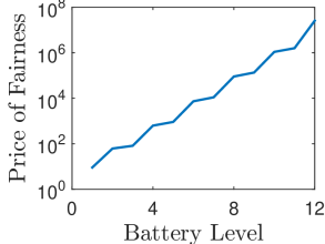
(a) $P_{1}=$ $\left[\begin{smallmatrix}0.95&0.05\\ 0.95&0.05\end{smallmatrix}\right]$,
$P_{2}=$$\left[\begin{smallmatrix}0.51&0.49\\ 0.51&0.49\end{smallmatrix}\right]$

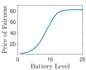
(b) $P_{1}=$  $\left[\begin{smallmatrix}0.9&0.1\\ 0.9&0.1\end{smallmatrix}\right]$,
     $P_{2}=$  $\left[\begin{smallmatrix}0.51&0.49\\ 0.51&0.49\end{smallmatrix}\right]$, $P_{3}=$ $\left[\begin{smallmatrix}0.55&0.45\\ 0.55&0.45\end{smallmatrix}\right]$

Figure 1: These figures show the change in price of fairness as battery size increases when the sources are independent. $S=\{-1,1\}^{n}$ and $P_{i}$ denotes the transition matrix of source $i$.

An example of the phenomenon of unbounded PoF when all sources are net generating is shown in Figure 1(a). Note that the above theorem does not show that the PoF for a given net generation profile grows to infinity as $b_{\max}\rightarrow\infty;$ see Figure 1(b), where PoF seems to saturate with increasing $b_{\max}.$

V Optimizing Fairness Subject to Efficiency

It is clear from Section IV that there exist cases, in which the Price of Fairness becomes unbounded as battery size increases. In this section, we formulate a problem in which we try to maximize fairness subject to efficiency, i.e., we pose being efficient as a hard constraint and ask how fair can we get?

We first define the objective which captures the fairness in the system. Our notion of fairness is to minimize the maximum over all users, the amount a user draws minus the amount it supplies to the battery. Recall the net contribution C${}_{i}=\lim_{T\rightarrow\infty}\frac{1}{T}\sum_{t=0}^{T}\mathbb{E}[A_{i}(t)]$ of user $i$ defined in Section III. Now, by work conservation we have under any policy, $\sum_{i\in[n]}{\rm C}_{i}=0$. The system is said to be completely fair when ${\rm C}_{i}=0\ \forall i\in[n]$. In general, this may not be the case. Hence to maximize fairness, we maximize the minimum of ${\rm C}_{i}$.

Here, by being efficient, we mean being in the space of policies which minimize the LLR without the hard fairness constraint. In general, the optimal value of an objective, in this case fairness, over an arbitrary set of policies is not easily computable. However, an observation we made in Section IV allows to formulate this as a tractable problem. Recall from Section IV that efficient policies are those that take actions in the space $A_{e}(x,b)$ when the state is $(x,b)\in{\bf S}.$ As a consequence, the space of efficient policies can be described by specifying only the space of allowable actions. This allows us to formulate this problem as a CMDP.

Thus, we define the problem of maximizing fairness subject to efficiency as follows

$$\max_{\phi\in\Phi_{e}}\min_{i\in[n]}\lim_{T\rightarrow\infty}\frac{1}{T}\sum_{t=0}^{T}\mathbb{E}[A_{i}(t)],$$ (8)

where the maximization is over all $\phi$ that are efficient, i.e., that are constrained to take actions in $A_{e}(x,b)$ in every state $(x,b).$ This problem can also be formulated as a CMDP as follows

(F) $$\mathop{\hbox{\rm maximize}}_{\phi,\theta}$$

subject to

V-A Reduction to a Linear Program

The optimization problem (F) above is extremely complex since the class of all history dependent policies is a highly unstructured space. This makes it extremely hard to derive a policy or a battery management algorithm. However, a remarkable simplification is possible, which allows for the computation of such policies in an efficient manner.

A Markov decision process is said to be unichain if, under any stationary deterministic policy, the corresponding Markov chain contains a single (aperiodic) ergodic class. This ensures the existence of a unique stationary distribution, independent of the initial distribution. Notice that under any policy $\phi\in\Phi_{e}$ the battery dynamics are identical and deterministic. Consequently, under any policy $\phi\in\Phi_{e}$, the Markov chain $(X(t),b(t))$ has a single ergodic class, making this CMDP unichain. A well-known fact about unichain CMDPs is that stationary randomized policies dominate (see, e.g., Theorem 4.1 of [9]); thanks to this, we can limit our search to stationary randomized policies. Moreover, the CMDP admits an elegant equivalent linear programming formulation (Theorem 4.3 of [9]), where the optimization is not over policies, but rather over occupation measures (or probability distributions) on the product of state and action spaces. We introduce this formulation below.

An occupation measure $\rho$ is a probability distribution on ${\bf S}\times{\bf A}_{e}$, where ${\bf A}_{e}=\bigcup_{(x,b)\in{\bf S}}A_{e}(x,b)$. In the LP formulation, the occupation measure is required to satisfy,

$$\sum_{(x,b)\in{\bf S}}\sum_{a\in A_{e}(x,b)}\rho(x,b,a)=1,\quad\rho(x^{\prime},b^{\prime},a^{\prime}) \geq 0,$$ (9)

$$\sum_{(x,b)\in{\bf S}}\sum_{a\in A_{e}(x,b)}\rho(x,b,a)(\delta_{(x^{\prime},b^{\prime})}(x,b)-P(x^{\prime},b^{\prime}|a,x,b)) =0$$ (10)

$\forall(x^{\prime},b^{\prime})\in{\bf S},a^{\prime}\in{\bf A}_{e}$, where,

$$\delta_{(u,v)}(u^{\prime},v^{\prime})=\begin{cases}1,&{\rm if}\ u=u^{\prime}\ {\rm and}\ v=v^{\prime},\\ 0,&{\rm otherwise,}\end{cases}$$

and $P(x^{\prime},b^{\prime}|a,x,b)$ is the probability of transition from state $(x,b)$ to state $(x^{\prime},b^{\prime})$ under action $a\in A_{e}(x^{\prime},b^{\prime})$. In our case, these dynamics are trivial:

$$P(x^{\prime},b^{\prime}|a,x,b)=P(x^{\prime}|x)\mathbb{I}\{b^{\prime}=b+\sum_{i\in[n]}a_{i}\},$$

and $P(x^{\prime}|x)$ is the probability that the background process $X(t)$ transitions from $x$ to $x^{\prime}$. (9) encodes that $\rho$ is a probability distribution on ${\bf S}\times{\bf A}_{e}.$ (10) imposes that $\rho$ is an invariant distribution for the controlled Markov chain.

The equivalent LP formulation of (F) is then given by [9]:

(LP) $$\mathop{\hbox{\rm maximize}}_{\rho,\theta}$$

subject to

Here, $\rho_{e}$ is the set of $\rho$ that satisfy (9)-(10), and with a slight abuse of notation, we define

$$\rho(a_{i}=u) =\underset{(x,b,a)\in{\bf S}\times{\bf A}_{e}:\ a_{i}=u}{\sum}\rho(x,b,a).$$

The first constraint in (LP) arises from the fairness definition, restated using occupation measures. This formulation allows for efficient computation of the optimal fairness. We next prove a result giving structural properties of efficient policies.

Proposition V.1

Under any efficient policy, the battery dynamics remain the same. Moreover, the underlying marginal distribution over states ($\rho(x,b)\ \forall x,b\in{\bf S}$) is the same across efficient policies.

Proof:

Using E1, E2 and E3, we note that irrespective of what actions we choose for each agent, the sum total of all actions in $A_{e}(x,b)$ is the same for each pair $(x,b)\in{\bf S}$. Since the battery dynamics are $b(t+1)=b(t)+\sum_{i}a_{i}(t)$, the battery dynamics stay the same across efficient policies.

Using the first claim, we can see that the transition matrix for $(x,b)$ is the same across all efficient policies. Thus, $\rho(x,b)$ is the same across all efficient policies.  

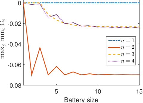
Figure 2: This figure shows how the maxmin fairness varies with increasing battery size. $S=\{-1,1\}^{n}$ and $P_{i}$ denotes the transition matrix of source $i$. We have the following sources and $n=k$ implies a system which has first $k$ of these sources.
$P_{1}=$ $\left[\begin{smallmatrix}0.5&0.5\\ 0.6&0.4\end{smallmatrix}\right]$ , $P_{2}=$ $\left[\begin{smallmatrix}0.5&0.5\\ 0.8&0.2\end{smallmatrix}\right]$ , $P_{3}=$ $\left[\begin{smallmatrix}0.7&0.3\\ 0.7&0.3\end{smallmatrix}\right]$ , $P_{4}=$ $\left[\begin{smallmatrix}0.8&0.2\\ 0.4&0.6\end{smallmatrix}\right]$.

We have computed the solution to (LP) and the plot of optimal fairness with increasing battery size for different user configurations is given in footnote 3. We have taken the background processes of the users to be independent for these evaluations. From this plot, we can observe that the fairness tends to saturate on increasing battery size, i.e. after a certain threshold, the fairness value approaches a negative constant (except for the case $n=1,$ where the efficient policy is also fair). This illustrates that increasing the battery size does not necessarily improve the fairness of efficient policies.

footnote 3 indicates that even a relaxation of the fairness constraint in (P) to C${}_{i}\geq-\delta$ for some $\delta>0$ is not guaranteed to result in an efficient battery operation, even as $b_{\max}\rightarrow\infty.$ To illustrate this explicitly, in Figure 3(a) and Figure 3(b), we plot the fairness efficiency frontier for 3 and 5 users, respectively. These plots show how close we get to efficient operation by relaxing the fairness constraint from C${}_{i}\geq 0$ to C${}_{i}\geq-\delta\ \forall i$. The shaded region shows all those points which are achievable and the frontier is the boundary for the achievable region. For the case when an efficient policy is fair, the frontier would coincide with the axes.

This reveals a fundamental conflict between efficiency and fairness: a small relaxation of the fairness constraint does not necessarily improve efficiency, and a small relaxation of the efficiency requirement does not necessarily imply fairness for all users (this follows from our previous observation of unbounded PoF).

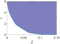
(a) $P_{1}=$ $\left[\begin{smallmatrix}0.6&0.4\\ 0.6&0.4\end{smallmatrix}\right]$, $P_{2}=\$ $\left[\begin{smallmatrix}0.9&0.1\\ 0.9&0.1\end{smallmatrix}\right]$, $P_{3}=$ $\left[\begin{smallmatrix}0.6&0.4\\ 0.5&0.5\end{smallmatrix}\right]$

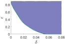
(b) $P_{1}=$ $\left[\begin{smallmatrix}0.7&0.3\\ 0.4&0.6\end{smallmatrix}\right]$, $P_{2}=$ $\left[\begin{smallmatrix}0.6&0.4\\ 0.9&0.1\end{smallmatrix}\right]$, $P_{3}=$ $\left[\begin{smallmatrix}0.6&0.4\\ 0.2&0.8\end{smallmatrix}\right]$, $P_{4}=$ $\left[\begin{smallmatrix}0.8&0.2\\ 0.8&0.2\end{smallmatrix}\right]$, $P_{5}=$ $\left[\begin{smallmatrix}0.51&0.49\\ 0.51&0.49\end{smallmatrix}\right]$.

Figure 3: These figures show the fairness efficiency frontier for 3 and 5 users respectively with $b_{\max}=12$, $S=\{-1,1\}^{n}$ and $P_{i}$ denotes the transition matrix of source $i$. This optimal loss of load is denoted by ${\rm LLR}_{\delta}$. The plot is of $\epsilon$ v/s $\delta$, where $\epsilon=\frac{{\rm LLR}_{\delta}}{{\rm LLR}_{e}}-1$. and the fairness constraints are $C_{i}\geq-\delta$.

To concretize our claim regarding the fundamental conflict between efficiency and fairness, we show in the following example that irrespective of the battery level, any efficient policy always has a non-zero maxmin fair value. We consider a setup of two users, wherein each user either generates unit power or demands unit power at each time instant. Let the transition probability matrix of user $i$ be given by

$$P_{i}=\left[\begin{matrix}p_{i}&1-p_{i}\\ 1-q_{i}&q_{i}\end{matrix}\right].$$ (11)

Then, we define the generation probability of user $i$ by $\alpha_{i}=\frac{1-q_{i}}{2-p_{i}-q_{i}}$. Using this setup, we give the following proposition, which gives a class of examples where the fairness remains bounded away from zero under efficient policies. We denote the maxmin fair value under efficient policies by F_e.

Proposition V.2

Consider two users with $S=\{-1,1\}^{2}$ and the transition probability matrix of user $i$ being $P_{i}$ (as in 11). If $\alpha_{1}>\alpha_{2}$, we have F${}_{e}=\alpha_{2}-\alpha_{1}$ for all even battery sizes.

Proof:

First, we note that $\rho(b=k)=0$ for $k$ odd. This is because, for even battery size, we know that in the long run the battery spends only finite amount of time in the odd battery levels and spends an infinite amount of time in the even battery levels. To see this, at each even battery level, we either accept two units of power, accept one unit and give one unit, or supply two units of power. Thus the battery level doesn’t change it’s parity unless it hits a boundary. If the battery level is initially odd, we know that it will hit either the upper boundary ($b_{\max}$) or the lower boundary $(0)$ in finite time, both of which are even. After this, the battery level stays even.

Let $\alpha_{i}$ denote the generation probability of user $i$ and let $\alpha_{i}^{\prime}=1-\alpha_{i}$. Let $\rho(\cdot,\cdot)$ denote the occupation measure of states of any efficient policy (Prop. V.1). We note that given that the policy is efficient, from E1,E2 and E3, the freedom in the action is only when the background state is $x=(-1,-1)$ and the battery level is $b=1$ and when the background state is $x=(1,1)$ and the battery level is $b=b_{\max}-1$. Let us assume that when the background state is $x=(-1,-1)$ and the battery level is $b=1$, we choose action $a=(-1,0)$ with probability $s$ and action $a=(0,-1)$ with probability $1-s$. Also, assume that when the background state is $x=(1,1)$ and the battery level is $b=b_{\max}-1$, we choose action $a=(1,0)$ with probability $t$ and action $a=(0,1)$ with probability $1-t$. Thus, we have,

$${\rm C}_{1}-{\rm C}_{2}= 2(\alpha_{1}-\alpha_{2})+(2t-1)\rho(x=(1,1),b=b_{\max}-1)$$

$$-(2s-1)\rho(x=(-1,-1),b=1).$$

Since $\rho(b=k)=0$ for $k$ odd, we have ${\rm C}_{1}-{\rm C}_{2}=2(\alpha_{1}-\alpha_{2}).$ Thus, we have C${}_{1}=\alpha_{1}-\alpha_{2}$ and C${}_{2}=\alpha_{2}-\alpha_{1}$. For $\alpha_{1}>\alpha_{2}$, C${}_{2}<$ C₁ and hence F${}_{e}=\alpha_{2}-\alpha_{1}$ for all even battery sizes.  

VI Concluding Remarks and Future Work

We studied the problem of scheduling of a shared energy storage among multiple users by concentrating on the tradeoff between fairness of use across users and the efficiency of use of the battery. Our results show that there are hard fundamental limits to fairness under efficiency constraints and to efficiency under fairness constraints. In particular, a larger battery size does not help in achieving both fairness and efficiency simultaneously. Our effort at characterizing these tradeoffs was via optimization of efficiency subject to fairness (and vice-versa). We have also simulated the fairness-efficiency frontier of levels of efficiency and fairness that cannot be jointly improved upon under any policy or battery size. Our results also indicate that sharing contracts and costing of batteries should be done with care since fair operations imply suboptimal battery utilization. Devising an equitable sharing of costs and a market for transacting excess energy are fascinating directions of future research.

Appendix A Large battery asymptotics for a single user

In this section, we consider the problem of minimizing the LLR associated with a single user $i$ operating a battery of size $b_{\max}$ alone. We make the following remarks:

1. The net generation process $X_{i}(\cdot)$ corresponding to user $i$ is a functional of the DTMC $X(\cdot).$

2. An elementary energy conservation argument shows that any policy of battery operation for user $i$ is fair with respect to the fairness notion (5).

3. The LLR of user $i$ is minimized by a simple greedy policy: Suppose that the net generation is $x_{i}$ and the battery occupancy equals $b.$ If $0\leq b+x\leq b_{\max}$, set action $a=x.$ If $b+x<0$, set $a=-b,$ and if $b+x>b_{\max}$, set $a=b_{\max}-b$. Under this policy, the battery evolution is given by

   $$B(t+1)=[B(t)+X_{i}(t)]_{[0,b_{\max}]},$$ (12)

   where $[z]_{[0,b_{\max}]}=\min(\max(z,0),b_{\max}).$

The main result of this section is that if $\Delta_{i}>0,$ then ${\rm LLR}_{o,i},$ the optimal LLR for user $i,$ decays exponentially with the battery size $b_{\max}.$

Theorem A.1

For user $i$ operating a battery of size $b_{\max}$ in a standalone fashion, if $\Delta_{i}>0,$ then

$$\lim_{b_{\max}\rightarrow\infty}\frac{\log({\rm LLR}_{o,i})}{b_{\max}}=-\lambda_{i},$$

where $\lambda_{i}\in(0,\infty).$

Theorem A.1 is a consequence of the following lemmas.

Lemma A.1

Let the setting of Theorem A.1 hold. Under the battery evolution given by (12),

$$\lim_{b_{\max}\rightarrow\infty}\frac{\log({\rm LLR}_{o,i})}{b_{\max}}=\lim_{b_{\max}\rightarrow\infty}\frac{\log\mathbb{P}\left[B=0\right]}{b_{\max}}.$$

where $B$ is distributed according to the steady state distribution of $B(\cdot)$

Proof:

It is easy to see that ${\rm LLR}_{o,i}\leq\mathbb{P}\left[B=0\right].$ It therefore suffices to show that ${\rm LLR}_{o,i}\geq c\mathbb{P}\left[B=0\right]$ for some $c\in(0,1).$ This is a direct consequence of our assumption that $\mathbb{P}\left[X(t+1)=s\ |\ X(t)=s\right]>0$ for all $s\in S,$ which ensures that each time the battery drains to zero, there is positive probability of a loss of load. This argument can be easily formalized using the renewal reward theorem.  

Lemma A.2

Let the setting of Theorem A.1 hold. Under the battery evolution given by (12),

$$\lim_{b_{\max}\rightarrow\infty}\frac{\log\mathbb{P}\left[B=0\right]}{b_{\max}}=-\lambda_{i},$$

where $\lambda_{i}\in(0,\infty).$

Proof:

We analyse the asymptotics of $\mathbb{P}\left[b=0\right]$ using the reversed system [11], which is obtained by interchanging the role of generation and demand. In other words, $X_{i}^{r}(t)=-X_{i}(t)$ (we use the superscript $r$ to represent quantities in the reversed system). Thus, $\Delta_{i}^{r}=-\Delta_{i}<0.$ It is not hard to see that

$$\mathbb{P}\left[B=0\right]=\mathbb{P}\left[B^{r}=b_{\max}\right].$$

The battery evolution in the reversed system is equivalent to the buffer evolution in a finite buffer Markov modulated queue with negative drift, for which logarithmic asymptotics of the form

$$\lim_{b_{\max}\rightarrow\infty}\frac{\log\mathbb{P}\left[B^{r}=b_{\max}\right]}{b_{\max}}=-\lambda$$

are known; see [12, Section 6.5] and [13].  

Karan N. Chadha Karan is a dual degree student of Electrical Engineering at Indian Institute of Technology Bombay (IITB). His research interests include applied probabilty, game theory, optimization and learning theory.

Ankur A. Kulkarni Ankur is an Associate Professor with the Systems and Control Engineering group at Indian Institute of Technology Bombay (IITB). He received his B.Tech. from IITB in 2006, M.S. in 2008 and Ph.D. in 2010, both from the University of Illinois at Urbana-Champaign (UIUC). From 2010-2012 he was a post-doctoral researcher at the Coordinated Science Laboratory at UIUC. His research interests include information theory, stochastic control, game theory, combinatorial coding theory problems, optimization and variational inequalities, and operations research. He was an Associate (from 2015–2018) of the Indian Academy of Sciences, Bangalore, a recipient of the INSPIRE Faculty Award of the Department of Science and Technology, Government of India, 2013, Best paper awards at the National Conference on Communications, 2017, Indian Control Conference, 2018 and International Conference on Signal Processing and Communications (SPCOM) 2018, Excellence in Teaching Award 2018 at IITB and the William A. Chittenden Award, 2008 at UIUC. He is a consultant to the Securities and Exchange Board of India on regulation of high frequency trading.

Jayakrishnan Nair Jayakrishnan received his BTech and MTech in Electrical Engg. (EE) from IIT Bombay (2007) and Ph.D. in EE from California Inst. of Tech. (2012). He has held post-doctoral positions at California Inst. of Tech. and Centrum Wiskunde & Informatica. He is currently an Assistant Professor in EE at IIT Bombay. His research focuses on modeling, performance evaluation, and design issues in queueing systems and communication networks.

References

- [1] K. N. Chadha, A. A. Kulkarni, and J. Nair, “Efficiency fairness tradeoff in battery sharing,” in Decision and Control (CDC), 2019 IEEE 58nd Annual Conference on. IEEE, 2019, p. pages.
- [2] D. Kalathil, C. Wu, K. Poolla, and P. Varaiya, “The sharing economy for the electricity storage,” IEEE Transactions on Smart Grid, vol. 10, no. 1, pp. 556–567, jan 2019. [Online]. Available: https://doi.org/10.1109/tsg.2017.2748519
- [3] P. Chakraborty, E. Baeyens, K. Poolla, P. P. Khargonekar, and P. Varaiya, “Sharing storage in a smart grid: A coalitional game approach,” IEEE Transactions on Smart Grid, pp. 1–1, 2018. [Online]. Available: https://doi.org/10.1109/tsg.2018.2858206
- [4] C. Wu, J. Porter, and K. Poolla, “Community storage for firming,” in 2016 IEEE International Conference on Smart Grid Communications (SmartGridComm). IEEE, nov 2016. [Online]. Available: https://doi.org/10.1109/smartgridcomm.2016.7778822
- [5] Y. H. Zhou, A. Scheller-Wolf, N. Secomandi, and S. Smith, “Managing wind-based electricity generation in the presence of storage and transmission capacity,” Production and Operations Management, nov 2018. [Online]. Available: https://doi.org/10.1111/poms.12946
- [6] J. H. Kim and W. B. Powell, “Optimal energy commitments with storage and intermittent supply,” Operations Research, vol. 59, no. 6, pp. 1347–1360, dec 2011. [Online]. Available: https://doi.org/10.1287/opre.1110.0971
- [7] M. Korpaas, A. T. Holen, and R. Hildrum, “Operation and sizing of energy storage for wind power plants in a market system,” International Journal of Electrical Power & Energy Systems, vol. 25, no. 8, pp. 599–606, oct 2003. [Online]. Available: https://doi.org/10.1016/s0142-0615(03)00016-4
- [8] P. M. van de Ven, N. Hegde, L. Massoulié, and T. Salonidis, “Optimal control of end-user energy storage,” IEEE Transactions on Smart Grid, vol. 4, 03 2012.
- [9] E. Altman, Constrained Markov Decision Processes, 1999.
- [10] M. L. Puterman, Markov decision processes: discrete stochastic dynamic programming. John Wiley & Sons, 2014.
- [11] D. Mitra, “Stochastic theory of a fluid model of producers and consumers coupled by a buffer,” Advances in Applied Probability, vol. 20, no. 3, pp. 646–676, 1988.
- [12] A. J. Ganesh, N. O’Connell, and D. J. Wischik, Big queues. Springer, 2004.
- [13] F. Toomey, “Bursty traffic and finite capacity queues,” Annals of Operations Research, vol. 79, pp. 45–62, 1998.