Model-Free Stochastic Reachability Using Kernel Distribution Embeddings

Abstract

We present a data-driven solution to the terminal-hitting stochastic reachability problem for a Markov control process. We employ a nonparametric representation of the stochastic kernel as a conditional distribution embedding within a reproducing kernel Hilbert space (RKHS). This representation avoids intractable integrals in the dynamic recursion of the stochastic reachability problem since the expectations can be calculated as an inner product within the RKHS. We demonstrate this approach on a high-dimensional chain of integrators and on Clohessy-Wiltshire-Hill dynamics.

I Introduction

Stochastic reachability is an established verification tool to assure that a system will reach a desired state without violating predefined safety constraints with at least a desired likelihood. The solution to the stochastic reachability problem is based on dynamic programming [1, 2], which poses significant computational challenges. Optimization-based solutions have garnered modest computational tractability via chance constraints [3, 4], sampling methods [5, 6, 7], and convex optimization with Fourier transforms [8, 9], but are limited to linear dynamical systems with Gaussian or log-concave disturbances. Methods using approximate dynamic programming [10] and particle filtering [11, 3], are applicable to classes of nonlinear systems, but have only been demonstrated on systems with moderate dimensionality.

Further, for many dynamical systems, presumption of accurate knowledge of dynamics and uncertainty is unrealistic. Historically, such uncertainty is handled through approximations and introduction of error terms that bound unknown elements [12, 13]. With the rapid increase in the use of learning elements that are resistant to traditional models for control and formal methods, as well as the involvement of humans, such approaches may either be overly conservative or even simply inaccurate. For example, human inputs may be highly heterogeneous, may not follow a known distribution, and are often data-driven processes that may be biased when analyzed through sampling methods.

We propose to use conditional distribution embeddings within a reproducing kernel Hilbert space (RKHS) to solve the stochastic reachability problem. As a tool for stochastic reachability, kernel methods offer significant advantages over state-of-the-art: 1) they are model-free, so can accommodate data-driven stochastic processes and nonlinear dynamics, 2) they are convergent in probability, and 3) they do not suffer from the curse of dimensionality [14] or from issues of numerical quadrature that plague optimization based approaches. The primary computational challenge arises in the inversion of a matrix that scales with the number of data points, leading to computational complexity that is exponential in the size of the data.

Kernel methods are an established learning technique [15, 16, 17], and have recently been applied to dynamic programming problems with additive cost function and infinite time horizon [18]. Kernel methods broadly enable nonparametric inference using kernel embeddings of distributions. They can capture the features of arbitrary statistical distributions in a data-driven fashion [19, 20]. Kernel methods do not suffer from biases or prior assumptions on the system model, and are computationally efficient because they are convergent and non-iterative [15]. These techniques have also been applied to several problems in dynamical systems, including controller synthesis [21], partially-observable systems [22], and estimation of graphical models [23].

The main contribution of this paper is the application of conditional distribution embedding to compute the stochastic reachability probability measure, to enable model-free verification without invoking a statistical approach. This is particularly relevant for systems with black-box elements, such as autonomous or human-in-the-loop systems, which have traditionally been resistant to formal verification techniques. We tailor the approach in [18] to accommodate the multiplicative cost and finite horizon associated with the stochastic reachability dynamic program. We apply kernel methods to compute the stochastic reachability probability measure by representing the stochastic kernel as a conditional distribution embedding within an RKHS.

The paper organization is as follows. Section II formulates the problem. Section III applies conditional distribution embeddings to compute the stochastic reachability probability measure. Section IV demonstrates our approach on three examples: a double integrator to enable validation with a “truth” model via dynamic programming, a 10,000-dimensional integrator to demonstrate scalability, and spacecraft rendezvous and docking.

II Problem Formulation

For sets $\mathcal{A}$ and $\mathcal{B}$, the set of all elements of $\mathcal{A}$ which are not in $\mathcal{B}$ is denoted as $\mathcal{A}\backslash\mathcal{B}$. We denote the indicator function as $\boldsymbol{1}_{\mathcal{A}}(x)=1$ if $x\in\mathcal{A}$ and $\boldsymbol{1}_{\mathcal{A}}(x)=0$ if $x\notin\mathcal{A}$.

Let $\Omega$ denote a sample space and $\mathcal{F}(\Omega)$ denote the $\sigma$-algebra relative to $\Omega$. A probability measure $\mathop{\rm Pr}\nolimits$ assigned to the measurable space $(\Omega,\mathcal{F}(\Omega))$ is defined as the probability space $(\Omega,\mathcal{F}(\Omega),\mathop{\rm Pr}\nolimits)$. When $\Omega\equiv\Re$, the $\sigma$-algebra of $\Omega$ is denoted as $\mathscr{B}(\Omega)$, and is the Borel $\sigma$-algebra associated with $\Omega$. A random variable $\boldsymbol{x}$ is a measurable function on the probability space $(\Omega,\mathcal{F}(\Omega),\mathop{\rm Pr}\nolimits)$. A random vector $\boldsymbol{x}=[\boldsymbol{x}_{1},\ldots,\boldsymbol{x}_{n}]^{\top}$ of $n$ random variables $\{\boldsymbol{x}_{i}\}_{i=1}^{n}$, each measurable functions on the probability space $(\Omega,\mathcal{F}(\Omega),\mathop{\rm Pr}\nolimits)$, is defined on the induced probability space $(\Omega^{n},\mathcal{F}(\Omega^{n}),\mathop{\rm Pr}\nolimits_{\boldsymbol{x}})$, where $\mathop{\rm Pr}\nolimits_{\boldsymbol{x}}$ is the induced probability measure. A stochastic process is defined as a sequence of random vectors $\{\boldsymbol{x}_{k}:k\in[0,N]\}$, $N\in\mathbb{N}$, where $\boldsymbol{x}_{k}$ are defined on the probability space $(\Omega^{n},\mathcal{F}(\Omega^{n}),\mathop{\rm Pr}\nolimits_{\boldsymbol{x}})$. See [24, 25] for more details.

The expectation operator is denoted as $\mathbb{E}[\,\cdot\,]$, where for some function $f$, $\mathbb{E}_{\boldsymbol{x}\sim\mathop{\rm Pr}\nolimits_{\boldsymbol{x}}\{\,\cdot\,\}}[f(\boldsymbol{x})]$ denotes the expectation operator with respect to the probability measure $\mathop{\rm Pr}\nolimits_{\boldsymbol{x}}$.

II-A Terminal-Hitting Time Problem

Consider a Markov control process $\mathcal{H}$, which is defined in [1] as a 3-tuple,

$$\mathcal{H}=(\mathcal{X},\mathcal{U},Q)$$ (1)

where $\mathcal{X}\subseteq\Re^{n}$ is the state space, $\mathcal{U}\subseteq\Re^{m}$ is the control space, and $Q:\mathscr{B}(\mathcal{X})\times{}\mathcal{X}\times{}\mathcal{U}\rightarrow[0,1]$ is a stochastic kernel, which is a Borel-measurable function that maps a probability measure $Q(\,\cdot\,|\,x,u)$ to each $x\in\mathcal{X}$ and $u\in\mathcal{U}$ on the Borel space $(\mathcal{X},\mathscr{B}(\mathcal{X}))$. Further, let $\mathcal{X}$ and $\mathcal{U}$ be compact Borel spaces. The system evolves over a finite horizon $k\in[0,N]$ with inputs chosen according to a Markov policy [26, 27], a sequence $\pi=\{\pi_{0},\pi_{1},\ldots,\pi_{N-1}\}$ of universally-measurable maps $\pi_{k}:\mathcal{X}\rightarrow\mathcal{U}$. The set of all Markov control policies $\pi$ is denoted as $\mathcal{M}$.

We define $\mathcal{K},\mathcal{T}\in\mathscr{B}(\mathcal{X})$ as the safe set and target set, respectively. We define the terminal-hitting time safety probability $r_{x_{0}}^{\pi}(\mathcal{K},\mathcal{T})$ [1] as the probability that a system $\mathcal{H}$ controlled by a policy $\pi\in\mathcal{M}$ will reach $\mathcal{T}$ at $k=N$ while avoiding $\mathcal{X}\backslash\mathcal{K}$ for all $k\in[0,N-1]$, given an initial condition $x_{0}\in\mathcal{X}$.

$$r_{x_{0}}^{\pi}(\mathcal{K},\mathcal{T})\triangleq\mathop{\rm Pr}\nolimits_{x_{0}}^{\pi}\{\boldsymbol{x}_{N}\in\mathcal{T}\wedge{}\boldsymbol{x}_{i}\in\mathcal{K},\forall i\in[0,N-1]\}$$ (2)

Let $V{}_{k}^{\pi}:\mathcal{X}\rightarrow[0,1]$ be defined via backward recursion as

$$V{}_{N}^{\pi}(x) =\boldsymbol{1}_{\mathcal{T}}(x)$$ (3)

$$V{}_{k}^{\pi}(x) =\boldsymbol{1}_{\mathcal{K}}(x)\mathbb{E}_{\boldsymbol{y}\sim Q(\,\cdot\,|\,x,\pi_{k}(x))}\left[V{}_{k+1}^{\pi}(\boldsymbol{y})\right]$$ (4)

then $V{}_{0}^{\pi}(x)=r_{x_{0}}^{\pi}(\mathcal{K},\mathcal{T})$ for every $x_{0}\in\mathcal{X}$.

From [1, Definition 10], a policy $\pi^{*}\in\mathcal{M}$ is the maximal reach-avoid policy in the terminal sense if and only if

$$r_{x_{0}}^{\pi^{*}}(\mathcal{K},\mathcal{T})=\sup_{\pi\in\mathcal{M}}\{r_{x_{0}}^{\pi}(\mathcal{K},\mathcal{T})\}$$ (5)

Let $V{}_{k}^{*}:\mathcal{X}\rightarrow[0,1]$, $k\in[0,N-1]$ be defined via backward recursion, initialized with $V{}_{N}^{*}(x)=\boldsymbol{1}_{\mathcal{T}}(x)$, as

$$V{}_{k}^{*}(x)=\sup_{u\in\mathcal{U}}\left\{\boldsymbol{1}_{\mathcal{K}}(x)\mathbb{E}_{\boldsymbol{y}\sim Q(\,\cdot\,|\,x,u)}\left[V{}_{k+1}^{*}(\boldsymbol{y})\right]\right\}$$ (6)

Then, $V{}_{0}^{*}(x)=r_{x_{0}}^{\pi^{*}}(\mathcal{K},\mathcal{T})$. If $\pi^{*}$ is such that

$$\pi_{k}^{*}(x)=\mathrm{arg}\sup_{u\in\mathcal{U}}\left\{\boldsymbol{1}_{\mathcal{K}}(x)\mathbb{E}_{\boldsymbol{y}\sim Q(\,\cdot\,|\,x,u)}\left[V{}_{k+1}^{*}(\boldsymbol{y})\right]\right\}$$ (7)

then $\pi^{*}$ is maximal in the terminal sense [1, Theorem 11].

II-B Problem Statement

Consider a set $\mathcal{S}$ of $M$ samples of the form $\mathcal{S}=\{(\bar{y}_{i},\bar{x}_{i},\bar{u}_{i})\}_{i=1}^{M}$ such that $y_{i}$ is drawn i.i.d. from $Q$ according to $\bar{y}_{i}\sim Q(\,\cdot\,|\,\bar{x}_{i},\bar{u}_{i})$, and $\bar{u}_{i}=\pi(\bar{x}_{i})$. We denote sample vectors with a bar to differentiate them from time-indexed vectors.

Problem 1.

Without direct knowledge of $Q$, use samples $\mathcal{S}$ to construct a kernel-based approximation of (4) that converges in probability.

Problem 2.

Without direct knowledge of $Q$, use samples $\mathcal{S}$ to construct a kernel-based approximation of (6) that converges in probability, in order to compute an approximation of the optimal policy $\pi^{*}$.

Using samples $\mathcal{S}$, we employ an approach similar to that in [18], but that is specific to the dynamic program associated with the stochastic reachability problem for high-dimensional, non-Gaussian systems. The unique computational efficiencies afforded by reproducing kernel Hilbert spaces transforms computation of (4) and (6) into simple matrix operations and inner products.

III Kernel Distribution Embeddings for Stochastic Reachabilty

For some set $\mathcal{X}$, let $\mathscr{H}_{\mathcal{X}}$ denote the unique reproducing kernel Hilbert space [15] with the positive definite [28, Definition 4.15] kernel $K_{\mathcal{X}}:\mathcal{X}\times{}\mathcal{X}\rightarrow\Re$, which is a Hilbert space of real-valued functions on $\mathcal{X}$ with inner product $\langle\,\cdot,\cdot\,\rangle_{\mathscr{H}_{\mathcal{X}}}$ and the induced norm $\lVert x\rVert_{\mathscr{H}_{\mathcal{X}}}=\left(\langle x,x\rangle_{\mathscr{H}_{\mathcal{X}}}\right)^{1/2}$. A reproducing kernel Hilbert space has two important properties [17]:

1. For any $x,x^{\prime}\in\mathcal{X}$, $K_{\mathcal{X}}(x,\cdot\,):x^{\prime}\rightarrow K_{\mathcal{X}}(x,x^{\prime})$ is an element of $\mathscr{H}_{\mathcal{X}}$.

2. An element $K_{\mathcal{X}}(x,x^{\prime})$ of $\mathscr{H}_{\mathcal{X}}$ satisfies the reproducing property such that $\forall f\in\mathscr{H}_{\mathcal{X}}$ and $x\in\mathcal{X}$,

   $$f(x) =\langle K_{\mathcal{X}}(x,\cdot),f(\cdot)\rangle_{\mathscr{H}_{\mathcal{X}}}$$ (8)

   $$K_{\mathcal{X}}(x,x^{\prime}) =\langle K_{\mathcal{X}}(x,\cdot),K_{\mathcal{X}}(x^{\prime},\cdot)\rangle_{\mathscr{H}_{\mathcal{X}}}$$ (9)

This means that the evaluation of a function $f\in\mathscr{H}_{\mathcal{X}}$ can be viewed as an inner product in $\mathscr{H}_{\mathcal{X}}$. Alternatively, an element $K_{\mathcal{X}}(x,\cdot)$ can be viewed as a nonlinear feature map $\phi:\mathcal{X}\rightarrow\mathscr{H}_{\mathcal{X}}$, such that

$$K_{\mathcal{X}}(x,x^{\prime})=\langle\phi(x),\phi(x^{\prime})\rangle_{\mathscr{H}_{\mathcal{X}}}$$ (10)

Because constructing the feature map $\phi(\,\cdot\,)$ and computing $\langle\phi(x),\phi(x^{\prime})\rangle_{\mathscr{H}_{\mathcal{X}}}$ explicitly can be computationally expensive, the inner product can be computed using $K_{\mathcal{X}}(x,x^{\prime})$ directly for a $K_{\mathcal{X}}$ that is positive definite. This is known as the kernel trick [16].

By choosing $K_{\mathcal{X}}$, we effectively choose a basis to represent the functions in $\mathscr{H}_{\mathcal{X}}$. With the reproducing property, we can then write the function $f$ as $f(x)=w^{\top}\phi(x)$, a weighted sum of basis functions for some possibly infinite-dimensional weight vector $w$. We wish to solve for the particular $w$ which, based on the samples $\mathcal{S}$, minimizes the difference between the observations and the kernel-based estimate.

Let $\mathscr{P}$ denote the set of all probability measures on $\mathcal{X}$. The kernel distribution embedding [29, 20] of a probability measure $\mathop{\rm Pr}\nolimits_{\boldsymbol{y}\,|\,x,u}\in\mathscr{P}$, given by $\mu_{(x,u)}:\mathscr{P}\rightarrow\mathscr{H}_{\mathcal{X}}$, is defined as

$$\mu_{(x,u)}\triangleq\int_{\mathcal{X}}K_{\mathcal{X}}(y,\cdot)\mathop{\rm Pr}\nolimits_{\boldsymbol{y}\,|\,x,u}\{\mathrm{d}y\,|\,x,u\}$$ (11)

Let $\mathscr{H}_{\mathcal{X}}$ denote the unique RKHS for the state space $\mathcal{X}$ with the positive definite kernel $K_{\mathcal{X}}:\mathcal{X}\times{}\mathcal{X}\rightarrow\Re$. Similarly, let $\mathscr{H}_{\mathcal{X}\times\mathcal{U}}$ denote the RKHS for $\mathcal{X}\times\mathcal{U}$ with the positive definite kernel $K_{\mathcal{X}\times\mathcal{U}}:(\mathcal{X},\mathcal{U})\times{}(\mathcal{X},\mathcal{U})\rightarrow\Re$. We define the conditional distribution embedding of the stochastic kernel $Q\in\mathscr{P}$ as $\mu_{(x,u)}$. Then, the expectation of $f$ with respect to the probability measure $Q$ is given by

$$\langle\mu_{(x,u)},f\rangle_{\mathscr{H}_{\mathcal{X}}}=\mathbb{E}_{\boldsymbol{y}\sim Q(\,\cdot\,|\,x,u)}[f(\boldsymbol{y})]$$ (12)

This means we can evaluate the expectation of a function with respect to $Q$ as an inner product in $\mathscr{H}_{\mathcal{X}}$.

We can construct an estimate $\bar{\mu}_{(x,u)}$ of $\mu_{(x,u)}$ [20] from samples $\mathcal{S}$ to approximate (12),

$$\langle\bar{\mu}_{(x,u)},f\rangle_{\mathscr{H}_{\mathcal{X}}}\approx\mathbb{E}_{\boldsymbol{y}\sim Q(\,\cdot\,|\,x,u)}\left[f(\boldsymbol{y})\right]$$ (13)

According to the Riesz representation theorem [30], the element $\bar{\mu}_{(x,u)}$ can be viewed as the solution to a regularized least-squares problem that minimizes the error of the expectation operator over the samples [30, 31],

$$\min_{\bar{\mu}}\left\{\frac{1}{M}\sum_{i=1}^{M}\lVert K_{\mathcal{X}}(\bar{y}_{i},\cdot)-\bar{\mu}_{(\bar{x}_{i},\bar{u}_{i})}\rVert_{\mathscr{H}_{\mathcal{X}}}^{2}+\lambda\lVert\bar{\mu}\rVert_{\mathscr{H}_{\Upsilon}}^{2}\right\}$$ (14)

where $\mathscr{H}_{\Upsilon}$ is a vector-valued RKHS [30]. The solution is unique and has the form

$$\bar{\mu}_{(x,u)}=\eta\Phi^{\top}(G+\lambda MI)^{-1}\Psi K_{\mathcal{X}\times\mathcal{U}}((x,u),\cdot)$$ (15)

where $\lambda$ is a regularization parameter to avoid overfitting, $\eta$ is a normalizing constant, and $\Phi$, $\Psi$, and $G$ are defined as

$$\Phi =[K_{\mathcal{X}}(\bar{y}_{1},\cdot),\ldots,K_{\mathcal{X}}(\bar{y}_{M},\cdot)]^{\top}$$ (16)

$$\Psi =[K_{\mathcal{X}\times\mathcal{U}}((\bar{x}_{1},\bar{u}_{1}),\cdot),\ldots,K_{\mathcal{X}\times\mathcal{U}}((\bar{x}_{M},\bar{u}_{M}),\cdot)]^{\top}$$ (17)

$$G =\Psi\Psi^{\top}$$ (18)

By the reproducing property of $K_{\mathcal{X}}$ in $\mathscr{H}_{\mathcal{X}}$, $\forall f\in\mathscr{H}_{\mathcal{X}}$, we can rewrite (13) as

$$\langle\bar{\mu}_{(x,u)},f\rangle_{\mathscr{H}_{\mathcal{X}}} =\boldsymbol{f}^{\top}\beta(x,u)$$ (19)

where $\boldsymbol{f}=[f(\bar{y}_{1}),\ldots,f(\bar{y}_{M})]^{\top}$, and $\beta(x,u)\in\Re^{M}$ is a vector of coefficients,

$$\beta(x,u) =\eta(G+\lambda MI)^{-1}\Psi K_{\mathcal{X}\times\mathcal{U}}((x,u),\cdot)$$ (20)

This means an approximation of the value function expectation $\mathbb{E}_{\boldsymbol{y}\sim Q(\,\cdot\,|\,x,\pi_{k}(x))}\left[V{}_{k+1}^{\pi}(\boldsymbol{y})\right]$ in (4) can be evaluated as a linear operation in $\mathscr{H}_{\mathcal{X}}$.

III-A Terminal-Hitting Time Problem

With the conditional distribution embedding $\mu_{(x,u)}$, the value functions in (4) can be written as

$$V{}_{k}^{\pi}(x)=\boldsymbol{1}_{\mathcal{K}}(x)\langle\mu_{(x,\pi_{k}(x))},V{}_{k+1}^{\pi}\rangle_{\mathscr{H}_{\mathcal{X}}}$$ (21)

With the estimate $\bar{\mu}_{(x,u)}$ (15), we define the approximate value functions $\mkern 1.5mu\overline{\mkern-1.5muV\mkern-1.5mu}\mkern 1.5mu_{k}^{\pi}:\mathcal{X}\rightarrow[0,1]$, $k\in[0,N-1]$, as

$$\mkern 1.5mu\overline{\mkern-1.5muV\mkern-1.5mu}\mkern 1.5mu_{k}^{\pi}(x)=\boldsymbol{1}_{\mathcal{K}}(x)\langle\bar{\mu}_{(x,\pi_{k}(x))},V{}_{k+1}^{\pi}\rangle_{\mathscr{H}_{\mathcal{X}}}$$ (22)

such that $\mkern 1.5mu\overline{\mkern-1.5muV\mkern-1.5mu}\mkern 1.5mu_{k}^{\pi}(x)\approx V{}_{k}^{\pi}(x)$. Thus, an approximation for the reach-avoid probability $r_{x_{0}}^{\pi}(\mathcal{K},\mathcal{T})$ can be computed via the backward recursion described in Algorithm 1, such that

$$\mkern 1.5mu\overline{\mkern-1.5muV\mkern-1.5mu}\mkern 1.5mu_{0}^{\pi}(x)\approx r_{x_{0}}^{\pi}(\mathcal{K},\mathcal{T})$$ (23)

Algorithm 1 Value Function Estimate

Input: samples $\mathcal{S}$ drawn i.i.d. from $Q$, policy $\pi$, horizon $N$
Output: value function estimate $\mkern 1.5mu\overline{\mkern-1.5muV\mkern-1.5mu}\mkern 1.5mu_{0}^{\pi}(x)$

1:Compute $\Phi$ and $\Psi$ using $\mathcal{S}$ from (16) and (17)

2:$G\leftarrow\Psi\Psi^{\top}$

3:Initialize $\mkern 1.5mu\overline{\mkern-1.5muV\mkern-1.5mu}\mkern 1.5mu_{N}^{\pi}(x)\leftarrow\boldsymbol{1}_{\mathcal{T}}(x)$

4:for $k\leftarrow N-1$ to $0$ do

5:     Compute $\beta(x,\pi_{k}(x))$ from (20)

6:     $\mathcal{Y}\leftarrow[\mkern 1.5mu\overline{\mkern-1.5muV\mkern-1.5mu}\mkern 1.5mu_{k+1}^{\pi}(\bar{y}_{1}),\ldots,\mkern 1.5mu\overline{\mkern-1.5muV\mkern-1.5mu}\mkern 1.5mu_{k+1}^{\pi}(\bar{y}_{M})]^{\top}$

7:     $\mkern 1.5mu\overline{\mkern-1.5muV\mkern-1.5mu}\mkern 1.5mu_{k}^{\pi}(x)\leftarrow\boldsymbol{1}_{\mathcal{K}}(x)\mathcal{Y}^{\top}\beta(x,\pi_{k}(x))$

8:end for

9:Return $\mkern 1.5mu\overline{\mkern-1.5muV\mkern-1.5mu}\mkern 1.5mu_{0}^{\pi}(x)\approx r_{x_{0}}^{\pi}(\mathcal{K},\mathcal{T})$

We now seek to characterize the quality of the approximation and the conditions for its convergence. As in [32, 33, 34], we define a pseudometric that characterizes the accuracy of the estimate $\bar{\mu}_{(x,u)}$.

Definition 1 (Distance Pseudometric).

The distance pseudometric in $\mathscr{H}_{\mathcal{X}}$ between the conditional distribution embedding $\mu_{(x,u)}\in\mathscr{H}_{\mathcal{X}}$ and the estimate $\bar{\mu}_{(x,u)}\in\mathscr{H}_{\mathcal{X}}$ is defined as $\lVert\mu_{(x,u)}-\bar{\mu}_{(x,u)}\rVert_{\mathscr{H}_{\mathcal{X}}}$.

It is shown in [35] that if $K_{\mathcal{X}}$ is a characteristic, bounded kernel, then $\lVert\mu_{(x,u)}-\bar{\mu}_{(x,u)}\rVert_{\mathscr{H}_{\mathcal{X}}}=0$ if and only if $\mu_{(x,u)}=\bar{\mu}_{(x,u)}$. A kernel is characteristic if the kernel embedding is injective, meaning the embeddings for any two different conditional distributions are represented by different elements within the RKHS. Thus, as $\lVert\mu_{(x,u)}-\bar{\mu}_{(x,u)}\rVert_{\mathscr{H}_{\mathcal{X}}}$ converges [18, 20], the estimate converges in probability to the conditional distribution embedding within $\mathscr{H}_{\mathcal{X}}$.

Lemma 1.

[18, Lemma 2.2] For any $\varepsilon>0$, if the regularization parameter $\lambda$ in (14) is chosen such that $\lambda\rightarrow 0$ and $\lambda^{3}M\rightarrow\infty$, and if $\mathcal{X}$ is bounded and $K_{\mathcal{X}}$ is strictly positive definite, then

$$\mathop{\rm Pr}\nolimits_{\mathcal{S}\sim Q}\left\{\sup_{(x,u)\in\mathcal{X}\times\mathcal{U}}\lVert\mu_{(x,u)}-\bar{\mu}_{(x,u)}\rVert_{\mathscr{H}_{\mathcal{X}}}>\varepsilon\right\}\rightarrow 0$$ (24)

Proposition 2 (Value Function Convergence).

For any $\varepsilon>0$, if the regularization prameter $\lambda$ in (14) is chosen such that $\lambda\rightarrow 0$ and $\lambda^{3}M\rightarrow\infty$, and if $\mathcal{X}$ is bounded and $K_{\mathcal{X}}$ is strictly positive definite, $|V{}_{k}^{\pi}(x)-\mkern 1.5mu\overline{\mkern-1.5muV\mkern-1.5mu}\mkern 1.5mu_{k}^{\pi}(x)|$ converges in probability.

Proof.

By subtracting (22) from (21), and using the parallelogram law, we define the absolute value function error $\mathcal{E}_{k}(x)$ at time $k$,

$$\mathcal{E}_{k}(x) \triangleq|V{}_{k}^{\pi}(x)-\mkern 1.5mu\overline{\mkern-1.5muV\mkern-1.5mu}\mkern 1.5mu_{k}^{\pi}(x)|$$ (25)

$$=\boldsymbol{1}_{\mathcal{K}}(x)|\langle\mu_{(x,\pi_{k}(x))}-\bar{\mu}_{(x,\pi_{k}(x))},V{}_{k+1}^{\pi}\rangle_{\mathscr{H}_{\mathcal{X}}}|$$ (26)

We can rewrite (26) using Cauchy-Schwarz to obtain

$$\mathcal{E}_{k}(x) \leq\boldsymbol{1}_{\mathcal{K}}(x)\lVert V{}_{k+1}^{\pi}\rVert_{\mathscr{H}_{\mathcal{X}}}\lVert\mu_{(x,\pi_{k}(x))}-\bar{\mu}_{(x,\pi_{k}(x))}\rVert_{\mathscr{H}_{\mathcal{X}}}$$ (27)

Since $\lVert\mu_{(x,\pi_{k}(x))}-\bar{\mu}_{(x,\pi_{k}(x))}\rVert_{\mathscr{H}_{\mathcal{X}}}$ converges in probability according to Lemma 1, $|V{}_{k}^{\pi}(x)-\mkern 1.5mu\overline{\mkern-1.5muV\mkern-1.5mu}\mkern 1.5mu_{k}^{\pi}(x)|$ also converges in probability with the probabilistic error bound $\varepsilon$. ∎

Using this, the value function approximation in (22) converges in probability for some probabilistic error bound $\varepsilon$ as the number of samples increases.

Corollary 3.

For any $\varepsilon>0$, the error in the reach-avoid probability computed using Algorithm 1 converges in probability to

$$|V{}_{0}^{\pi}(x)-\mkern 1.5mu\overline{\mkern-1.5muV\mkern-1.5mu}\mkern 1.5mu_{0}^{\pi}(x)|\leq N\varepsilon$$ (28)

Proof.

By subtracting (22) from (21), we obtain the absolute value function error $\mathcal{E}_{N-1}(x)$ at time $k=N-1$,

$$\mathcal{E}_{N-1}(x)=|V{}_{N-1}^{\pi}(x)-\mkern 1.5mu\overline{\mkern-1.5muV\mkern-1.5mu}\mkern 1.5mu_{N-1}^{\pi}(x)|$$ (29)

Using Proposition 2, if the error in the approximate value function converges in probability to at most $\varepsilon$, then the error in (29) converges in probability to $\varepsilon$, i.e. $\mathcal{E}_{N-1}(x)\leq\varepsilon$.

Because the error in the approximate value function for $k=N-1$ converges in probability to $\varepsilon$, then by approximating and recursively substituting $\mkern 1.5mu\overline{\mkern-1.5muV\mkern-1.5mu}\mkern 1.5mu_{k}^{\pi}(x)$ for $k<N-1$, the error at time $k$ converges in probability to $(N-k)\varepsilon$. Thus, by induction, the error obtained by the backward recursion in Algorithm 1 converges in probability to at most $N\varepsilon$,

$$|V{}_{0}^{\pi}(x)-\mkern 1.5mu\overline{\mkern-1.5muV\mkern-1.5mu}\mkern 1.5mu_{0}^{\pi}(x)|\leq N\varepsilon$$ (30)

which concludes the proof. ∎

III-B Maximal Reach-Avoid Policy in the Terminal Sense

As in (21), we write the optimal value functions $V{}_{k}^{*}$ from (6) using the conditional distribution embedding $\mu_{(x,u)}$.

$$V{}_{k}^{*}(x)=\sup_{u\in\mathcal{U}}\left\{\boldsymbol{1}_{\mathcal{K}}(x)\langle\mu_{(x,u)},V{}_{k+1}^{*}\rangle_{\mathscr{H}_{\mathcal{X}}}\right\}$$ (31)

With the estimate $\bar{\mu}_{(x,u)}$ from (15), we define the approximate optimal value functions $\mkern 1.5mu\overline{\mkern-1.5muV\mkern-1.5mu}\mkern 1.5mu_{k}^{*}:\mathcal{X}\rightarrow[0,1]$, $k\in[0,N-1]$

$$\mkern 1.5mu\overline{\mkern-1.5muV\mkern-1.5mu}\mkern 1.5mu_{k}^{*}(x)=\sup_{u\in\mathcal{U}}\left\{\boldsymbol{1}_{\mathcal{K}}(x)\langle\bar{\mu}_{(x,u)},V{}_{k+1}^{*}\rangle_{\mathscr{H}_{\mathcal{X}}}\right\}$$ (32)

such that $\mkern 1.5mu\overline{\mkern-1.5muV\mkern-1.5mu}\mkern 1.5mu_{k}^{*}(x)\approx V{}_{k}^{*}(x)$. If $\bar{\pi}_{k}^{*}:\mathcal{X}\rightarrow\mathcal{U}$ is such that

$$\bar{\pi}_{k}^{*}(x)=\mathrm{arg}\sup_{u\in\mathcal{U}}\left\{\boldsymbol{1}_{\mathcal{K}}(x)\langle\bar{\mu}_{(x,u)},V{}_{k+1}^{*}\rangle_{\mathscr{H}_{\mathcal{X}}}\right\}$$ (33)

then $\bar{\pi}^{*}=\{\bar{\pi}_{0}^{*},\bar{\pi}_{1}^{*},\ldots\}$ is the approximate maximal reach-avoid policy in the terminal sense. The approximate optimal reach-avoid probability under policy $\bar{\pi}^{*}$ initialized with $\mkern 1.5mu\overline{\mkern-1.5muV\mkern-1.5mu}\mkern 1.5mu_{k}^{*}(x)=\boldsymbol{1}_{\mathcal{T}}(x)$, is described in Algorithm 1 as

$$r_{x_{0}}^{*}(\mathcal{K},\mathcal{T})\approx\mkern 1.5mu\overline{\mkern-1.5muV\mkern-1.5mu}\mkern 1.5mu_{0}^{*}(x).$$ (34)

IV Numerical Results

TABLE I: Computation Time and Parameters

	Number of	Number of		Dynamic	Chance-Constrained
System	Samples [$M$]	Evaluation Points	Algorithm 1	Programming	Open [36]
Double Integrator	$1024$	$10201$	$0.43$ s	$31.76$ s	$24.36$ s
CWH	$883$	$10201$	$0.48$ s	–	$34.51$ s
10000-D Integrator	$1024$	$1$	$30.53$ s	–	–

We implemented Algorithm 1 on two well-known stochastic systems for the purpose of validation and error analysis. We first generated $M=1024$ samples via simulation, then presumed no knowledge of the system dynamics or the stochastic disturbance in computing $r_{x_{0}}^{\pi}(\mathcal{K},\mathcal{T})$ via Algorithm 1. We chose a Gaussian radial basis function kernel, $K(x,x^{\prime})=\exp(-\lVert x-x^{\prime}\rVert_{2}^{2}/2\sigma^{2})$, with $\sigma=0.1$, and regularization parameter $\lambda=1$. All computations were done in Matlab on a 2.7GHz Intel Core i7 CPU with 16 GB RAM. Code to generate all figures is available at https://github.com/unm-hscl/ajthor-LCSS-2019.

IV-A $n$-D Stochastic Chain of Integrators

We consider a $n$-D stochastic chain of integrators [9], in which the input appears at the $n^{\mathrm{th}}$ derivative and each element of the state vector is the discretized integral of the element that follows it. The dynamics with sampling time $T$ are given by:

$$\boldsymbol{x}_{k+1}=\begin{bmatrix}1&T&\cdots&\frac{T^{n-1}}{(n-1)!}\\ 0&1&\cdots&\frac{T^{n-2}}{(n-2)!}\\ \vdots&\vdots&\ddots&\vdots\\ 0&0&0&1\end{bmatrix}\boldsymbol{x}_{k}+\begin{bmatrix}\frac{T^{n}}{n!}\\ \frac{T^{n-1}}{(n-1)!}\\ \vdots\\ T\end{bmatrix}u_{k}+\boldsymbol{w}_{k}$$ (35)

with i.i.d. disturbance $\boldsymbol{w}_{k}$ defined on the probability space $(\mathcal{W},\mathscr{B}(\mathcal{W}),\mathop{\rm Pr}\nolimits_{\boldsymbol{w}})$. We consider two distributions: 1) a Gaussian distribution with variance $\Sigma=0.01I$ such that $\boldsymbol{w}_{k}\sim\mathcal{N}(0,\Sigma)$, and 2) a beta distribution such that $\boldsymbol{w}_{k}\sim\textnormal{Beta}(\alpha,\beta)$, with PDF $f(x\,|\,\alpha,\beta)=\frac{\Gamma(\alpha+\beta)}{\Gamma(\alpha)\Gamma(\beta)}x^{\alpha-1}(1-x)^{\beta-1}$, described in terms of Gamma function $\Gamma$ and positive shape parameters $\alpha=0.5$, $\beta=0.5$. The control policy $\pi$ is $\pi_{0}(x)=\pi_{1}(x)=\ldots=0$. The target set and safe set are $\mathcal{T},\mathcal{K}=[-1,1]^{n}$.

For a system with $n=2$, we compute approximate safety probabilities using Algorithm 1 for time horizon $N=3$ with the Gaussian distribution in Fig. 1(a) and the beta distribution in Fig. 3(a). We compared the RKHS solution for the Gaussian distribution with a dynamic programming solution implemented in [37]. The absolute error (26) (Fig. 1(b)) has a maximum value of 0.074. We consider the region strictly within $\mathcal{K}$ to account for Matlab rounding errors. The error is highest along the ridges on the upper right and lower left corners. Fig. 2 shows that as the number of samples increases, the error decreases, as expected.

For a 10,000-dimensional system, which is beyond the computational capabilities of any existing methods for stochastic reachability, computation of (23) took 30.53 seconds for $x_{0}=0$ (Table I). Computation time, evaluated from the the same initial condition for all systems of dimension 2 through 10,000 (Fig. 2), appears to increase linearly because computation of the norm in the Gaussian kernel function scales linearly with state dimension. Note that the structure of the system dynamics plays no role in the computational complexity, as the structure of $G$ in Algorithm 1 does not depend on the dynamics.

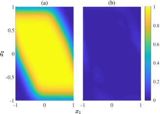
Figure 1: (a) Approximate safety probabilities computed using Algorithm 1 for a double integrator at $k=0$ for $N=3$. (b) Absolute error $|V_{0}^{\pi}(x)-\mkern 1.5mu\overline{\mkern-1.5muV\mkern-1.5mu}\mkern 1.5mu_{0}^{\pi}(x)|$ between the dynamic programming solution and Algorithm 1 at $k=0$ for $N=3$.

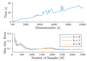
Figure 2: (top) System dimensionality [$n$] vs. average computation time [$s$] for an $n$-D stochastic integrator system. (bottom) Number of samples [$M$] vs. maximum absolute error $|V_{0}^{\pi}(x)-\mkern 1.5mu\overline{\mkern-1.5muV\mkern-1.5mu}\mkern 1.5mu_{0}^{\pi}(x)|$ for time steps $k=2$ to $k=0$ for $N=3$.

IV-B Clohessy-Wiltshire-Hill System

Lastly, we considered the more realistic example of spacecraft rendezvous and docking, in which a spacecraft must dock with another spacecraft while remaining within a line of sight cone. The Clohessey-Wiltshire-Hill dynamics,

$$\ddot{x}-3\omega x-2\omega\dot{y} =F_{x}/m_{d} \ddot{y}+2\omega\dot{x} =F_{y}/m_{d}$$ (36)

with state $\boldsymbol{z}=[x,y,\dot{x},\dot{y}]\in\mathcal{X}\subseteq\Re^{4}$, input $u=[F_{x},F_{y}]\in\mathcal{U}\subseteq\Re^{2}$, where $\mathcal{U}=[-0.1,0.1]\times[-0.1,0.1]$, and parameters $\omega$, $m_{d}$ can be written as a discrete-time LTI system $\boldsymbol{z}_{k+1}=A\boldsymbol{z}_{k}+Bu_{k}+\boldsymbol{w}_{k}$ with an additive Gaussian disturbance [3] with variance $\Sigma=\textnormal{diag}(1\times 10^{-4},1\times 10^{-4},5\times 10^{-8},5\times 10^{-8})$ such that $\boldsymbol{w}_{k}\sim\mathcal{N}(0,\Sigma)$. The target set and safe set are defined as in [3]:

$$\mathcal{T} =\{\boldsymbol{z}\in\Re^{4}:\begin{aligned} &|\boldsymbol{z}_{1}|\leq 0.1,-0.1<\boldsymbol{z}_{2}<0,\\ &|\boldsymbol{z}_{3}|\leq 0.01,|\boldsymbol{z}_{4}|\leq 0.01\}\end{aligned}$$ (37)

$$\mathcal{K} =\{\boldsymbol{z}\in\Re^{4}:|\boldsymbol{z}_{1}|<|\boldsymbol{z}_{2}|,|\boldsymbol{z}_{3}|\leq 0.05,|\boldsymbol{z}_{4}|\leq 0.05\}$$ (38)

We generate samples using [37] with a chance-affine controller.

Fig. 3(b) shows the approximate safety probabilities for time horizon $N=5$, with a precomputed safety controller from [36, 37]. The safety probabilities for the entire region were computed in 0.48 seconds (Table I), almost two orders of magnitude less than the chance constrained approach [36], which computes the set of initial conditions where the safety probability is above a certain threshold (0.8 in this case).

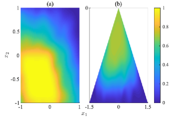
Figure 3: (a) Approximate safety probabilities computed using Algorithm 1 for a double integrator with a $\textnormal{Beta}(0.5,0.5)$ disturbance at $k=0$ for $N=1$. (b) Terminal-hitting safety probabilities for a CWH system with a Gaussian disturbance and a chance-affine controller at $k=0$ for $N=5$.

IV-C Sample Size and Parameter Tuning

The number of samples used to create the estimate $\bar{\mu}_{(x,u)}$ is the most significant computational bottleneck for Algorithm 1 and is generally $\mathcal{O}(M^{3})$. As the number of samples increases, the absolute error in the approximate safety probabilities decreases. However, methods have been developed recently to reduce the computational complexity [38, 39, 31] to $\mathcal{O}(M\log M)$. Additionally, for high-dimensional systems, the number of samples needed to fully characterize the system dynamics and disturbance increases as the system dimensionality increases, which is prohibitive for analysis over large regions of the state space. However, due to the sample-based nature of Algorithm 1, we can choose samples within a local region of interest in order to approximate the safety probabilities.

The kernel bandwidth parameter and the regularization parameter are tunable parameters which can affect the quality of the estimate obtained using Algorithm 1. A cross-validation scheme to empirically choose these parameters is presented in [30, Section 6].

V Conclusions & Future Work

We present a sample-based method to compute the stochastic reachability probability measure for Markov control systems with arbitrary disturbances that does not require a known model of the transition kernel. Our approach employs efficient computation associated with a reproducing kernel Hilbert space to approximate conditional distributions via simple matrix operations. The method is demonstrated on a 10,000-dimensional integrator as well as a realistic model of relative spacecraft motion. We plan to extend this to sample-based controller synthesis, with application to systems with autonomous and human elements.

References

- [1] S. Summers and J. Lygeros, “Verification of discrete time stochastic hybrid systems: A stochastic reach-avoid decision problem,” Automatica, vol. 46, no. 12, pp. 1951–1961, Dec. 2010.
- [2] A. Abate, M. Prandini, J. Lygeros, and S. Sastry, “Probabilistic reachability and safety for controlled discrete time stochastic hybrid systems,” Automatica, vol. 44, no. 11, pp. 2724–2734, November 2008.
- [3] K. Lesser, M. Oishi, and R. Erwin, “Stochastic reachability for control of spacecraft relative motion,” in IEEE Conf. Dec. & Ctrl., Dec 2013, pp. 4705–4712.
- [4] A. Vinod, V. Sivaramakrishnan, and M. Oishi, “Piecewise-affine approximation-based stochastic optimal control with Gaussian joint chance constraints,” in Amer. Ctl. Conf., 2019.
- [5] H. Sartipizadeh, A. Vinod, B. Acikmese, and M. Oishi, “Voronoi partition-based scenario reduction for fast sampling-based stochastic reachability computation of LTI systems,” Amer. Ctrl. Conf., pp. 37–44, 2018.
- [6] A. Vinod, B. HomChaudhuri, C. Hintz, A. Parikh, S. Buerger, M. Oishi, G. Brunson, S. Ahmad, and R. Fierro, “Multiple pursuer-based intercept via forward stochastic reachability,” in Amer. Ctrl. Conf., 2018, pp. 1559–1566.
- [7] A. Vinod, S. Rice, Y. Mao, M. Oishi, and B. Açıkmeşe, “Stochastic motion planning using successive convexification and probabilistic occupancy functions,” in IEEE Conf. Dec. & Ctrl., 2018, pp. 4425–4432.
- [8] A. Vinod and M. Oishi, “Scalable underapproximative verification of stochastic LTI systems using convexity and compactness,” in Hybrid Sys.: Comp. and Ctrl., 2018, pp. 1–10.
- [9] A. Vinod and M. Oishi, “Scalable underapproximation for the stochastic reach-avoid problem for high dimensional LTI systems using Fourier transforms,” IEEE Ctrl. Syst. Letters, vol. 1, no. 2, pp. 316–321, 2017.
- [10] N. Kariotoglou, S. Summers, T. Summers, M. Kamgarpour, and J. Lygeros, “Approximate dynamic programming for stochastic reachability,” in Euro. Ctrl. Conf., 2013, pp. 584–589.
- [11] G. Manganini, M. Pirotta, M. Restelli, L. Piroddi, and M. Prandini, “Policy search for the optimal control of Markov decision processes: A novel particle-based iterative scheme,” IEEE Trans. on Cybern., vol. 46, no. 11, pp. 2643–2655, 2015.
- [12] I. Mitchell, A. Bayen, and C. Tomlin, “A time-dependent Hamilton-Jacobi formulation of reachable sets for continuous dynamic games,” IEEE Trans. Autom. Ctrl., vol. 50, no. 7, pp. 947–957, 2005.
- [13] J. Fisac, M. Chen, C. Tomlin, and S. Sastry, “Reach-avoid problems with time-varying dynamics, targets and constraints,” in Hybrid Syst.: Comput. and Ctrl., 2015, pp. 11–20.
- [14] R. Bellman and S. Dreyfus, Applied Dynamic Programming. Princeton University Press, 1962.
- [15] B. Schölkopf and A. Smola, Learning with kernels: Support vector machines, regularization, optimization, and beyond. Cambridge, MA: MIT Press, 2002.
- [16] J. Shawe-Taylor and N. Cristianini, Kernel Methods for Pattern Analysis. New York, NY: Cambridge University Press, 2004.
- [17] N. Aronszajn, “Theory of reproducing kernels,” Trans. of the Amer. Math. Soc., vol. 68, no. 3, pp. 337–404, 1950.
- [18] S. Grünewälder, G. Lever, L. Baldassarre, M. Pontil, and A. Gretton, “Modelling transition dynamics in MDPs with RKHS embeddings,” in Int’l Conf. Mach. Learn., 2012, pp. 535–542.
- [19] L. Song, K. Fukumizu, and A. Gretton, “Kernel embeddings of conditional distributions: A unified kernel framework for nonparametric inference in graphical models,” IEEE Signal Process. Mag., vol. 30, pp. 98–111, Jul. 2013.
- [20] A. Smola, A. Gretton, L. Song, and B. Schölkopf, “A Hilbert space embedding for distributions,” in Int’l Conf. Algorithmic Learn. Theory, 2007, pp. 13–31.
- [21] G. Lever and R. Stafford, “Modelling policies in mdps in reproducing kernel hilbert space,” in Artif. Intell. and Stats., 2015, pp. 590–598.
- [22] Y. Nishiyama, A. Boularias, A. Gretton, and K. Fukumizu, “Hilbert space embeddings of POMDPs,” in Uncertainty Artif. Intell., 2012, pp. 644–653.
- [23] L. Song, J. Huang, A. Smola, and K. Fukumizu, “Hilbert space embeddings of conditional distributions with applications to dynamical systems,” in Int’l Conf. Mach. Learn., 2009, pp. 961–968.
- [24] P. Billingsley, Probability and Measure. John Wiley & Sons, 2012.
- [25] Y. Chow and H. Teicher, Probability Theory: Independence, Interchangeability, Martingales. Springer, 2012.
- [26] M. Puterman, Markov Decision Processes: Discrete Stochastic Dynamic Programming. John Wiley & Sons, 2014.
- [27] D. Bertsekas and S. Shreve, Stochastic optimal control: The discrete-time case. Athena Scientific Publ., 1996.
- [28] I. Steinwart and A. Christmann, Support vector machines. Springer, 2008.
- [29] A. Berlinet and C. Thomas-Agnan, Reproducing Kernel Hilbert Spaces in Probability and Statistics. Springer, 2011.
- [30] C. Micchelli and M. Pontil, “On learning vector-valued functions,” Neural Comput., vol. 17, no. 1, pp. 177–204, 2005.
- [31] S. Grünewälder, G. Lever, L. Baldassarre, S. Patterson, A. Gretton, and M. Pontil, “Conditional mean embeddings as regressors,” in Int’l Conf. Mach. Learn., 2012, pp. 1823–1830.
- [32] B. Sriperumbudur, A. Gretton, K. Fukumizu, B. Schölkopf, and G. Lanckriet, “Hilbert space embeddings and metrics on probability measures,” J. Mach. Learn. Res., vol. 11, pp. 1517–1561, Aug. 2010.
- [33] A. Gretton, K. Borgwardt, M. Rasch, B. Schölkopf, and A. Smola, “A kernel method for the two-sample-problem,” in Adv. Neural Inf. Proc. Sys., 2007, pp. 513–520.
- [34] A. Gretton, K. Borgwardt, M. Rasch, B. Schölkopf, and A. Smola, “A kernel two-sample test,” J. Mach. Learn. Res., vol. 13, pp. 723–773, 2012.
- [35] K. Fukumizu, A. Gretton, X. Sun, and B. Schölkopf, “Kernel measures of conditional dependence,” in Adv. Neural Inf. Proc. Sys., 2008, pp. 489–496.
- [36] A. Vinod and M. Oishi, “Affine controller synthesis for stochastic reachability via difference of convex programming,” in IEEE Conf. Dec. & Ctrl. (to appear), 2019.
- [37] A. Vinod, J. Gleason, and M. Oishi, “SReachTools: A Matlab stochastic reachability toolbox,” in Hybrid Sys: Comp. & Ctrl., 2019, pp. 33–38.
- [38] A. Rahimi and B. Recht, “Random features for large-scale kernel machines,” in Adv. Neural Inf. Process. Syst., 2008, pp. 1177–1184.
- [39] Q. Le, T. Sarlós, and A. Smola, “Fastfood–approximating kernel expansions in loglinear time,” in Int’l Conf. Mach. Learn., 2013.