Monotonic and nonmonotonic immune responses in viral infection systems

Abstract

In this paper, we study two-dimensional, three-dimensional monotonic and nonmonotonic immune responses in viral infection systems. Our results show that the viral infection systems with monotonic immune response has no bistability appear. However, the systems with nonmonotonic immune response has bistability appear under some conditions. For immune intensity, we got two important thresholds, post-treatment control threshold and elite control threshold. When immune intensity is less than post-treatment control threshold, the virus will be rebound. The virus will be under control when immune intensity is larger than elite control threshold. While between the two thresholds is a bistable interval. When immune intensity is in the bistable interval, the system can have bistability appear. Select the rate of immune cells stimulated by the viruses as a bifurcation parameter for nonmonotonic immune responses, we prove the system exhibits saddle-node bifurcation and transcritical bifurcation.

1 Introduction

During the process of viral infection, the host is induced which is initially rapid and nonspecific (natural killer cells, macrophage cells, etc.) and then delayed and specific (cytotoxic T lymphocyte cells, antibody cell). But in most virus infections, cytotoxic T lymphocyte (CTL) cells which attack infected cells and antibody cells which attack viruses, play a critical part in antiviral defense. Some researchers have studied some models about virus dynamics within-host and immune response, [1, 2, 3, 4, 5] and others don’t contain the immune responses. [6, 7, 8, 9, 10, 11]

In order to investigate the role of the population dynamics of viral infection with CTL response, Nowak and Bangham (see e.g. Refs [12]) constructed a mathematical model describing the basic dynamics of the interaction between activated CD4⁺ T cells, $x(t)$, infected CD4⁺ T cells, $y(t)$, viruses, $v(t)$ and immune cells, $z(t)$.

$$\left\{\begin{array}[]{l l}\frac{dx}{dt}=s-dx-(1-\epsilon)\beta xy,\\ \frac{dy}{dt}=(1-\epsilon)\beta xy-ay-pyz,\\ \frac{dz}{dt}=f(y)z-bz,\end{array}\right.$$

where $f(y)$ is a continuously differentiable function defined on $[0,+\infty)$ and satisfies

$$f^{{}^{\prime}}(y)>0,~{}f(0)=0~{}\mbox{and}~{}f(y)\leq My~{}\mbox{for some positive parameter }M.$$

For example, $f(y)=cy$ or $f(y)=\frac{cy}{1+\alpha y}$ is the common monotonic immune response in viral infection systems. [15, 16] In 1968, Andrews (see e.g. Refs [13]) suggested Monod-Haldane function

$$f(y)=\frac{cy}{\alpha+\gamma y+y^{2}},$$

then, Sokol and Howell (see e.g. Refs [14]) proposed a simplified Monod-Haldane function

$$f(y)=\frac{cy}{\alpha+y^{2}},$$

as nonmonotonic functions in chemostat systems. The nonmonotonic functions are also discussed in predator-prey system. [17, 18, 19] Wang et al (see e.g. Refs [20]) proposed oxidative stress in a HIV infection model and the immune function is a Monod-Haldane function. Thus we chose $\frac{cyz}{\alpha+\gamma y+y^{2}}$ as the nonmonotonic immune response in the following system.

$$\left\{\begin{array}[]{l l}\frac{dx}{dt}=s-dx-(1-\epsilon)\beta xy=g_{1},\\ \frac{dy}{dt}=(1-\epsilon)\beta xy-ay-pyz=g_{2},\\ \frac{dz}{dt}=\frac{cyz}{\alpha+\gamma y+y^{2}}-bz=g_{3}.\end{array}\right.$$

Activated CD4⁺ T cells are generated at a rate $s$, die at a rate $d$, and become infected CD4⁺ T cells at a rate $(1-\epsilon)\beta xy$. Infected CD4⁺ T cells die at a rate $a$ and are killed by immune cells at a rate $pyz$. $\frac{cyz}{\alpha+\gamma y+y^{2}}$ represents the immune cells stimulated by the viruses and die at a rate $b$. All the parameters are positive.

The rest of this paper is organized as follows. The viral infection system with monotonic immune response is carried out in section 2. The stability analysis, bifurcation analysis and numerical simulations of nonmonotonic immune response is carried out in Section 3. In section 4, we analyze the 2D-viral infection system with monotonic immune response. In section 5, we analyze the stability and bifurcation of the 2D-viral infection system with monotonic immune response and carry out numerical simulations. In section 6, we conclude the paper with discussions.

2 Viral infection system with monotonic immune response

System (1.1) always has an uninfected steady equilibrium $E^{(1)}_{0}=(x^{(1)}_{0},0,0)$, and if $\mathcal{R}^{(1)}_{0}>1>\mathcal{R}^{(1)}_{*}$, system (1.1) also has an immune-free equilibrium $E^{(1)}_{1}=(x^{(1)}_{1},y^{(1)}_{1},0)$; If $\mathcal{R}^{(1)}_{0}>\mathcal{R}^{(1)}_{*}>1$ system (1.1) has three equilibria $E^{(1)}_{0}$, $E^{(1)}_{1}$ and $E^{(1)}_{*}=(x^{(1)}_{*},y^{(1)}_{*},z^{(1)}_{*})$, where

$$\begin{array}[]{ll}x^{(1)}_{0}=\frac{s}{d},\\ \vspace{2\jot}x^{(1)}_{1}=\frac{a}{\beta(1-\epsilon)},\\ \vspace{2\jot}y^{(1)}_{1}=\frac{d(R^{(1)}_{0}-1)}{\beta(1-\epsilon)},\\ \vspace{2\jot}x^{(1)}_{*}=\frac{s}{d+(1-\epsilon)\beta y^{(1)}_{*}},\\ \vspace{2\jot}\displaystyle y^{(1)}_{*}=f^{-1}(b),\\ \vspace{2\jot}\displaystyle z^{(1)}_{*}=\frac{a(R^{(1)}_{*}-1)}{p}.\end{array}$$

The basic reproductive number is given as

$$\mathcal{R}^{(1)}_{0}=(1-\epsilon)\beta\frac{s}{d}\frac{1}{a}1=\frac{s\beta(1-\epsilon)}{ad}.$$

Because $(1-\epsilon)\beta\frac{s}{d}\frac{1}{a}$ is the basic reproductive number of the model with the bilinear incidence $\beta xy$, ${R}^{(1)}_{0}$ gives the basic reproductive number of system (1.1) with the constant function response.

The basic immune reproductive number is

$$\mathcal{R}^{(1)}_{*}=\frac{s\beta(1-\epsilon)}{ad+a\beta(1-\epsilon)y^{(1)}_{*}}.$$

This ratio describes the average number of newly infected cells generated form on infected cells at the beginning of the infectious process.

Let $\tilde{E}$ be any arbitrary equilibrium of system (1.1). The Jacobian matrix associated with the system is

$$J_{1}=\left[\begin{array}[]{cccc}-d-\beta(1-\epsilon)y&-\beta(1-\epsilon)x&0\\ \beta(1-\epsilon)y&\beta(1-\epsilon)x-a-pz&-py\\ 0&f^{{}^{\prime}}(y)z&f(y)-b\\ \end{array}\right].$$

The characteristic equation of the linearized system of (1.1) at $\tilde{E}$ is given by $\left|\lambda I-J_{1}\right|=0.$

Lemma 2.1 $\mathcal{R}^{(1)}_{*}<1\Leftrightarrow y^{(1)}_{1}<y^{(1)}_{*}$.

Proof.

$$\begin{array}[]{lll}\mathcal{R}^{(1)}_{*}<1&\Leftrightarrow&\frac{(1-\epsilon)\beta s}{ad+(1-\epsilon)a\beta y^{(1)}_{*}}<1,\\ &\Leftrightarrow&\mathcal{R}^{(1)}_{0}<1+\frac{(1-\epsilon)\beta y^{(1)}_{*}}{d}\\ &\Leftrightarrow&\frac{d(\mathcal{R}^{(1)}_{0}-1)}{\beta(1-\epsilon)}<y^{(1)}_{*}\\ &\Leftrightarrow&y^{(1)}_{1}<y^{(1)}_{*}.\end{array}$$

Theorem 2.1   If $\mathcal{R}^{(1)}_{0}<1$, then the uninfected equilibrium $E^{(1)}_{0}$ of system (1.1) is not only locally asymptotically stable, but also global asymptotically stable. If $\mathcal{R}^{(1)}_{0}>1$, then the uninfected equilibrium $E^{(1)}_{0}$ of system (1.1) is unstable.

Proof. The characteristic equation of the linearized system of system (1.1) at $E^{(1)}_{0}$ is

$$(\lambda+b)(\lambda+d)(\lambda+a-(1-\epsilon)\beta x^{(1)}_{0})=0.$$

Obviously, the characteristic roots $-d$, $-b$, and $a(\mathcal{R}^{(1)}_{0}-1)$ are negative for $\mathcal{R}^{(1)}_{0}<1$. Hence $E^{(1)}_{0}$ is locally asymptotically stable. If $\mathcal{R}^{(1)}_{0}>1$, then $a(\mathcal{R}^{(1)}_{0}-1)>0$, thus, the uninfected equilibrium $E^{(1)}_{0}$ of system (1.1) is unstable.

Consider the Lyapunov function

$$V_{0}=\frac{1}{2}(x-x^{(1)}_{0})^{2}+x^{(1)}_{0}y+\frac{px^{(1)}_{0}}{M}z.$$

Differentiating $V_{0}$ along solutions of system (1.1) yields

$$\begin{array}[]{lll}\begin{split}\displaystyle\dot{V_{0}}|_{(1.1)}&=\displaystyle(x-x^{(1)}_{0})[s-dx-(1-\epsilon)\beta xy]+x^{(1)}_{0}[(1-\epsilon)\beta xy-ay-pyz]\\ &\displaystyle+\frac{px^{(1)}_{0}}{M}[f(y)z-bz]\vspace{0.2cm}\\ &=\displaystyle(x-x^{(1)}_{0})[dx^{(1)}_{0}-dx-(1-\epsilon)\beta xy]+x^{(1)}_{0}[(1-\epsilon)\beta xy-ay-pyz]\\ &\displaystyle+\frac{px^{(1)}_{0}}{M}f(y)z-\frac{px^{(1)}_{0}}{M}bz\vspace{0.2cm}\\ &\leq-d(x-x^{(1)}_{0})^{2}-(1-\epsilon)\beta x^{2}y+2(1-\epsilon)\beta x^{(1)}_{0}xy-ax^{(1)}_{0}y-\frac{px^{(1)}_{0}}{M}bz\\ &=-[d+(1-\epsilon)\beta y](x-x^{(1)}_{0})^{2}-ax^{(1)}_{0}y(1-R^{(1)}_{0})-\frac{px^{(1)}_{0}}{M}bz.\end{split}\end{array}$$

If $R^{(1)}_{0}<1$, then $\dot{V_{0}}|_{(1.1)}\leq 0$. Furthermore,

$$W_{0}=\{(x,y,z)|\dot{V_{0}}=0\}=\{(x,y,z)|x=x^{(1)}_{0},y=0,z=0\}.$$

Therefore, the largest invariant set contained in $W_{0}$ is $E_{0}^{(1)}$. By $LaSalle^{\prime}s$ invariance principle, [22, 23] we infer that all the solutions of system (1.1) that start in $R^{3}>0$ limit to $E_{0}^{(1)}$. Besides, $E_{0}^{(1)}$ is Lyapunov stable, prove that $E_{0}^{(1)}$ is globally asymptotically stable. Theorem 2.1 is proved.

Theorem 2.2   If $\mathcal{R}^{(1)}_{0}>1>\mathcal{R}^{(1)}_{*}$, then the immune-free equilibrium $E^{(1)}_{1}$ of system (1.1) is locally asymptotically stable. $E^{(1)}_{1}$ is unstable for $\mathcal{R}^{(1)}_{*}>1$.

Proof. The characteristic equation of the linearized system of (1.1) at $E^{(1)}_{1}$ is given by

$$[\lambda-(f(y^{(1)}_{1})-b)][\lambda^{2}+a^{(1)}_{1}\lambda+a^{(1)}_{2}]=0,$$

where

$$\begin{array}[]{lll}a^{(1)}_{1}&=&d+(1-\epsilon)\beta y^{(1)}_{1},\\ a^{(1)}_{2}&=&(1-\epsilon)^{2}\beta^{2}x^{(1)}_{1}y^{(1)}_{1}.\end{array}$$

By (1.2), $f^{{}^{\prime}}(y)>0$ for $[0,+\infty)$ and $f(y^{(1)}_{*})=b$, we deduce the eigenvalue $\lambda=f(y^{(1)}_{1})-b<0$ for $\mathcal{R}^{(1)}_{0}>1>{R}^{(1)}_{*}$, and $\lambda=f(y^{(1)}_{1})-b>0$ for $\mathcal{R}^{(1)}_{*}>1$. $a^{(1)}_{1}>0$ and $a^{(1)}_{2}>0$ inducing, the other eigenvalues are negative. Thus, the immune-free equilibrium $E^{(1)}_{1}$ of system (1.1) is locally asymptotically stable for $\mathcal{R}^{(1)}_{0}>1>\mathcal{R}^{(1)}_{*}$ and $E^{(1)}_{1}$ is unstable for ${R}^{(1)}_{*}>1$.

Theorem 2.3   If $\mathcal{R}^{(1)}_{*}>1$, then the positive equilibrium $E^{(1)}_{*}$ of system (1.1) is locally asymptotically stable.

Proof. The characteristic equation of the linearized system of (1.1) at $E^{(1)}_{*}$ is given by

$$\lambda^{3}+b^{(1)}_{1}\lambda^{2}+b^{(1)}_{2}\lambda+b^{(1)}_{3}=0,$$

where

$$\begin{array}[]{lll}b^{(1)}_{1}&=&d+(1-\epsilon)\beta y^{(1)}_{*},\\ b^{(1)}_{2}&=&py^{(1)}_{*}z^{(1)}_{*}f^{{}^{\prime}}(y^{(1)}_{*})+(1-\epsilon)^{2}\beta^{2}x^{(1)}_{*}y^{(1)}_{*},\\ b^{(1)}_{3}&=&py^{(1)}_{*}z^{(1)}_{*}f^{{}^{\prime}}(y^{(1)}_{*})[d+(1-\epsilon)\beta y^{(1)}_{*}].\end{array}$$

It is easy to see, $b^{(1)}_{i}>0(i=1,2,3)$ and $b^{(1)}_{1}b^{(1)}_{2}-b^{(1)}_{3}=(1-\epsilon)^{2}\beta^{2}x^{(1)}_{*}y^{(1)}_{*}[d+(1-\epsilon)\beta y^{(1)}_{*}]>0$. By Routh-Hurartz Criterion, we know the positive equilibrium $E^{(1)}_{*}$ of system (1.1) is locally asymptotically stable for $\mathcal{R}^{(1)}_{*}>1$.

By Theorem 2.1$\sim$2.3, we can get following result:

Remark 2.1 Viral infection system with monotonic immune response has no bistability appear.

3 Viral infection system with nonmonotonic immune response

3.1 Equilibria and thresholds

In this section, we discuss the viral infection system with nonmonotonic immune response (1.3) and always assume $\gamma>2\sqrt{\alpha}$. We denote basic reproductive number ${R}^{(2)}_{0}=\frac{s\beta(1-\epsilon)}{ad}$, which is equivalent to ${R}^{(1)}_{0}$.

(i) If $\mathcal{R}^{(2)}_{0}<1$, system (1.3) only exists an uninfected equilibrium $E^{(2)}_{0}=(x^{(2)}_{0},0,0)$ , where $x^{(2)}_{0}=\frac{s}{d}$ .

(ii) If $\mathcal{R}^{(2)}_{0}>1$, system (1.3) also has an immune-free equilibrium $E^{(2)}_{1}=(x^{(2)}_{1},y^{(2)}_{1},0),$ where $x^{(2)}_{1}=\frac{a}{\beta(1-\epsilon)},y^{(2)}_{1}=\frac{d({R}^{(2)}_{0}-1)}{\beta(1-\epsilon)}.$

Solving equation $\frac{cy}{\alpha+\gamma y+y^{2}}-b=0$, one get two positive roots, $c_{1}=\gamma b-2b\sqrt{\alpha}$ and $c_{2}=\gamma b+2b\sqrt{\alpha}$ , then the existence conditions of positive equilibria as following:

(iii) If $\mathcal{R}_{*}^{1-}>1$ and $c>c_{2},$ system (1.3) has an immune equilibrium $E_{*}^{2-}=(x_{*}^{2-},y_{*}^{2-},z_{*}^{2-})$; If $\mathcal{R}_{*}^{1+}>1$ and $c>c_{2},$ system (1.3) also has an immune equilibrium $E_{*}^{2+}=(x_{*}^{2+},y_{*}^{2+},z_{*}^{2+}).$ Here $\mathcal{R}_{*}^{1\pm}=\frac{(1-\epsilon)\beta s-ad}{(1-\epsilon)\beta ay_{*}^{2\pm}},x_{*}^{2\pm}=\frac{s}{(1-\epsilon)\beta y_{*}^{2\pm}+d},y_{*}^{2\pm}=\frac{-B\pm\sqrt{B^{2}-4\alpha b^{2}}}{2b},z_{*}^{2\pm}=\frac{(1-\epsilon)\beta ay_{*}^{2\pm}(\mathcal{R}_{*}^{1\pm}-1)}{p[(1-\epsilon)\beta y_{*}^{2\pm}+d]},B=\gamma b-c.$

We denote post-treatment control threshold $P_{I}$ (see e.g. Refs [21])

$$c_{2}=\gamma b+2b\sqrt{\alpha}.$$

Denote

$$c^{*}_{1}=\gamma b+\frac{2bd(\mathcal{R}^{(2)}_{0}-1)}{\beta(1-\epsilon)},$$

$$c^{**}_{1}=\gamma b+\frac{bd(\mathcal{R}^{(2)}_{0}-1)}{\beta(1-\epsilon)}+\frac{\alpha\beta b(1-\epsilon)}{d(\mathcal{R}^{(2)}_{0}-1)}.$$

We call $c^{**}_{1}$ the elite control threshold $E_{1}$, [21] which means the virus will be under control when the immune intensity $c$ is larger than $c^{**}_{1}$.
Denote another threshold

$$\mathcal{R}^{(1)}_{c}=1+\frac{\beta(1-\epsilon)}{d}\sqrt{\alpha}.$$

For the positive parameters in model (1.3), we have the following lemmas.

Lemma 3.1 $\mathcal{R}^{(2)}_{0}>\mathcal{R}^{(1)}_{c}>1\Leftrightarrow c^{*}_{1}>c^{**}_{1}.$

Proof.

$$\begin{array}[]{lll}c^{*}_{1}>c^{**}_{1}&\Leftrightarrow&\frac{bd(\mathcal{R}^{(2)}_{0}-1)}{\beta(1-\epsilon)}>\frac{\alpha\beta b(1-\epsilon)}{d(\mathcal{R}^{(2)}_{0}-1)},\\ &\Leftrightarrow&\mathcal{R}^{(2)}_{0}>\mathcal{R}^{(1)}_{c}.\end{array}$$

Lemma 3.2 (i) $\mathcal{R}^{(2)}_{0}>\mathcal{R}^{(1)}_{c}>1\Leftrightarrow c^{*}_{1}>c_{2}$; (ii) $1<\mathcal{R}^{(2)}_{0}<\mathcal{R}^{(1)}_{c}\Leftrightarrow c^{*}_{1}<c_{2}.$

Proof.

$$\begin{array}[]{lll}c^{*}_{1}>c_{2}&\Leftrightarrow&\frac{2bd(\mathcal{R}^{(2)}_{0}-1)}{\beta(1-\epsilon)}>2b\sqrt{\alpha},\\ &\Leftrightarrow&\mathcal{R}^{(2)}_{0}>R^{(1)}_{c}.\end{array}$$

$$\begin{array}[]{lll}c^{*}_{1}<c_{2}&\Leftrightarrow&\frac{2bd({R}^{(2)}_{0}-1)}{\beta(1-\epsilon)}<2b\sqrt{\alpha},\\ &\Leftrightarrow&\mathcal{R}^{(2)}_{0}<R^{(1)}_{c}.\end{array}$$

Lemma 3.3 (i) Assume $1<\mathcal{R}^{(2)}_{0}<\mathcal{R}^{(1)}_{c}.$ If $\mathcal{R}_{*}^{1-}>1$, then $c>c^{**}_{1}$; (ii) Assume $\mathcal{R}^{(2)}_{0}>\mathcal{R}^{(1)}_{c}>1.$ If $\mathcal{R}_{*}^{1-}>1$, then $c>c_{2}$.

Proof.

$$\begin{array}[]{lll}\mathcal{R}_{*}^{1-}>1&\Leftrightarrow&\frac{\beta s(1-\epsilon)-ad}{\beta a(1-\epsilon)y_{*}^{2-}}>1,\\ &\Leftrightarrow&\sqrt{(\gamma b-c)^{2}-4\alpha b^{2}}>c-c^{*}_{1}.\end{array}$$

If $c<c^{*}_{1}$ and one of conditions $c<c_{1}$ or $c>c_{2}$ is correct, then $\mathcal{R}_{*}^{1-}$ is always larger than one. If $c>c^{*}_{1}$, solving $\sqrt{(\gamma b-c)^{2}-4\alpha b^{2}}>c-c^{*}_{1}$, we have $c>c^{**}_{1}.$ Thus,

(i) If $1<\mathcal{R}^{(2)}_{0}<\mathcal{R}^{(1)}_{c}$, then $c^{*}_{1}<c_{2}$. From $\mathcal{R}_{*}^{1-}>1$, we have $c>c^{**}_{1}.$

(ii) If $\mathcal{R}^{(2)}_{0}>\mathcal{R}^{(1)}_{c}>1$, then $c^{*}_{1}>c_{2}$. From $\mathcal{R}_{*}^{1-}>1$, we have $c>c_{2}.$

Lemma 3.4 (i) If $1<\mathcal{R}^{(2)}_{0}<\mathcal{R}^{(1)}_{c},$ then $\mathcal{R}_{*}^{1+}>1$ has no solution; (ii) Assume $\mathcal{R}^{(2)}_{0}>\mathcal{R}^{(1)}_{c}>1$. If $\mathcal{R}_{*}^{1+}>1$, then $c_{2}<c<c^{**}_{1}$.

Proof.

$$\begin{array}[]{lll}\mathcal{R}_{*}^{1+}>1&\Leftrightarrow&\frac{\beta s(1-\epsilon)-ad}{\beta a(1-\epsilon)y_{*}^{2+}}>1,\\ &\Leftrightarrow&c^{*}_{1}-c>\sqrt{(\gamma b-c)^{2}-4\alpha b^{2}}.\end{array}$$

(i) If $1<{R}^{(2)}_{0}<R^{(1)}_{c},$ then $c^{*}_{1}<c_{2}$. Thus $\mathcal{R}_{*}^{1+}>1$ has no solution. (ii) If $\mathcal{R}^{(2)}_{0}>\mathcal{R}^{(1)}_{c}>1$, then $c^{*}_{1}>c_{2}$. Solving $\mathcal{R}_{*}^{1+}>1$, we have $c_{2}<c<c^{**}_{1}$.

By Lemma 3.1 $\sim$ Lemma 3.4 and summing up the above analysis we obtain the existing results of equilibria of system (1.3).

Theorem 3.1 (i) System (1.3) always exists an uninfected equilibrium $E^{(2)}_{0};$

(ii) If $\mathcal{R}^{(2)}_{0}>1$, system (1.3) also has an immune-free equilibrium $E^{(2)}_{1};$

(iii) If $1<\mathcal{R}^{(2)}_{0}<\mathcal{R}^{(1)}_{c}$ and $c>c^{**}_{1},$ system (1.3) also has one positive equilibrium $E_{*}^{2-};$

(iv) If $\mathcal{R}^{(2)}_{0}>\mathcal{R}^{(1)}_{c}>1$ and $c_{2}<c<c^{**}_{1}$, system (1.3) has two positive equilibria $E_{*}^{2+}$ and $E_{*}^{2-}$. While $\mathcal{R}^{(2)}_{0}>\mathcal{R}^{(1)}_{c}$ and $c>c^{**}_{1}$, system (1.3) only has one positive equilibrium $E_{*}^{2-}$;

The summary results of the existence for positive equilibria can be seen in Table 1 and Table 2.

3.2 Stability analysis

Let $\tilde{E}$ be any arbitrary equilibrium of system (1.3). The Jacobian matrix associated with the system is

$$J_{2}=\left[\begin{array}[]{cccc}-d-\beta(1-\epsilon)y&-\beta(1-\epsilon)x&0\\ \beta(1-\epsilon)y&\beta(1-\epsilon)x-a-pz&-py\\ 0&\frac{c\alpha z-czy^{2}}{(\alpha+\gamma y+y^{2})^{2}}&\frac{cy}{\alpha+\gamma y+y^{2}}-b\\ \end{array}\right].$$

The characteristic equation of the linearized system of (1.3) at $\tilde{E}$ is given by $\left|\lambda I-J_{2}\right|=0.$

Theorem 3.2   If $\mathcal{R}^{(2)}_{0}<1$, then the uninfected equilibrium $E^{(2)}_{0}$ of system (1.3) is not only locally asymptotically stable, but also global asymptotically stable.

Proof. The characteristic roots of the linearized system of (1.3) at $E^{(2)}_{0}$ is given by $\lambda_{1}=-d$, $\lambda_{2}=-b$ and $\lambda_{3}=\frac{\mathcal{R}^{(2)}_{0}-1}{a}.$ So we can get $\mathcal{R}^{(2)}_{0}<1$ , the uninfected equilibrium $E^{(2)}_{0}$ is locally asymptotically stable.

Consider the Lyapunov function

$$V_{1}=\frac{1}{2}(x-x^{(2)}_{0})^{2}+x^{(2)}_{0}y+\frac{\alpha px^{(2)}_{0}}{c}z.$$

Differentiating $V_{1}$ along solutions of system (1.3) yields

$$\begin{array}[]{lll}\begin{split}\displaystyle\dot{V_{1}}|_{(1.3)}&=\displaystyle(x-x^{(2)}_{0})[s-dx-(1-\epsilon)\beta xy]+x^{(2)}_{0}[(1-\epsilon)\beta xy-ay-pyz]\\ &\displaystyle+\frac{\alpha px^{(2)}_{0}}{c}[\frac{cyz}{\alpha+\gamma y+y^{2}}-bz]\vspace{0.2cm}\\ &=\displaystyle(x-x^{(2)}_{0})[dx^{(2)}_{0}-dx-(1-\epsilon)\beta xy]+x^{(2)}_{0}[(1-\epsilon)\beta xy-ay-pyz]\\ &\displaystyle+\frac{\alpha px^{(2)}_{0}yz}{\alpha+\gamma y+y^{2}}-\frac{\alpha bpx^{(2)}_{0}}{c}z\vspace{0.2cm}\\ &\leq-d(x-x^{(2)}_{0})^{2}-(1-\epsilon)\beta x^{2}y+2(1-\epsilon)\beta x^{(2)}_{0}xy-ax^{(2)}_{0}y-\frac{\alpha bpx^{(2)}_{0}}{c}z\\ &=-[d+(1-\epsilon)\beta y](x-x^{(2)}_{0})^{2}-ax^{(2)}_{0}y(1-R^{(2)}_{0})-\frac{\alpha bpx^{(2)}_{0}}{c}z.\end{split}\end{array}$$

If $R^{(2)}_{0}<1$, then $\dot{V_{1}}|_{(1.3)}\leq 0$.

Furthermore,

$$W_{1}=\{(x,y,z)|\dot{V_{1}}=0\}=\{(x,y,z)|x=x^{(2)}_{0},y=0,z=0\}.$$

Therefore, the largest invariant set contained in $W_{1}$ is $E_{0}^{(2)}$. By $LaSalle^{\prime}s$ invariance principle, [22, 23] we infer that all the solutions of system (1.3) that start in $R^{3}>0$ limit to $E_{0}^{(2)}$. Besides, $E_{0}^{(2)}$ is Lyapunov stable, prove that $E_{0}^{(2)}$ is globally asymptotically stable. Theorem 3.2 is proved.

Theorem 3.3 Suppose $\mathcal{R}^{(2)}_{0}>1$. When $0<c<c^{**}_{1},$ $E^{(2)}_{1}$ is locally asymptotically stable. When $c>c^{**}_{1},$ $E^{(2)}_{1}$ is unstable.

Proof. The characteristic equation of the linearized system of (1.3) at $E^{(2)}_{1}$ is given by $[\lambda-(\frac{cy^{(2)}_{1}}{\alpha+\gamma y^{(2)}_{1}+{(y^{(2)}_{1}})^{2}}-b)][\lambda^{2}+a^{(2)}_{1}\lambda+a^{(2)}_{2}]=0$,
where

$$\begin{array}[]{lll}a^{(2)}_{1}&=&(1-\epsilon)\beta y^{(2)}_{1}+d>0,\\ a^{(2)}_{2}&=&(1-\epsilon)^{2}\beta^{2}x^{(2)}_{1}y^{(2)}_{1}>0.\end{array}$$

Another eigenvalue

$$\begin{array}[]{lll}\lambda=\frac{cy^{(2)}_{1}}{\alpha+\gamma y^{(2)}_{1}+{(y^{(2)}_{1}})^{2}}-b<0&\Leftrightarrow&c<c^{**}_{1}.\end{array}$$

In summary, if $0<c<c^{**}_{1},$ then $\lambda<0.$ Therefore, by Routh-Hurartz criterion, we know under the assumption of $\mathcal{R}^{(2)}_{0}>1$. If $0<c<c^{**}_{1},$ the equilibrium $E^{(2)}_{1}$ of system (1.3) is locally asymptotically stable. If $c>c^{**}_{1},$ $E^{(2)}_{1}$ is unstable.

Theorem 3.4 (i) If   ($\mathbf{A.1}$)    $1<\mathcal{R}^{(2)}_{0}<\mathcal{R}^{(1)}_{c}$ and $c>c^{**}_{1}$, or

($\mathbf{A.2}$)    $\mathcal{R}^{(2)}_{0}>\mathcal{R}^{(1)}_{c}$ and $c>c_{2}$,
system (1.3) has an immune equilibrium $E_{*}^{2-},$ which is a stable node.

(ii) If $\mathcal{R}^{(2)}_{0}>\mathcal{R}^{(1)}_{c}$ and $c_{2}<c<c^{**}_{1}$, system (1.3) also has an immune equilibrium $E_{*}^{2+},$ which is an unstable saddle.

Proof. Denote $E_{*}^{(2)}=(x_{*}^{(2)},y_{*}^{(2)},z_{*}^{(2)})$ as an arbitrary positive equilibrium of system (1.3). The characteristic equation of the linearized system of (1.3) at the arbitrary positive equilibrium $E_{*}^{(2)}$ is given by

$$\lambda^{3}+b^{(2)}_{1}\lambda^{2}+b^{(2)}_{2}\lambda+b^{(2)}_{3}=0,$$

where

$$\begin{array}[]{lll}b^{(2)}_{1}&=&(1-\epsilon)\beta y_{*}^{(2)}+d>0,\\ b^{(2)}_{2}&=&(1-\epsilon)^{2}\beta^{2}x_{*}^{(2)}y_{*}^{(2)}+cpy_{*}^{(2)}z_{*}^{(2)}\frac{\alpha-(y_{*}^{(2)})^{2}}{(\alpha+\gamma y_{*}^{(2)}+(y_{*}^{(2)})^{2})^{2}},\\ b^{(2)}_{3}&=&cpy_{*}^{(2)}z_{*}^{(2)}[(1-\epsilon)\beta y_{*}^{(2)}+d]\frac{\alpha-(y_{*}^{(2)})^{2}}{(\alpha+\gamma y_{*}^{(2)}+(y_{*}^{(2)})^{2})^{2}},\end{array}$$

and

$$b^{(2)}_{1}b^{(2)}_{2}-b^{(2)}_{3}=[(1-\epsilon)\beta y_{*}^{(2)}+d](1-\epsilon)^{2}\beta^{2}x_{*}^{(2)}y_{*}^{(2)}>0.$$

For equilibrium $E_{*}^{2-},$

$$\begin{array}[]{lll}\alpha-(y_{*}^{2-})^{2}>0&\Leftrightarrow&\frac{-B-\sqrt{B^{2}-4\alpha b^{2}}}{2b}<\sqrt{\alpha},\\ &\Leftrightarrow&c>c_{2}.\end{array}$$

If $c>c_{2}$, we can get $b^{(2)}_{2}>0$ and $b^{(2)}_{3}>0$, by Routh-Hurartz Criterion, we know in this case the positive equilibrium $E_{*}^{2-}$ is a stable node.

For equilibrium $E_{*}^{2+},$

$$\begin{array}[]{lll}\alpha-(y_{*}^{2+})^{2}<0&\Leftrightarrow&\frac{-B+\sqrt{B^{2}-4\alpha b^{2}}}{2b}>\sqrt{\alpha},\\ &\Leftrightarrow&\sqrt{B^{2}-4\alpha b^{2}}>B+2b\sqrt{\alpha}.\end{array}$$

When $c_{2}<c<c^{**}_{1}$, then $b^{(2)}_{3}<0$, so the immune equilibrium $E_{*}^{2+}$ is an unstable saddle.

3.3 Saddle-node bifurcation

If $\mathcal{R}^{(2)}_{0}>\mathcal{R}^{(1)}_{c}>1$ and $c^{2}-2\gamma bc+\gamma^{2}b^{2}-4\alpha b^{2}=0$, the immune equilibrium $E_{*}^{2+}$ and $E_{*}^{2-}$ coincide with each other. Then system has the unique interior equilibrium $E_{*}^{(2)}=(x_{*}^{(2)},y_{*}^{(2)},z_{*}^{(2)})=(\frac{s}{(1-\epsilon)\beta\alpha+d},\sqrt{\alpha},\frac{1}{p}(\frac{(1-\epsilon)\beta s}{(1-\epsilon)\beta\alpha+d}-a)$. If $c<c^{[sn]}$, there is no positive equilibrium and there is two positive equilibria. Thus, system (1.3) will be a saddle-node bifurcation when $c$ crosses the bifurcation value $c^{[sn]}$, where $c^{[sn]}=\gamma b+2b\sqrt{\alpha}$.

Theorem 3.5 If $\mathcal{R}^{(2)}_{0}>\mathcal{R}^{(1)}_{c}>1$ and $c=c^{[sn]}$, system (1.3) undergoes a saddle-node bifurcation.

Proof. We use Sotomayor’s theorem [26, 27, 28] to prove system (1.3) undergoes a saddle-node bifurcation at $c=c^{[sn]}$. It can be easy to prove $Det[J_{E_{*}^{(2)}}]=0$, so one of the eigenvalue of the Jacobian at the saddle-node equilibrium is zero, where $J=J_{2}$.

Let $\varphi=(\varphi_{1},\varphi_{2},\varphi_{3})^{\mathrm{T}}$ and $\psi=(\psi_{1},\psi_{2},\psi_{3})^{\mathrm{T}}$ represent the eigenvectors of $J_{E_{*}^{(2)}}$ and $J_{E_{*}^{(2)}}^{\mathrm{T}}$ corresponding to the zero eigenvalue, respectively, then they are given by $\varphi=(1,\frac{-d-\beta(1-\epsilon)y_{*}^{(2)}}{\beta(1-\epsilon)x_{*}^{(2)}},\frac{\beta(1-\epsilon)}{p})^{\mathrm{T}}$ and $\psi=(0,0,1)^{\mathrm{T}}$. Let $G=(g_{1},g_{2},g_{3})$, we can get

$$G_{c}(E_{*}^{(2)};c^{[sn]})=\left[\begin{array}[]{cccc}0\\ 0\\ \frac{yz}{\alpha+\gamma y+y^{2}}\end{array}\right]_{(E_{*}^{(2)};c^{[sn]})}=\left[\begin{array}[]{cccc}0\\ 0\\ \frac{\sqrt{\alpha}z_{*}^{(2)}}{2\alpha+\gamma\sqrt{\alpha}}\end{array}\right],$$

$$\begin{array}[]{lll}\begin{split}\displaystyle&D^{2}G(E_{*}^{(2)};c^{[sn]})(\varphi,\varphi)\\ &=\left[\begin{array}[]{cccc}\frac{2(d+\beta(1-\epsilon)y)}{x}\\ 0\\ \frac{(-6c\alpha yz+2czy^{3}-2c\alpha\gamma z)(d+\beta(1-\epsilon)y)^{2}}{\beta^{2}(1-\epsilon)^{2}x^{2}(\alpha+\gamma y+y^{2})^{3}}-\frac{2c\beta(1-\epsilon)(d+\beta(1-\epsilon)y)(\alpha-y^{2})}{px\beta(1-\epsilon)(\alpha+\gamma y+y^{2})^{2}}\end{array}\right]_{(E_{*};c^{[sn]})}\\ &=\left[\begin{array}[]{cccc}\frac{2(d+\beta(1-\epsilon)\sqrt{\alpha})}{x_{*}^{(2)}}\\ 0\\ \frac{2\alpha z_{*}^{(2)}(\gamma b+2b\sqrt{\alpha})(d+\beta\sqrt{\alpha}(1-\epsilon))^{2}}{\beta^{2}{x_{*}^{(2)}}^{2}(1-\epsilon)^{2}(2\alpha+\gamma\sqrt{\alpha})^{3}}\end{array}\right].\end{split}\end{array}$$

Therefore,

$$\begin{array}[]{lll}\begin{split}\Psi_{1}&=\psi^{\mathrm{T}}G_{c}(E_{*}^{(2)},c^{[sn]})=\frac{\sqrt{\alpha}z_{*}^{(2)}}{2\alpha+\gamma\sqrt{\alpha}}\neq 0,\vspace{0.2cm}\\ \Psi_{2}&=\psi^{\mathrm{T}}[D^{2}G(E_{*}^{(2)};c^{[sn]})(\varphi,\varphi)]=\frac{2\alpha z_{*}^{(2)}(\gamma b+2b\sqrt{\alpha})(d+\beta\sqrt{\alpha}(1-\epsilon))^{2}}{\beta^{2}{x_{*}^{(2)}}^{2}(1-\epsilon)^{2}(2\alpha+\gamma\sqrt{\alpha})^{3}}\neq 0.\end{split}\end{array}$$

Therefore, system (1.3) undergoes a saddle-node bifurcation at $E_{*}^{(2)}$ when $c=c^{[sn]}$. If $c<c^{[sn]}$, there is no positive equilibrium. If $c>c^{[sn]}$, there is two positive equilibria.

3.4 Transcritical Bifurcation

If $c=\gamma b+\frac{bd(\mathcal{R}^{(2)}_{0}-1)}{1-\epsilon}+\frac{\alpha\beta b(1-\epsilon)}{d(\mathcal{R}^{(2)}_{0}-1)}$, the boundary equilibrium $E_{1}^{(2)}$ looses its stability and one of the eigenvalue of the Jacobian at $E_{1}^{(2)}$ is zero. Hence, bifurcation may occur at the boundary equilibrium $E_{1}^{(2)}$. Next we study the existence of a transcritical bifurcation and select parameter $c$ as bifurcation parameter.

Theorem 5.6 If $R_{0}>1$ and $c=c^{[tc]}$, system (1.3) will undergoes a transcritical bifurcation at $E_{1}^{(2)}$, $c$ as the bifurcation parameter and $c^{[tc]}$ as the bifurcation threshold is given by $c=c^{[tc]}=\gamma b+\frac{bd(\mathcal{R}^{(2)}_{0}-1)}{\beta(1-\epsilon)}+\frac{\alpha\beta b(1-\epsilon)}{d(\mathcal{R}^{(2)}_{0}-1)}$.

Proof. We also use Sotomayor’s theorem [26, 27, 28] to prove system (1.3) undergoes a transcritical bifurcation. It is clear that one of the eigenvalue of the Jacobian at $E_{1}^{(2)}$ is zero, if and only if $c=c^{[tc]}$.

Let $\eta=(\eta_{1},\eta_{2},\eta_{3})^{\mathrm{T}}$ and $\theta=(\theta_{1},\theta_{2},\theta_{3})^{\mathrm{T}}$ denote the eigenvectors of $J_{E_{1}^{(2)}}$ and $J_{E_{1}^{(2)}}^{\mathrm{T}}$ corresponding to the zero eigenvalue, respectively, we can get $\eta=(1,\frac{-d-\beta(1-\epsilon)y_{1}^{(2)}}{\beta(1-\epsilon)x_{1}^{(2)}},\frac{\beta(1-\epsilon)}{p})^{\mathrm{T}}$ and $\theta=(0,0,1)^{\mathrm{T}}$, Besides,

$$G_{c}(E_{1}^{(2)};c^{[tc]})=\left[\begin{array}[]{cccc}0\\ 0\\ \frac{yz}{\alpha+\gamma y+y^{2}}\end{array}\right]_{(E_{1}^{(2)};c^{[tc]})}=\left[\begin{array}[]{cccc}0\\ 0\\ 0\end{array}\right].$$

$$\begin{array}[]{lll}\begin{split}\displaystyle&DG_{c}(E_{1}^{(2)};c^{[tc]})\eta\\ &=\left[\begin{array}[]{cccc}0\\ 0\\ -\frac{(d+\beta(1-\epsilon)y)(\alpha-y^{2})z}{\beta x(1-\epsilon)(\alpha+\gamma y+y^{2})^{2}}+\frac{\beta y(1-\epsilon)}{p(\alpha+\gamma y+y^{2})}\end{array}\right]_{(E_{1}^{(2)};c^{[tc]})}\\ &=\left[\begin{array}[]{cccc}0\\ 0\\ \frac{\beta y_{1}^{(2)}(1-\epsilon)}{p(\alpha+\gamma y_{1}^{(2)}+{y_{1}^{(2)}}^{2})}\end{array}\right].\end{split}\end{array}$$

$$\begin{array}[]{lll}\begin{split}\displaystyle&D^{2}G(E_{1}^{(2)};c^{[sn]})(\eta,\eta)\\ &=\left[\begin{array}[]{cccc}\frac{2(d+\beta(1-\epsilon)y)}{x}\\ 0\\ \frac{(-6c\alpha yz+2czy^{3}-2c\alpha\gamma z)(d+\beta(1-\epsilon)y)^{2}}{\beta^{2}(1-\epsilon)^{2}x^{2}(\alpha+\gamma y+y^{2})^{3}}-\frac{2c\beta(1-\epsilon)(d+\beta(1-\epsilon)y)(\alpha-y^{2})}{px\beta(1-\epsilon)(\alpha+\gamma y+y^{2})^{2}}\end{array}\right]_{(E_{1}^{(2)};c^{[sn]})}\\ &=\left[\begin{array}[]{cccc}\frac{2(d+\beta(1-\epsilon)\sqrt{\alpha})}{x_{1}^{(2)}}\\ 0\\ -\frac{2c\beta(1-\epsilon)(d+\beta(1-\epsilon)y_{1}^{(2)})(\alpha-{y_{1}^{(2)}}^{2})}{px_{1}^{(2)}\beta(1-\epsilon)(\alpha+\gamma y_{1}^{(2)}+{y_{1}^{(2)}}^{2})^{2}}\end{array}\right].\end{split}\end{array}$$

Therefore,

$$\begin{array}[]{lll}\begin{split}\Gamma_{1}&=\theta^{\mathrm{T}}G_{c}(E_{1}^{(2)};c^{[tc]})=0,\vspace{0.2cm}\\ \Gamma_{2}&=\theta^{\mathrm{T}}[DG_{c}(E_{1}^{(2)};c^{[tc]})\eta]=\frac{\beta y_{1}^{(2)}(1-\epsilon)}{p(\alpha+\gamma y_{1}^{(2)}+{y_{1}^{(2)}}^{2})}\neq 0\\ \Gamma_{3}&=\theta^{\mathrm{T}}[D^{2}G(E_{1}^{(2)};c^{[tc]})(\eta,\eta)]=-\frac{2c\beta(1-\epsilon)(d+\beta(1-\epsilon)y_{1}^{(2)})(\alpha-{y_{1}^{(2)}}^{2})}{px_{1}^{(2)}\beta(1-\epsilon)(\alpha+\gamma y_{1}^{(2)}+{y_{1}^{(2)}}^{2})^{2}}\neq 0.\end{split}\end{array}$$

Therefore, system (1.3) will undergoes a transcritical bifurcation between $E_{1}^{(2)}$ when $c=c^{[tc]}$

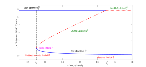
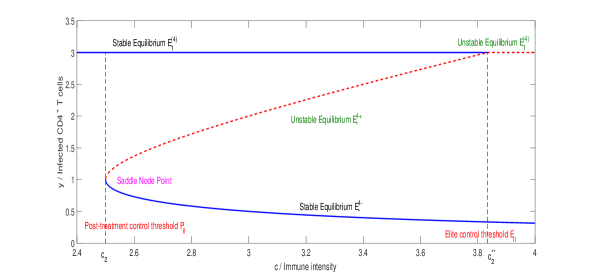
Remark 3.1 If $\mathcal{R}^{(2)}_{0}>\mathcal{R}^{(1)}_{c}>1$ and $c_{2}<c<c^{**}_{1}$, system (1.3) has bistability appear. In other cases, system (1.3) has no bistability appear. Threshold $c_{2}$ is a post-treatment control threshold, $c^{**}_{1}$ is a elite control threshold. $(c_{2},c^{**}_{1})$ is a bistable interval.

To sum up, the stabilities of the equilibria and the behaviors of system (1.3) can be shown in Table 3 and Table 4.

3.5 Numerical simulations and discussion

To verify our analysis results, we carry out some numerical simulations choosing some parameter values shown as in [21, 24, [24]]:

$$\begin{array}[]{lll}&&s=10~{}~{}cells/\mu l/day,\hskip 0.56917ptd=0.01~{}~{}\mbox{day}^{-1},\hskip 0.56917pt\epsilon=0.9,\\ &&\beta=0.015~{}~{}\mu l/day,\hskip 0.56917pta=1.1~{}~{}\mbox{day}^{-1},\hskip 0.56917ptp=0.5~{}~{}\mbox{day}^{-1},\\ &&\alpha=1~{}~{}cells/\mu l,\hskip 0.56917pt\gamma=1~{}~{}cells/\mu l,\hskip 0.56917ptb=0.1~{}~{}\mbox{day}^{-1}.\end{array}$$

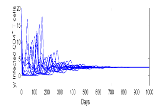
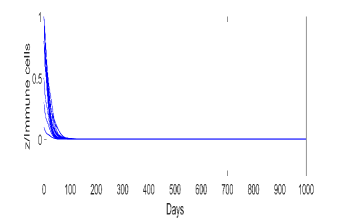
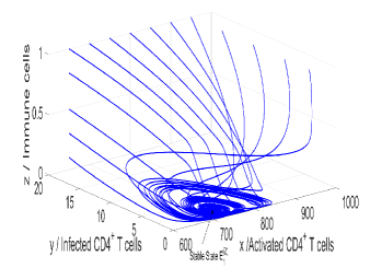
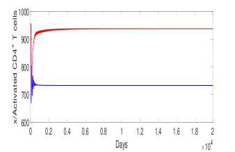
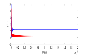
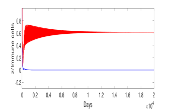
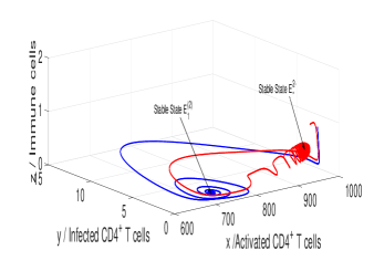
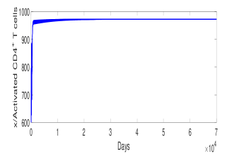
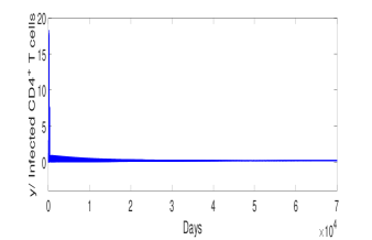
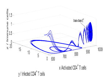
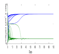
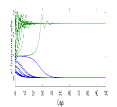
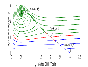
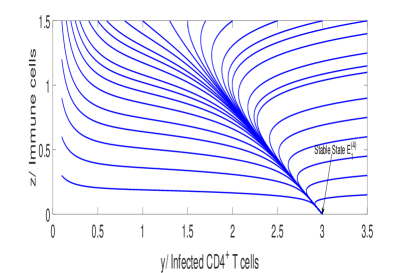
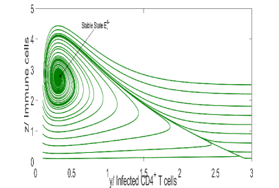
The parameters chose as same as in (3.1), the thresholds $\mathcal{R}^{(2)}_{0}\approx 1.3636$, $\mathcal{R}^{(1)}_{c}=1.1500,$ post-treatment control threshold $c_{2}=0.3000$ and elite control threshold $c^{**}_{1}\approx 0.3837$. In this case, $\mathcal{R}^{(2)}_{0}>\mathcal{R}^{(1)}_{c}$ and $c_{2}<c^{**}_{1}$, then we get a bistable interval $(0.3000,0.3837)$ (see Figure 1). When $0<c<c_{2}$, the immune-free equilibrium $E^{(2)}_{1}$ is stable (see Fig. 2); When $c_{2}<c<c^{**}_{1}$, the immune-free equilibrium $E^{(2)}_{1}$ and the positive equilibrium $E_{*}^{2-}$ are stable (see Fig. 3); When $c>c^{**}_{1}$, only the positive equilibrium $E_{*}^{2-}$ is stable (see Figure 4).

Figure 1: Bistability and saddle-node bifurcation diagram of system (1.3). The solid line is the stable infected CD4+ T cells and the dashed line depends the unstable infected CD4+ T cells. The post-treatment control threshold is $c_{2}=0.2500$, the elite control threshold is $c^{**}_{1}\approx 0.6505$ and the bistable interval is $(0.2500,0.6505).$ $c=0.37~{}~{}\mbox{day}^{-1}$ and other parameter values are shown in (3.1).

Figure 2: System (1.3) has a stable equilibria $E^{(2)}_{1}$. Parameter $c=0.2~{}~{}\mbox{day}^{-1}$ less than post-treatment control threshold $P_{I}$ and other parameter values are shown in (3.1). We choose different initial values.

Figure 3: System (1.3) has two different stable equilibria $E^{(2)}_{1}$ and $E_{-}^{2*}$. Parameter $c=0.37~{}~{}\mbox{day}^{-1}$ and other parameter values are shown in (3.1). We choose different initial values.

Figure 4: System (1.3) has only the positive equilibrium $E_{-}^{2*}$ is stable. Parameter $c=0.65~{}~{}\mbox{day}^{-1}$ and other parameter values are shown in (3.1). We choose different initial values.

4 2D-Viral infection system with monotonic immune response

In this section, we discuss 2D viral infection system with monotonic immune response.

$$\left\{\begin{array}[]{l l}\frac{dy}{dt}=\gamma y(1-\frac{y}{K})-ay-pyz=P_{1},\\ \frac{dz}{dt}=f(y)z-bz=Q_{1},\end{array}\right.$$

where $f(y)$ is a monotonic function of $y$ and satisfies (1.2).

System (4.1) always has an uninfected steady equilibrium $E^{(3)}_{0}=(0,0)$, and if ${R}^{(2)}_{0}>1$, system (4.1) also has an immune-free equilibrium $E^{(3)}_{1}=(y^{(3)}_{1},0)$; If $\mathcal{R}_{*}^{(2)}>1$ system (4.1) has three equilibria $E^{(3)}_{0}$, $E^{(3)}_{1}$ and $E_{*}^{(3)}=(y_{*}^{(3)},z_{*}^{(3)})$, where

$$\begin{array}[]{ll}\displaystyle y^{(3)}_{1}=\frac{aK}{\gamma}({R}^{(3)}_{0}-1),\\ \vspace{2\jot}y^{(3)}_{*}=f^{-1}(b),\\ \vspace{2\jot}\displaystyle z^{(3)}_{*}=\frac{a}{p}(\mathcal{R}_{*}^{(2)}-1).\end{array}$$

We give a threshold

$$\mathcal{R}^{(3)}_{0}=\frac{\gamma}{a},$$

and the basic immune reproductive number is

$$\mathcal{R}_{*}^{(2)}=\frac{\gamma}{a}(1-\frac{y^{(3)}_{*}}{K}).$$

This ratio describes the average number of newly infected cells generated form on infected cell at the beginning of the infectious process.

Let $\tilde{E}$ be any arbitrary equilibrium of system (4.1). The Jacobian matrix associated with the system is

$$J_{3}=\left[\begin{array}[]{cccc}\gamma-a-\frac{2\gamma}{k}\tilde{y}-p\tilde{z}&-p\tilde{y}\\ f^{{}^{\prime}}(\tilde{y})\tilde{z}&f(\tilde{y})-b\\ \end{array}\right].$$

The characteristic equation of the linearized system of (4.1) at $\tilde{E}$ is given by $\left|\lambda I-J_{3}\right|=0.$

Lemma 4.1 $\mathcal{R}_{*}^{(2)}<1\Leftrightarrow y^{(3)}_{1}<y_{*}^{(3)}$.

Proof.

$$\begin{array}[]{lll}R_{*}^{(2)}<1&\Leftrightarrow&\frac{\gamma}{a}(1-\frac{y_{*}^{(3)}}{K})<1,\\ &\Leftrightarrow&\frac{Ka}{\gamma}({R}^{(3)}_{0}-1)<y_{*}^{(3)},\\ &\Leftrightarrow&y^{(3)}_{1}<y_{*}^{(3)}.\end{array}$$

Lemma 4.2 System (4.1) has no limit cycles in the interior of the first quadrant.

Proof. Consider the Dulac function

$$D_{1}=\frac{1}{yz}.$$

We can get

$$\begin{array}[]{lll}\begin{split}&\displaystyle\frac{\partial(D_{1}P_{1})}{\partial y}+\frac{\partial(D_{1}Q_{1})}{\partial z}\\ &=\frac{\partial[\frac{1}{yz}(\gamma y(1-\frac{y}{K})-ay-pyz)]}{\partial y}+\frac{\partial[\frac{1}{yz}(f(y)z-bz)]}{\partial z}\vspace{0.2cm}\\ &=\displaystyle\frac{\partial(\frac{\gamma}{z}-\frac{\gamma y}{Kz}-\frac{a}{z}-p)}{\partial y}+\frac{\partial(\frac{f(y)}{y}-\frac{b}{y})}{\partial z}\vspace{0.2cm}\\ &=-\frac{\gamma}{Kz}\leq 0.\end{split}\end{array}$$

By $Bendixson-Dulac$ discriminant method, we know system (4.1) has no limit cycles.

Theorem 4.1   If $\mathcal{R}^{(3)}_{0}<1$, then the uninfected equilibrium $E^{(3)}_{0}$ of system (4.1) is not only locally asymptotically stable, but also global asymptotically stable. If $\mathcal{R}^{(3)}_{0}>1$. then the uninfected equilibrium $E^{(3)}_{0}$ of system (4.1) is unstable.

Proof. The characteristic equation of the linearized system of system (4.1) at $E^{(3)}_{0}$ is

$$(\lambda+a-\gamma)(\lambda+b)=0.$$

Obviously, the characteristic roots $-b$ and $a(\mathcal{R}^{(3)}_{0}-1)$ are negative for $\mathcal{R}^{(3)}_{0}<1$. Hence $E^{(3)}_{0}$ is locally asymptotically stable. If $\mathcal{R}^{(3)}_{0}>1$, then $a(\mathcal{R}^{(3)}_{0}-1)>0$, thus, the uninfected equilibrium $E^{(3)}_{0}$ of system (4.1) is unstable. By Lemma 4.2, the uninfected equilibrium $E^{(3)}_{0}$ is global asymptotically stable. Theorem 4.1 is proved.

Theorem 4.2   If $\mathcal{R}^{(3)}_{0}>1>\mathcal{R}^{(2)}_{*}$, then the immune-free equilibrium $E^{(3)}_{1}$ of system (4.1) is not only locally asymptotically stable, but also global asymptotically stable. $E^{(3)}_{1}$ is unstable for $\mathcal{R}^{(2)}_{*}>1$.

Proof. The characteristic equation of the linearized system of (4.1) at $E^{(3)}_{1}$ is given by

$$(\lambda+\frac{\gamma}{k}y^{(3)}_{1})[\lambda-(f(y^{(3)}_{1})-b)]=0.$$

By Lemma 4.1 and $f^{{}^{\prime}}(y)>0$ for $[0,+\infty)$ and $f(y^{(3)}_{*})=b$, we deduce the eigenvalue $\lambda=f(y^{(3)}_{1})-b<0$ for $\mathcal{R}^{(3)}_{0}>1>\mathcal{R}^{(2)}_{*}$, and $\lambda=f(y^{(3)}_{1})-b>0$ for ${R}^{(2)}_{*}>1$. Thus, the immune-free equilibrium $E^{(3)}_{1}$ of system (4.1) is locally asymptotically stable for $\mathcal{R}^{(3)}_{0}>1>\mathcal{R}^{(2)}_{*}$ and is unstable for $\mathcal{R}^{(2)}_{*}>1$. By Lemma 4.2, the immune-free equilibrium $E^{(3)}_{1}$ is global asymptotically stable. Theorem 4.2 is proved.

Theorem 4.3   If $\mathcal{R}^{(2)}_{*}>1$, then the positive equilibrium $E^{(3)}_{*}$ of system (4.1) is not only locally asymptotically stable, but also global asymptotically stable.

Proof. The characteristic equation of the linearized system of (4.1) at $E^{(3)}_{*}$ is given by

$$\lambda^{2}+a^{(3)}_{1}\lambda+a^{(3)}_{2}=0,$$

where

$$\begin{array}[]{lll}a^{(3)}_{1}&=&\frac{\gamma}{k}y^{(3)}_{*}+b-f(y^{(3)}_{*}),\\ a^{(3)}_{2}&=&\frac{\gamma}{k}y^{(3)}_{*}[b-f(y^{(3)}_{*})]+py^{(3)}_{*}z^{(3)}_{*}f^{{}^{\prime}}(y^{(3)}_{*}).\end{array}$$

By Lemma 4.1 and $f^{{}^{\prime}}(y)>0$ for $[0,+\infty)$ and $f(y^{(3)}_{*})=b$, we know $a^{(3)}_{1}>0$ and $a^{(3)}_{2}>0$. By Routh-Hurartz Criterion, we know the positive equilibrium $E^{(3)}_{*}$ of system (4.1) is locally asymptotically stable for $\mathcal{R}^{(2)}_{*}>1$. By Lemma 4.2, the positive equilibrium $E^{(3)}_{*}$ is global asymptotically stable. Theorem 4.3 is proved.

By Theorem 4.1$\sim$4.3, we can get following result:

Remark 4.1 Viral infection system with monotonic immune response has no bistability appear.

5 2D-Viral infection system with nonmonotonic immune response

In this section, we will discuss the 2D-viral infection system with Monod-Haldane function, which is a system with nonmonotonic immune response.

$$\left\{\begin{array}[]{l l}\frac{dy}{dt}=\gamma y(1-\frac{y}{K})-ay-pyz=P_{2},\\ \frac{dz}{dt}=\frac{cyz}{\alpha+\gamma y+y^{2}}-bz=Q_{2},\end{array}\right.$$

We always assume $K>\sqrt{\alpha}$. The threshold ${R}^{(4)}_{0}=\frac{\gamma}{a}$, which is equivalent to ${R}^{(3)}_{0}$.

(i) System (5.1) always has an uninfected steady equilibrium $E^{(4)}_{0}=(0,0)$, and if $R^{(4)}_{0}>1$, system (5.1) also has an immune-free equilibrium $E^{(4)}_{1}=(y^{(4)}_{1},0)$, where $y^{(4)}_{1}=\frac{Ka}{\gamma}({R}^{(4)}_{0}-1)$.

Solving equation $\frac{cy}{\alpha+\gamma y+y^{2}}-b=0$, one get two positive roots, $c_{1}=\gamma b-2b\sqrt{\alpha}$ and $c_{2}=\gamma b+2b\sqrt{\alpha}$ , then the existence conditions of positive equilibria as following:

(ii) If $\mathcal{R}_{*}^{2-}>1$ and $c>c_{2},$ system (5.1) has an immune equilibrium $E_{*}^{4-}=(y_{*}^{4-},z_{*}^{4-})$; If $\mathcal{R}_{*}^{2+}>1$ and $c>c_{2},$ system (1.3) also has an immune equilibrium $E_{*}^{4+}=(y_{*}^{4+},z_{*}^{4+}).$ Here $\mathcal{R}^{2\pm}_{*}=\frac{\gamma}{a}(1-\frac{y^{4\pm}_{*}}{K}),y^{4\pm}_{*}=\frac{-B\pm\sqrt{B^{2}-4\alpha b^{2}}}{2b},z^{4\pm}_{*}=\frac{a}{p}({R}^{2\pm}_{*}-1),B=\gamma b-c.$

We denote post-treatment control threshold $P_{II}$ (see e.g. Refs [21])

$$c_{2}=\gamma b+2b\sqrt{\alpha}.$$

Which is equivalent to post-treatment control threshold $P_{I}$ .

Denote

$$c^{*}_{2}=\gamma b+\frac{2baK(\mathcal{R}^{(4)}_{0}-1)}{\gamma},$$

$$c^{**}_{2}=\gamma b+\frac{baK(\mathcal{R}^{(4)}_{0}-1)}{\gamma}+\frac{b\alpha\gamma}{aK({R}^{(4)}_{0}-1)},$$

We call $c^{**}_{2}$ the elite control threshold $E_{II}$, [21] which means the virus will be under control when the immune intensity $c$ is larger than $c^{**}_{2}$.

Denote another threshold

$$\mathcal{R}^{(2)}_{c}=1+\frac{\sqrt{\alpha}}{K-\sqrt{\alpha}}.$$

For the positive parameters in model (5.1), we have the following lemmas.

Lemma 5.1 $\mathcal{R}^{(4)}_{0}>\mathcal{R}^{(2)}_{c}>1\Leftrightarrow c^{*}_{2}>c^{**}_{2}.$

Proof.

$$\begin{array}[]{lll}c^{*}_{2}>c^{**}_{2}&\Leftrightarrow&\frac{baK({R}^{(4)}_{0}-1)}{\gamma}>\frac{b\alpha\gamma}{aK(\mathcal{R}^{(4)}_{0}-1)},\\ &\Leftrightarrow&\mathcal{R}^{(4)}_{0}>\mathcal{R}^{(2)}_{c}.\end{array}$$

Lemma 5.2 (i) $\mathcal{R}^{(4)}_{0}>\mathcal{R}^{(2)}_{c}>1\Leftrightarrow c^{*}_{2}>c_{2}$; (ii) $1<\mathcal{R}^{(4)}_{0}<\mathcal{R}^{(2)}_{c}\Leftrightarrow c^{*}_{2}<c_{2}.$

Proof.

$$\begin{array}[]{lll}c^{*}_{2}>c_{2}&\Leftrightarrow&\frac{baK(\mathcal{R}^{(4)}_{0}-1)}{\gamma}>b\sqrt{\alpha},\\ &\Leftrightarrow&\mathcal{R}^{(4)}_{0}>R^{(2)}_{c}.\end{array}$$

$$\begin{array}[]{lll}c^{*}_{2}<c_{2}&\Leftrightarrow&\frac{baK(\mathcal{R}^{(4)}_{0}-1)}{\gamma}<b\sqrt{\alpha},\\ &\Leftrightarrow&\mathcal{R}^{(4)}_{0}<R^{(2)}_{c}.\end{array}$$

Lemma 5.3 (i) Assume $1<\mathcal{R}^{(4)}_{0}<\mathcal{R}^{(2)}_{c}.$ If $\mathcal{R}_{*}^{2-}>1$, then $c>c^{**}_{2}$; (ii) Assume $\mathcal{R}^{(4)}_{0}>\mathcal{R}^{(2)}_{c}>1.$ If $\mathcal{R}_{*}^{2-}>1$, then $c>c_{2}$.

Proof.

$$\begin{array}[]{lll}\mathcal{R}_{*}^{2-}>1&\Leftrightarrow&\frac{\gamma}{a}(1-\frac{y_{*}^{4-}}{K})>1,\\ &\Leftrightarrow&\sqrt{(\gamma b-c)^{2}-4\alpha b^{2}}>c-c^{*}_{2}.\end{array}$$

If $c<c^{*}_{2}$ and one of conditions $c<c_{1}$ or $c>c_{2}$ is correct, then $\mathcal{R}_{*}^{2-}$ is always larger than one. If $c>c^{*}_{2}$, solving $\sqrt{(\gamma b-c)^{2}-4\alpha b^{2}}>c-c^{*}_{2}$, we have $c>c^{**}_{2}.$ Thus,

(i) If $1<\mathcal{R}^{(4)}_{0}<\mathcal{R}^{(2)}_{c}$, then $c^{*}_{2}<c_{2}$. From $\mathcal{R}_{*}^{2-}>1$, we have $c>c^{**}_{2}.$

(ii) If $\mathcal{R}^{(4)}_{0}>\mathcal{R}^{(2)}_{c}>1$, then $c^{*}_{2}>c_{2}$. From $\mathcal{R}_{*}^{2-}>1$, we have $c>c_{2}.$

Lemma 5.4 (i) If $1<\mathcal{R}^{(4)}_{0}<\mathcal{R}^{(2)}_{c},$ then $\mathcal{R}_{*}^{2+}>1$ has no solution; (ii) Assume $\mathcal{R}^{(4)}_{0}>\mathcal{R}^{(2)}_{c}>1$. If $\mathcal{R}_{*}^{2+}>1$, then $c_{2}<c<c^{**}_{2}$.

Proof.

$$\begin{array}[]{lll}\mathcal{R}_{*}^{2+}>1&\Leftrightarrow&\frac{\gamma}{a}(1-\frac{y_{*}^{4+}}{K})>1,\\ &\Leftrightarrow&c^{*}-c>\sqrt{(\gamma b-c)^{2}-4\alpha b^{2}}.\end{array}$$

(i) If $1<{R}^{(4)}_{0}<R^{(2)}_{c},$ then $c^{*}_{2}<c_{2}$. Thus $\mathcal{R}_{*}^{2+}>1$ has no solution. (ii) If $\mathcal{R}^{(4)}_{0}>\mathcal{R}^{(2)}_{c}>1$, then $c^{*}_{2}>c_{2}$. Solving $\mathcal{R}_{*}^{2+}>1$, we have $c_{2}<c<c^{**}_{2}$.

By Lemma 5.1 $\sim$ Lemma 5.4 and summing up the above analysis we obtain the existing results of equilibria of system (5.1).

Theorem 5.1 (i) System (5.1) always exists an uninfected equilibrium $E^{(4)}_{0}=(0,0);$

(ii) If $\mathcal{R}^{(4)}_{0}>1$, system (5.1) also has an immune-free equilibrium $E^{(4)}_{1}=(y^{(4)}_{1},0),$ where $y^{(4)}_{1}=\frac{aK}{\gamma}(R^{(4)}_{0}-1)$;

(iii) If $1<\mathcal{R}^{(4)}_{0}<\mathcal{R}^{(2)}_{c}$ and $c>c^{**}_{2},$ system (5.1) also has one positive equilibrium $E_{*}^{4-};$

(iv) If $\mathcal{R}^{(4)}_{0}>\mathcal{R}^{(2)}_{c}>1$ and $c_{2}<c<c^{**}_{2}$, system (5.1) has two positive equilibria $E_{*}^{4+}$ and $E_{*}^{4-}$. While $\mathcal{R}^{(4)}_{0}>\mathcal{R}^{(2)}_{c}$ and $c>c^{**}_{2}$, system (5.1) only has one positive equilibrium $E_{*}^{4-}$;

The summary results of the existence for positive equilibria can be seen in Table 5 and Table 6.

5.1 Stability analysis

Let $\tilde{E}$ be any arbitrary equilibrium of system (5.1). The Jacobian matrix associated with the system is

$$J_{4}=\left[\begin{array}[]{cccc}\gamma-a-\frac{2\gamma}{K}y-pz&-py\\ \frac{(\alpha-y^{2})cz}{(\alpha+\gamma y+y^{2})^{2}}&\frac{cy}{\alpha+\gamma y+y^{2}}-b\\ \end{array}\right].$$

The characteristic equation of the linearized system of (5.1) at $\tilde{E}$ is given by $\left|\lambda I-J_{4}\right|=0.$

Lemma 5.5 System (5.1) has no limit cycles in the interior of the first quadrant.

Proof. Consider the Dulac function

$$D_{2}=\frac{1}{yz}.$$

We can get

$$\begin{array}[]{lll}\begin{split}&\displaystyle\frac{\partial(D_{2}P_{2})}{\partial y}+\frac{\partial(D_{2}Q_{2})}{\partial z}\\ &=\frac{\partial[\frac{1}{yz}(\gamma y(1-\frac{y}{K})-ay-pyz)]}{\partial y}+\frac{\partial[\frac{1}{yz}(\frac{cyz}{\alpha+\gamma y+y^{2}}-bz)]}{\partial z}\\ &=\displaystyle\frac{\partial(\frac{\gamma}{z}-\frac{\gamma y}{Kz}-\frac{a}{z}-p)}{\partial y}+\frac{\partial(\frac{c}{\alpha+\gamma y+y^{2}}-\frac{b}{y})}{\partial z}\vspace{0.2cm}\\ &=-\frac{\gamma}{Kz}\leq 0.\end{split}\end{array}$$

By Bendixson-Dulac discriminant method, we know system (5.1) has no limit cycles. 

Theorem 5.2   If $\mathcal{R}^{(4)}_{0}<1$, then the uninfected equilibrium $E^{(4)}_{0}$ of system (5.1) is not only locally asymptotically stable, but also global asymptotically stable. If $\mathcal{R}^{(4)}_{0}>1$. then the uninfected equilibrium $E^{(4)}_{0}$ of system (5.1) is unstable.

Proof. The characteristic equation of the linearized system of system (5.1) at $E^{(4)}_{0}$ is

$$(\lambda+a-\gamma)(\lambda+b)=0.$$

Obviously, the characteristic roots $-b$ and $a(\mathcal{R}^{(4)}_{0}-1)$ are negative for $\mathcal{R}^{(4)}_{0}<1$. Hence $E^{(4)}_{0}$ is locally asymptotically stable. If $\mathcal{R}^{(4)}_{0}>1$, then $a(\mathcal{R}^{(4)}_{0}-1)>0$, thus, the uninfected equilibrium $E^{(4)}_{0}$ of system (5.1) is unstable. By Lemma 5.5, the uninfected equilibrium $E^{(4)}_{0}$ is global asymptotically stable. Theorem 5.2 is proved.

Theorem 5.3   If $\mathcal{R}^{(4)}_{0}>1$ and $0<c<c^{**}_{2}$, then the immune-free equilibrium $E^{(4)}_{1}$ of system (5.1) is not only locally asymptotically stable, but also global asymptotically stable.

Proof. The characteristic equation of the linearized system of (5.1) at $E^{(4)}_{1}$ is given by

$$[\lambda-(\gamma-a-\frac{2\gamma}{K}y^{(4)}_{1})][\lambda-(\frac{cy^{(4)}_{1}}{\alpha+\gamma y^{(4)}_{1}+{(y^{(4)}_{1}})^{2}}-b)]=0,$$

we get two eigenvalues $\lambda_{1}=\gamma-a-\frac{2\gamma}{K}y^{(4)}_{1}=a(1-\frac{\gamma}{a})<0$ for $\mathcal{R}^{(4)}_{0}>1$, and $\lambda_{2}=\frac{cy^{(4)}_{1}}{\alpha+\gamma y^{(4)}_{1}+{(y^{(4)}_{1}})^{2}}-b>0$ for $0<c<c^{**}_{2}$. Thus, the immune-free equilibrium $E^{(4)}_{1}$ of system (5.1) is locally asymptotically stable for $\mathcal{R}^{(4)}_{0}>1$ and $0<c<c^{**}_{2}$. By Lemma 5.5, the immune-free equilibrium $E^{(4)}_{1}$ is global asymptotically stable. Theorem 5.3 is proved.

Theorem 5.4 (i) If   ($\mathbf{A.1}$)    $1<\mathcal{R}^{(4)}_{0}<\mathcal{R}^{(2)}_{c}$ and $c>c^{**}_{2}$, or

($\mathbf{A.2}$)    $\mathcal{R}^{(4)}_{0}>\mathcal{R}^{(2)}_{c}$ and $c>c_{2}$,
system (5.1) has an immune equilibrium $E_{*}^{4-},$ which is not only asymptotically stable, but also global asymptotically stable.

(ii) If $\mathcal{R}^{(4)}_{0}>\mathcal{R}^{(2)}_{c}$ and $c_{2}<c<c^{**}_{2}$, system (5.1) also has an immune equilibrium $E_{*}^{4+},$ which is an unstable saddle.

Proof. Denote $E_{*}^{(4)}=(y_{*}^{(4)},z_{*}^{(4)})$ as an arbitrary positive equilibrium of system (5.1). The characteristic equation of the linearized system of (5.1) at the arbitrary positive equilibrium $E_{*}^{(4)}$ is given by

$$\lambda^{2}+b^{(4)}_{1}\lambda+b^{(4)}_{2}=0,$$

where

$$\begin{array}[]{lll}b^{(4)}_{1}&=&\frac{\gamma}{K}y_{*}^{(4)}>0,\\ b^{(4)}_{2}&=&\frac{\alpha-(y_{*}^{(4)})^{2}}{(\alpha+\gamma y_{*}^{(4)}+(y_{*}^{(4)})^{2})^{2}}pcy_{*}^{(4)}z_{*}^{(4)}.\end{array}$$

For equilibrium $E_{*}^{4-},$

$$\begin{array}[]{lll}\alpha-(y_{*}^{4-})^{2}>0&\Leftrightarrow&\frac{-B-\sqrt{B^{2}-4\alpha b^{2}}}{2b}<\sqrt{\alpha},\\ &\Leftrightarrow&c>c_{2}.\end{array}$$

If $c>c_{2}$, we can get $b^{(4)}_{2}>0$, by Routh-Hurartz Criterion, we know in this case the positive equilibrium $E_{*}^{4-}$ is a stable node.

For equilibrium $E_{*}^{4+},$

$$\begin{array}[]{lll}\alpha-(y_{*}^{4+})^{2}<0&\Leftrightarrow&\frac{-B+\sqrt{B^{2}-4\alpha b^{2}}}{2b}>\sqrt{\alpha},\\ &\Leftrightarrow&\sqrt{B^{2}-4\alpha B^{2}}>B+2b\sqrt{\alpha}.\end{array}$$

If $c_{2}<c<c^{**}_{2}$, then $b^{(4)}_{2}<0$, so the immune equilibrium $E_{*}^{4+}$ is an unstable saddle. By Lemma 5.5, the immune equilibrium $E_{*}^{4-},$ is global asymptotically stable. Theorem 5.4 is proved.

5.2 Saddle-node Bifurcation

If $\mathcal{R}^{(4)}_{0}>\mathcal{R}^{(2)}_{c}>1$ and $c^{2}-2\gamma bc+\gamma^{2}b^{2}-4\alpha b^{2}=0$, the immune equilibrium $E_{*}^{4+}$ and $E_{*}^{4-}$ coincide with each other. Then system has the unique interior equilibrium $E_{*}=(y_{*},z_{*})=(\sqrt{\alpha},\frac{a}{pR_{c}}(R_{0}-R_{c}))$. The emergence and disappearance of the equilibrium is due to the occurrence of saddle-node bifurcation when $c$ crosses the bifurcation value $c^{[sn]}$, where $c^{[sn]}=\gamma b+2b\sqrt{\alpha}$.

Theorem 5.5 If $\mathcal{R}^{(4)}_{0}>\mathcal{R}^{(2)}_{c}>1$ and $c=c^{[sn]}$, system (5.1) will undergoes a saddle-node bifurcation, $c$ as the bifurcation parameter is given by $c=c^{[sn]}=\gamma b+2b\sqrt{\alpha}$.

Proof. We use Sotomayor’s theorem [26, 27, 28] to prove system (5.1) undergoes a saddle-node bifurcation at $c=c^{[sn]}$. It’s easy to prove $Det[J_{E_{*}}]=0$, so one of the eigenvalue of the Jacobian at the saddle-node equilibrium is zero, where $J=J_{4}$.

Let $V=(V_{1},V_{2})^{\mathrm{T}}$ and $W=(W_{1},W_{2})^{\mathrm{T}}$ represent the eigenvectors of $J_{E_{*}}$ and $J_{E_{*}}^{\mathrm{T}}$ corresponding to the zero eigenvalue, respectively, then they are given by $V=(1,-\frac{\gamma}{Kp})^{\mathrm{T}}$ and $W=(0,1)^{\mathrm{T}}$. Let $F=(P_{2},Q_{2})$, we can get

$$F_{c}(E_{*};c^{[sn]})=\left[\begin{array}[]{cccc}0\\ \frac{yz}{\alpha+\gamma y+y^{2}}\end{array}\right]_{(E_{*};c^{[sn]})}=\left[\begin{array}[]{cccc}0\\ \frac{\gamma(1-\frac{\sqrt{\alpha}}{K})-a}{p(2\sqrt{\alpha}+\gamma)}\end{array}\right],$$

and

$$\begin{array}[]{lll}\begin{split}\displaystyle&D^{2}F(E_{*};c^{[sn]})(V,V)\\ &=\left[\begin{array}[]{cccc}0\\ \frac{-6c\alpha yz+2czy^{3}-2c\alpha\gamma z}{(\alpha+\gamma y+y^{2})^{3}}-\frac{2\gamma c(\alpha-y^{2})}{pK(\alpha+\gamma y+y^{2})^{2}}\end{array}\right]_{(E_{*};c^{[sn]})}\\ &=\left[\begin{array}[]{cccc}0\\ \frac{-2\alpha z_{*}(\gamma b+2b\sqrt{\alpha})(2\sqrt{\alpha}+\gamma)}{(\alpha+\gamma y_{*}+y_{*}^{2})^{3}}\end{array}\right].\end{split}\end{array}$$

Therefore,

$$\begin{array}[]{lll}\begin{split}\Omega_{1}&=W^{\mathrm{T}}F_{c}(E_{*},c^{[sn]})=\frac{\gamma(1-\frac{\sqrt{\alpha}}{K})-a}{p(2\sqrt{\alpha}+\gamma)}\neq 0,\vspace{0.2cm}\\ \Omega_{2}&=W^{\mathrm{T}}[D^{2}F(E_{*};c^{[sn]})(V,V)]=\frac{-2\alpha z_{*}(\gamma b+2b\sqrt{\alpha})(2\sqrt{\alpha}+\gamma)}{(\alpha+\gamma y_{*}+y_{*}^{2})^{2}}\neq 0.\end{split}\end{array}$$

Therefore, from the Sotomayor’ s theorem, [26, 27, 28] system (5.1) undergoes a saddle-node bifurcation at $E_{*}=(y_{*},z_{*})$ when $c=c^{[sn]}$. Hence, we can conclude that when parameter $c$ passes from one side from of $c=c^{[sn]}$ to the other side, the number of interior equilibrium of system (5.1) changes from zero to two.

5.3 Transcritical Bifurcation

From the stability analysis of system (5.1), the boundary equilibrium $E_{1}^{(4)}$ looses its stability at $c=\gamma b+\frac{baK(\mathcal{R}^{(4)}_{0}-1)}{\gamma}+\frac{b\alpha\gamma}{aK(\mathcal{R}^{(4)}_{0}-1)}$ and one of the eigenvalue of the Jacobian at $E_{1}^{(4)}$ is zero. Therefore, bifurcation may occur at the boundary equilibrium $E_{1}^{(4)}$. In this section, we select parameter $c$ as bifurcation parameter to study the existence of a transcritical bifurcation.

Theorem 5.6 If $R_{0}>1$ and $c=c^{[tc]}$, system (5.1) will undergoes a transcritical bifurcation between $E_{1}^{(4)}$ and $E_{*}^{4-}$, $c$ as the bifurcation parameter is given by $c=c^{[tc]}=\gamma b+\frac{baK({R}^{(4)}_{0}-1)}{\gamma}+\frac{b\alpha\gamma}{aK({R}^{(4)}_{0}-1)}$.

Proof. We use Sotomayor’s theorem [26, 27, 28] to prove system (5.1) undergoes a transcritical bifurcation. Obviously, one of the eigenvalue of the Jacobian at $E_{1}^{(4)}$ is zero, if and only if $c=c^{[tc]}$.

Let $\nu=(\nu_{1},\nu_{2})^{\mathrm{T}}$ and $\omega=(\omega_{1},\omega_{2})^{\mathrm{T}}$ denote the eigenvectors of $J_{E_{1}^{(4)}}$ and $J_{E_{1}^{(4)}}^{\mathrm{T}}$ corresponding to the zero eigenvalue, respectively, we can get $\nu=(1,-\frac{\gamma}{Kp})^{\mathrm{T}}$ and $\omega=(0,1)^{\mathrm{T}}$, Besides,

$$F_{c}(E_{1}^{(4)};c^{[tc]})=\left[\begin{array}[]{cccc}0\\ \frac{yz}{\alpha+\gamma y+y^{2}}\end{array}\right]_{(E_{1}^{(4)};c^{[tc]})}=\left[\begin{array}[]{cccc}0\\ 0\end{array}\right].$$

$$\begin{array}[]{lll}\begin{split}\displaystyle&DF_{c}(E_{1}^{(4)};c^{[tc]})\nu\\ &=\left[\begin{array}[]{cccc}0\\ \frac{\alpha z-zy^{2}}{(\alpha+\gamma y+y^{2})^{2}}-\frac{\gamma y}{Kp(\alpha+\gamma y+y^{2})}\end{array}\right]_{(E_{1}^{(4)};c^{[tc]})}\\ &=\left[\begin{array}[]{cccc}0\\ -\frac{\gamma y_{1}^{(4)}}{Kp(\alpha+\gamma y_{1}^{(4)}+{y_{1}^{(4)}}^{2})}\end{array}\right].\end{split}\end{array}$$

$$\begin{array}[]{lll}\begin{split}\displaystyle&D^{2}F(E_{1}^{(4)};c^{[tc]})(\nu,\nu)\\ &=\left[\begin{array}[]{cccc}0\\ \frac{-6c\alpha yz+2czy^{3}-2c\alpha\gamma z}{(\alpha+\gamma y+y^{2})^{3}}-\frac{2\gamma c(\alpha-y^{2})}{pK(\alpha+\gamma y+y^{2})^{2}}\end{array}\right]_{(E_{1}^{(4)};c^{[tc]})}\\ &=\left[\begin{array}[]{cccc}0\\ \frac{-2\gamma(\gamma b+\frac{baK({R}^{(4)}_{0}-1)}{r}+\frac{b\alpha r}{aK({R}^{(4)}_{0}-1)})(\alpha-{y_{1}^{(4)}}^{2})}{(\alpha+\gamma y_{1}^{(4)}+{y_{1}^{(4)}}^{2})^{2}}\end{array}\right].\end{split}\end{array}$$

Therefore,

$$\begin{array}[]{lll}\begin{split}\Phi_{1}&=\omega^{\mathrm{T}}F_{c}(E_{1}^{(4)};c^{[tc]})=0,\vspace{0.2cm}\\ \Phi_{2}&=\omega^{\mathrm{T}}[DF_{c}(E_{1}^{(4)};c^{[tc]})\eta]=-\frac{\gamma y_{1}^{(4)}}{Kp(\alpha+\gamma y_{1}^{(4)}+{y_{1}^{(4)}}^{2})}\neq 0\\ \Phi_{3}&=\omega^{\mathrm{T}}[D^{2}F(E_{1}^{(4)};c^{[tc]})(\nu,\nu)]=\frac{-2\gamma(\gamma b+\frac{baK({R}^{(4)}_{0}-1)}{\gamma}+\frac{b\alpha\gamma}{aK({R}^{(4)}_{0}-1)})(\alpha-{y_{1}^{(4)}}^{2})}{(\alpha+\gamma y_{1}^{(4)}+{y_{1}^{(4)}}^{2})^{2}}\neq 0.\end{split}\end{array}$$

Therefore, system (5.1) will undergoes a transcritical bifurcation between $E_{1}^{(4)}$ and $E_{*}^{4-}$ at $c=c^{[tc]}$

Remark 5.1 If $\mathcal{R}^{(4)}_{0}>\mathcal{R}^{(4)}_{c}>1$ and $c_{2}<c<c^{**}_{2}$, system (5.1) has bistability appear. In other cases, system (5.1) has no bistability appear. Threshold $c_{2}$ is the post-treatment control threshold, $c^{**}_{2}$ is the elite control threshold. $(c_{2},c^{**}_{2})$ is the bistable interval.

To sum up, the stabilities of the equilibria and the behaviors of system (5.1) can be shown in Table 7 and Table 8.

5.4 Numerical simulations and discussion

To verify our analysis results, we carry out some numerical simulations choosing some parameter values shown as in [[24], 25]:

$$\begin{array}[]{lll}&&\gamma=6~{}~{}\mbox{day}^{-1},\hskip 0.56917ptK=6~{}~{}cells/\mu l,\hskip 0.56917pta=3~{}~{}\mbox{day}^{-1},\\ &&p=1~{}~{}\mbox{day}^{-1},\hskip 0.56917pt\alpha=1~{}~{}cells/\mu l,\hskip 0.56917pt\gamma=0.5~{}~{}cells/\mu l,\\ &&b=1~{}~{}\mbox{day}^{-1}.\end{array}$$

The parameters chose as same as in (5.1), the thresholds $\mathcal{R}^{(4)}_{0}=2.0000$, $\mathcal{R}^{(2)}_{c}=1.2000,$ post-treatment control threshold $c_{2}=2.5000$ and elite control threshold $c^{**}_{2}\approx 3.5278$. In this case, $\mathcal{R}^{(4)}_{0}>\mathcal{R}^{(2)}_{c}$ and $c_{2}<c^{**}_{2}$, then we get a bistable interval $(2.5000,3.8333)$(see Figure 5). When $0<c<c_{2}$, the immune-free equilibrium $E^{(4)}_{1}$ is stable (see Fig. 7); When $c_{2}<c<c^{**}_{2}$, the immune-free equilibrium $E^{(4)}_{1}$ and the positive equilibrium $E_{*}^{4-}$ are stable (see Fig. 6); When $c>c^{**}_{2}$, only the positive equilibrium $E_{*}^{4-}$ is stable (see Figure 7).

Figure 5: Bistability and saddle-node bifurcation diagram of system (1). The solid line is the stable virus and the dashed line depends the unstable virus. The post-treatment control threshold is $c_{2}=2.5000$, the elite control threshold is $c^{**}_{2}\approx 3.5278$ and the bistable interval is $(2.5000,3.5278).$ $c=3~{}~{}\mbox{day}^{-1}$ and other parameter values are shown in (5.1).

Figure 6: System (1) has two different stable equilibria $E^{(4)}_{1}$ and $E_{*}^{4-}$. Parameter $c=3~{}~{}\mbox{day}^{-1}$ and other parameter values are shown in (5.1). We choose different initial values.

Figure 7: (A) Choosing $c=2~{}~{}\mbox{day}^{-1}$, less than the post-treatment control threshold $c_{2}=2.5000$, system (5.1) only has a stable equilibrium $E^{(4)}_{1}$; (B) While choosing $c=4~{}~{}\mbox{day}^{-1}$, larger than the elite control threshold $c^{**}_{2}\approx 3.5278$, system (5.1) only has the stable equilibria $E_{*}^{4-}$. Other parameter values are shown in (5.1).

6 Discussion

In this paper, we have considered the 2-dimensional, 3-dimensional monotonic and nonmonotonic immune response in viral infection system. For viral infection system with monotonic immune response, by analyzing the existence and stability of the equilibria of the viral infection system with monotonic immune response, we find that the system with monotonic immune response has no bistability appear. Beside, we discuss the viral infection system with nonmonotonic immune response, and chose Monod-Haldane function as the nonmonotonic immune response. For viral infection system with nonmonotonic immune response, we find the system has bistability appear under some conditions. Through calculations, we got two important threshold. We call them post-treatment control threshold and elite control threshold. Below the post-treatment control threshold, the system has a stable immune-free steady state, which means the viral will be rebound. Above the elite control threshold, the system has a stable positive equilibrium, which indicates that the virus will be under control. While between the two thresholds is a bistable interval, the system can have bistability appear, which imply that the patients either experience viral rebound after treatment or achieve the post-treatment control. Select the rate of immune cells stimulated by the viruses as a bifurcation parameter for 2-dimensional and 3-dimensional nonmonotonic immune responses, we prove the system exhibits saddle-node bifurcation and transcritical bifurcation. The numerical simulations can help us test the results of analysis and better understand the model.

References

- [1] C. Bartholdy, J.P. Christensen, D. Wodarz, A.R. Thomsen. Persistent virus infection despite chronic cytotoxic T-lymphocyte activation in Gamma interferon-deficient mice infected with lymphocytic chroriomeningitis virus, J. Virol. 74(2000) 10304–10311.
- [2] W.M. Liu, Nonlinear oscillations in models of immune responses to persistent viruses, Theor. Popul. Biol. 52(1997) 224–230.
- [3] M.A. Nowak, C.R.M. Bangham. Population dynamics of immune responses to persistent viruses, Science 272(1996) 74–79.
- [4] D. Wodarz. Hepatitis C virus dynamics and pathology: The role of CTL and antibody responses, J. Gen. Virol. 84(2003) 1743–1750.
- [5] D. Wodarz, J.P. Christensen, A.R. Thomsen. The importance of lytic and nonlytie immune responses in viral infections, Trends Immunol. 23(2002) 194–200.
- [6] S. Bonhoeffer, R.M. May, G.M. Shaw, M.A. Nowak. Virus dynamics and drug therapy, Proc. Natl. Acad. Sci. 94(1997) 6971–6976.
- [7] A.V.M. Herz, S. Bonhoeffer, R.M. Anderson, R.M. May, M.A. Nowak. Viral dynamics in vivo: Limitations on estimates of intracellular delay and virus decay, Proc. Natl. Acad. Sci. 93(1996) 7247–7251.
- [8] A. Korobeinikov. Global properties of basic virus dynamics models, B. Math. Biol. 66(2004) 879–883.
- [9] P.D. Leenheer, H.L. Smith. Virus dynamics: A global analysis, SIAM J. Appl. Math. 63(2003) 1313–1327.
- [10] M.A. Nowak, S. Bonhoeffer, A. M. Hill, R. Boehme, H. C. Thomas. Viral dynamics in hepatitis B virus infection, Proc. Natl. Acad. Sci. 93(1996) 4398–4402.
- [11] K. Wang, Z. Qiu, G. Deng. Study on a population dynamic model of virus infection, J. Sys. Sci. and Math. Scis. 23(2003) 433–443.
- [12] M.A. Nowak, C.R. M. Bangham. Population dynamics of immune response to persistent viruses, Science 272 (1996) 74–79.
- [13] J.F. Andrews. A mathematical model for the continuous culture of microorganisms utilizing inhibitory substrates, Biotechnol. Bioeng. 10(1968) 707–723.
- [14] W. Sokol, J.A. Howell. Kinetics of phenol oxidation by washed cells, Biotechnol. Bioeng. 23(1980) 2039–2049.
- [15] S.L. Wang, F. Xu. L.B. Rong. Bistable analysis of an HIV model with immune response, J. Bio. Syst.25(4)(2017) 677–695.
- [16] M.A. Nowak, C.R.M. B angham. Population dynamics of immune response to persistent viruses. Science 272(2)(1996).
- [17] F. Rothe, D.S. Shafer. Multiple bifurcation in a predator-prey system with non-monotonic predator response, P. Roy. Soc. Edinb. 120A(1992) 313–347.
- [18] S.G. Ruan, D.M. Xiao. Global analysis in a predator-prey system with nonmonotonic function response, SIAM. J. Appl. Math. 61(4)(2001) 1445–1472.
- [19] J.C. Huang, D.M. Dong. Analyses of bifurcations and stability in a predator-prey system with Holling Type-IV functional response, Acta Math. Appl. Sin.-E 20(1)(2004) 167–178.
- [20] S.L. Wang, F. Xu. Threshold and bistability in HIV infection models with oxidative stress. Submitted to Journal.
- [21] J.M. Conway, A.S. Perelson. Post-treatment control of HIV infection, Pro. Natl. Acad. Sci. USA 112(2015) 5467–5472.
- [22] H.K. Khalil. Nonlinear System, Prentice-Hall 1996.
- [23] J.P. La Salle. The stability of dynamical systems, SIAM 1976.
- [24] S. Bonhoeffer, M. Rembiszewski, G.M. Ortiz, D.F. Nixon. Risks and benefits of structured antiretroviral drug therapy interruptions in HIV-1 infection, AIDS 14(2000) 2313–2322.
- [25] S.L. Wang, F. Xu. Thresholds and bistability in virus-immune dynamics, Appl. Math. Lett. 78(2018) 105–111.
- [26] J. Sotomayor. Generic bifurcation of dynamical system, Dynam. Syst. 561 (1973).
- [27] L. Perko. Differential equation and dynamical system, Speinger-Verlag, New York, 7 (2001).
- [28] M. Haque. Ratio-dependent predator-prey models of interacting populations, Bull. Math. Biol. 71 (2009)430–452.