Submodular Cost Submodular Cover with an Approximate Oracle

Abstract

In this work, we study the Submodular Cost Submodular Cover problem, which is to minimize the submodular cost required to ensure that the submodular benefit function exceeds a given threshold. Existing approximation ratios for the greedy algorithm assume a value oracle to the benefit function. However, access to a value oracle is not a realistic assumption for many applications of this problem, where the benefit function is difficult to compute. We present two incomparable approximation ratios for this problem with an approximate value oracle and demonstrate that the ratios take on empirically relevant values through a case study with the Influence Threshold problem in online social networks.

1 Introduction

Monotone submodular set functions are found in many applications in machine learning and data mining Kempe et al. (2003); Lin and Bilmes (2011); Wei et al. (2013); Singla et al. (2016). A function $f:2^{S}\to\mathbb{R}$ defined on subsets of a ground set $S$ is submodular if for all $A\subseteq B\subseteq S$ and $x\notin B$,

$$f(A\cup\{x\})-f(A)\geq f(B\cup\{x\})-f(B).$$

The ubiquity of submodular functions ensures that the optimization of submodular functions has received much attention Nemhauser et al. (1978); Wolsey (1982). In this work, we study the Submodular Cost Submodular Cover (SCSC) optimization problem, originally introduced by Wan et al. (2010) as a generalization of Wolsey (1982). SCSC is defined as follows.

Submodular Cost Submodular Cover (SCSC)

Let $f,c:2^{S}\to\mathbb{R}_{\geq 0}$ be monotone submodular functions defined on subsets of a ground set $S$ of size $n$. Given threshold $\tau\leq f(S)$, find $\text{argmin}\{c(X)|X\subseteq S,f(X)\geq\tau\}$.

Applications of SCSC include influence in social networks Goyal et al. (2013); Kuhnle et al. (2017), data summarization Mirzasoleiman et al. (2015, 2016), active set selection Norouzi-Fard et al. (2016), recommendation systems Guillory and Bilmes (2011), and monitor placement Soma and Yoshida (2015); Zhang et al. (2016).

Existing approximations Wolsey (1982); Wan et al. (2010); Soma and Yoshida (2015) to the NP-hard SCSC problem assume value oracle access to $f$, meaning that $f$ can be queried at any subset $X\subseteq S$. Unfortunately, for many emerging applications of submodular functions, the function $f$ is difficult to compute. Instead of having access directly to $f$, we may query only a surrogate function $F$ that is $\epsilon$-approximate to $f$, meaning that for all $X\subseteq S$

$$|f(X)-F(X)|\leq\epsilon.$$

For example, $f$ may be approximated by a sketch Badanidiyuru et al. (2012); Cohen et al. (2014), evaluated under noise Chen et al. (2015); Singla et al. (2016), estimated via simulation Kempe et al. (2003), or approximated by a learned function Balcan et al. (2012).

If the surrogate function $F$ is monotone submodular, then we may use existing approximation results for SCSC (see Appendix A). However, it is not always the case that the surrogate $F$ maintains these properties. For example, the approximate influence oracle of Cohen et al. (2014) described in detail in Section 3 is non-submodular. To the best of our knowledge, no approximation results currently exist for the SCSC problem under a general approximate oracle.

1.1 Our Contributions

We provide an approximation ratio for SCSC if the greedy algorithm (Algorithm 1) has a value oracle to an $\epsilon$-approximate function to $f$, provided that the smallest marginal gain $\mu$ of any element that was added to the greedy solution is sufficiently large relative to $\epsilon$ (Theorem 1). Our proof of Theorem 1 is a novel adaptation of the charging argument developed by Wan et al. (2010) for SCSC with integral-valued $f$, and has potential to be used for other versions of SCSC where $f$ cannot be evaluated for all $X\subseteq S$. If the oracle error $\epsilon=0$, our ratio nearly reduces to existing ratios for SCSC Wolsey (1982); Wan et al. (2010); Soma and Yoshida (2015).

We provide a second, incomparable approximation ratio for SCSC if the greedy algorithm has a value oracle to an $\epsilon$-approximate function to $f$, under the same conditions on the marginal gain as Theorem 1 (Theorem 2). In practical scenarios, the ratio of Theorem 1 is sometimes difficult to compute or bound because it requires evaluation of $f$. In contrast, an upper bound on the ratio of Theorem 2 is easy to compute only having access to the surrogate $F$. If the oracle error $\epsilon=0$, our ratio is a new approximation ratio for SCSC that is incomparable to existing ratios for SCSC Wolsey (1982); Wan et al. (2010); Soma and Yoshida (2015).

We demonstrate that the ratios of Theorem 1 and Theorem 2 take on empirically relevant values through a case study with the Influence Threshold (IT) problem under the independent cascade model on real social network datasets. This problem is a natural example of SCSC in which the function $f$ is the expected activation of a seed set and is $\#P$-hard to compute, so optimization must proceed with a suitable surrogate function $F$. We use the average reachability sketch proposed by Cohen et al. (2014) for $F$, which is a non-submodular $\epsilon$-approximation of $f$.

Organization

In Section 1.2, we present an overview of related work on SCSC and submodular optimization with approximate oracles. Definitions used throughout the paper are presented in Section 1.3. The main approximation results (Theorems 1 and 2) are presented in Section 2. We consider the special case where $F$ is monotone submodular in Appendix A. Finally, in Section 3, we compute the values that the approximation ratios of Theorems 1 and 2 take on for Influence Threshold.

1.2 Related Work

Submodular Cost Submodular Cover (SCSC)

Approximation guarantees of the greedy algorithm with value oracle access to $f$ for SCSC have previously been analyzed Wolsey (1982); Wan et al. (2010); Soma and Yoshida (2015).

If $c$ is modular and $f$ is integral valued, then Wolsey (1982) proved that the approximation ratio of the greedy algorithm is $\ln(\alpha)$, where $\alpha$ is the largest singleton value of $f$. This is the best we can expect: set cover, which is a special case of SCSC, cannot be approximated within $(1-\epsilon)\ln(n)$ unless NP has $n^{\mathcal{O}(\log(\log(n)))}$-time deterministic algorithms Feige (1998).

If $f$ is real-valued, Wolsey proved that the greedy algorithm has an approximation ratio of $1+\ln(\alpha/\beta)$, where $\beta$ is the smallest non-zero marginal gain of adding any element to the greedy solution at any iteration. In comparison, when the cost is modular and the value oracle exact ($\epsilon=0$) then the ratio that we provide in Theorem 1 reduces to $2+\ln(\alpha/\beta)$.

If $f$ is integral, Wan et al. (2010) proved that the greedy algorithm has an approximation ratio of $\rho\ln(\alpha)$, where $\rho$ is the curvature of $c$. Wan et al. developed a charging argument in order to deal with the general monotone submodular cost function. In the argument of Wan et al., the cost of the greedy solution, $c(A)$, is split up into charges over the elements of the optimal solution $A^{*}$. This method of charging will not work for SCSC with an $\epsilon$-approximate oracle. This is because the elements chosen by the surrogate $F$ do not necessarily exhibit diminishing cost-effectiveness. But, our argument is inspired by that of Wan et al.. Portions of our argument that share significant overlap with that of Wan et al. are made clear and restricted to the appendix. When $f$ is integral and the value oracle exact ($\epsilon=0$), the ratio that we provide in Theorem 1 reduces to $\rho(2+\ln(\alpha))$.

Soma and Yoshida (2015) generalized SCSC to functions on the integer lattice, an extension of set functions. Soma and Yoshida proved that a decreasing threshold algorithm has a bicriteria approximation ratio of $(1+3\delta)\rho(1+\ln(\alpha/\beta))$ to SCSC on the integer lattice, where $\delta<1$ is an input. When the value oracle is exact ($\epsilon=0$), the ratio that we provide in Theorem 1 reduces to $\rho(2+\ln(\alpha/\beta))$.

The special case of SCSC where $c$ is cardinality is the Submodular Cover (SC) problem. Distributed algorithms Mirzasoleiman et al. (2015, 2016) as well as streaming algorithms Norouzi-Fard et al. (2016) for SC have been developed and their approximation guarantees analyzed.

To the best of our knowledge, we are the first to study SCSC with an approximate oracle to $f$.

Optimization with Approximate Oracles

A related problem to SCSC is Submodular Maximization (SM) with a cardinality constraint. SM with a cardinality constraint and an approximate oracle has previously been analyzed Horel and Singer (2016); Qian et al. (2017).

Horel and Singer (2016) considered SM with a cardinality constraint where we seek to maximize $F$ which is a relative $\epsilon$-approximation to a monotone submodular function $f$. Under certain conditions on the oracle error, Horel and Singer found that the greedy algorithm yields a tight approximation ratio of $1-1/e-\mathcal{O}(\delta)$. On the other hand, Horel and Singer proved for any fixed $\beta>0$, no algorithm given access to a $1/n^{1/2-\beta}$-approximate $F$ can have a constant approximation ratio using polynomially many queries to $F$. The results of Horel and Singer can easily be translated into maximization of $f$ with an approximate oracle. Another recent work for SM with a cardinality constraint and an approximate oracle is Qian et al. (2017), where a Pareto algorithm is analyzed.

A dual problem to SCSC is Submodular Cost Submodular Knapsack (SCSK). In the absence of oracle error, the approximation guarantees of SCSC and SCSK are connected Iyer and Bilmes (2013). In particular, Iyer and Bilmes proved that an $(\alpha,\delta)$-bicriteria approximation algorithm for SCSK can be used to get a $((1+\epsilon)\delta,\alpha)$-bicriteria approximation algorithm for SCSC, and a similar result holds for the opposite direction.

Thus, the approximation results for SM with an approximate oracle could potentially be translated into an approximation guarantee for SCSC with an approximate oracle. However, the results of Horel and Singer are for the special case of SCSK where the cost function is cardinality. To the best of our knowledge, we are the first to study submodular optimization with oracle error and general monotone submodular cost functions. In addition, the feasibility guarantee provided under the Iyer and Bilmes framework is roughly $f(A)>(1-1/e)\tau$, so only a fraction of the threshold $\tau$: in our work, we obtain the feasibility $f(A)\geq\tau-\epsilon$.

SM with an approximate oracle has been studied under different models for the surrogate $F$ than an $\epsilon$-approximation Hassidim and Singer (2017); Singer and Hassidim (2018). These models are suited to applications where the approximate oracle is due to noise.

An approximate oracle to a submodular function results in a non-submodular function. Other works optimizing non-submodular or weakly submodular functions include Bian et al. (2017); Chen et al. (2018); Kuhnle et al. (2018).

1.3 Definitions

The definitions presented in this section are used throughout the paper.

Notation

Given a function $g:2^{S}\to\mathbb{R}_{\geq 0}$, define $g_{\tau}:2^{S}\to\mathbb{R}_{\geq 0}$ to be $g_{\tau}(X)=\min\{\tau,g(X)\}$ for all $X\subseteq S$. In addition, we shorten the notation for marginal gain to be $\Delta g(X,x)=g(X\cup\{x\})-g(X)$.

Given an instance of SCSC with cost function $c$ and benefit function $f$, we define $c_{min}=\min_{x\in S}c(x)$, $c_{max}=\max_{x\in S}c(x)$, $\alpha=\max_{x\in S}f(\{x\})$, and $\rho$ to be the curvature of $c$.

Suppose at the end of a run of Algorithm 1 there were $k$ iterations of the while loop. Then we let $A_{i}$ be $A$ at the end of iteration $i\in\{1,...,k\}$, $A_{0}=\emptyset$, $\mu=\min\{f_{\tau}(A_{i})-f_{\tau}(A_{i-1}):i\in\{1,...,k\}\}$, and $\beta=\min\{\Delta f_{\tau}(A_{i},x):i\in\{0,...,k\},x\in S,\Delta f_{\tau}(A_{i},x)>0\}$.

Greedy algorithm

Pseudocode for the greedy algorithm that we analyze in Section 2 for SCSC with an $\epsilon$-approximate oracle is given in Algorithm 1. Notice that when choosing an element at each iteration, we compute the marginal gain of $F_{\tau}$ and not $F$. Algorithm 1 was analyzed by Wan et al. for SCSC when a value oracle to $f$ is given.

Algorithm 1 greedy$(F,c,\tau)$

  Input:A value oracle to $F:2^{S}\to\mathbb{R}_{\geq 0}$, a value oracle to $c:2^{S}\to\mathbb{R}_{\geq 0}$, and $\tau$.$F_{\tau}=\min\{F,\tau\}$ $A=\emptyset$ 

  while $F(A)<\tau$ do

      $u=\text{argmax}_{x\in S\setminus A}\Delta F_{\tau}(A,x)/c(x)$  $A=A\cup\{u\}$ 

  end while

  return  $A$

$\epsilon$-Approximate

A function $F:2^{S}\to\mathbb{R}_{\geq 0}$ is $\epsilon$-approximate to $f$ if for all $X\subseteq S$, $|f(X)-F(X)|\leq\epsilon$. Notice that we use $\epsilon$-approximate in an absolute sense, in contrast to $\epsilon$-approximate in a relative sense: for all $X\subseteq S$, $|f(X)-F(X)|\leq\epsilon f(X)$. The latter is particularly useful if we are uncertain what range $f$ takes on, in which case it is difficult to make meaningful requirements for additive noise.

Approximation in the relative sense can be converted into approximation in the absolute sense. Suppose $F$ is an $\epsilon$-approximation to $f$ in the relative sense. If $B$ is an upper bound on $f$, then $F$ is an $\epsilon B$-approximation to $f$ in the absolute sense. Over the duration of Algorithm 1, we can assume without loss of generality that $\tau$ is an upper bound on $f$.

Curvature

The approximation guarantees presented in our work will use the curvature of the cost function $c$, as has been previously done for SCSC Wan et al. (2010); Soma and Yoshida (2015). The curvature measures how modular a function is. The curvature $\rho$ of $c$ is defined as $\rho=\max_{X\subseteq S}\sum_{x\in X}c(x)/c(X)$. If $c$ is modular, $\rho=1$, otherwise $\rho>1$ (since $c$ is submodular).

Bicriteria Approximation Algorithm

We show in Section 2 that Algorithm 1 is a bicriteria approximation algorithm to SCSC, under certain conditions. A bicriteria approximation algorithm approximates the feasibility constraint ($f(A)\geq\tau$) in addition to the objective (minimize $c$). In our case, the feasibility guarantee is $f(A)\geq\tau-\epsilon$ if we have an $\epsilon$-approximate oracle.

2 Approximation Results

In this section, we analyze the approximation guarantee of the greedy algorithm (Algorithm 1) for SCSC with an $\epsilon$-approximate oracle. Definitions used in this section can be found in Section 1.3.

We first give a formal statement and discussion of our ratios in Section 2.1. In Section 2.2, we prove that the two ratios presented in Section 2.1 are incomparable. A sketch of the proofs of our results is presented in Section 2.3. Parts of the proofs not included in Section 2.3 are in Appendices B and C. The approximation guarantee of the greedy algorithm for SCSC with an $\epsilon$-approximate oracle for the special case where the oracle is monotone submodular is in Appendix A.

2.1 Approximation Guarantees of the Greedy Algorithm for SCSC with an $\epsilon$-Approximate Oracle

We present two approximation guarantees of the greedy algorithm (Algorithm 1) for SCSC with an $\epsilon$-approximate oracle in Theorem 1 and Theorem 2. The guarantee in Theorem 1 corresponds more closely to existing approximation guarantees of SCSC Wolsey (1982); Wan et al. (2010); Soma and Yoshida (2015) than that of Theorem 2. However, in some cases, Theorem 2 is easier to bound above. In general, the two ratios are incomparable; that is, there exist instances of SCSC where each dominates the other, as shown in Section 2.2.

Theorem 1.

Suppose we have an instance of SCSC with optimal solution $A^{*}$. Let $F$ be a function that is $\epsilon$-approximate to $f$.

Suppose we run Algorithm 1 with input $F$, $c$, and $\tau$. Then $f(A)\geq\tau-\epsilon$. And if $\mu>4\epsilon c_{max}\rho/c_{min}$,

$$c(A)\leq \frac{\rho}{1-\frac{4\epsilon c_{max}\rho}{c_{min}\mu}}\left(\ln\left(\frac{\alpha}{\beta}\right)+2\right)c(A^{*}).$$

Discussion of Theorem 1

In order for the ratio of Theorem 1 to hold, $\epsilon$ must be small enough relative to $\mu$ so that $\mu>4\epsilon c_{max}\rho/c_{min}$. The lower bound on $\mu$ is used to upper bound the error introduced by choosing elements with $F$ instead of $f$ in the proof of Theorem 1 (see Section 2.3). Alternatively, we may ensure the approximation ratio of Theorem 1 as long as $\epsilon$ is sufficiently small by exiting Algorithm 1 if $F_{\tau}(A_{i+1})-F_{\tau}(A_{i})$ falls below an input value. The feasibility guarantee is weakened since Algorithm 1 does not necessarily run to completion, but not by much if $\epsilon$ is sufficiently small. The details of this alternative approximation guarantee can be found in Appendix A.

If $\epsilon=0$, i.e. we have an oracle to the benefit function $f$, then the lower bound on $\mu$ is always satisfied and the approximation ratio in Theorem 1 nearly reduces to the ratio of previous approximation ratios for SCSC Wolsey (1982); Wan et al. (2010); Soma and Yoshida (2015). In particular, the approximation ratio reduces to $\rho(\ln(\alpha/\beta)+2)$. Compare this to the approximation ratio of Soma and Yoshida: $\rho(1+3\delta)(\ln(\alpha/\beta)+1)$ where $\delta$ is an input that is greater than 0.

Computing $\alpha,\beta$ and $\mu$ in Theorem 1 requires evaluation of $f$. It is therefore of interest whether an upper bound can be computed on the ratio in Theorem 1 for a given instance of SCSC and a solution provided by the greedy algorithm, considering that we only have an oracle to $F$. We assume that the curvature $\rho$ of $c$ can be computed and focus on the values related to $f$. Without an oracle to $f$, the value $\alpha$ in Theorem 1 cannot be computed exactly, but $\alpha$ can be bounded above by using the oracle to $F$. Similarly, $\mu$ and $\beta$ must be bounded below by using the oracle to $F$. However, a positive lower bound on $\beta$ is problematic since it can be especially small and fall below the oracle error. This motivates our second approximation ratio, Theorem 2.

Theorem 2.

Suppose we have an instance of SCSC with optimal solution $A^{*}$. Let $F$ be a function that is $\epsilon$-approximate to $f$.

Suppose we run Algorithm 1 with input $F$, $c$, and $\tau$. Then $f(A)\geq\tau-\epsilon$. And if $\mu>4\epsilon c_{max}\rho/c_{min}$, then for any $\gamma\in\left(0,1-4\epsilon c_{max}\rho/c_{min}\mu\right)$,

$$c(A)\leq \frac{\rho}{1-\frac{4\epsilon c_{max}\rho}{c_{min}\mu}-\gamma}\left(\ln\left(\frac{n\alpha\rho}{\gamma\mu}\right)+2\right)c(A^{*}).$$

Discussion of Theorem 2

If $\epsilon=0$, i.e. we have an oracle to the benefit function $f$, then the lower bound on $\mu$ is always satisfied and the approximation ratio in Theorem 2 is a new approximation ratio for SCSC that is incomparable to those existing Wolsey (1982); Soma and Yoshida (2015).

In contrast to the approximation guarantee of Theorem 1, the instance-dependent $\beta$ has been replaced by $\gamma$ in the approximation guarantee of Theorem 2. Since we no longer need a positive lower bound on $\beta$, this ratio was easy to bound in Section 3 by using the oracle to $F$. Also, since $\beta$ is related to the minimum marginal gain on an instance, in some sense this ratio is more robust to the presence of very small marginal gains.

2.2 Incomparability of Guarantees of Theorem 1 and Theorem 2

In this section, we give examples that show that the approximation guarantees of Theorem 1 and of Theorem 2 are incomparable; for each guarantee, there exists an instance of SCSC where that guarantee is better than the other.

Examples

We consider an instance of the Influence Threshold (IT) problem as defined in Appendix D under the independent cascade model of influence Kempe et al. (2003).

Let $n\geq 3$. We construct a graph where $n-2$ vertices are in a clique, and all edge weights within the clique have weight 1. One remaining vertex is connected to the clique by an edge of weight $\sigma\in(0,1)$, and the other has degree 0.

Suppose we have an instance of SCSC where $c$ is cardinality and $\tau=n-1+\sigma$. If we run Algorithm 1 with input $f,c,\tau$, Algorithm 1 will return a single vertex from the clique and then the vertex with degree 0. In addition, $\alpha=n-2+\sigma$, $\mu=1$, and $\beta=1-\sigma$. Therefore the ratio from Theorem 1 is

$$\ln\left(\frac{n-2+\sigma}{1-\sigma}\right)+2$$ (1)

and the ratio from Theorem 2 is for any $\gamma\in(0,1)$

$$\frac{1}{1-\gamma}\ln\left(\frac{n(n-2+\sigma)}{\gamma}\right)+2$$ (2)

If we choose $\sigma$ sufficiently close to 1, ratio (1) gets arbitrarily large; hence, there exists some $\gamma$ where ratio (2) is smaller than ratio (1). On the other hand, as $\sigma$ approaches 0, ratio (1) approaches $\ln(n-2)+2$. However, for any $\gamma\in(0,1)$, ratio (2) is at least $\ln(n(n-2))+2$.

2.3 Proof Sketches of Theorem 1 and 2

In this section, we present a sketch of the proofs of Theorem 1 and Theorem 2. The full proof for Theorem 1 and for Theorem 2 can be found in Appendix B and Appendix C respectively. Recall that definitions can be found in Section 1.3 and notation in Section 2.1.

Proof Sketch of Theorem 1

The feasibility guarantee is clear from the stopping condition on the greedy algorithm: $f(A)\geq F(A)-\epsilon\geq\tau-\epsilon$.

We now prove the upper bound on $c(A)$ if $\mu>4\epsilon c_{max}\rho/c_{min}$. Without loss of generality we re-define $f=\min\{f,\tau\}$ and $F=\min\{F,\tau\}$. This way, $f=f_{\tau}$ and $F=F_{\tau}$. Notice that this does not change that $F$ is an $\epsilon$-approximation of $f$.

Let $x_{1},...,x_{k}$ be the elements of $A$ in the order that they were chosen by Algorithm 1. If $k=0$, then $c(A)=0$ and the approximation ratio is clear. For the rest of the proof, we assume that $k\geq 1$.

We define a sequence of elements $\tilde{x}_{1},...,\tilde{x}_{k}$ where

$$\tilde{x}_{i}=\text{argmax}_{x\in S\setminus A_{i-1}}\frac{\Delta f(A_{i-1},x)}{c(x)}.$$

$\tilde{x}_{i}$ has the most cost-effective marginal gain of being added to $A_{i-1}$ according to $f$, while $x_{i}$ has the most cost-effective marginal gain of being added to $A_{i-1}$ according to $F$. Note that the same element can appear multiple times in the sequence $\tilde{x}_{1},...,\tilde{x}_{k}$. In addition, we have the following lower bound on $\Delta f(A_{i-1},\tilde{x}_{i})$:

$$\Delta f(A_{i-1},\tilde{x}_{i})\geq\frac{c(\tilde{x}_{i})}{c(x_{i})}\Delta f(A_{i-1},x_{i})\geq\frac{c_{min}}{c_{max}}\mu.$$ (1)

Our argument to bound $c(A)$ will follow the following three steps: (a) We bound $c(A)$ in terms of the costs of the elements $\tilde{x}_{1},...,\tilde{x}_{k}$. (b) We charge the elements of $A^{*}$ with the costs of the elements $\tilde{x}_{1},...,\tilde{x}_{k}$, and bound $c(A)$ in terms of the total charge on all elements in $A^{*}$. (c) We bound the total charge on the elements of $A^{*}$ in terms of $c(A^{*})$.

(a)

First, we bound $c(A)$ in terms of the costs of the elements $\tilde{x}_{1},...,\tilde{x}_{k}$. At iteration $i$ of Algorithm 1, the most cost-effective element to add to $A_{i-1}$ according to $F$ is $x_{i}$. Using the fact that $F$ is $\epsilon$-approximate to $f$, we can bound how much more cost-effective $\tilde{x}_{i}$ is compared to $x_{i}$ according to $f$ as follows:

$$\frac{c(\tilde{x}_{i})}{\Delta f(A_{i-1},\tilde{x}_{i})}+\alpha_{i}\geq\frac{c(x_{i})}{\Delta f(A_{i-1},x_{i})}$$ (2)

$$\text{where }\alpha_{i}=\frac{2\epsilon(c(x_{i})+c(\tilde{x}_{i}))}{\Delta f(A_{i-1},\tilde{x}_{i})\Delta f(A_{i-1},x_{i})}.$$

Inequality (2) and the submodularity of $c$ imply that

$$c(A) \leq\sum_{i=1}^{k}c(x_{i})=\sum_{i=1}^{k}\Delta f(A_{i-1},x_{i})\frac{c(x_{i})}{\Delta f(A_{i-1},x_{i})}$$

$$\leq\sum_{i=1}^{k}\Delta f(A_{i-1},{x_{i}})\left(\frac{c(\tilde{x}_{i})}{\Delta f(A_{i-1},\tilde{x}_{i})}+\alpha_{i}\right).$$ (3)

We now bound the second term on the right side of Equation (3) by

$$\sum_{i=1}^{k}\Delta f(A_{i-1},{x_{i}})\alpha_{i} =\sum_{i=1}^{k}\frac{2\epsilon(c(\tilde{x}_{i})+c(x_{i}))}{\Delta f(A_{i-1},\tilde{x}_{i})}$$

$$\leq\sum_{i=1}^{k}\frac{2\epsilon c(x_{i})}{\Delta f(A_{i-1},x_{i})}+\frac{2\epsilon c(x_{i})}{\Delta f(A_{i-1},\tilde{x}_{i})}$$

$$\leq\frac{4\epsilon c_{max}}{c_{min}\mu}\sum_{i=1}^{k}c(x_{i})\leq\frac{4\epsilon c_{max}\rho}{c_{min}\mu}c(A).$$

Applying this bound to (3) gives us the following bound on $c(A)$ in terms of the costs of the elements $\tilde{x}_{1},...,\tilde{x}_{k}$:

$$\left(1-\frac{4\epsilon c_{max}\rho}{c_{min}\mu}\right)c(A)\leq\sum_{i=1}^{k}\frac{\Delta f(A_{i-1},x_{i})}{\Delta f(A_{i-1},\tilde{x}_{i})}c(\tilde{x}_{i}).$$ (4)

(b)

Next, we charge the elements of $A^{*}$ with the costs of the elements $\tilde{x}_{1},...,\tilde{x}_{k}$, and bound $c(A)$ in terms of the total charge on all elements in $A^{*}$. By this we mean that we give each $y\in A^{*}$ a portion of the total cost of the elements $\tilde{x}_{1},...,\tilde{x}_{k}$. In particular, we give each $y\in A^{*}$ a charge of $w(y)$, defined by

$$w(y) =\sum_{i=1}^{k}(\pi_{i}(y)-\pi_{i+1}(y))\omega_{i}\text{, where }\omega_{i}=\frac{c(\tilde{x}_{i})}{\Delta f(A_{i-1},\tilde{x}_{i})},$$

$$\text{and }\pi_{i}(y)=\begin{cases}\Delta f(A_{i-1},y)&i\in\{1,...,k\}\\ \Delta f(A,y)&i=k+1\end{cases}.$$

Recall that $\Delta f(A_{i-1},\tilde{x}_{i})>0$ for all $i$ by Equation (1), and so we can define $\omega_{i}$ as above. Wan et al. charged the elements of $A^{*}$ with the cost of elements $x_{1},...,x_{k}$ analogously to the above. We charge with the cost of elements $\tilde{x}_{1},...,\tilde{x}_{k}$ because they exhibit diminishing cost-effectiveness, i.e. $\omega_{i}-\omega_{i-1}\geq 0$ for all $i\in\{1,...,k\}$, which is needed to proceed with the argument. Because we choose $x_{1},...,x_{k}$ with $F$, which is not monotone submodular, $x_{1},...,x_{k}$ do not exhibit diminishing cost-effectiveness even if we replace $f$ with $F$ in the definition of $w(y)$ above.

Using Equation (4) and an argument similar to Wan et al., we may work out that

$$\left(1-\frac{4\epsilon c_{max}\rho}{\mu c_{min}}\right)c(A)\leq\sum_{y\in A^{*}}w(y)+\Delta f(A,y)\omega_{k}.$$ (5)

$f(A)$ is not necessarily $\tau$ since the stopping condition for Algorithm 1 is only that $F(A)\geq\tau$. In this case, if $\Delta f(A,y)\neq 0$ for $y\in A^{*}$ (which implies that $y\notin A_{k-1}$) then by the submodularity of $f$

$$\Delta f(A,y)\omega_{k} \leq\Delta f(A,y)\frac{c(y)}{\Delta f(A_{k-1},y)}\leq c(y).$$

Therefore we can bound $c(A)$ in terms of the total charge on all elements in $A^{*}$:

$$\left(1-\frac{4\epsilon c_{max}\rho}{\mu c_{min}}\right)c(A)\leq\sum_{y\in A^{*}}w(y)+\rho c(A^{*}).$$ (6)

(c)

Now, we bound the total charge on the elements of $A^{*}$ in terms of $c(A^{*})$.

We first define a value $\ell_{y}$ for every $y\in A^{*}$. For each $y\in A^{*}$, if $\pi_{1}(y)=0$ we set $\ell_{y}=0$, otherwise $\ell_{y}$ is the value in $\{1,...,k\}$ such that if $i\in\{1,...,\ell_{y}\}$ then $\pi_{i}(y)>0$, and if $i\in\{\ell_{y}+1,...,k\}$ then $\pi_{i}(y)=0$. Such an $\ell_{y}$ can be set since $f$ is monotone submodular. Then

$$\sum_{y\in A^{*}}w(y) =\sum_{y\in A^{*}}\sum_{i=1}^{\ell_{y}}(\pi_{i}(y)-\pi_{i+1}(y))\omega_{i}$$

$$=\sum_{y\in A^{*}}c(y)\left(\ln(\pi_{1}(y))-\ln(\pi_{\ell_{y}}(y))+1\right)$$

$$\leq\rho\left(\ln\left(\frac{\alpha}{\beta}\right)+1\right)c(A^{*}).$$ (7)

Finally, we combine inequality (6) and inequality (7) to see that

$$\left(1-\frac{4\epsilon c_{max}\rho}{c_{min}\mu}\right)c(A) \leq\rho\left(\ln\left(\frac{\alpha}{\beta}\right)+2\right)c(A^{*}).$$

If $\mu>(4\epsilon c_{max}\rho)/(c_{min})$, this completes the proof of the approximation guarantee in the theorem statement. ∎

Proof Sketch of Theorem 2

The argument for the proof of Theorem 2 is the same as Theorem 1, except for part (c). In particular, we have gotten to the point of the proof of Theorem 1 where we have proven that

$$\left(1-\frac{4\epsilon c_{max}\rho}{c_{min}\mu}\right)c(A)\leq\sum_{y\in A^{*}}w(y)+\rho c(A^{*}).$$ (1)

Let $\lambda>0$. Then we define a value $m_{y}$ for every $y\in A^{*}$ that is similar to $\ell_{y}$ but for when $\pi_{i}(y)$ falls below $\lambda$: For each $y\in A^{*}$, if $\pi_{1}(y)\leq\lambda$ we set $m_{y}=0$, otherwise $m_{y}$ is the value in $\{1,...,k\}$ such that if $i\in\{1,...,m_{y}\}$ then $\pi_{i}(y)>\lambda$, and if $i\in\{m_{y}+1,...,k\}$ then $\pi_{i}(y)\leq\lambda$. Such an $m_{y}$ can be set since $f$ is monotone submodular. We may then use a similar analysis as in the proof of Theorem 1 to see that

$$w(y) \leq c(y)\left(\ln\left(\frac{\alpha}{\lambda}\right)+1\right)+\sum_{i=m_{y}+1}^{k}(\pi_{i}(y)-\pi_{i+1}(y))\omega_{i}$$

$$\leq c(y)\left(\ln\left(\frac{\alpha}{\lambda}\right)+1\right)+\frac{\lambda\rho}{\mu}c(A).$$

By combining Equations (1) and the bound on $w(y)$, we have that

$$\left(1-\frac{4\epsilon c_{max}\rho}{c_{min}\mu}-\frac{\lambda\rho n}{\mu}\right)c(A) \leq\rho\left(\ln\left(\frac{\alpha}{\lambda}\right)+2\right)c(A^{*}).$$

If we set $\lambda=(\gamma\mu)/(n\rho)$ we have the approximation ratio in the theorem statement. ∎

3 Application and Experiments

In this section, we compute the approximation ratios stated in Theorems 1 and 2 on instances of the Influence Threshold problem (IT), a special case of SCSC. We use the non-submodular approximate reachability oracle that has been proposed by Cohen et al. (2014).

Influence Threshold Problem (IT)

Let $G=(V,E)$ be a social network where vertices $V$ represents users and edges $E$ represent social connections. Suppose that $G_{1}=(V,E_{1}),...,G_{N}=(V,E_{N})$, where $E_{i}\subseteq E$, represent $N$ instances of “alive" social connections. In an instance, activation of users in the social network starts from an initial seed set and then propagates across edges. $c:2^{V}\to\mathbb{R}_{\geq 0}$ is a monotone submodular function that gives the cost of seeding a set of users. For $X\subseteq V$, $f(X)$ is the average number of reachable vertices from $X$ over the $N$ instances. Given threshold $\tau\leq f(V)$, the Influence Threshold (IT) problem is to find the seed set $\text{argmin}\{c(X)|X\subseteq V,f(X)\geq\tau\}$.

Our definition of IT follows the simulation-based model of influence, as opposed to directly using a model such as Independent Cascade (IC) and defining $f$ as the expected number of influenced vertices Kempe et al. (2003). The IC model is commonly approximated by the simulation-based model, since computing the expected influence under the IC model is $\#P$-hard Chen et al. (2010). In addition, the simulation-based model approximates the IC model arbitrarily well by choosing sufficiently large $N$. For more details on approximation of the IC model by the simulation-based model, see Appendix D.

Variations of IT where $c$ is cardinality He et al. (2014); Dinh et al. (2014); Kuhnle et al. (2017) or modular Goyal et al. (2013); Han et al. (2017) have been studied in the influence literature. Notice the difference between IT and the Influence Maximization (IM) problem Kempe et al. (2003); Li et al. (2017). To the best of our knowledge, our approximation results are the first for IT with a general monotone submodular cost function.

Figure 1: Instance $G_{1},G_{2}$ and $G_{3}$ (in that order from left to right) from the proof of Proposition 1.

Figure 2: The mapping for each vertex, instance pair to the interval $[0,1]$ for the proof of Proposition 1. $r_{u}^{i}$ is the mapped value of vertex $u$, instance $G_{i}$.

The Approximate Average Reachability Oracle of Cohen et al.

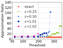
(a) facebook, r1

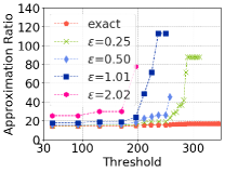
(b) facebook, r2

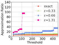
(c) GrQc, r1

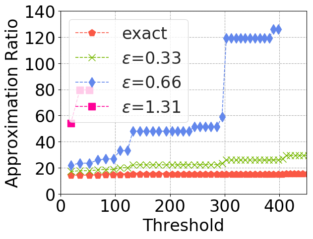
(d) GrQc, r2

Figure 3: The approximation ratios of Theorem 1 (r1) and an upper bound on that of Theorem 2 (r2) at thresholds indicated by the markers.

In order to have value oracle access to $f$ in the IT problem, the instances $G_{1},...,G_{N}$ must be stored. In addition, to compute $f(X)$ for $X\subseteq V$ the reachable vertices from $X$ must be computed for each of the $N$ instances. If $N$ is large, this is not scalable to large influence instances Cohen et al. (2014).

Motivated by this, Cohen et al. (2014) proposed using an approximate average reachability oracle in place of $f$ that is based on bottom-$k$ min-hash sketches Cohen (1997). Given $k\in\mathbb{Z}_{>0}$, the approximate average reachability oracle $F$ is constructed as follows: For every vertex, instance pair $(v,i)\in V\times\{1,...,N\}$ a random rank value $r_{v}^{i}$ is drawn from the uniform distribution on $[0,1]$. For every vertex $u\in V$, the combined reachability sketch $X_{u}$ of $u$ is the smallest $k$ values from the set $\{r_{v}^{i}:v\text{ is reachable from }u\text{ on instance }G_{i}\}$. $X_{u}$ is stored for all $u\in V$. Note that generating $X_{u}$ for all $u\in V$ does not require all the instances $G_{1},...,G_{N}$ to be stored at the same time.

Let $X\subseteq S$. If $|\cup_{u\in X}X_{u}|<k$, then $F(X)=|\cup_{u\in X}X_{u}|/N$. Otherwise, let $t$ be the $k$-th smallest value in $\cup_{u\in X}X_{u}$. Then $F(X)=(k-1)/(Nt)$.

$F$ can be made an $\epsilon$-approximation to $f$ by choosing sufficiently large $k$: For $c>2$, if $k=c\epsilon^{-2}\log(n)$ then the relative error of all queries over the duration of the greedy algorithm is within $\epsilon$ with probability at least $1-1/n^{c-2}$ Cohen et al. (2014). The relative error can be converted to absolute error as described in Section 1.3.

Proposition 1.

The approximate average reachability oracle of Cohen et al. is non-submodular.

Proof.

Consider an instance of IT where $V=\{x,y,z\}$ and three instances $G_{1},G_{2},G_{3}$ are as depicted in Figure 1.

Suppose that we construct the approximate reachability oracle of Cohen et al. with $k=5$, and the randomly generated mapping from vertex, instance pairs to the interval $[0,1]$ is as depicted in Figure 2. Then $X_{x}=\{r_{z}^{2},r_{x}^{2},r_{z}^{1},r_{y}^{1},r_{x}^{1}\}$, $X_{y}=\{r_{z}^{1},r_{y}^{3},r_{y}^{2},r_{y}^{1},r_{x}^{1}\}$, and $X_{z}=\{r_{z}^{2},r_{x}^{2},r_{z}^{1},r_{z}^{3},r_{y}^{1}\}$.

Consider adding $z$ to the sets $A=\{x\}$ and $B=\{x,y\}$. Then

$$\Delta F(A,z) =(k-1)/(3r_{y}^{1})-(k-1)/(3r_{x}^{1}),$$

$$\Delta F(B,z) =(k-1)/(3r_{y}^{3})-(k-1)/(3r_{y}^{2}).$$

If $r_{y}^{1}\approx r_{x}^{1}$, but $r_{y}^{3}$ is sufficiently smaller than $r_{y}^{2}$, $\Delta F(A,z)<\Delta F(B,z)$ despite $A\subseteq B$. ∎

The effectiveness of the approximate reachability oracle of Cohen et al. has been extensively evaluated for both IM Cohen et al. (2014) as well as IT Kuhnle et al. (2017), both with uniform cost. In particular, the approximate reachability oracle of Cohen et al. was demonstrated to be significantly faster than alternative approaches such as TIM Tang et al. (2014).

Experimental Setup

We use two real social networks: the Facebook ego network Leskovec and Mcauley (2012), and the ArXiV General Relativity collaboration network Leskovec et al. (2007), which we refer to as GrQc. Influence propagation follows the Independent Cascade (IC) model Kempe et al. (2003). The average reachability oracle, $f$, is over random realizations of the influence graph. The approximate average reachability oracle of Cohen et al., $F$, is computed over these realizations with various oracle errors $\epsilon$ and the greedy algorithm is run using these oracles. For comparison, we also run the greedy algorithm with $f$.

For the cost function, we choose a cost $c_{v}$ for each $v\in V$ by sampling from a normal distribution and then define $c(X)=\sum_{x\in X}c_{x}$. We include additional experiments with non-modular cost functions in Appendix D. Additional details about the experimental setup can be found in Appendix D.

Approximation Ratio of the Greedy Algorithm

As we described in Section 2.1, if the minimum marginal gain of any element added to the greedy solution is sufficiently large then Theorems 1 and 2 are approximation ratios.

For each run of the greedy algorithm with the approximate oracle $F$ where the minimum marginal gain was sufficiently large, we compute the ratio of Theorem 1 exactly by querying $f$ (“r1”, Figures 3(a) and 3(c)) and we compute an upper bound on the ratio of Theorem 2 with only $F$ using the argument described in the discussion of Theorem 2 (“r2”, Figures 3(b) and 3(d)). Details of how we selected $\gamma$ for the ratio of Theorem 2 can be found in Appendix D. We were generally unable to compute an upper bound on the ratio presented in Theorem 1 with just an oracle to $F$ because the $\beta$ term was too small.

In addition, we ran the greedy algorithm for the exact oracle $f$ and computed the ratios of Theorem 1 and Theorem 2 exactly where $\epsilon=0$. Note that the ratio of Theorem 1 when $\epsilon=0$ reduces to the approximation ratio for SCSC given by Soma and Yoshida (2015).

Results

The approximation ratios on the Facebook dataset are plotted in Figures 3(a) and 3(b). A marker indicates the threshold $\tau$ given as input to the greedy algorithm, and the corresponding ratio for that run. We chose the $F$ values at each step of the greedy algorithm to be the thresholds. If the minimum marginal gain of a run was too small relative to $\epsilon$ for a threshold, or the approximation was greater than 140, then no marker is plotted.

As expected, smaller oracle error $\epsilon$ implies better approximation ratios. For the same $\epsilon$, the ratio of Theorem 1 is better than the upper bound on the ratio of Theorem 2. But, recall that the latter can be computed only querying $F$. As the threshold increases, the ratio degrades because elements with smaller marginal gain are being added into the solution set, although the effect is smaller with smaller $\epsilon$.

Qualitatively similar results are shown for the GrQc dataset in Fig. 3(c) and 3(d). The ratios degrade less quickly in GrQc compared to Facebook: this is because in Facebook there are a few vertices that can be selected with high marginal gain, and then after that the marginal gains quickly decrease. In contrast, the marginal gains for GrQc are more sustained over the course of the greedy algorithm.

4 Acknowledgements

This work was supported in part by NSF CNS-1814614, NSF EFRI 1441231, and DTRA HDTRA1-14-1-0055. Victoria G. Crawford was supported by a Harris Corporation Fellowship. We thank the anonymous reviewers for their helpful feedback.

Appendix A Additional Approximation Results

A.1 The case of monotone submodular $F$

The main difficulty in proving Theorems 1 and 2 in Section 2.1 is that the $\epsilon$-approximate oracle $F$ is not monotone submodular. In the event that $F$ is monotone submodular, existing results for SCSC Wolsey [1982], Wan et al. [2010], Soma and Yoshida [2015] can be translated into results for SCSC with an $\epsilon$-approximate oracle, as the following proposition shows.

Proposition 2.

Let $\mathcal{A}$ be a bicriteria approximation algorithm for SCSC that takes as input $f,c,\tau$ and has approximation ratio $\alpha$, and feasibility guarantee $\tau-\delta$.

Suppose that we have two instances of SCSC: instance $\mathcal{I}_{1}$ with $f,c,\tau$ and instance $\mathcal{I}_{2}$ with $F,c,\tau-\epsilon$ where $F$ is an $\epsilon$-approximation to $f$. Then if we run $\mathcal{A}$ for $\mathcal{I}_{2}$ and $\mathcal{A}$ returns the set $A$, it is guaranteed that $c(A)\leq\alpha c(A^{*})$ and $f(A)\geq\tau-2\epsilon-\delta$ where $A^{*}$ is the optimal solution to instance $\mathcal{I}_{1}$.

Proof.

$A^{*}$ is a feasible solution to $\mathcal{I}_{2}$ since $F(A^{*})\geq f(A^{*})-\epsilon\geq\tau-\epsilon.$ Therefore $\alpha c(A^{*})\geq c(A)$. For the feasibility, we have that $f(A)\geq F(A)-\epsilon\geq\tau-2\epsilon-\delta.$ ∎

A.2 An alternative version of Theorem 1

The definitions and notation used in this section can be found in Section 1.3 of the paper.

The version of Theorem 1 in Section 2 requires that $\epsilon$ be small relative to the minimum marginal gain of an element added to the greedy set, $\mu$, over the duration of Algorithm 1. In particular, $\mu>4\epsilon c_{max}\rho/c_{min}$. Alternatively, we may ensure the approximation ratio of Theorem 1 if $\epsilon$ is sufficiently small by exiting Algorithm 1 if $F_{\tau}(A_{i})-F_{\tau}(A_{i-1})$ falls below an input value, $\mu^{*}$. The feasibility guarantee is weakened since Algorithm 1 does not necessarily run to completion, but not by much if $\epsilon$ is sufficiently small. In particular, we have the following alternative version of Theorem 1.

Theorem 1 (Alternative)

Suppose we have an instance of SCSC with $n\geq 1$. Let $F$ be a function that is $\epsilon$-approximate to $f$.

Let $\mu^{*}>0$ be given. Suppose Algorithm 1 is run with input $F$, $c$, and $\tau$, but we exit the algorithm at the first iteration $k$ such that $F_{\tau}(A_{k})-F_{\tau}(A_{k-1})\leq\mu^{*}$ and return $A=A_{k-1}$. Then $f(A)\geq\tau-n((c_{max}/c_{min})\mu^{*}+2\epsilon)$ and if $\epsilon<\mu^{*}/(4c_{max}\rho/c_{min}+2)$, then

$$c(A)\leq \frac{\rho}{1-\frac{4\epsilon c_{max}\rho}{c_{min}(\mu^{*}-2\epsilon)}}\left(\ln\left(\frac{\alpha}{\beta}\right)+2\right)c(A^{*})$$

where $A^{*}$ is the optimal solution to the instance of SCSC.

Proof of Theorem 1 (Alternative)

Without loss of generality we re-define $f=\min\{f,\tau\}$ and $F=\min\{F,\tau\}$. This way, $f=f_{\tau}$ and $F=F_{\tau}$.

First, we prove the feasibility. If Algorithm 1 runs to completion, then the feasibility guarantee is clear since $f(A)\geq\tau-\epsilon$. Suppose that Algorithm 1 did not run to completion, but instead returned $A=A_{k-1}$ once $F(A_{k})-F(A_{k-1})\leq\mu^{*}$. Let $x_{k}$ be the element that is selected in the $k$th iteration. Then for all $x$

$$\Delta F(A,x)\leq\frac{c(x)}{c(x_{k})}\Delta F(A,x_{k})\leq\frac{c_{max}}{c_{min}}\mu^{*}.$$

Therefore for all $x$ $\Delta f(A,x)\leq\Delta F(A,x)+2\epsilon\leq(c_{max}/c_{min})\mu^{*}+2\epsilon$. By the submodularity of $f$ we have that

$$\tau-f(A)\leq f(S)-f(A)\leq\sum_{x}\Delta f(A,x)\leq n\left(\frac{c_{max}}{c_{min}}\mu^{*}+2\epsilon\right)$$

and so the feasibility guarantee is proven.

The approximation ratio follows by using the same argument as in Theorem 1 where $\mu$ is replaced by $\mu^{*}-2\epsilon$ since

$$\mu=\min\{f(A_{i})-f(A_{i-1}):i\leq k\}\geq\min\{F(A_{i})-F(A_{i-1}):i\leq k\}-2\epsilon>\mu^{*}-2\epsilon.$$

∎

Appendix B Proof of Theorem 1

The definitions and notation used in this section can be found in Section 1.3 of the paper.

Theorem 1

Suppose we have an instance of SCSC. Let $F$ be a function that is $\epsilon$-approximate to $f$.

Suppose we run Algorithm 1 with input $F$, $c$, and $\tau$. Then $f(A)\geq\tau-\epsilon$. And if $\mu>4\epsilon c_{max}\rho/c_{min}$,

$$c(A)\leq \frac{\rho}{1-\frac{4\epsilon c_{max}\rho}{c_{min}\mu}}\left(\ln\left(\frac{\alpha}{\beta}\right)+2\right)c(A^{*})$$

where $A^{*}$ is an optimal solution to the instance of SCSC.

Proof of Theorem 1

The feasibility guarantee is clear from the stopping condition on the greedy algorithm: $f(A)\geq F(A)-\epsilon\geq\tau-\epsilon$.

We now prove the upper bound on $c(A)$ if $\mu>4\epsilon c_{max}\rho/c_{min}$. Without loss of generality we re-define $f=\min\{f,\tau\}$ and $F=\min\{F,\tau\}$. This way, $f=f_{\tau}$ and $F=F_{\tau}$. Notice that this does not change that $F$ is an $\epsilon$-approximation of $f$ since the error is absolute.

Let $x_{1},...,x_{k}$ be the elements of $A$ in the order that they were chosen by the greedy algorithm. If $k=0$, then $c(A)=0$ and the approximation ratio is clear. For the rest of the proof, we assume that $k\geq 1$.

We define a sequence of elements $\tilde{x}_{1},...,\tilde{x}_{k}$ where

$$\tilde{x}_{i}=\text{argmax}_{x\in S\setminus A_{i-1}}\frac{\Delta f(A_{i-1},x)}{c(x)}.$$

$\tilde{x}_{i}$ has the most cost-effective marginal gain of being added to $A_{i-1}$ according to $f$, while $x_{i}$ has the most cost-effective marginal gain of being added to $A_{i-1}$ according to $F$. Note that the same element can appear multiple times in the sequence $\tilde{x}_{1},...,\tilde{x}_{k}$. In addition, we have a lower bound on $\Delta f(A_{i-1},\tilde{x}_{i})$:

$$\Delta f(A_{i-1},\tilde{x}_{i})\geq\frac{c(\tilde{x}_{i})}{c(x_{i})}\Delta f(A_{i-1},x_{i})\geq\frac{c_{min}}{c_{max}}\mu.$$ (1)

Our argument to bound $c(A)$ will follow the following three steps: (a) We bound $c(A)$ in terms of the costs of the elements $\tilde{x}_{1},...,\tilde{x}_{k}$. (b) We charge the elements of $A^{*}$ with the costs of the elements $\tilde{x}_{1},...,\tilde{x}_{k}$, and bound $c(A)$ in terms of the total charge on all elements in $A^{*}$. (c) We bound the total charge on the elements of $A^{*}$ in terms of $c(A^{*})$.

(a)

First, we bound $c(A)$ in terms of the costs of the elements $\tilde{x}_{1},...,\tilde{x}_{k}$. At iteration $i$ of Algorithm 1, the most cost-effective element to add to the set $A_{i-1}$ according to $F$ is $x_{i}$. Using the fact that $F$ is $\epsilon$-approximate to $f$, we can bound how much more cost-effective $\tilde{x}_{i}$ is compared to $x_{i}$ according to $f$ as follows:

$$\frac{\Delta f(A_{i-1},x_{i})+2\epsilon}{c(x_{i})}\geq\frac{\Delta F(A_{i-1},x_{i})}{c(x_{i})}\geq\frac{\Delta F(A_{i-1},\tilde{x}_{i})}{c(\tilde{x}_{i})}\geq\frac{\Delta f(A_{i-1},\tilde{x}_{i})-2\epsilon}{c(\tilde{x}_{i})}$$

which implies that

$$\frac{\Delta f(A_{i-1},x_{i})}{c(x_{i})}+\frac{2\epsilon(c(x_{i})+c(\tilde{x}_{i}))}{c(x_{i})c(\tilde{x}_{i})}\geq\frac{\Delta f(A_{i-1},\tilde{x}_{i})}{c(\tilde{x}_{i})}.$$ (2)

$\Delta f(A_{i-1},x_{i})\geq\mu>0$ by assumption, and $\Delta f(A_{i-1},\tilde{x}_{i})\geq(c_{min}/c_{max})\mu>0$ by Equation (1). Therefore we can re-arrange Equation (2) to be

$$\frac{c(\tilde{x}_{i})}{\Delta f(A_{i-1},\tilde{x}_{i})}+\alpha_{i}\geq\frac{c(x_{i})}{\Delta f(A_{i-1},x_{i})}\text{, where }\alpha_{i}=\frac{2\epsilon(c(x_{i})+c(\tilde{x}_{i}))}{\Delta f(A_{i-1},\tilde{x}_{i})\Delta f(A_{i-1},x_{i})}.$$ (3)

Inequality (3) and the submodularity of $c$ imply that

$$c(A) \leq\sum_{i=1}^{k}c(x_{i})=\sum_{i=1}^{k}\Delta f(A_{i-1},x_{i})\frac{c(x_{i})}{\Delta f(A_{i-1},x_{i})}$$

$$\leq\sum_{i=1}^{k}\Delta f(A_{i-1},{x_{i}})\left(\frac{c(\tilde{x}_{i})}{\Delta f(A_{i-1},\tilde{x}_{i})}+\alpha_{i}\right)$$

$$=\sum_{i=1}^{k}\Delta f(A_{i-1},x_{i})\frac{c(\tilde{x}_{i})}{\Delta f(A_{i-1},\tilde{x}_{i})}+\sum_{i=1}^{k}\frac{2\epsilon(c(\tilde{x}_{i})+c(x_{i}))}{\Delta f(A_{i-1},\tilde{x}_{i})}.$$ (4)

We now bound the second term on the right side of Equation (4) by

$$\sum_{i=1}^{k}\frac{2\epsilon(c(\tilde{x}_{i})+c(x_{i}))}{\Delta f(A_{i-1},\tilde{x}_{i})} =\sum_{i=1}^{k}\frac{2\epsilon c(\tilde{x}_{i})}{\Delta f(A_{i-1},\tilde{x}_{i})}+\sum_{i=1}^{k}\frac{2\epsilon c(x_{i})}{\Delta f(A_{i-1},\tilde{x}_{i})}$$

$$\leq\sum_{i=1}^{k}\frac{2\epsilon c(x_{i})}{\Delta f(A_{i-1},x_{i})}+\sum_{i=1}^{k}\frac{2\epsilon c(x_{i})}{\Delta f(A_{i-1},\tilde{x}_{i})}$$

$$\leq\frac{4\epsilon c_{max}}{c_{min}\mu}\sum_{i=1}^{k}c(x_{i})$$

$$\leq\frac{4\epsilon c_{max}\rho}{c_{min}\mu}c(A).$$ (5)

The second to last inequality in Equation (5) follows from the fact that $\Delta f(A_{i-1},x_{i})\geq\mu\geq(c_{min}/c_{max})\mu$, and that by Equation (1) $\Delta f(A_{i-1},\tilde{x}_{i})\geq(c_{min}/c_{max})\mu$. The last inequality in Equation (5) uses the definition of the curvature $\rho$ of $c$.

Combining Equations (4) and (5) gives us the following bound on $c(A)$ in terms of the costs of the elements $\tilde{x}_{1},...,\tilde{x}_{k}$:

$$\left(1-\frac{4\epsilon c_{max}\rho}{c_{min}\mu}\right)c(A)\leq\sum_{i=1}^{k}\frac{\Delta f(A_{i-1},x_{i})}{\Delta f(A_{i-1},\tilde{x}_{i})}c(\tilde{x}_{i}).$$ (6)

(b)

Next, we charge the elements of $A^{*}$ with the costs of the elements $\tilde{x}_{1},...,\tilde{x}_{k}$, and bound $c(A)$ in terms of the total charge on all elements in $A^{*}$. By this we mean that we give each $y\in A^{*}$ a portion of the total cost of the elements $\tilde{x}_{1},...,\tilde{x}_{k}$. In particular, we give each $y\in A^{*}$ a charge of $w(y)$, defined by

$$w(y)=\sum_{i=1}^{k}(\pi_{i}(y)-\pi_{i+1}(y))\omega_{i}\text{, where }\omega_{i}=\frac{c(\tilde{x}_{i})}{\Delta f(A_{i-1},\tilde{x}_{i})},\text{ and }\pi_{i}(y)=\begin{cases}\Delta f(A_{i-1},y)&i\in\{1,...,k\}\\ \Delta f(A,y)&i=k+1\end{cases}.$$

Recall that $\Delta f(A_{i-1},\tilde{x}_{i})>0$ for all $i$ by Equation (1), and so we can define $\omega_{i}$ as above. Wan et al. charged the elements of $A^{*}$ with the cost of elements $x_{1},...,x_{k}$ analogously to the above. We charge with the cost of elements $\tilde{x}_{1},...,\tilde{x}_{k}$ because they exhibit diminishing cost-effectiveness, i.e. $\omega_{i}-\omega_{i-1}\geq 0$ for all $i\in\{1,...,k\}$, which is needed to proceed with the argument. Because we choose $x_{1},...,x_{k}$ with $F$, which is not monotone submodular, $x_{1},...,x_{k}$ do not exhibit diminishing cost-effectiveness even if we replace $f$ with $F$ in the definition of $w(y)$ above. We now follow an argument analogous to Wan et al. but with the elements $\tilde{x}_{1},...,\tilde{x}_{k}$ in order to prove Equation (9).

Consider any $y\in A^{*}$. We can re-write $w(y)$ as

$$w(y) =\sum_{i=1}^{k}(\pi_{i}(y)-\pi_{i+1}(y))\omega_{i}$$

$$=\sum_{i=1}^{k}\pi_{i}(y)\omega_{i}-\sum_{i=1}^{k}\pi_{i+1}(y)\omega_{i}$$

$$=\pi_{1}(y)\omega_{1}+\sum_{i=2}^{k}\pi_{i}(y)\omega_{i}-\sum_{i=2}^{k}\pi_{i}(y)\omega_{i-1}-\pi_{k+1}(y)\omega_{k}$$

$$=\pi_{1}(y)\omega_{1}-\Delta f(A,y)\omega_{k}+\sum_{i=2}^{k}(\omega_{i}-\omega_{i-1})\pi_{i}(y).$$

Summing over $y\in A^{*}$, we have

$$\sum_{y\in A^{*}}w(y) =\omega_{1}\sum_{y\in A^{*}}\pi_{1}(y)+\sum_{i=2}^{k}(\omega_{i}-\omega_{i-1})\sum_{y\in A^{*}}\pi_{i}(y)-\sum_{y\in A^{*}}\Delta f(A,y)\omega_{k}.$$ (7)

On the other hand, starting with Equation (6), we see that

$$\left(1-\frac{4\epsilon c_{max}\rho}{\mu c_{min}}\right)c(A) \leq\sum_{i=1}^{k}\frac{\Delta f(A_{i-1},x_{i})}{\Delta f(A_{i-1},\tilde{x}_{i})}c(\tilde{x}_{i})$$

$$=\Delta f(A_{k-1},x_{k})\omega_{k}+\sum_{i=1}^{k-1}\Delta f(A_{i-1},x_{i})\omega_{i}$$

$$=\Delta f(A_{k-1},x_{k})\omega_{k}+\sum_{i=1}^{k-1}(\sum_{j=i}^{k}\Delta f(A_{j-1},x_{j})-\sum_{j=i+1}^{k}\Delta f(A_{j-1},x_{j}))\omega_{i}$$

$$=\sum_{i=1}^{k}\sum_{j=i}^{k}\Delta f(A_{j-1},x_{j})\omega_{i}-\sum_{i=1}^{k-1}\sum_{j=i+1}^{k}\Delta f(A_{j-1},x_{j})\omega_{i}$$

$$=\omega_{1}\sum_{j=1}^{k}\Delta f(A_{j-1},x_{j})+\sum_{i=2}^{k}\sum_{j=i}^{k}\Delta f(A_{j-1},x_{j})\omega_{i}-\sum_{i=2}^{k}\sum_{j=i}^{k}\Delta f(A_{j-1},x_{j})\omega_{i-1}$$

$$=\omega_{1}\sum_{j=1}^{k}\Delta f(A_{j-1},x_{j})+\sum_{i=2}^{k}(\omega_{i}-\omega_{i-1})\sum_{j=i}^{k}\Delta f(A_{j-1},x_{j}).$$ (8)

In order to find a link between Equations (7) and (8), we first notice that for any $i\in\{1,...,k\}$

$$\sum_{j=i}^{k}\Delta f(A_{j-1},x_{j})=f(A_{k})-f(A_{i-1})\leq\sum_{y\in A^{*}}\Delta f(A_{i-1},y)=\sum_{y\in A^{*}}\pi_{i}(y).$$

In addition, for any $i\in\{1,...,k\}$

$$\omega_{i}-\omega_{i-1} =\frac{c(\tilde{x}_{i})}{\Delta f(A_{i-1},\tilde{x}_{i})}-\frac{c(\tilde{x}_{i-1})}{\Delta f(A_{i-2},\tilde{x}_{i-1})}$$

$$\geq\frac{c(\tilde{x}_{i})}{\Delta f(A_{i-2},\tilde{x}_{i})}-\frac{c(\tilde{x}_{i-1})}{\Delta f(A_{i-2},\tilde{x}_{i-1})}$$

$$\geq\frac{c(\tilde{x}_{i-1})}{\Delta f(A_{i-2},\tilde{x}_{i-1})}-\frac{c(\tilde{x}_{i-1})}{\Delta f(A_{i-2},\tilde{x}_{i-1})}=0.$$

We may therefore link Equations (7) and (8) to see that

$$\left(1-\frac{4\epsilon c_{max}\rho}{\mu c_{min}}\right)c(A) \leq\omega_{1}\sum_{j=1}^{k}\Delta f(A_{j-1},x_{j})+\sum_{i=2}^{k}(\omega_{i}-\omega_{i-1})\sum_{j=i}^{k}\Delta f(A_{j-1},x_{j})$$

$$\leq\sum_{y\in A^{*}}w(y)+\sum_{y\in A^{*}}\Delta f(A,y)\omega_{k}.$$ (9)

Consider $y\in A^{*}$. $f(A)$ is not necessarily $\tau$ since the stopping condition for Algorithm 1 is only that $F(A)\geq\tau$. In this case, if $\Delta f(A,y)\neq 0$ for $y\in A^{*}$ (which implies that $y\notin A_{k-1}$) then by the submodularity of $f$

$$\Delta f(A,y)\omega_{k}=\Delta f(A,y)\frac{c(\tilde{x}_{k})}{\Delta f(A_{k-1},\tilde{x}_{k})}\leq\Delta f(A,y)\frac{c(y)}{\Delta f(A_{k-1},y)}\leq\Delta f(A,y)\frac{c(y)}{\Delta f(A,y)}=c(y).$$

Therefore we can bound $c(A)$ in terms of the total charge on all elements in $A^{*}$:

$$\left(1-\frac{4\epsilon c_{max}\rho}{\mu c_{min}}\right)c(A)\leq\sum_{y\in A^{*}}w(y)+\sum_{y\in A^{*}}c(y)\leq\sum_{y\in A^{*}}w(y)+\rho c(A^{*}).$$ (10)

(c)

Finally, we bound the total charge on the elements of $A^{*}$ in terms of $c(A^{*})$.

We first define a value $\ell_{y}$ for every $y\in A^{*}$. For each $y\in A^{*}$, if $\pi_{1}(y)=0$ we set $\ell_{y}=0$, otherwise $\ell_{y}$ is the value in $\{1,...,k\}$ such that if $i\in\{1,...,\ell_{y}\}$ then $\pi_{i}(y)>0$, and if $i\in\{\ell_{y}+1,...,k\}$ then $\pi_{i}(y)=0$. Such an $\ell_{y}$ can be set since $f$ is submodular and monotonic. Then

$$w(y) =\sum_{i=1}^{\ell_{y}}(\pi_{i}(y)-\pi_{i+1}(y))\omega_{i}$$

$$\leq\sum_{i=1}^{\ell_{y}}(\pi_{i}(y)-\pi_{i+1}(y))\frac{c(y)}{\pi_{i}(y)}$$

$$\leq c(y)\left(\left(\sum_{i=1}^{\ell_{y}-1}\frac{\pi_{i}(y)-\pi_{i+1}(y)}{\pi_{i}(y)}\right)+1\right)$$

$$\leq c(y)\left(\sum_{i=1}^{\ell_{y}-1}(\ln(\pi_{i}(y))-\ln(\pi_{i+1}(y)))+1\right)$$

$$=c(y)\left(\ln(\pi_{1}(y))-\ln(\pi_{\ell_{y}}(y))+1\right)$$

$$\leq c(y)\left(\ln\left(\frac{\alpha}{\beta}\right)+1\right).$$ (11)

The third to last inequality follows since

$$\frac{\pi_{i}(y)-\pi_{i+1}(y)}{\pi_{i}(y)}=\int_{\pi_{i+1}(y)}^{\pi_{i}(y)}\frac{1}{\pi_{i}(y)}dx\leq\int_{\pi_{i+1}(y)}^{\pi_{i}(y)}\frac{1}{x}dx=\ln(\pi_{i}(y))-\ln(\pi_{i+1}(y)).$$

We sum inequality (11) over all $y\in A^{*}$ to get that

$$\sum_{y\in A^{*}}w(y)\leq\left(\ln\left(\frac{\alpha}{\beta}\right)+1\right)\sum_{y\in A^{*}}c(y)\leq\rho\left(\ln\left(\frac{\alpha}{\beta}\right)+1\right)c(A^{*}).$$ (12)

Finally, we combine inequality (10) and inequality (1) to see that

$$\left(1-\frac{4\epsilon c_{max}\rho}{c_{min}\mu}\right)c(A) \leq\sum_{y\in A^{*}}w(y)+\rho c(A^{*})\leq\rho\left(\ln\left(\frac{\alpha}{\beta}\right)+1\right)c(A^{*})+\rho c(A^{*}).$$

If $\mu>(4\epsilon c_{max}\rho)/(c_{min})$, this completes the proof of the approximation guarantee in the theorem statement. ∎

Appendix C Proof of Theorem 2

The definitions and notation used in this section can be found in Section 2.1 of the paper.

Theorem 2

Suppose we have an instance of SCSC. Let $F$ be a function that is $\epsilon$-approximate to $f$.

Suppose we run Algorithm 1 with input $F$, $c$, and $\tau$. Then $f(A)\geq\tau-\epsilon$. And if $\mu>4\epsilon c_{max}\rho/c_{min}$, then for any $\gamma\in\left(0,1-4\epsilon c_{max}\rho/c_{min}\mu\right)$,

$$c(A)\leq \frac{\rho}{1-\frac{4\epsilon c_{max}\rho}{c_{min}\mu}-\gamma}\left(\ln\left(\frac{n\alpha\rho}{\gamma\mu}\right)+2\right)c(A^{*})$$

where $A^{*}$ is an optimal solution to the instance of SCSC.

Proof of Theorem 2

The argument for the proof of Theorem 2 is the same as Theorem 1, except for part (c) which is what we present here. In particular, we have gotten to the point of the proof of Theorem 1 where we have proven that

$$\left(1-\frac{4\epsilon c_{max}\rho}{c_{min}\mu}\right)c(A)\leq\sum_{y\in A^{*}}w(y)+\rho c(A^{*}).$$ (1)

Let $\lambda>0$. We first define a value $m_{y}$ for every $y\in A^{*}$. For each $y\in A^{*}$, if $\pi_{1}(y)\leq\lambda$ we set $m_{y}=0$, otherwise $m_{y}$ is the value in $\{1,...,k\}$ such that if $i\in\{1,...,m_{y}\}$ then $\pi_{i}(y)>\lambda$, and if $i\in\{m_{y}+1,...,k\}$ then $\pi_{i}(y)\leq\lambda$. Such an $m_{y}$ can be set since $f$ is submodular and monotonic. Then

$$w(y)=\sum_{i=1}^{m_{y}}(\pi_{i}(y)-\pi_{i+1}(y))\omega_{i}+\sum_{i=m_{y}+1}^{k}(\pi_{i}(y)-\pi_{i+1}(y))\omega_{i}.$$ (2)

A similar analysis as in the proof of Theorem 1 can be used to show that

$$\sum_{i=1}^{m_{y}}(\pi_{i}(y)-\pi_{i+1}(y))\omega_{i}\leq c(y)\left(\ln\left(\frac{\alpha}{\lambda}\right)+1\right).$$ (3)

The remaining part of inequality (2) can be bounded by

$$\sum_{i=m_{y}+1}^{k}(\pi_{i}(y)-\pi_{i+1}(y))\omega_{i} \leq\sum_{i=m_{y}+1}^{k}(\pi_{i}(y)-\pi_{i+1}(y))\frac{c(x_{i})}{\Delta f(A_{i-1},x_{i})}$$

$$\leq\sum_{i=m_{y}+1}^{k}\pi_{i}(y)\frac{c(x_{i})}{\Delta f(A_{i-1},x_{i})}$$

$$<\sum_{i=m_{y}+1}^{k}\lambda\frac{c(x_{i})}{\mu}$$

$$\leq\frac{\lambda\rho}{\mu}c(A).$$ (4)

Summing Equation (2) over all $y\in A^{*}$ and applying the upper bounds in Equations (3) and (4) gives us that

$$\sum_{y\in A^{*}}w(y) \leq\rho\left(\ln\left(\frac{\alpha}{\lambda}\right)+1\right)c(A^{*})+\frac{\lambda\rho n}{\mu}c(A)$$ (5)

By combining Equations (5) and (1), we have that

$$\left(1-\frac{4\epsilon c_{max}\rho}{c_{min}\mu}-\frac{\lambda\rho n}{\mu}\right)c(A) \leq\rho\left(\ln\left(\frac{\alpha}{\lambda}\right)+2\right)c(A^{*}).$$

If we set $\lambda=(\gamma\mu)/(n\rho)$ we have the approximation ratio in the theorem statement. ∎

Appendix D Application and Experiments

Influence Threshold (IT) (Non-Simulation)

In contrast to the version of IT in Section 3 of the paper, we may define IT to directly use the influence model as follows.

Let $G=(V,E)$ be a social network where nodes $V$ represents users, edges $E$ represent social connections, and $\mathcal{D}$ is a probability distribution over subsets of $E$ that represents the probability of a set of edges being “alive”. Activation of users in the social network starts from an initial seed set and then propagates across alive edges. For $X\subseteq S$, $f(X)$ is the expected number of reachable nodes in $V$ from $X$ when a set of alive edges is sampled from $\mathcal{D}$. $c:2^{V}\to\mathbb{R}_{\geq 0}$ is a monotone submodular function that gives the cost of seeding a set of users. The Influence Threshold problem (IT) is to find a seed set $A$ such that $c(A)$ is minimized and $f(A)\geq\tau$.

$f$ as Average Reachability

One popular choice for the distribution $\mathcal{D}$ is the Independent Cascade (IC) model Kempe et al. [2003]. In the IC model, every edge has a probability assigned to it $w_{E}:E\to[0,1]$. Each edge $e$ is independently alive with probability $w_{E}(e)$. However, computing the expected influence $f$ under the IC model is $\#P$-hard and therefore impractical to compute Chen et al. [2010].

As an alternative to working directly with the influence model Kempe et al. proposed a simulation-based approach to approximating it: Random samples from $\mathcal{D}$ are drawn, and for every $X\subseteq S$ $f(X)$ is approximated by the average number of reachable nodes from $X$ over the samples. The resulting approximation of $f$ is unbiased, converges to the expected value, and is monotone submodular. This simulation-based approach is also advantageous since it can be used for more complex models than IC or for instances generated from traces Cohen et al. [2014].

Because the average reachability is monotone submodular, it is easy to translate approximation results for IT where $f$ is replaced by the average reachability into approximation results for IT (see Proposition 2 of Appendix A).

Additional Experimental Setup Details

We use two real social networks: the Facebook ego network Leskovec and Mcauley [2012] with $n=4039$, and the ArXiV General Relativity collaboration network with $n=5242$ Leskovec et al. [2007], which we refer to as GrQc.

Influence propagation follows the Independent Cascade (IC) model Kempe et al. [2003]. The probabilities assigned to the edges $w_{E}:E\to[0,1]$ follow the weighted cascade model Kempe et al. [2003]. In the weighted cascade model, an edge that goes from $u\in V$ to $v\in V$ is assigned probability $\frac{q}{d_{v}}$ where $d_{v}$ is the number of incoming edges to node $v$ and $q\in(0,1]$. For facebook $q=0.5$, and for GrQc $q=0.8$.

The average reachability oracle, $f$, is over $N=25000$ random realizations of the influence graph. The approximate average reachability oracle of Cohen et al., $F$, is computed over these realizations with various oracle errors $\epsilon$ and the greedy algorithm is run using these oracles. For comparison, we also run the greedy algorithm with $f$.

For the cost function $c:2^{V}\to\mathbb{R}_{\geq 0}$, we choose a cost $c_{v}$ for each $v\in V$ by sampling from a normal distribution with mean 1 and standard deviation 0.1, and then define $c(X)=\sum_{x\in X}c_{x}$.

To select the parameter $\gamma$ when computing the ratio of Theorem 2, we discretize the domain of $\gamma$, compute the ratio on each of the points, and select the $\gamma$ that gives the smallest approximation ratio.

Additional Experimental Results

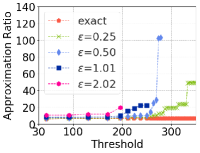
(a) facebook, r1, $\rho=1.0$

(b) facebook, r1, $\rho=1.2$

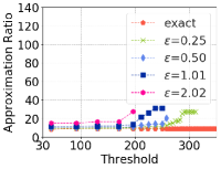
(c) facebook, r1, $\rho=1.4$

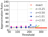
(d) facebook, r1, $\rho=1.6$

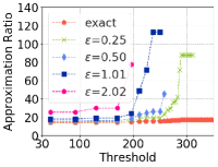
(e) facebook, r2, $\rho=1.0$

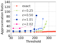
(f) facebook, r2, $\rho=1.2$

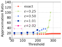
(g) facebook, r2, $\rho=1.4$

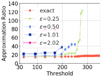
(h) facebook, r2, $\rho=1.6$

Figure 4: The approximation ratios of Theorem 1 (r1) and an upper bound on that of Theorem 2 (r2) at thresholds indicated by the markers.

The experimental results presented in Section 3 of the paper consider a modular cost function. However, the approximation results presented in Theorems 1 and 2 are for general submodular cost functions. In this section, we present additional experimental results analogous to those in Section 3 of the paper but with non-modular cost function.

Recall from Section 1.3 that a measure of how far a function is from being is modular is measured by its curvature, $\rho\in[1,\infty)$. Our approximation ratios in Theorems 1 and 2 depend on $\rho$: the smaller $\rho$, and hence the closer to being modular the function is, the better the approximation ratio.

Notice that the greedy algorithm, presented in Section 1.3, chooses elements only according to singleton costs. Therefore, the experimental results in Section 3 of the paper can easily be extended to cost functions that are not modular by simply computing the ratio for different values of cost curvature, $\rho$; higher values of $\rho$ would require smaller epsilon to get the same ratio.

The approximation ratio of Theorem 1 on the Facebook dataset is plotted in Figures 4(a) to 4(d) for varying curvature $\rho$, and that of Theorem 2 is plotted in Figures 4(e) to 4(h). As $\rho$ increases, the approximation ratios are subtly greater. The greater that $\rho$ is, the greater $\mu$ must be relative to $\epsilon$ in order to have the approximation ratios of Theorems 1 and 2. This results in the ratios of Theorems 1 and 2 not being guaranteed at lower thresholds for larger $\rho$.

References

- Badanidiyuru et al. (2012) A. Badanidiyuru, S. Dobzinski, H. Fu, R. Kleinberg, N. Nisan, and T. Roughgarden. Sketching valuation functions. In Proceedings of the twenty-third annual ACM-SIAM symposium on Discrete Algorithms, pages 1025–1035. Society for Industrial and Applied Mathematics, 2012.
- Balcan et al. (2012) M. F. Balcan, F. Constantin, S. Iwata, and L. Wang. Learning valuation functions. In Conference on Learning Theory, pages 4–1, 2012.
- Bian et al. (2017) A. A. Bian, J. M. Buhmann, A. Krause, and S. Tschiatschek. Guarantees for Greedy Maximization of Non-submodular Functions with Applications. In Proceedings of the 34th International Conference on Machine Learning (ICML), 2017.
- Chen et al. (2018) L. Chen, M. Feldman, and A. Karbasi. Weakly Submodular Maximization Beyond Cardinality Constraints: Does Randomization Help Greedy? In International Conference on Machine Learning (ICML), 2018. URL http://arxiv.org/abs/1707.04347.
- Chen et al. (2010) W. Chen, C. Wang, and Y. Wang. Scalable influence maximization for prevalent viral marketing in large-scale social networks. In Proceedings of the 16th ACM SIGKDD international conference on Knowledge discovery and data mining, pages 1029–1038. ACM, 2010.
- Chen et al. (2015) Y. Chen, S. H. Hassani, A. Karbasi, and A. Krause. Sequential information maximization: When is greedy near-optimal? In Conference on Learning Theory, pages 338–363, 2015.
- Cohen (1997) E. Cohen. Size-estimation framework with applications to transitive closure and reachability. Journal of Computer and System Sciences, 55(3):441–453, 1997.
- Cohen et al. (2014) E. Cohen, D. Delling, T. Pajor, and R. F. Werneck. Sketch-based influence maximization and computation: Scaling up with guarantees. In Proceedings of the 23rd ACM International Conference on Conference on Information and Knowledge Management, pages 629–638. ACM, 2014.
- Dinh et al. (2014) T. N. Dinh, H. Zhang, D. T. Nguyen, and M. T. Thai. Cost-effective viral marketing for time-critical campaigns in large-scale social networks. IEEE/ACM Transactions on Networking (ToN), 22(6):2001–2011, 2014.
- Feige (1998) U. Feige. A threshold of ln n for approximating set cover. Journal of the ACM (JACM), 45(4):634–652, 1998.
- Goyal et al. (2013) A. Goyal, F. Bonchi, L. V. Lakshmanan, and S. Venkatasubramanian. On minimizing budget and time in influence propagation over social networks. Social network analysis and mining, 3(2):179–192, 2013.
- Guillory and Bilmes (2011) A. Guillory and J. A. Bilmes. Simultaneous learning and covering with adversarial noise. In ICML, volume 11, pages 369–376, 2011.
- Han et al. (2017) K. Han, Y. He, S. Tang, H. Huang, and C. Xu. Cost-effective seed selection in online social networks. arXiv preprint arXiv:1711.10665, 2017.
- Hassidim and Singer (2017) A. Hassidim and Y. Singer. Submodular optimization under noise. In Conference on Learning Theory, pages 1069–1122, 2017.
- He et al. (2014) J. S. He, S. Ji, R. Beyah, and Z. Cai. Minimum-sized influential node set selection for social networks under the independent cascade model. In Proceedings of the 15th ACM International Symposium on Mobile ad hoc Networking and Computing, pages 93–102. ACM, 2014.
- Horel and Singer (2016) T. Horel and Y. Singer. Maximization of approximately submodular functions. In Advances in Neural Information Processing Systems, pages 3045–3053, 2016.
- Iyer and Bilmes (2013) R. K. Iyer and J. A. Bilmes. Submodular optimization with submodular cover and submodular knapsack constraints. In Advances in Neural Information Processing Systems, pages 2436–2444, 2013.
- Kempe et al. (2003) D. Kempe, J. Kleinberg, and É. Tardos. Maximizing the spread of influence through a social network. In Proceedings of the ninth ACM SIGKDD international conference on Knowledge discovery and data mining, pages 137–146. ACM, 2003.
- Kuhnle et al. (2017) A. Kuhnle, T. Pan, M. A. Alim, and M. T. Thai. Scalable bicriteria algorithms for the threshold activation problem in online social networks. In INFOCOM 2017-IEEE Conference on Computer Communications, IEEE, pages 1–9. IEEE, 2017.
- Kuhnle et al. (2018) A. Kuhnle, J. D. Smith, V. G. Crawford, and M. T. Thai. Fast Maximization of Non-Submodular, Monotonic Functions on the Integer Lattice. In International Conference on Machine Learning (ICML), 2018. URL http://arxiv.org/abs/1805.06990.
- Leskovec and Mcauley (2012) J. Leskovec and J. J. Mcauley. Learning to discover social circles in ego networks. In Advances in neural information processing systems, pages 539–547, 2012.
- Leskovec et al. (2007) J. Leskovec, J. Kleinberg, and C. Faloutsos. Graph evolution: Densification and shrinking diameters. ACM Transactions on Knowledge Discovery from Data (TKDD), 1(1):2, 2007.
- Li et al. (2017) X. Li, J. D. Smith, T. N. Dinh, and M. T. Thai. Why approximate when you can get the exact? optimal targeted viral marketing at scale. In IEEE INFOCOM 2017-IEEE Conference on Computer Communications, pages 1–9. IEEE, 2017.
- Lin and Bilmes (2011) H. Lin and J. Bilmes. A class of submodular functions for document summarization. In Proceedings of the 49th Annual Meeting of the Association for Computational Linguistics: Human Language Technologies-Volume 1, pages 510–520. Association for Computational Linguistics, 2011.
- Mirzasoleiman et al. (2015) B. Mirzasoleiman, A. Karbasi, A. Badanidiyuru, and A. Krause. Distributed submodular cover: Succinctly summarizing massive data. In Advances in Neural Information Processing Systems, pages 2881–2889, 2015.
- Mirzasoleiman et al. (2016) B. Mirzasoleiman, M. Zadimoghaddam, and A. Karbasi. Fast distributed submodular cover: Public-private data summarization. In Advances in Neural Information Processing Systems, pages 3594–3602, 2016.
- Nemhauser et al. (1978) G. L. Nemhauser, L. A. Wolsey, and M. L. Fisher. An analysis of approximations for maximizing submodular set functions—i. Mathematical programming, 14(1):265–294, 1978.
- Norouzi-Fard et al. (2016) A. Norouzi-Fard, A. Bazzi, I. Bogunovic, M. El Halabi, Y.-P. Hsieh, and V. Cevher. An efficient streaming algorithm for the submodular cover problem. In Advances in Neural Information Processing Systems, pages 4493–4501, 2016.
- Qian et al. (2017) C. Qian, J.-C. Shi, Y. Yu, K. Tang, and Z.-H. Zhou. Subset selection under noise. In Advances in Neural Information Processing Systems, pages 3560–3570, 2017.
- Singer and Hassidim (2018) Y. Singer and A. Hassidim. Optimization for approximate submodularity. In Advances in Neural Information Processing Systems, pages 394–405, 2018.
- Singla et al. (2016) A. Singla, S. Tschiatschek, and A. Krause. Noisy submodular maximization via adaptive sampling with applications to crowdsourced image collection summarization. In AAAI, pages 2037–2043, 2016.
- Soma and Yoshida (2015) T. Soma and Y. Yoshida. A generalization of submodular cover via the diminishing return property on the integer lattice. In Advances in Neural Information Processing Systems, pages 847–855, 2015.
- Tang et al. (2014) Y. Tang, X. Xiao, and Y. Shi. Influence maximization: Near-optimal time complexity meets practical efficiency. In Proceedings of the 2014 ACM SIGMOD international conference on Management of data, pages 75–86. ACM, 2014.
- Wan et al. (2010) P.-J. Wan, D.-Z. Du, P. Pardalos, and W. Wu. Greedy approximations for minimum submodular cover with submodular cost. Computational Optimization and Applications, 45(2):463–474, 2010.
- Wei et al. (2013) K. Wei, Y. Liu, K. Kirchhoff, and J. Bilmes. Using document summarization techniques for speech data subset selection. In Proceedings of the 2013 Conference of the North American Chapter of the Association for Computational Linguistics: Human Language Technologies, pages 721–726, 2013.
- Wolsey (1982) L. A. Wolsey. An analysis of the greedy algorithm for the submodular set covering problem. Combinatorica, 2(4):385–393, 1982.
- Zhang et al. (2016) H. Zhang, A. Kuhnle, H. Zhang, and M. T. Thai. Detecting misinformation in online social networks before it is too late. In Proceedings of the 2016 IEEE/ACM International Conference on Advances in Social Networks Analysis and Mining, pages 541–548. IEEE Press, 2016.