Optimize TSK Fuzzy Systems for Classification Problems: Mini-Batch Gradient Descent with Uniform Regularization and Batch Normalization

Abstract

Takagi-Sugeno-Kang (TSK) fuzzy systems are flexible and interpretable machine learning models; however, they may not be easily optimized when the data size is large, and/or the data dimensionality is high. This paper proposes a mini-batch gradient descent (MBGD) based algorithm to efficiently and effectively train TSK fuzzy classifiers. It integrates two novel techniques: 1) uniform regularization (UR), which forces the rules to have similar average contributions to the output, and hence to increase the generalization performance of the TSK classifier; and, 2) batch normalization (BN), which extends BN from deep neural networks to TSK fuzzy classifiers to expedite the convergence and improve the generalization performance. Experiments on 12 UCI datasets from various application domains, with varying size and dimensionality, demonstrated that UR and BN are effective individually, and integrating them can further improve the classification performance.

I Introduction

Takagi-Sugeno-Kang (TSK) fuzzy systems [1] have achieved great success in numerous applications, including both classification and regression problems. Many optimization approaches have been proposed for them.

There are generally three strategies for fine-tuning the TSK fuzzy system parameters after initialization: 1) evolutionary algorithms [2, 3]; 2) gradient descent (GD) based algorithms [4]; and, 3) GD plus least squares estimation (LSE), represented by the popular adaptive-network-based fuzzy inference system (ANFIS) [5]. However, these approaches may have challenges when the size and/or the dimensionality of the data increase. Evolutionary algorithms need to keep a large population of candidate solutions, and evaluate the fitness of each, which result in high computational cost and heavy memory requirement for big data. Traditional GD needs to compute the gradients from the entire dataset to iteratively update the model parameters, which may be very slow, or even impossible, when the data size is very large. The memory requirement and computational cost of LSE also increase rapidly when the data size and/or dimensionality increase. Additionally, as shown in [6], ANFIS may result in significant overfitting in regression problems.

Many efforts have been spent to tackling the difficulty in optimizing the TSK fuzzy systems on big and/or high-dimensional data [7, 8, 9]. Dimensionality reduction and/or feature selection are usually used to reduce the number of fuzzy partitions (rules). Traditional dimensionality reduction techniques such as principal component analysis (PCA) has been used for TSK fuzzy system optimization [10, 11]. There are also methods focusing on learning a sparse subspace of the original feature space to reduce the number of antecedents in each rule [12, 13]. Once the number of antecedents is determined, different optimization approaches can be used to tune the TSK fuzzy system on large datasets. For example, Chung et al. [9] utilized the equivalence between minimum enclosing ball and the Mamdani-Larsen fuzzy inference system to train the latter using the former. Gacto et al. [14] proposed a multi-objective evolutionary algorithm to optimize TSK fuzzy systems for high-dimensional large-scale regression problems.

Mini-batch gradient descent (MBGD) [15, 16] based optimization, which is particularly popular in deep learning, can also be a solution to training TSK fuzzy systems on large and high-dimensional datasets. In each iteration, MBGD computes the gradients from a randomly selected small batch of data, instead of the entire dataset [17]. Different batch sizes can be used, according to the trade-off among the available memory, the training speed, and the expected generalization performance. The original MBGD used a constant learning rate to update the model’s parameters [17]. Later, Sutskever et al. [18] found that adding a momentum to MBGD can improve the final training performance. However, it still needs to manually select a learning rate, and the convergence may be very slow at the beginning. Kingma and Ba [19] proposed the well-known Adam algorithm to automatically rescale the gradients to achieve adaptive and individualized learning rate for each parameter, which leads to faster convergence. However, the generalization performance of Adam may not be as good as the momentum [20]; so, Keskar and Socher [21] also tried to combine the advantages of momentum and Adam to achieve both fast convergence and good generalization. Recently, Luo et al. [22] also proposed AdaBound to improve Adam. AdaBound uses an adaptive bound for the learning rate of each parameter to force the optimizer to behave like Adam at the beginning and like stochastic GD at the end. Our very recent research [6] has found that TSK fuzzy systems can achieve better performance with AdaBound than Adam for regression problems.

Although MBGD-based optimization has many advantages, it may be easily trapped into a local-minimum, and may face the gradient vanishing problem. Many other techniques have been proposed to complement MBGD for better performance. In 2015, Ioffe and Szegedy [23] proposed the well-known batch normalization (BN) approach to accelerate the training of deep neural networks by reducing the internal covariate shift. BN normalizes the input distribution of each layer, so it also alleviates the gradient vanishing problem. It has been used almost ubiquitously in deep learning, and many variants [25, 26, 27, 28] have also been proposed.

This paper, following our previous research [6] on MBGD-based optimization of TSK fuzzy systems for regression problems, considers classification problems. We use AdaBound, as in [6], to adjust the learning rates. Additionally, we propose two novel techniques for training TSK fuzzy systems for classification problems, namely, uniform regularization (UR) and BN. Our main contributions are:

1. We introduce a novel UR term to the cross-entropy loss function in training TSK fuzzy classifiers, which forces all rules to have similar average firing levels on the entire dataset. Experiments show that UR can improve the generalization performance of TSK fuzzy classifiers.

2. We extend BN from the training of deep neural networks to the training of TSK fuzzy classifiers, and show that it can speed up the convergence in training and improve the generalization performance in testing.

3. We further integrate UR and BN, and show that the combined approach outperforms each individual ones.

The remainder of this paper is organized as follows: Section II introduces the proposed UR and BN approaches. Section III presents the experimental results to validate the performances of UR and BN. Section IV draws conclusions and points out some future research directions.

II UR and BN

This section introduces the details of the TSK fuzzy classifier under consideration, our proposed UR for regularizing the loss function, and BN for more efficient and effective training of the TSK fuzzy classifier. Python implementation of our algorithm can be downloaded at https://github.com/YuqiCui/TSK_BN_UR.

II-A The TSK Fuzzy Classifier

Let the training dataset be $\mathcal{D}=\{\bm{x}_{n},y_{n}\}_{n=1}^{N}$, in which $\bm{x}_{n}=[x_{n,1},...,x_{n,D}]^{T}\in\mathbb{R}^{D\times 1}$ is a $D$-dimensional feature vector, and $y_{n}\in\{1,2,...,C\}$ the corresponding class label for a $C$-class classification problem.

Suppose the TSK fuzzy classifier has $R$ rules, in the following form:

$$\begin{split}\textup{Rule}_{r}:~{}&\textup{IF}~{}x_{1}~{}\textup{is}~{}X_{r,1}~{}\textup{and}~{}\cdots~{}\textup{and}~{}x_{D}~{}\textup{is}~{}X_{r,D},\\ &\textup{THEN}~{}y_{r}^{1}(\bm{x})=b_{r,0}^{1}+\sum_{d=1}^{D}b_{r,d}^{1}\cdot x_{d}~{}\textup{and}\cdots\\ &\qquad\qquad\textup{and}~{}y_{r}^{C}(\bm{x})=b_{r,0}^{C}+\sum_{d=1}^{D}b_{r,d}^{C}\cdot x_{d}\end{split}$$ (1)

where $X_{r,d}$ ($r=1,...,R$; $d=1,...,D$) is the membership function (MF) for the $d$-th antecedent in the $r$-th rule, and $b_{r,0}^{c}$ and $b_{r,d}^{c}$ ($c=1,...,C$) are the consequent parameters for the $c$-th class.

Different types of MFs can be used in our algorithm, as long as they are differentiable. For simplicity, Gaussian MFs are considered in this paper, and the membership grade of $x_{d}$ on $X_{r,d}$ is:

$$\mu_{X_{r,d}}(x_{d}) =\exp\left(-\frac{(x_{d}-m_{r,d})^{2}}{2\sigma_{r,d}^{2}}\right),$$ (2)

where $m_{r,d}$ and $\sigma_{r,d}$ are the center and the standard deviation of the Gaussian MF, respectively.

The output of the TSK fuzzy classifier for the $c$-th class is:

$$y^{c}(\bm{x})=\frac{\sum_{r=1}^{R}f_{r}(\bm{x})y_{r}^{c}(\bm{x})}{\sum_{r=1}^{R}f_{r}(\bm{x})},$$ (3)

where

$$f_{r}(\bm{x})=\prod_{d=1}^{D}\mu_{X_{r,d}}(x_{d})=\textup{exp}\left(-\sum_{d=1}^{D}\frac{(x_{d}-m_{r,d})^{2}}{2\sigma_{r,d}^{2}}\right)$$ (4)

is the firing level of Rule $r$. We can also re-write (3) as:

$$y^{c}(\bm{x})=\sum_{r=1}^{R}\overline{f}_{r}(\bm{x})y_{r}^{c}(\bm{x}),$$ (5)

where

$$\overline{f}_{r}(\bm{x})=\frac{f_{r}(\bm{x})}{\sum_{i=1}^{R}f_{i}(\bm{x})}$$ (6)

is the normalized firing level of Rule $r$.

Once the output vector $\bm{y}(\bm{x})=[y^{1}(\bm{x}),...,y^{C}(\bm{x})]^{T}$ is obtained, the input $\bm{x}$ is assigned to the class with the largest $y^{c}(\bm{x})$.

To optimize the TSK fuzzy classifier, we need to fine-tune the antecedent MF parameters $m_{r,d}$ and $\sigma_{r,d}$, and the consequent parameters $b_{r,0}^{c}$ and $b_{r,d}^{c}$, where $r=1,...,R$, $d=1,...,D$, and $c=1,...,C$.

II-B Uniform Regularization (UR)

Mixture of experts (MoE) [29], which is functionally equivalent to TSK fuzzy systems [30, 31, 32], is a popular machine learning algorithm. Its model is shown in Fig. 1. It trains multiple local experts, each taking care of only a small local region of the input space. For a new input, the gating network determines the activations (weights) of the local experts, and the final output is a weighted average of the local expert outputs.

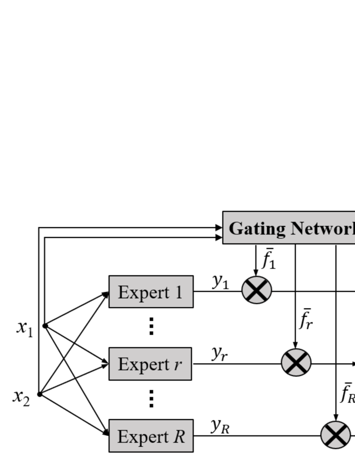
Figure 1: Mixture of experts (MoE) [29].

Although MoE has been used successfully in many applications, it may suffer from the “rich get richer” effect [33, 34]: once an expert is slightly better than others, it is always picked by the gating network, whereas other experts starve and are rarely used. This is bad for the generalization performance of the overall model.

Since MoE and TSK fuzzy systems are functionally equivalent [32], TSK fuzzy systems may also suffer from the “rich get richer” effect, i.e., only a few rules are always activated with large firing levels, whereas others have very small firing levels, and hence not adequately tuned in training. A remedy to the “rich get richer” effect in TSK fuzzy systems is to force the rules to be fired at similar degrees in the input space, so that each rule contributes about equally to the output.

Next, we propose UR to achieve this goal.

UR forces the rules to have similar average firing levels, by minimizing the following loss:

$$\ell_{UR}=\sum_{r=1}^{R}\left(\frac{1}{N}\sum_{n=1}^{N}\overline{f}_{r}(\bm{x}_{n})-\tau\right)^{2},$$ (7)

where $N$ is the number of training examples, and $\tau$ the expected firing level of each rule, which is set to $1/C$ in this paper (recall that $C$ is the number of classes).

$\ell_{UR}$ can then be added to the original loss function in MBGD-based training of TSK fuzzy classifiers, i.e., for each mini-batch with $N$ training samples,

$$\mathcal{L}=\ell+\alpha\ell_{2}+\lambda\sum_{r=1}^{R}\left(\frac{1}{N}\sum_{n=1}^{N}\overline{f}_{r}(\bm{x}_{n})-\frac{1}{R}\right)^{2},$$ (8)

where $\ell$ is the cross-entropy loss between the estimated class probabilities [obtained by applying softmax to $\bm{y}(\bm{x})$] and the true class probabilities, $\ell_{2}$ the L2 regularization of the rule consequent parameters, and $\alpha$ and $\lambda$ the trade-off parameters.

II-C Batch Normalization (BN)

BN [23] is a very powerful technique in optimizing deep neural networks [35, 36, 37]. It normalizes the data distribution in each mini-batch to accelerate the training. For a mini-batch $\mathcal{B}=\{\bm{x}_{n}\}_{n=1}^{N}$, the output of BN is [23]:

$$\bm{x}^{\prime}_{n}=BN(\bm{x}_{n})=\gamma\frac{\bm{x}_{n}-\bm{m}_{\mathcal{B}}}{\sqrt{\bm{\sigma}_{\mathcal{B}}^{2}+\epsilon}}+\beta,$$ (9)

where $\bm{m}_{\mathcal{B}}$ and $\bm{\sigma}_{\mathcal{B}}$ are the mean and the standard deviation of the samples in the mini-batch, respectively, $\gamma$ and $\beta$ are parameters to be learned during training, and $\epsilon$ is usually set to $1e-8$ to avoid being divided by zero. During training, exponential weighted averages of $\bm{m}_{\mathcal{B}}$ and $\bm{\sigma}_{\mathcal{B}}$ are recorded so that they can be used in the test phase.

Since TSK fuzzy systems and neural networks share lots of similarity [32], we can extend BN to the optimization of TSK fuzzy classifiers, as shown in Fig. 2. In the training phase, we first compute the firing level of each rule using the unmodified inputs, as in traditional TSK fuzzy systems. Then, we use BN to normalize the inputs, according to their mean and standard deviation in the current mini-batch. The normalized inputs are then used to compute the rule consequents. The final output is a weighted average of the rule consequents, the weights being the corresponding rule firing levels.

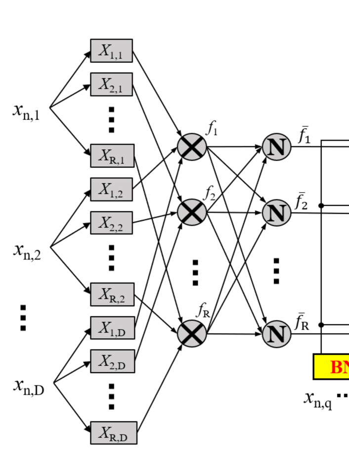
Figure 2: BN in training a TSK fuzzy classifier. All rule consequents share the same BN layer.

At the testing phase, the BN operation can be merged into the consequent layer. Assume that after training, we obtain a BN layer with learned $\bm{m}=(m_{1},...,m_{D})^{T}$, $\bm{\sigma}=(\sigma_{1},...,\sigma_{D})^{T}$, $\gamma$ and $\beta$. Then, the output $y_{r}$ of the $r$-th rule with BN is:

$$y_{r}(BN(\bm{x}_{n})) =b_{r,0}+\gamma\sum_{d=1}^{D}b_{r,d}\frac{x_{n,d}-m_{d}}{\sqrt{\sigma_{d}^{2}+\epsilon}}+\beta D,$$ (10)

which can be re-written as:

$$y_{r}(BN(\bm{x}_{n}))=b^{\prime}_{r,0}+\sum_{d=1}^{D}b^{\prime}_{r,d}x_{n,d},$$ (11)

where

$$b^{\prime}_{r,0} =b_{r,0}+\beta D-\gamma\sum_{d=1}^{D}\frac{m_{d}b_{r,d}}{\sqrt{\sigma_{d}^{2}+\epsilon}},$$ (12)

$$b^{\prime}_{r,d} =\gamma\frac{b_{r,d}}{\sqrt{\sigma_{d}^{2}+\epsilon}}.$$ (13)

By doing this, the original architecture of the TSK fuzzy classifier is kept unchanged.

We also tested two variants of BN, as shown in Fig. 3. The TSK with global BN (TSK-MBGD-UR-GBN) approach in Fig. 3 uses the BN normalized inputs in both antecedents and consequents to compute the final output. In this case, the output of TSK-MBGD-UR-GBN for Class $c$ is:

$$y^{c}(\bm{x})=\sum_{r=1}^{R}\overline{f}_{r}(BN(\bm{x}))y_{r}^{c}(BN(\bm{x})).$$ (14)

The TSK with rule-specific BN (TSK-MBGD-UR-RBN) approach in Fig. 3 uses the raw inputs to compute the antecedents, and rule-specific BN to compute each consequent individually. The output of TSK-MBGD-UR-RBN for Class $c$ is:

$$y^{c}(\bm{x})=\sum_{r=1}^{R}\overline{f}_{r}(\bm{x})y_{r}^{c}(BN_{r}(\bm{x})),$$ (15)

where $BN_{r}$ represents the BN operation for the $r$-th rule.

TSK-MBGD-UR-GBN has the same computational cost as TSK-MBGD-UR-BN, but TSK-MBGD-UR-RBN has $R$ times more BN parameters, and hence higher computational cost. Both of them can be re-expressed in the original TSK architecture. We also evaluate their performances in Section III-G.

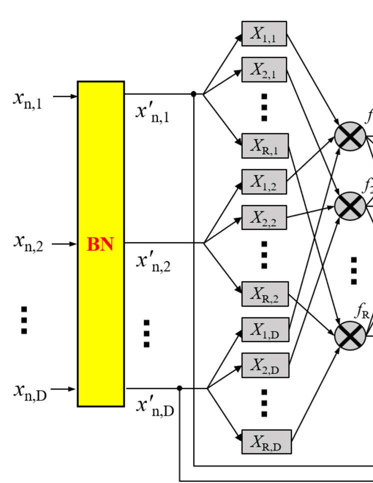
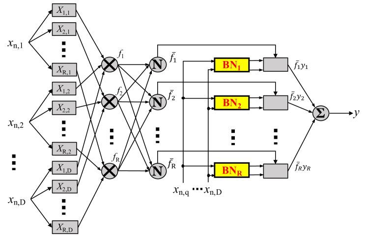
Figure 3: (a) TSK fuzzy system with global BN (TSK-MBGD-UR-GBN); and, (b) TSK fuzzy system with rule-specific BN (TSK-MBGD-UR-RBN).

III Experiments and Results

This section validates the performances of our proposed UR and BN on multiple datasets from various application domains, with varying size and feature dimensionality.

III-A Datasets

We evaluated our proposed algorithms on 12 classification datasets from the UCI Machine Learning Repository. Their characteristics are summarized in Table I. For each dataset, we randomly selected 70% samples as the training set and the remaining 30% as the test set for 30 times to get 30 different data splits. We ran each algorithm on these 30 data splits and report the average performance.

TABLE I: Summary of the 12 datasets.

Index	Dataset	No. of Samples	No. of Features	No. of Classes
1	Vehicle1	846	18	4
2	Biodeg2	1,055	41	2
3	DRD3	1151	19	2
4	Yeast4	1,484	8	10
5	Steel5	1,941	27	7
6	IS6	2,310	19	7
7	Abalone7	4,177	10	3
8	Waveform218	5,000	21	3
9	Page-blocks9	5,473	10	5
10	Satellite10	6,435	36	6
11	Clave11	10,798	16	4
12	MAGIC12	19,020	10	2

• https://archive.ics.uci.edu/ml/datasets/Statlog+%28Vehicle+Silhouettes%29

• https://archive.ics.uci.edu/ml/datasets/QSAR+biodegradation

• https://archive.ics.uci.edu/ml/datasets/Diabetic+Retinopathy+Debrecen +Data+Set

• https://archive.ics.uci.edu/ml/datasets/Yeast

• https://archive.ics.uci.edu/ml/datasets/Steel+Plates+Faults

• https://archive.ics.uci.edu/ml/datasets/Image+Segmentation

• https://archive.ics.uci.edu/ml/datasets/Abalone

• https://archive.ics.uci.edu/ml/datasets/Waveform+Database+Generator +(Version+1)

• https://archive.ics.uci.edu/ml/datasets/Page+Blocks+Classification

• https://archive.ics.uci.edu/ml/datasets/Statlog+(Landsat+Satellite)

• https://archive.ics.uci.edu/ml/datasets/Firm-Teacher_Clave-Direction_Classification

• https://archive.ics.uci.edu/ml/datasets/MAGIC+Gamma+Telescope

Some datasets contain both numerical features and categorical features. The categorical features were converted into numerical ones by one-hot coding. We $z$-normalized each feature using the mean and standard deviation computed from the training set.

III-B Algorithms

We compared nine algorithms to validate our proposed approaches. Among them, four were tree based approaches (DT, RF, PART, and JRip), one was a TSK fuzzy system optimized by a traditional approach (TSK-FCM-LSE), and the remaining four were TSK fuzzy systems optimized by MBGD based approaches (TSK-MBGD, TSK-MBGD-BN, TSK-MBGD-UR, TSK-MBGD-UR-BN).

The details of these nine algorithms are as follows:

1. DT: Decision tree implemented in scikit-learn in Python. We used 5-fold cross-validation to select the maximum depth of the tree from $\{3,4,5,6,7\}$ on the training set. Other parameters were set by default.

2. RF: Random forest implemented in scikit-learn in Python. We set the number of trees to 20 and used 5-fold cross-validation to select the maximum depth of the trees from $\{3,4,5,6,7\}$ on the training set. Other parameters were set by default.

3. PART [38]: The PART (partial decision tree) classifier implemented in RWeka. All parameters were set by default.

4. JRip [39]: The RIPPER (Repeated Incremental Pruning to Produce Error Reduction) classifier implemented in RWeka. All parameters were set by default.

5. TSK-FCM-LSE [40]: We used fuzzy $c$-means (FCM) clustering to estimate the antecedent parameters, and LSE with L2 regularization to estimate the consequent parameters.

6. TSK-MBGD: We used MBGD and AdaBound [22] to optimize both the antecedent and the consequent parameters.

7. TSK-MBGD-UR: We used MBGD, AdaBound and UR (Section II-B) to optimize both the antecedent and the consequent parameters. The UR weight $\lambda$ in (8) was selected from $\{0.1,1,10,20,50\}$ by cross-validation on the training set.

8. TSK-MBGD-BN: We used MBGD, AdaBound and BN (Section II-C) to optimize both the antecedent and the consequent parameters.

9. TSK-MBGD-UR-BN: We used MBGD, AdaBound, BN and UR to optimize both the antecedent and the consequent parameters. The UR weight $\lambda$ in (8) was selected from $\{0.1,1,10,20,50\}$ by cross-validation on the training set.

For TSK-FCM-LSE, TSK-MBGD, TSK-MBGD-BN, TSK-MBGD-UR and TSK-MBGD-UR-BN, we set the L2 regularization weight $\alpha=0.05$, and the number of rules $R=20$. For TSK-MBGD, TSK-MBGD-BN, TSK-MBGD-UR and TSK-MBGD-UR-BN, we set the learning rate of AdaBound to 0.01, following our previous work [6]. In order to make use of all data in the training set and to reduce overfitting simultaneously, we randomly sampled 20% data from the training set and trained the TSK model with early stopping five times. The maximum epoch number was 2,000, and the patience of early stopping 40. We recorded the number of epochs at stopping in each run, and trained the final model with the average stopping epoch number on the entire training set.

$k$-mean clustering was used in the MBGD-based algorithms (TSK-MBGD, TSK-MBGD-BN, TSK-MBGD-UR, and TSK-MBGD-UR-BN) to initialize the antecedent parameters. We performed $k$-means clustering on the training set, where $k$ equaled $R$, the number of rules. We then initialized the rule centers to the cluster centers, and randomly initialized the standard deviation $\sigma_{r,d}$ from a Gaussian distribution $\mathcal{N}(1,0.2)$. For the consequent parameters, we set the initial bias of each rule to zero, and the attribute weight $b_{r,d}$ ($r=1,...,R$; $d=1,...,D$) randomly from a uniform distribution $U(-1,1)$.

III-C Performance Measures

The raw classification accuracy (RCA), which is the total number of correctly classified test samples divided by the total number of test samples, was used as our primary performance measure.

Since some datasets have significant class imbalance, in addition to the RCA, we also computed the balanced classification accuracy (BCA), which is the mean of the per-class RCAs, as our second performance measure.

III-D Experimental Results

The average test RCAs and BCAs are shown in Tables II and III, respectively. The largest value (best performance) on each dataset is marked in bold. To facilitate the comparison, we also show the ranks of the RCAs and BCAs in Tables IV and V, respectively.

The following observations can be made from the above four tables:

1. Generally, UR improved both RCA and BCA. Comparing TSK-MBGD with TSK-MBGD-UR, and TSK-MBGD-BN with TSK-MBGD-UR-BN, we can conclude that generally UR improved the classification performance, regardless of whether BN was used or not. The average ranks in the last row of Tables IV and V demonstrate this more clearly: the average rank of TSK-MBGD-UR (TSK-MBGD-UR-BN) was smaller than that of TSK-MBGD (TSK-MBGD-BN).

2. Generally, BN improved both RCA and BCA. Comparing TSK-MBGD with TSK-MBGD-BN, and TSK-MBGD-UR with TSK-MBGD-UR-BN, we can conclude that generally BN improved the classification performance, regardless of whether UR was used or not. The average ranks in the last row of Tables IV and V demonstrate this more clearly: the average rank of TSK-MBGD-BN (TSK-MBGD-UR-BN) was smaller than that of TSK-MBGD (TSK-MBGD-UR).

3. Generally, integrating BN and UR achieved further RCA and BCA improvements. Comparing TSK-MBGD-UR-BN with TSK-MBGD, TSK-MBGD-UR and TSK-MBGD-BN, we can conclude that TSK-MBGD-UR-BN almost always performed the best on both RCA and BCA, as shown in Fig. 4. This indicated that BN and UR are somehow complementary, and hence integrating them may achieve better performance than using each one alone.

4. Overall, TSK-MBGD-UR-BN achieved the best performance among the nine algorithms. The last row of Table V shows that TSK-MBGD-UR-BN achieved the best average BCA performance, and the last row of Table IV shows that TSK-MBGD-UR-BN achieved the second best average RCA performance. Interestingly, RF had the best average rank on RCA, but only ranked the fifth on BCA, suggesting that RF may tend to overlook the minority classes. On the contrary, TSK-MBGD-UR-BN performed well on both RCA and BCA.

TABLE II: Average RCAs of the nine algorithms on the 12 datasets.

Dataset	CART	RF	JRip	PART	TSK-FCM-LSE	TSK-MBGD	TSK-MBGD-BN	TSK-MBGD-UR	TSK-MBGD-UR-BN
Vehicle	0.6907	0.7407	0.6892	0.7110	0.7411	0.6970	0.7354	0.7089	0.7907
Biodeg	0.8202	0.8572	0.8222	0.8362	0.8377	0.8523	0.8531	0.8539	0.8609
DRD	0.6283	0.6589	0.6240	0.6364	0.6824	0.6623	0.6618	0.6713	0.6720
Yeast	0.5564	0.5963	0.5731	0.5340	0.5851	0.5673	0.5770	0.5722	0.5725
Steel	0.7017	0.7328	0.7135	0.7120	0.6527	0.5864	0.7110	0.7248	0.7350
IS	0.9320	0.9529	0.9481	0.9608	0.9571	0.5762	0.7557	0.8559	0.9501
Abalone	0.7170	0.7314	0.7254	0.7104	0.7323	0.5821	0.7129	0.6238	0.7306
Waveform21	0.7641	0.8369	0.7908	0.7843	0.8647	0.6779	0.8002	0.8363	0.8234
Page-blocks	0.9651	0.9688	0.9681	0.9677	0.9499	0.9375	0.9419	0.9515	0.9580
Satellite	0.8524	0.8863	0.8587	0.8592	0.8864	0.4890	0.8001	0.8929	0.8943
Clave	0.7103	0.7600	0.7344	0.7779	0.7690	0.8223	0.8427	0.8187	0.8192
MAGIC	0.8427	0.8531	0.8455	0.8488	0.8319	0.7347	0.7861	0.8574	0.8392
Average	0.7651	0.7979	0.7744	0.7782	0.7909	0.6821	0.7648	0.7806	0.8038

TABLE III: Average BCAs of the nine algorithms on the 12 datasets.

Dataset	CART	RF	JRip	PART	TSK-FCM-LSE	TSK-MBGD	TSK-MBGD-BN	TSK-MBGD-UR	TSK-MBGD-UR-BN
Vehicle	0.6936	0.744	0.6939	0.7131	0.7443	0.7010	0.7380	0.7127	0.7930
Biodeg	0.7973	0.8306	0.7899	0.8122	0.8205	0.8368	0.8318	0.8390	0.8439
DRD	0.634	0.6624	0.6227	0.6422	0.6845	0.6642	0.6634	0.6717	0.6729
Yeast	0.3998	0.4867	0.5203	0.4889	0.5102	0.4951	0.5184	0.4946	0.5332
Steel	0.7005	0.6937	0.7129	0.7267	0.6319	0.5933	0.7258	0.7245	0.7515
IS	0.932	0.9529	0.9481	0.9607	0.9571	0.5762	0.7557	0.8559	0.9501
Abalone	0.5319	0.5362	0.5371	0.5280	0.5402	0.4567	0.5236	0.4791	0.5402
Waveform21	0.7637	0.8365	0.7905	0.7844	0.8645	0.6784	0.8003	0.8362	0.8233
Page-blocks	0.7986	0.7385	0.8192	0.8162	0.6003	0.5129	0.5609	0.6033	0.671
Satellite	0.8204	0.8480	0.8308	0.834	0.8558	0.4337	0.7651	0.8679	0.8700
Clave	0.4701	0.4878	0.4985	0.6507	0.4825	0.5876	0.6468	0.6374	0.6421
MAGIC	0.8058	0.8108	0.8052	0.8135	0.7886	0.6325	0.7128	0.8225	0.7934
Average	0.6956	0.7190	0.714	0.7309	0.7067	0.5974	0.6869	0.7120	0.7404

TABLE IV: RCA ranks of the nine algorithms on the 12 datasets.

Dataset	CART	RF	JRip	PART	TSK-FCM-LSE	TSK-MBGD	TSK-MBGD-BN	TSK-MBGD-UR	TSK-MBGD-UR-BN
Vehicle	8	3	9	5	2	7	4	6	1
Biodeg	9	2	8	7	6	5	4	3	1
DRD	8	6	9	7	1	4	5	3	2
Yeast	8	1	4	9	2	7	3	6	5
Steel	7	2	4	5	8	9	6	3	1
IS	6	3	5	1	2	9	8	7	4
Abalone	5	2	4	7	1	9	6	8	3
Waveform21	8	2	6	7	1	9	5	3	4
Page-blocks	4	1	2	3	7	9	8	6	5
Satellite	7	4	6	5	3	9	8	2	1
Clave	9	7	8	5	6	2	1	4	3
MAGIC	5	2	4	3	7	9	8	1	6
Average	7.0	2.9	5.8	5.3	3.8	7.3	5.5	4.3	3.0

TABLE V: BCA ranks of the nine algorithms on the 12 datasets.

Dataset	CART	RF	JRip	PART	TSK-FCM-LSE	TSK-MBGD	TSK-MBGD-BN	TSK-MBGD-UR	TSK-MBGD-UR-BN
Vehicle	9	3	8	5	2	7	4	6	1
Biodeg	8	5	9	7	6	3	4	2	1
DRD	8	6	9	7	1	4	5	3	2
Yeast	9	8	2	7	4	5	3	6	1
Steel	6	7	5	2	8	9	3	4	1
IS	6	3	5	1	2	9	8	7	4
Abalone	5	4	3	6	1	9	7	8	2
Waveform21	8	2	6	7	1	9	5	3	4
Page-blocks	3	4	1	2	7	9	8	6	5
Satellite	7	4	6	5	3	9	8	2	1
Clave	9	7	6	1	8	5	2	4	3
MAGIC	4	3	5	2	7	9	8	1	6
Average	6.8	4.7	5.4	4.3	4.2	7.3	5.4	4.3	2.6

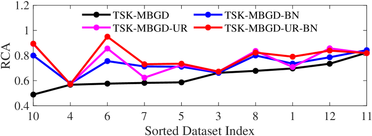
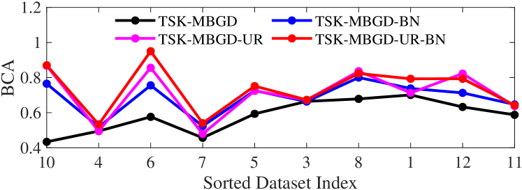
Figure 4: (a) RCAs and (b) BCAs of the four MBGD-based TSK fuzzy classifiers on the 12 datasets. Datasets were sorted according to the RCAs of the TSK-MBGD model. The indices along the horizontal axis denote the dataset indices in Table I.

III-E Statistical Analysis

To further evaluate the performance improvement of our proposed TSK-MBGD-UR-BN over others, we also performed non-parametric multiple comparison tests on the RCAs and BCAs using Dunn’s procedure [41], with a $p$-value correction using the False Discovery Rate method [42]. The results are shown in Table VI, where the statistically significant ones are marked in bold.

Table VI demonstrates that our proposed BN and UR can significantly improve the generalization performance of the traditional MBGD optimization for TSK fuzzy classifiers. TSK-MBGD-UR-BN statistically significantly outperformed CART, JRip, PART, TSK-MBGD and TSK-MBGD-BN on RCA, and also statistically significantly outperformed CART, JRip, TSK-FCM-LSE, TSK-MBGD and TSK-MBGD-BN on BCA. Although the performance improvement of TSK-MBGD-UR-BN over RF and TSK-MBGD-UR were not statistically significant, they were quite close to the threshold, especially for the BCA.

TABLE VI: $p$-values of non-parametric multiple comparisons on the RCAs and BCAs.

	Metric	CART	RF	JRip	PART	TSK-FCM-LSE	TSK-MBGD	TSK-MBGD-BN	TSK-MBGD-UR
TSK-MBGD-BN	RCA	0.0097	0.0628	0.1368	0.3239	0.2723	0.0000	-	-
	BCA	0.1547	0.1627	0.4508	0.0981	0.4518	0.0000	-	-
TSK-MBGD-UR	RCA	0.0001	0.3740	0.0090	0.0460	0.2452	0.0000	0.1146	-
	BCA	0.0036	0.2900	0.0912	0.4420	0.0921	0.0000	0.0731	-
TSK-MBGD-UR-BN	RCA	0.0000	0.2113	0.0002	0.0025	0.0404	0.0000	0.0094	0.1409
	BCA	0.0000	0.0291	0.0021	0.0730	0.0022	0.0000	0.0013	0.0986

III-F Effect of UR

As mentioned in Section II-B, using MBGD to optimize the TSK fuzzy system may face the “rich get richer” problem. To demonstrate this, Fig. 5 shows the average normalized firing levels of the rules on the entire dataset after the four MBGD-based TSK models were trained, on three representative datasets. For TSK-MBGD, a few “richest” rules had much larger average firing levels than others, and hence the rules contributed significantly differently to the output. BN may help alleviate this problem a little bit, as the average normalized rule firing levels in TSK-MBGD-BN were more uniform than those in TSK-MBGD, which also resulted in better classification performances, as demonstrated in the previous subsection. However, UR had the most direct effect on alleviating the “rich get richer” problem, as TSK-MBGD-UR (TSK-MBGD-UR-BN) had much more uniform average normalized rule firing levels than TSK-MBGD (TSK-MBGD-BN), and hence also better classification performance.

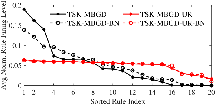
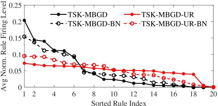
Figure 5: Average normalized rule firing levels of TSK-MBGD, TSK-MBGD-BN, TSK-MBGD-UR and TSK-MBGD-UR-BN on (a) Satellite, (b) Vehicle, and (c) Biodeg datasets.

Note that we set $\tau=1/C$ in (8), where $C=6$ for Satellite, $C=4$ for Vehicle, and $C=2$ for Biodeg. However, the actual average normalized rule firing levels were not exactly $\tau$ on these datasets. Our experiments showed that although UR cannot guarantee the average normalized rule firing levels to be around $\tau$, it can indeed make the rules fired more uniformly.

Why may making the rules fired more uniformly help improve the generalization performance? In [32] we pointed out that a TSK fuzzy system may be functionally equivalent to an adaptive stacking ensemble model, in which each rule can be viewed as a base learner, and the aggregation weights equal the corresponding rule firing levels. When the rule firing levels are more uniform, generally more rules are utilized in computing the output, i.e., more base learners are used in the stacking ensemble model, which may help improve the generalization performance.

To demonstrate this, we computed the entropy of the normalized rule firing levels for each input example:

$$E=-\sum_{r}^{R}\overline{f}_{r}~{}\log\overline{f}_{r},$$ (16)

where $\overline{f}_{r}$ is the normalized firing level of the $r$-th rule. Generally, a larger entropy means more rules were fired.

Fig. 6 shows the histogram of the entropy distributions on the Satellite dataset. When training TSK fuzzy systems without UR, many samples had close to zero $E$, i.e., all except one rule had firing levels close to zero. When UR was added, the number of examples with close to zero $E$ decreased significantly, i.e., more rules with larger firing levels were used in computing the output.

Figure 6: Histogram of the normalized rule firing level entropy $E$ of (a) TSK-MBGD and TSK-MBGD-UR, and, (b) TSK-MBGD-BN and TSK-MBGD-UR-BN, on the Satellite dataset.

III-G Effect of BN

We also used the Satellite dataset to analyze the effect of BN.

We set the UR weight $\lambda=1$ and recorded the training loss and test BCA in the first 20 training epochs. This process was repeated 10 times, and the average results are shown in Figs. 7 and 7, respectively. BN resulted in smaller training losses and better generalization performances in testing.

There is still no agreement on theoretically why BN is helpful in optimizing deep neural networks [24]; thus, it is also challenging to analyze theoretically why BN can help the optimization of TSK fuzzy systems. Nevertheless, we performed an empirical study to peek into this, by recording the L1 norm of the antecedent parameters’ gradients and the L1 norm of the consequent parameters’ gradients in the first 20 training epochs on the Satellite dataset. The results are shown in Figs. 7 and 7, respectively. BN significantly increased the gradients of both antecedent and consequent parameters. With the same learning rate, this can expedite the convergence.

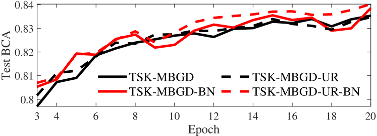
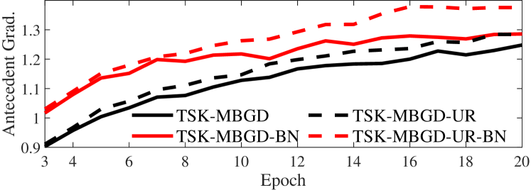
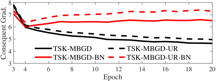
Figure 7: (a) Training loss, (b) test BCA, (c) L1 norm of the antecedent parameters’ gradients, and (d) L1 norm of the consequent parameters’ gradients, in the first 20 training epochs on the Satellite dataset. The horizontal axis starts from 3 epochs so that the differences among the curves can be more clearly visualized.

We also evaluated the performances of the two BN variants introduced in Section II-C. The BCAs of TSK-MBGD-UR, TSK-MBGD-UR-BN, TSK-MBGD-UR-GBN and TSK-MBGD-UR-RBN are shown in Table VII. TSK-MBGD-UR-BN performed the best, and TSK-MBGD-UR-GBN the worst. Since TSK-MBGD-UR-RBN had more parameters to optimize, its training was not as stable as TSK-MBGD-UR-BN and TSK-MBGD-UR-GBN. Therefore, TSK-MBGD-UR-BN is the best choice.

TABLE VII: Average BCAs of the three BN variants on the 12 datasets.

Dataset	TSK-MBGD	TSK-MBGD	TSK-MBGD	TSK-MBGD
	-UR	-UR-BN	-UR-GBN	-UR-RBN
Vehicle	0.7127	0.7930	0.7261	0.7679
Biodeg	0.8390	0.8439	0.8422	0.8440
DRD	0.6717	0.6729	0.6636	0.6650
Yeast	0.4946	0.5332	0.4352	0.5339
Steel	0.7245	0.7515	0.7332	0.7219
IS	0.8559	0.9501	0.9115	0.8938
Abalone	0.4791	0.5402	0.4924	0.5275
Waveform21	0.8362	0.8233	0.8232	0.8334
Page-blocks	0.6033	0.6710	0.5912	0.6333
Satellite	0.8679	0.8700	0.8679	0.8216
Clave	0.6374	0.6421	0.6090	0.6442
MAGIC	0.8225	0.7934	0.8319	0.8318
Average	0.7121	0.7404	0.7106	0.7265

III-H Effect of the Batch Size

The batch size is an important hyper-parameter in MBGD-based optimization. It determines the memory requirement and the convergence speed in training. A larger batch size leads to faster convergence but also requires more memory. In [43], the authors analyzed the effect of the batch size on the generalization performance. Their results showed that using a larger batch size causes degradation in the model generalization performance, because it tends to converge to a shaper minimum, which makes the model sensitive to noise. A similar finding was presented in [44] that a smaller batch size leads to more stable and reliable training. However, since we used the mean, standard deviation and mean firing level of each batch to compute the losses, too small batch size may also lead to poor performance.

We validated our model on the Satellite dataset with batch size varying from 16 to 2,048. The test RCAs and BCAs averaged over 30 runs are shown in Fig. 8. The test performance decreased with too small or too large batch sizes. For TSK-MBGD-UR-BN, it seems that a batch size within [64, 256] is a good choice.

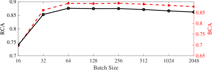
Figure 8: Average RCAs and BCAs of TSK-MBGD-UR-BN on the Satellite dataset, using different batch sizes.

IV Conclusions and Future Research

TSK fuzzy systems are powerful and frequently used machine learning models, for both regression and classification. However, they may not be easily applicable to large and/or high-dimensional datasets. Our very recent research [6] proposed an MBGD-based efficient and effective training algorithm (MBGD-RDA) for TSK fuzzy systems for regression problems. This paper has proposed an MBGD-based algorithm, TSK-MBGD-UR-BN, to train TSK fuzzy systems for classification problems. It can deal with both small and big data with different dimensionalities, and may be the only algorithm that can train a TSK fuzzy classifier on big and high-dimensional datasets. TSK-MBGD-UR-BN integrates two novel techniques, which are also first proposed in this paper:

1. UR, which is a regularization term in the loss function to ensure that all rules are fired similarly on average, and hence to improve the generalization performance.

2. BN, which normalizes the inputs in computing the rule consequents to speedup the convergence and to improve the generalization.

Experiments on 12 UCI datasets from various domains, with varying size and feature dimensionality, demonstrated that each of UR and BN has its own unique advantages, and integrating them can achieve the best classification performance. TSK-MBGD-UR-BN, together with MBGD-RDA proposed in [6], shall greatly promote the applications of TSK fuzzy systems in both classification and regression, especially for big data problems.

The proposed TSK-MBGD-UR-BN also has some limitations, which will be addressed in our future research. First, for very high dimensional data, fuzzy partitions of the input space become very complicated, and numeric underflow may happen when the product $t$-norm is used. Further research shall consider rules that automatically select the most relevant attributes as the antecedents. Second, we shall investigate how to improve the interpretability of data-driven TSK fuzzy systems. This is also partially linked to the first problem, as reducing the number of antecedents can improve the interpretability of the rules.

References

- [1] A.-T. Nguyen, T. Taniguchi, L. Eciolaza, V. Campos, R. Palhares, and M. Sugeno, “Fuzzy control systems: Past, present and future,” IEEE Computational Intelligence Magazine, vol. 14, no. 1, pp. 56–68, 2019.
- [2] Y. Shi, R. Eberhart, and Y. Chen, “Implementation of evolutionary fuzzy systems,” IEEE Trans. on Fuzzy Systems, vol. 7, no. 2, pp. 109–119, 1999.
- [3] D. Wu and W. W. Tan, “Genetic learning and performance evaluation of interval type-2 fuzzy logic controllers,” Engineering Applications of Artificial Intelligence, vol. 19, no. 8, pp. 829–841, 2006.
- [4] L.-X. Wang and J. M. Mendel, “Back-propagation of fuzzy systems as nonlinear dynamic system identifiers,” in Proc. IEEE Int’l Conf. on Fuzzy Systems, San Diego, CA, Sep. 1992, pp. 1409–1418.
- [5] J. S. R. Jang, “ANFIS: Adaptive-network-based fuzzy inference system,” IEEE Trans. on Systems, Man, and Cybernetics, vol. 23, no. 3, pp. 665–685, 1993.
- [6] D. Wu, Y. Yuan, J. Huang, and Y. Tan, “Optimize TSK fuzzy systems for big data regression problems: Mini-batch gradient descent with regularization, DropRule and AdaBound (MBGD-RDA),” IEEE Trans. on Fuzzy Systems, 2020, in press. [Online]. Available: https://arxiv.org/abs/1903.10951
- [7] Y. Jin, “Fuzzy modeling of high-dimensional systems: complexity reduction and interpretability improvement,” IEEE Trans. on Fuzzy Systems, vol. 8, no. 2, pp. 212–221, 2000.
- [8] Y. Deng, Z. Ren, Y. Kong, F. Bao, and Q. Dai, “A hierarchical fused fuzzy deep neural network for data classification,” IEEE Trans. on Fuzzy Systems, vol. 25, no. 4, pp. 1006–1012, 2016.
- [9] F.-L. Chung, Z. Deng, and S. Wang, “From minimum enclosing ball to fast fuzzy inference system training on large datasets,” IEEE Trans. on Fuzzy Systems, vol. 17, no. 1, pp. 173–184, 2008.
- [10] M. Nilashi, O. Bin Ibrahim, N. Ithnin, and N. H. Sarmin, “A multi-criteria collaborative filtering recommender system for the tourism domain using Expectation Maximization (EM) and PCA–ANFIS,” Electronic Commerce Research and Applications, vol. 14, no. 6, pp. 542–562, 2015.
- [11] C. K. Lau, K. Ghosh, M. A. Hussain, and C. R. C. Hassan, “Fault diagnosis of Tennessee Eastman process with multi-scale PCA and ANFIS,” Chemometrics and Intelligent Laboratory Systems, vol. 120, pp. 1–14, 2013.
- [12] Z. Deng, K.-S. Choi, Y. Jiang, J. Wang, and S. Wang, “A survey on soft subspace clustering,” Information Sciences, vol. 348, pp. 84–106, 2016.
- [13] Z. Deng, K.-S. Choi, F.-L. Chung, and S. Wang, “Enhanced soft subspace clustering integrating within-cluster and between-cluster information,” Pattern Recognition, vol. 43, no. 3, pp. 767–781, 2010.
- [14] M. J. Gacto, M. Galende, R. Alcalá, and F. Herrera, “METSK-HDe: A multiobjective evolutionary algorithm to learn accurate TSK-fuzzy systems in high-dimensional and large-scale regression problems,” Information Sciences, vol. 276, pp. 63–79, 2014.
- [15] I. Goodfellow, Y. Bengio, and A. Courville, Deep Learning. Boston, MA: MIT press, 2016.
- [16] S. Ruder, “An overview of gradient descent optimization algorithms,” arXiv preprint arXiv:1609.04747, 2016.
- [17] L. Bottou, “Large-scale machine learning with stochastic gradient descent,” in Proc. Int’l Conf. on Computational Statistics. Paris, France: Springer, Aug. 2010, pp. 177–186.
- [18] I. Sutskever, J. Martens, G. Dahl, and G. Hinton, “On the importance of initialization and momentum in deep learning,” in Proc. Int’l Conf. on Machine Learning, Atlanta, GA, Jun. 2013, pp. 1139–1147.
- [19] D. P. Kingma and J. Ba, “Adam: A method for stochastic optimization,” in Proc. Int’l Conf. on Learning Representations, San Diego, CA, May 2015.
- [20] A. C. Wilson, R. Roelofs, M. Stern, N. Srebro, and B. Recht, “The marginal value of adaptive gradient methods in machine learning,” in Proc. Advances in Neural Information Processing Systems, Long Beach, CA, Dec. 2017, pp. 4148–4158.
- [21] N. S. Keskar and R. Socher, “Improving generalization performance by switching from Adam to SGD,” arXiv preprint arXiv:1712.07628, 2017.
- [22] L. Luo, Y. Xiong, Y. Liu, and X. Sun, “Adaptive gradient methods with dynamic bound of learning rate,” in Proc. Int’l Conf. on Learning Representations, New Orleans, LA, May 2019.
- [23] S. Ioffe and C. Szegedy, “Batch normalization: Accelerating deep network training by reducing internal covariate shift,” in Proc. Int’l Conf. on Machine Learning, Lille, France, Jul. 2015.
- [24] S. Santurkar, D. Tsipras, A. Ilyas, and A. Madry, “How does batch normalization help optimization?” in Proc. Advances in Neural Information Processing Systems, Montréal , Canada, Dec. 2018, pp. 2483–2493.
- [25] J. L. Ba, J. R. Kiros, and G. E. Hinton, “Layer normalization,” arXiv preprint arXiv:1607.06450, 2016.
- [26] L. Fan, “Revisit fuzzy neural network: Demystifying batch normalization and ReLU with generalized hamming network,” in Proc. Advances in Neural Information Processing Systems, Long Beach, CA, Dec. 2017, pp. 1923–1932.
- [27] D.-A. Clevert, T. Unterthiner, and S. Hochreiter, “Fast and accurate deep network learning by exponential linear units (ELUs),” arXiv preprint arXiv:1511.07289, 2015.
- [28] Y. Wu and K. He, “Group normalization,” in Proc. European Conf. on Computer Vision, Munich, Germany, Sep. 2018, pp. 3–19.
- [29] R. A. Jacobs, M. I. Jordan, S. J. Nowlan, and G. E. Hinton, “Adaptive mixtures of local experts,” Neural Computation, vol. 3, no. 1, pp. 79–87, 1991.
- [30] H. Bersini and G. Bontempi, “Now comes the time to defuzzify neuro-fuzzy models,” Fuzzy Sets and Systems, vol. 90, no. 2, pp. 161–169, 1997.
- [31] H. Andersen, A. Lotfi, and L. Westphal, “Comments on ‘functional equivalence between radial basis function networks and fuzzy inference systems’ [and author’s reply],” IEEE Trans. on Neural Networks, vol. 9, no. 6, pp. 1529–1532, 1998.
- [32] D. Wu, C.-T. Lin, J. Huang, and Z. Zeng, “On the functional equivalence of TSK fuzzy systems to neural networks, mixture of experts, CART, and stacking ensemble regression,” IEEE Trans. on Fuzzy Systems, 2020, in press. [Online]. Available: https://arxiv.org/abs/1903.10572
- [33] T. Shen, M. Ott, M. Auli, and M. Ranzato, “Mixture models for diverse machine translation: Tricks of the trade,” arXiv preprint arXiv:1902.07816, 2019.
- [34] N. Shazeer, A. Mirhoseini, K. Maziarz, A. Davis, Q. Le, G. Hinton, and J. Dean, “Outrageously large neural networks: The sparsely-gated mixture-of-experts layer,” arXiv preprint arXiv:1701.06538, 2017.
- [35] K. He, X. Zhang, S. Ren, and J. Sun, “Deep residual learning for image recognition,” in Proc. IEEE Conf. on Computer Vision and Pattern Recognition, Las Vegas, NV, Jun. 2016, pp. 770–778.
- [36] S. Zagoruyko and N. Komodakis, “Wide residual networks,” arXiv preprint arXiv:1605.07146, 2016.
- [37] G. Huang, Z. Liu, L. Van Der Maaten, and K. Q. Weinberger, “Densely connected convolutional networks,” in Proc. IEEE Conf. on Computer Vision and Pattern Recognition, Honolulu, HI, Jul. 2017, pp. 4700–4708.
- [38] E. Frank and I. H. Witten, “Generating accurate rule sets without global optimization,” in Proc. Int’l Conf. on Machine Learning, San Francisco, CA, Jul. 1998.
- [39] W. W. Cohen, “Repeated incremental pruning to produce error reduction,” in Proc. Int’l Conf. on Machine Learning, Tahoe City, CA, Jun. 1995.
- [40] J.-S. R. Jang, C.-T. Sun, and E. Mizutani, “Neuro-fuzzy and soft computing-a computational approach to learning and machine intelligence,” IEEE Trans. on Automatic Control, vol. 42, no. 10, pp. 1482–1484, 1997.
- [41] O. J. Dunn, “Multiple comparisons using rank sums,” Technometrics, vol. 6, no. 3, pp. 241–252, 1964.
- [42] Y. Benjamini and Y. Hochberg, “Controlling the false discovery rate: A practical and powerful approach to multiple testing,” Journal of the Royal Statistical Society: Series B, vol. 57, no. 1, pp. 289–300, 1995.
- [43] N. S. Keskar, D. Mudigere, J. Nocedal, M. Smelyanskiy, and P. T. P. Tang, “On large-batch training for deep learning: Generalization gap and sharp minima,” in Proc. Int’l Conf. on Learning Representations, Toulon, France, Apr. 2017.
- [44] D. Masters and C. Luschi, “Revisiting small batch training for deep neural networks,” arXiv preprint arXiv:1804.07612, 2018.