HISS, a new tool for H i stacking: application to NIBLES spectra
Abstract
H i stacking has proven to be a highly effective tool to statistically analyse average H i properties for samples of galaxies which may or may not be directly detected. With the plethora of H i data expected from the various upcoming H i surveys with the SKA Precursor and Pathfinder telescopes, it will be helpful to standardize the way in which stacking analyses are conducted. In this work we present a new python-based package, HISS, designed to stack H i (emission and absorption) spectra in a consistent and reliable manner. As an example, we use HISS to study the H i content in various galaxy sub-samples from the NIBLES survey of SDSS galaxies which were selected to represent their entire range in total stellar mass without a prior colour selection. This allowed us to compare the galaxy colour to average H i content in both detected and non-detected galaxies. Our sample, with a stellar mass range of , has enabled us to probe the H i-to-stellar mass gas fraction relationship more than half an order of magnitude lower than in previous stacking studies.
keywords:
galaxies: evolution – methods: data analysis – galaxies: ISM1 Introduction
How galaxies evolve over cosmic time is currently a key area of research in astrophysics. A great deal is already known about the evolution of the stellar content of galaxies due to recent infrared (Spitzer, Werner
et al. 2004), optical (Sloan Digital Sky Survey, York et al. 2000), and ultraviolet (Galaxy Evolution Explorer, Bianchi & GALEX
Team 2000) surveys. However, comparatively little is known about the evolution of the gas in galaxies. Understanding how the cold gas evolves is important as it is the raw fuel for the formation of stars and thus galaxies.
Neutral atomic hydrogen (H i) forms the most significant reservoir of neutral gas in galaxies. Studies have shown that blue, star-forming galaxies have a higher fraction of H i gas compared to red, quiescent galaxies (e.g. Roberts &
Haynes, 1994; Gavazzi
et al., 1996; McGaugh &
de Blok, 1997; Cortese et al., 2011; Fabello et al., 2011; Brown et al., 2015), which suggests that H i plays an important role in star formation. H i is difficult to detect in most galaxies beyond the local universe () with existing radio telescopes due to the weak nature of the emission. Researchers have had to exploit different techniques in order to measure very weak H i signals from galaxies. One such technique is H i stacking; with this technique, an average H i mass per galaxy can be estimated by co-adding the H i spectra of a sample of galaxies in which H i is not necessarily directly detected.
The idea of co-adding the undetected H i spectra in studies of the gas content in galaxies was first presented by Zwaan
et al. (2001) and Chengalur
et al. (2001). Both groups were studying the H i within galaxies located in and around clusters. With low detection counts in their samples, both groups independently co-added the non-detections in an effort to obtain a statistically meaningful averaged detection for their samples.
Stacking analyses have become commonplace in the last years. The technique has been applied in various areas: H i content of galaxies in dense environments and how the gas content relates to other observables (Chengalur
et al., 2001; Verheijen et al., 2007; Lah et al., 2009; Jaffé
et al., 2016); gas content of active galaxies (Geréb et al., 2013, 2015); measurement of at low to intermediate () redshifts (Lah et al., 2007; Delhaize et al., 2013; Rhee et al., 2013; Rhee
et al., 2016); and using stacking to study the relations between H i and various stellar mass/star formation indicators (Fabello et al., 2011, 2012; Brown et al., 2015; Brown
et al., 2017; Geréb et al., 2015).
The gas scaling relations for galaxies are average trends which relate the H i mass () or H i mass to stellar mass () ratio (gas fraction, ) to various other galaxy properties. Stacking a sample of 5000 galaxies with that had both ultraviolet and optical imaging, Fabello et al. (2011) found using H i stacking that the gas fraction correlates better with colour than stellar mass. This result was later confirmed and extended to a sample with by Brown et al. (2015). To date, studies of the H i gas scaling relations have been limited to samples with , a mass which has been identified as a turning point around which the vs slope changes (Huang et al., 2012; Maddox et al., 2015).
Directly detecting H i with current radio telescopes beyond is challenging due to the long observing times required (e.g. HIGHz (Catinella &
Cortese, 2015) on Arecibo using and CHILES (Fernández
et al., 2016; Hess et al., 2018) on the JVLA requiring of observing time). The upcoming surveys with the SKA Precursors and Pathfinders (e.g. MeerKAT, Booth
et al. 2009; ASKAP, Johnston
et al. 2008; APERTIF, Verheijen et al. 2008) will greatly extend the redshift range over which H i in galaxies is studied, either directly or indirectly. Techniques such as H i stacking will have an important role to play in order to study the average H i properties of different galaxy samples, particularly at higher redshifts (). Deep SKA Precursor surveys such as LADUMA111Looking At the Distant Universe with the MeerKAT Array (Holwerda
et al., 2011) on MeerKAT have identified stacking as an important tool to probe higher redshifts, and push to lower H i mass limits.
As we rapidly approach the start of the Precursor Surveys, work is under-way on developing a data analysis toolkit that will enable consistent and comparable studies of the survey data. Already available is the versatile source finder, SoFiA (Serra et al., 2015). With the important role that stacking will play in the analysis of high redshift and low mass samples, it is imperative that a tool capable of reliably and consistently stacking H i spectra is developed.
In this work, we present our new software package, HISS, that has been designed for the astronomy community in response to the need for a stacking software package. HISS can be downloaded from https://github.com/healytwin1/HISS. We use HISS to revisit the gas scaling relations with a sample of 1000 galaxies from the Nançay Interstellar Baryon Legacy Extragalactic Survey (NIBLES van Driel
et al., 2016). NIBLES is an SDSS-selected targeted H i survey with the Nançay Radio Telescope which aims to study the H i properties of galaxies as a function stellar mass, covering a representable range of the ensemble of galaxies in the nearby Universe.
The outline for this paper is as follows: the first half of the paper (Section 2) describes the design of the H i Stacking Software (HISS). In the second half of the paper (Section 3 and Section 4), we give an introduction to the NIBLES Survey and the ancillary data we use in our stacking analysis and describe the classification of H i non-detections. We use the NIBLES sample to explore the well-known H i mass to stellar mass scaling relations in Section 4, and finally, summarise our findings in Section 5.
2 The H i Stacking Software (HISS)
The stacking method that the software needs to implement can be summarized by the following steps:
-
1.
Ingest 1D H i spectra (radio data) and list of associated redshifts for the sample of galaxies to be stacked;
-
2.
Spectrally shift and re-scale the H i spectra to align the expected line emission at a common frequency (usually the H i rest frequency: );
-
3.
Weight the spectra (according to a preferred weighting scheme) and co-add the spectra.
We have designed and created the H i Stacking Software (HISS) package, after discussion with colleagues and with the following guiding principles in mind:
-
•
be freely available in most operating systems
-
•
to be open source
-
•
easy to modify (extensible)
-
•
stack hundreds or thousands of galaxy spectra in an efficient and reliable manner.
The Python222Developed in Python 2.7, but compatible with Python 3 programming language was chosen for development of HISS because it is freely available, can be used on any operating system, and is also one of the most commonly used languages within the astronomy community. Where appropriate, HISS makes use of the publicly available Python modules (such as AstroPy, NumPy, SciPy, etc.) which have been optimized for data input, manipulation, and display.
Fig. 1 shows a flow diagram of how the processes required to create a stacked spectrum are incorporated in the different modules of HISS. In the sections that follow we will illustrate how each of the processes highlighted in Fig. 1 are implemented. Basic instructions on how to run HISS can be found in Appendix A.1.
2.1 Simulated Data
When developing new data analysis tools, one of the most important steps is to quantify the accuracy and reliability of any generated results. For this purpose, simulated spectra are used instead of real spectra because properties of the input data are then well known. In this work, we use a data set of 1000 simulated H i profiles of galaxies to illustrate and test the capabilities of HISS. The simulated H i spectra are created using the formulation outlined in Obreschkow et al. (2009c, Appendix A), and are based on the evaluated properties extracted from the -SAX catalogue (Obreschkow et al., 2009a; Obreschkow et al., 2009b, c) for galaxies in a redshift range of with a channel width of and Gaussian noise of per channel.
2.2 Catalogue of H i spectra
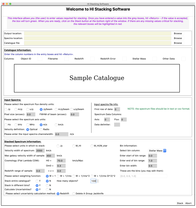
When initiated, HISS requires some information about the sample of H i spectra – see Fig. 2 for an overview. The Input Module requires two input files: a configuration file and a catalogue file. There are two ways to provide HISS with the required information: the user can provide a text file in JSON333JSON stands for JavaScript Object Notation, a JSON formatted file has the extension .json format or use the graphical user interface shown in Fig. 2 to generate a configuration file (also in JSON format). The JSON format is used for the configuration file as it is easy to read/write, and when imported into Python, the information is dumped into an easy - to - access Python dictionary. The configuration file includes options such as different weighting functions for the stacking procedure, and options to bin the stacking sample based on additional data provided in the catalogue file.
The catalogue file is a user-created text file in CSV444comma separated values format that contains at least the following columns,
-
•
Object ID
-
•
Spectrum filename
-
•
Redshift
-
•
Redshift uncertainty
-
•
Other data (optional)
for each spectrum that the user would like to include in the stack. Although the catalogue file may contain any number of columns, the non-optional columns mentioned above are those that are required to run HISS. Additional columns containing numerical information such as stellar mass or optical colour may be used to refine the catalogue into a number of different sub-samples to be stacked separately. This refining is done through the Bin Module (Fig. 1). In this first version of HISS, bins can only be created using one quantity, e.g. stellar mass or colour, and the stacked results are stored for each sub-sample555In the current implementation this process is sequential i.e. each binned sub-sample of spectra is stacked one after the other. This process will be parallelised in future versions..
During the processing of the configuration file, the code checks that the catalogue file and location of the spectra exist. If these checks are passed, HISS will continue.
2.3 Stacking the spectra
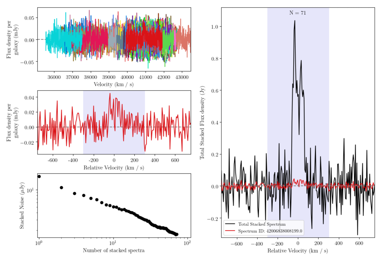
The stacking procedure is the heart of HISS, and is controlled by the Stack Module which is responsible for reading in and preparing each spectrum for stacking, as well as maintaining the stacked spectrum and associated information (e.g.,number of objects in the stack, stacked noise). One of the features of this module is the option that allows the user to watch the progress of the stacking in a window such as the one in Fig. 11. The progress window shows each of the spectra in the observed frame as they are read in, as well as the individual spectra as they are converted to the rest-frame and then added to the total stacked spectrum.
2.3.1 Reading in the spectra
Regardless of how the H i spectra were created, HISS requires that the spectra be in a text file type format containing a column for the spectral axis (either frequency or velocity) and another for the flux density (in units of Jy, mJy, Jy or flux density/beam).
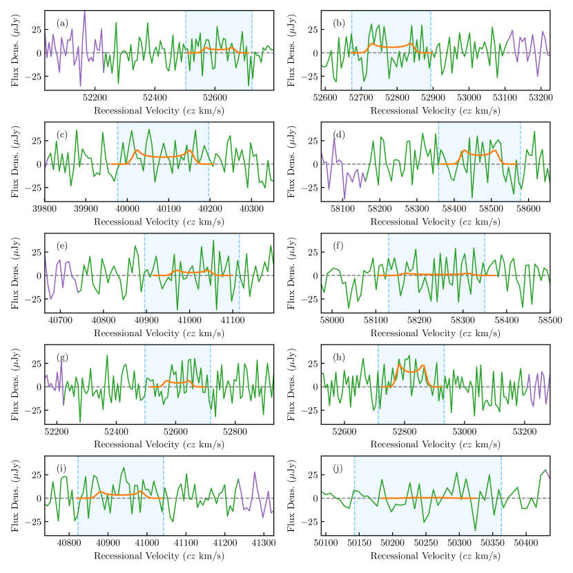
Fig. 12 shows a selection of ten of the 1000 simulated H i profiles that will be used to illustrate the different parts of HISS. Each of these have had Gaussian noise added, so as to simulate the spectra that are anticipated from the deep LADUMA survey.
As each spectrum is read into HISS, it is put through a series of quality checks:
-
•
The spectrum’s channel width is checked to ensure it is within of the entered channel width. A warning is raised if the spectrum channel width is different. If the channel width is more than different the spectrum is discarded.
-
•
The input object contains the minimum and maximum redshift values for the sample of galaxies. This check makes sure that the redshift associated with the spectrum falls within these bounds.
-
•
If the user has decided to stack the spectra in units of gas fraction, the catalogue will be checked for an associated stellar mass value.
-
•
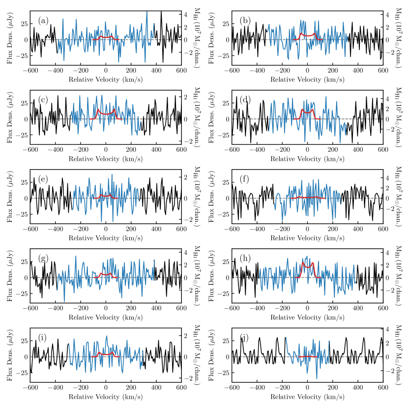
The final check is for spectrum length. A galaxy mask is created based on the expected maximum width galaxy width for the sample. Every spectrum is checked to ensure that it has more channels than the length of mask. An example of a spectrum that would fail such a check is shown in the panel (j) of Fig. 12 and Fig. 13.
Due to the discrete nature of the input spectra, the channel width check is important to avoid co-adding arrays where the rest-frame size of the channel (i.e velocity width in ) changes significantly () between different arrays. The spectra that do not pass at least one of the quality checks are excluded from the stack. The object IDs for the excluded spectra and the reason for exclusion are recorded in the log file.
2.3.2 Convert spectra to rest-frame
If the spectrum passes all the quality checks, it moves to the next step which is to align the spectrum such that the galaxy signal is centred about the central channel of the spectrum. There are two steps to aligning the spectra. The first step is to convert the observed frequencies to a set of rest-frame frequencies corresponding to the systemic velocity of the galaxy being placed at . The spectral axes are converted to the rest frame by
| (1) |
where and are the spectrum’s spectral axis in either velocity or frequency, respectively. The galaxy’s redshift is , and is the speed of light given in kilometres per second.
An input spectrum with a velocity spectral axis is assumed to have rest frame channel widths; this means that the conversion from the observed frame to the rest frame only requires a shift from the recessional velocity to as given by the velocity relation in Eq. 1. For a spectrum with a frequency spectral axis, the rest frame channel width is larger than the observed frame by a factor of ; thus in order to convert the spectrum to the rest frame, both the spectral axis and flux density must be appropriately scaled such that the integrated line flux density is conserved. The frequency axis is converted to the rest frame using the frequency relation in Eq. 1, and the flux is scaled according to: .
2.3.3 Spectrum wrapping
The second step is to shift the galaxy emission to the centre of the spectrum. Since the spectra are now in the rest frame, the target emission is located at either or (depending on the units of the spectral axis) and is easily shifted to the centre of the spectrum. In this step, some authors (e.g., Zwaan
et al., 2001) will concatenate the spectra such that every channel has the same number of measurements (i.e. all of the spectra are the same length). Other authors (e.g., Lah et al., 2007, 2009; Rhee et al., 2013) do not concatenate the spectra, instead choosing to weight each channel in the stacked spectrum relative to the number of measurements in that channel.
Instead, HISS wraps the flux that would be shifted out of the now centred spectrum to append to the other end of the spectrum so that the original spectrum length is maintained; this method also maintains the spectrum noise properties. This is illustrated in Fig. 12: the green part of the spectrum is the main part that is shifted to the centre and purple highlights the section of the spectrum that is appended to the other side of the spectrum array. The centred spectra are shown in blue in Fig. 13. It is clear from each of the panels of input spectra in Fig. 12 that the spectra need not all be the same length. Each spectrum is thus converted to some appropriate length specified by the user as an input parameter, (see bottom block of Fig. 2 – Velocity width of spectrum666The default length is which is width of a galaxy rotating at . A wider spectral axis is not advised due to possible noise variations across the bandwidth.)
In order to avoid issues with small number statistics in the spectrum noise calculations, the length of the stacked spectrum should be at least three times the width of the broadest galaxy profile (i.e., the largest ). The spectra that are longer than necessary are simply truncated at the edges while keeping the galaxy emission at the centre of the spectrum. The shorter spectra are extended by using the so-called “noisy” channels from the outer channels that are not expected to contain any galaxy emission to fill up the new empty channels at either edge of the spectrum.
In order to determine which channels contain only noise, the galaxy emission is masked. The galaxy mask is centred at the spectral location of the galaxy and has some pre-determined width (this is usually a conservative estimate on the maximum possible velocity width of galaxies in the sample). In Fig. 12, for illustrative purposes, the galaxy emission is masked using the pale blue band, all other channels are considered to contain only noise, and so can be used in the spectrum extension process. There are some caveats associated with this process: if there are too few noisy channels in the spectrum, then a ringing phenomenon may appear in the extended spectrum. Fig. 13 shows the original spectra centred in blue, while black indicates the noise that has been used to fill up the channels of the extended spectrum. Fig. 13 (j) highlights the ringing phenomenon.
2.3.4 Co-adding the spectra
Before adding each rest-frame spectrum to the stack, the spectra are converted to the units (Jy, , ) that the user specified as the “stacking units” during the configuration process.
To convert the H i flux density to H i mass, we use the following relation from Wieringa et al. (1992):
| (2) |
where is the galaxy redshift and the associated luminosity distance. is the galaxy rest frame integrated line flux density for the profile in . This relation between the flux density and the H i mass assumes a spherical H i cloud that is optically thin with a uniform internal velocity distribution.
The H i gas fraction (or more accurately, the H i to stellar mass ratio) is simply
| (3) |
where is the total stellar mass and is the total H i mass. The right -axes of the spectra in Fig. 13 are in units of per channel; this choice of units allows us to simply add the values in each channel together when measuring the integrated value.
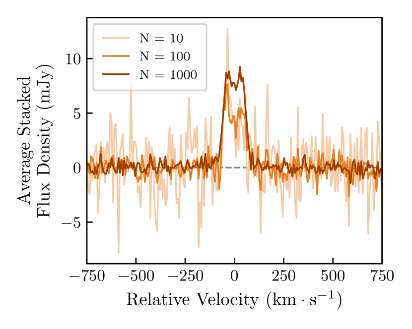
The final step required to produce a stacked spectrum is to co-add the spectra. This is typically done as a weighted average. The benefit of using the average is that Gaussian noise decreases proportional to ( is the number of profiles included in the stacked spectrum), which is favourable to the creation of a spectrum with a higher signal-to-noise ratio, S/N. Fig. 3 shows how the average noise decreases as the number of profiles (in our simulated sample) included in the stack increase. The weighted average is defined by
| (4) |
where is the number of the spectrum to be included in the stack and is the total number of spectra in the sample. Each spectrum has an associated weighting factor . By default, the weighting factor is 1, but the user may choose an alternate option such as
where is the RMS of the channels in a spectrum that contains no galaxy emission (i.e. the noisy channels), and is the luminosity distance to the galaxy. We use the interquartile range of each spectrum as the noise estimate over the conventional standard deviation in order to deal with outlying high or low values for example from RFI spikes.
2.3.5 Reference/Control Spectrum
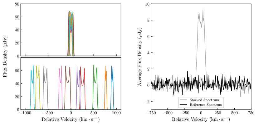
The practice of creating a reference spectrum has been used since the first H i stacking experiments. A reference spectrum is a stacked spectrum created by stacking the spectra in the target sample using the incorrect redshift to align the spectra. The various stacking studies have used two methods to create the reference spectrum. Some authors, who have had access to the radio data cube from which the H i spectra were extracted, choose to create the reference spectrum by extracting spectra from random spatial locations in the data cube and using the target redshifts to align the spectra (e.g., Zwaan
et al., 2001). Other authors use the spectra from their sample but randomize the sample redshifts (e.g., Chengalur
et al., 2001; Delhaize et al., 2013). By randomising the sample redshifts, both the reference spectrum and the stacked spectrum have the same systematics arising from the shifting process (Chengalur
et al., 2001). If the redshifts are randomly assigned to the sample spectra, the resulting average spectrum should take the appearance of a noise spectrum. If this is the case, it provides further confirmation that a detection in a stacked spectrum is legitimate.
The left panels of Fig. 4 show how when the spectra are converted to the rest frame with the wrong redshift they end up completely misaligned. Each of the spectra in the bottom left panel of Fig. 4 has been shifted using the redshift belonging to one of the other galaxies. The result of co-adding the misaligned spectra using Eq. 4 is shown by the black line in the right panel of Fig. 4. The lack of any significant emission at supports the integrity of the detection of the corresponding stacked spectrum that has been created using the correct redshifts. For comparison, the thin grey line shows the stacked spectrum of the correctly aligned spectra.
2.4 Analysing the stacked spectrum
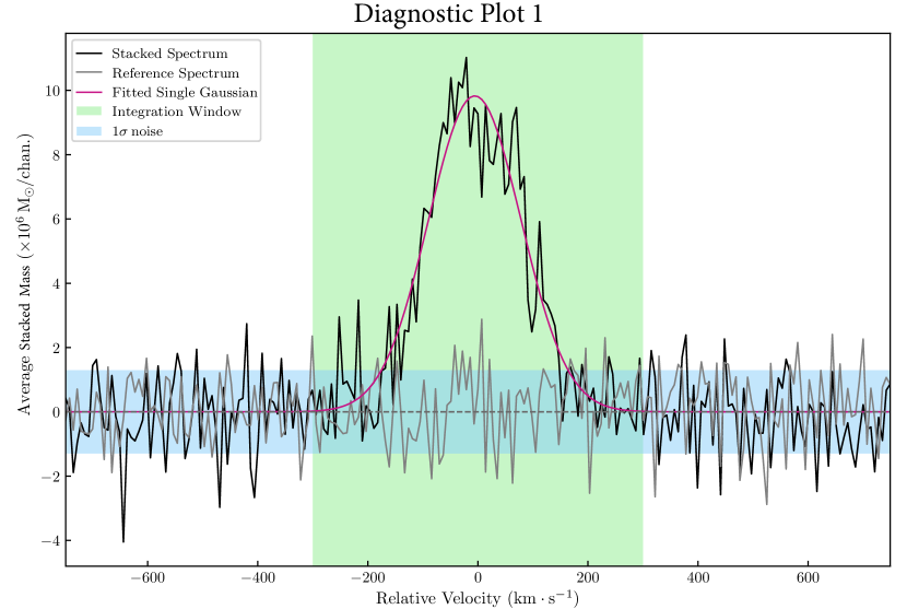
The Analysis Module provides the user with a collection of statistics, spectrum manipulation and profile characterisation routines without the need for third-party software. Upon initialisation of the Analysis Module, an initial statistical analysis is performed and the results are displayed either to a window or to the command line if running in suppress mode. At this point the first visual of the stacked spectrum is displayed in the form of Diagnostic Plot 1 (see Fig. 14.) The user is also asked if the integration window size should be changed from its setting from the input phase777The original integration window is specified by the user when setting Max galaxy velocity width of sample (see bottom block of Fig. 2). The next steps are then displayed to the user:
2.4.1 Profile detection statistics
The collection of statistics that are calculated by this module all characterise the significance of the possible detections in the stacked spectrum in some way. The statistics are displayed in the terminal after calculation, and are saved in the log file for perusal after HISS has completed. The statistical analysis of the stacked spectrum includes three different methods of calculating the signal-to-noise ratio (S/N):
-
•
peak flux density () to noise ():
(5) where is the maximum value of the spectrum within the integration window.
-
•
integrated signal-to-noise:
(6) where is the flux density (in Jy) associated with channel , is the rms noise, dv is the channel width (in ), and is the number of channels integrated over.
-
•
ALFALFA S/N (from Haynes et al., 2011):
(7) where the integrated flux density of the detection is given by (Jy ), () is the width of the spectrum at the peak value888The W50 is obtained from the single Gaussian fit to the spectrum shown in Fig. 14., and is the velocity resolution of the spectrum (this is also called the channel width, unless the spectrum has been smoothed along the spectral axis).
The next statistic calculated is the probability that the signal in a stacked spectrum arises due to a random fluctuation – this is known as the p-value, which will be as low as possible for a strong detection, from which the significance level of the detected signal can be calculated. This is done by fitting a single Gaussian to the spectrum and calculating the value. The single Gaussian is used in favour of other models as it is the simplest model that can describe the shape of an H i detection to first order; please note that in the case of a very clear detection which cannot be characterised by a single Gaussian, the p-value statistic provides no extra information. The null hypothesis is a horizontal line at zero.
2.4.2 Spectrum manipulation
In order to boost the S/N of a stacked spectrum, the Analysis Module offers the user the choice of either re-binning the data (lowering the data resolution, this method has been used by Lah et al., 2007; Rhee
et al., 2016), or smoothing the spectrum using either a boxcar algorithm or a Hanning Window.
All three manipulation routines allow the user to select either the window or the number of old bins to be rebinned into new bins. HISS will not continue to the next step until the user is satisfied with the new version of the stacked spectrum. Diagnostic Plot 2 (which is identical to Diagnostic Plot 1, Fig. 14, but displays the updated spectrum) along with a recalculation of the initial statistics is produced every time a change is made to the spectrum.
2.4.3 Profile characterisation
Given that stacked spectra can have very low S/N, with a lot of noise spikes and dips that are unhelpful in determining the integrated flux density and line width, fitting a function to a stacked spectrum can assist in estimating the stacked profile properties. For example, determining the H i line width () of stacked spectra can be useful for studies such as determining the H i Tully-Fisher relation999An empirical relation which relates the luminosity of galaxy to its rotation velocity (Tully & Fisher, 1977). of non-detected galaxies (Meyer et al., 2016). The analysis module prompts the user to choose from a selection of seven different functions (between one and seven can be chosen simultaneously) that have been used in previous H i studies to characterise H i line profiles:
-
1.
Single Gaussian
-
2.
Double Gaussian
-
3.
Lorentzian Distribution
-
4.
Voigt Profile
-
5.
3rd Order Gauss-Hermite Polynomial
-
6.
Busy Function (Westmeier et al., 2014) – with double-horn
-
7.
Busy Function – without double-horn
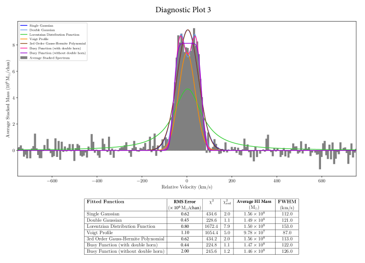
Fig. 15 shows the 7 functions fitted to the stack of the 1000 simulated profiles. Also shown is a table containing the integrated flux density, a measure of the goodness of fit, and the full-with at half-maximum (FWHM) of the fitted function. The user may select any number of the functions, and HISS checks that the user is satisfied with the selection before continuing. A version of Fig. 15 is saved in PNG101010Portable Network Graphics format in the output location as Diagnostic Plot 3. The diagnostic plot is saved to file if HISS is run in suppress mode (an option the user may select when initialising HISS which suppresses all displayed output) so that the user may inspect the function fit before continuing with the analysis.
2.4.4 Uncertainty calculation
The Uncertainty Module allows for two types of uncertainty calculations: a statistical error analysis and a redshift error analysis. The user specifies the type of uncertainty calculation (the two methods cannot be run simultaneously). The Uncertainty Module facilitates the storing of the final analysis options chosen by the user and uses those options to repeat the stacking process 1000 times, each time with slightly different parameters. Fig. 1 indicates the Uncertainty Module as a wrapper around the Stack and Analysis modules.
1. Redshift error analysis: if the user chooses to engage the redshift uncertainty calculations, another loop is activated around the Stack and Analysis Modules which repeats the two processes one thousand times. In every iteration, the redshift associated with each spectrum in the input catalogue is changed by an amount that is selected from a normal distribution with a standard deviation equivalent to the particular spectrum’s redshift uncertainty. Thus, the redshift for each spectrum becomes , where d has been sampled from a normal distribution defined by .
The result of repeating the stack and analysis process means that there are 1000 slightly different versions of the stacked spectrum and their corresponding integrated flux values. Each of the 1000 versions of the analysis object (which each contain a selection of integrated fluxes and the stacked spectrum data) are stored by the Uncertainty Class. Upon completion, the Uncertainty Class processes the stored data: the error bars on the spectrum data are calculated from the minimum and maximum values per channel of the 1000 stored spectra, the data points are given by the mean values. The error-bars on the integrated fluxes are determined from the difference between the mean value (which serves as the quoted value) and the and percentile.
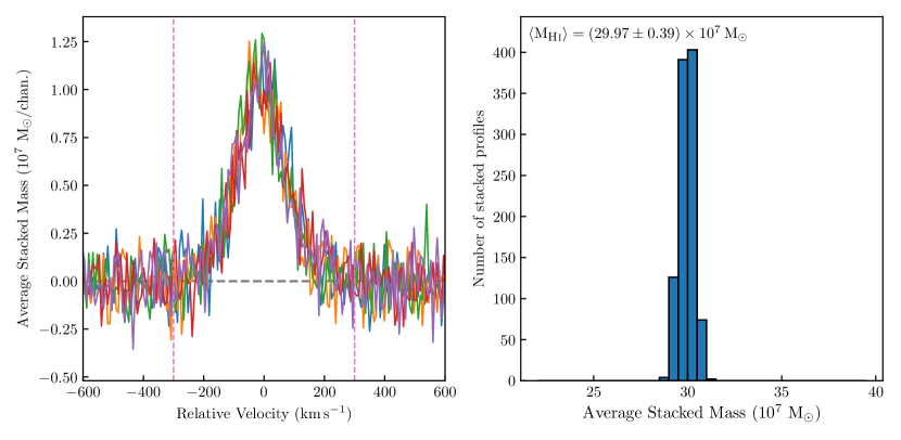
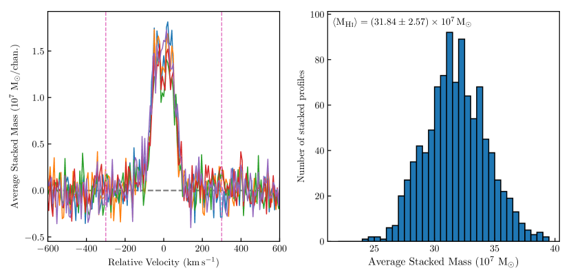
An example of the stacked spectrum using this error calculation method and an average is shown in 5(a).
2. Statistical error analysis: the statistical error analysis implemented by this module is the Delete-A-Group Jackknife (Kott, 2001) error method. In the same way as mentioned above, another loop is activated around the Stack and Analysis Modules repeating the process a thousand times, however each iteration discards a percentage (as chosen by the user) of the total catalogue without replacement. The 1000 analysed stacked spectra are stored by the Uncertainty Module. The flux values for the final stacked spectrum are taken as the mean value of the 1000 versions in each channel. The error bars on the flux in each channel are calculated according to
| (8) |
where is the number of repeated estimates (which would be 4 if only of the population was used for each iteration), is the flux for the particular channel of the nth subset, and is the mean flux value for the particular channel (Kott, 2001; Brown et al., 2015). This is illustrated in 5(b).
The shape of the redshift error analysis profile is smeared out into a more Gaussian shape than the statistical error analysis stacked profile due to each spectrum being allocated its correct redshift plus an offset value. This results in the individual line centres being smeared around the zero point. This was also observed by Maddox
et al. (2013).
The choice of preferred error analysis method is left to the user to decide based on their particular sample selection and optical catalogue redshift precision.
2.5 Save Results
There are nine possible files that can be saved to the output location – 5 data files and 4 possible diagnostic plots (these inform user interactions at point 2):
-
1.
Stacked Catalogue: this text file contains a list of all the spectra included in the stack. Along with the data provided by the user from the input catalogue, this table also contains the integrated flux density for each spectrum.
-
2.
Output Data: a FITS table file containing the spectrum data (stacked spectrum, spectral axis and reference spectrum), the fitted parameters of any fitted functions, the stacked noise, and if the spectrum has been smoothed then the original version of the spectrum data is also saved.
-
3.
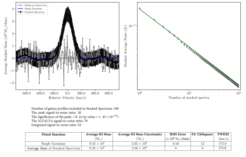
Stacked Spectrum Plot: a PDF file of the stacked spectrum plotted with the fitted functions and the reference spectrum (a version of this is shown in the top left panel of Fig. 17).
-
4.
Stacked Noise Plot: a PDF file of the stacked noise which has the expected line over-plotted (top right panel of Fig. 17).
-
5.
Integrated Flux Data File: a table of the calculated integrated flux from the different functions as well as the flux integrated within the galaxy window. This file is saved in Encapsulated Comma Separated Value (ecsv) format using the AstroPy ASCII module, which allows the units of the flux to be saved to file. Other columns in this file include the goodness of fit values from the function fits. A version of this table is shown in the bottom panel of Fig. 17.
-
6.
Diagnostic Plot 1: this is the first plot of the stacked spectrum that is displayed and saved upon initialisation of the Analysis Module. (Fig. 14)
-
7.
Diagnostic Plot 2: a PNG file that is only produced if the user decides to rebin or smooth the spectrum. This plot is almost identical to Fig. 14.
-
8.
Diagnostic Plot 3: a PNG file that is created when the user selects a function to fit to the stacked spectrum (Fig. 15).
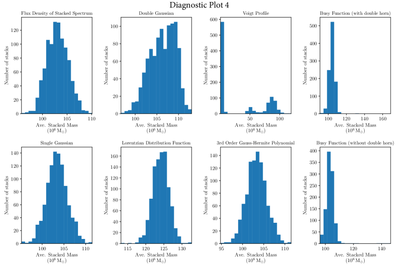
-
9.
Diagnostic Plot 4: this plot is only produced if the uncertainties have been calculated. The plot contains a series of histograms showing the spread of the integrated fluxes. Diagnostic Plot 4 is saved to file in PNG format (Fig. 16).
2.6 Displaying the results
Upon conclusion of the analysis of the stacked spectrum, all calculated quantities and plots are saved to the user-chosen output location. Amongst the saved files is a plot of the stacked spectrum which makes this final module an optional one. The Display module reads in the files saved to disk at the end of the analysis. The results are then displayed in an easy to read manner – the stacked spectrum (along with the reference spectrum) is shown on the top left, to the right of the stacked spectrum is the stacked noise as a function the number of profiles. Below the two plots are the statistics associated with stacked spectrum, and a table containing the calculated integrated fluxes. A screenshot of the display window is shown in Fig. 17.
3 Application of HISS to the NIBLES Survey
In this second half of the paper, we will demonstrate some of the capabilities of HISS by stacking different sub-samples of galaxies observed as part of the Nançay Interstellar Baryon Legacy Extragalactic Survey (NIBLES; van Driel
et al., 2016), and re-visiting the well-known H i scaling relations (e.g. Catinella
et al., 2010, 2012, 2013; Brown et al., 2015).
NIBLES is a targeted H i survey of galaxies selected by , a proxy for stellar mass, from the Sloan Digital Sky Survey (SDSS; York et al., 2000). The H i data were obtained using the Nançay Radio Telescope (NRT) in the centre of France. NIBLES provides a unique opportunity to study the baryonic content in galaxies with a wide range of stellar mass ().
3.1 H i Data
The NIBLES sample of 2600 galaxies was selected from SDSS Data Release 5 (DR5; Adelman-McCarthy et al., 2007). The selected galaxies were chosen to uniformly sample the stellar mass range of the ensemble of galaxies in the local Universe. The particular selection criteria (van Driel et al., 2016) were as follows:
-
1.
The target must have both SDSS DR5 spectroscopy and photometry.
-
2.
NIBLES targets were limited to the Local Volume: .
-
3.
In order to study the H i in galaxies as a function of stellar mass, 150 galaxies were selected per bin for (), if available. was used as a proxy for stellar mass111111SDSS stellar mass catalogues were not yet publicly available at the time of the original NIBLES sample selection which was based on DR5 photometry.;
-
4.
In order to maintain a morphologically diverse sample, no colour selection was made.
In addition to these criteria, van Driel
et al. (2016), when selecting the target galaxies tried to avoid objects in and around the Virgo cluster as well as the ALFALFA .40 footprint (Haynes
et al., 2011). The dense environment in the Virgo cluster is known to have noticeable effects on the H i properties of the galaxies in the region. The distances to galaxies in the Virgo region also have large uncertainties.
The Nançay Radio Telescope (see van Driel
et al. for further details) is a single dish radio telescope located in France. The telescope is a transit instrument with a collecting area of and consists of two large reflectors. At , the NRT beam spans in right ascension and varies in declination from depending on the declination of the source; the exact declination size of the beam can be determined using Eq. 9.
The spectra were collected from January 2007 to December 2010, for a total of 3500 hours of telescope time. Each target was initially observed for roughly using successive ON source and OFF source pointings, which was repeated as required and as observing time permitted. The OFF source pointing was chosen to be of each target. The data reduction process is discussed in detail by van Driel et al. (2016). Each published spectrum has a velocity resolution of and a typical noise level of .
3.1.1 Higher-sensitivity Arecibo follow-up H i observations
An indication that stacking Nançay H i spectra may lead to the detection of a significant signal can be found in the higher sensitivity follow-up observations that were obtained with the 305m Arecibo radio telescope, which resulted in a high detection rate of NRT non-detections (Butcher et al., 2016). Of the Nançay targets, 71 non-detections and 19 marginal detections were observed at Arecibo with a four times higher sensitivity (mean rms ). This led to the detection of 85% and 89% of the NRT non-detections and marginal detections, respectively. It should be noted that most (59, or 66%) of the re-observed NRT non-detections are blue, low mass galaxies () which are expected to be relatively gas-rich (see § 4). Within the same stellar mass range, the of the new Arecibo detections is on average three times lower than for the Nançay detections. Alternatively, using the HISS approach to reach the four times lower Arecibo rms level we could also have stacked 16 NRT spectra. The analysis of similar Arecibo data of a much larger sample of NIBLES Nançay non-detections of all colours has recently been published by Butcher et al. (2018). The Arecibo data mentioned above were not used for the stacking study presented here.
3.1.2 Comparison between NIBLES and other H i surveys
Upon comparison with other single-dish H i surveys (e.g. ALFALFA, HIPASS (Barnes et al., 2001); see Table A.4 in van Driel et al. 2016), the ALFALFA fluxes were found to be higher than the NIBLES fluxes by a factor /NRT . The comparisons between NRT fluxes and the ALFALFA fluxes, as well as possible reasons for the difference in flux scales are discussed in detail in § 4.6 in van Driel et al. (2016). In this work, the NIBLES fluxes are quoted. In the event of comparison between NIBLES measurements and ALFALFA measurements, the ALFALFA measurements are scaled to the NIBLES flux values using the ALFALFA/NRT flux ratio mentioned above.
3.2 Optical Data
The optical photometric data used in this work is obtained from the SDSS Data Release 12 where the photometric quality flag was marked clean with no deblended “child” objects. In the DR12 database, the spectroscopic sources (from which the NIBLES sample is derived) are matched to the “value-added” JHU/MPA catalogues (Brinchmann et al., 2004) which contain the stellar masses used in this work. The catalogue provides a number of different measures of the stellar mass, however for the purposes of the NIBLES analyses, the median values are used (Butcher et al., 2018; van Driel et al., 2016).
3.3 NIBLES Stacking Sample
3.3.1 Accounting for known contamination sources
Studies have shown that galaxies which are nearby to the target galaxies in terms of both distance on the sky and systemic velocity can significantly contribute to the total emission in a target H i galaxy spectrum (Jones et al., 2016; Elson et al., 2016). For example, Elson et al. (2016) showed that for a stacking experiment using simulated Parkes data at resolution at , the average contaminant H i mass per galaxy spectrum was . Thus, before finalising the sample of spectra for stacking, it is necessary to remove spectra that are known to have nearby galaxies that could contribute significant contaminating emission to the spectrum. In other works (e.g., Fabello et al., 2012), a secondary source (irrespective of morphology) is considered to contaminate the target spectrum if it lies spatially within the half-power beam width and of the target. In this work, galaxies near the target source are considered as possible contaminators if
-
•
the secondary galaxy is located spatially within N-S half-power beam width and E-W half-power beam width, and
-
•
the redshift of the secondary galaxy is within of the target redshift.
The above criteria were used to search for sources in both the SDSS Spectroscopic Database and the NASA/IPAC Extragalactic Database (NED). A total of 761 spectra were classified as potentially contaminated using these criteria. For more details see Appendix B.
3.3.2 Defining H i detections vs. non-detections
NIBLES galaxies were originally classified as ‘detected’, ‘marginal’ or ‘not detected’ as explained in van Driel
et al. (2016) by three independent adjudicators, who used statistical parameters describing the profile S/N and also inspected all spectra by eye. For this work we wanted a binary classification of ‘detected’ or ‘not detected’ for our stacking experiments and we wanted to use a method which did not rely on human intervention. Various methods exist for finding signals and classifying detections in H i spectra (see for example Saintonge 2007; Verheijen et al. 2007; Haynes
et al. 2011; Ramatsoku
et al. 2016). Using the original classifications in van Driel
et al. (2016) as a guide, we used classification criteria, adapted from Ramatsoku
et al. (2016) to reproduce the sample selection of van Driel
et al. (2016), while at the same time self-consistently and objectively classifying the marginal detections as either detections or non-detections. This method produced very similar detection classifications to van Driel
et al. (2016) with over overlap in the classifications between the two schemes for both detections and non-detections, and resulted in the NIBLES marginal detections (52) being allocated as detections vs. non-detections in a ratio of one-third to two-thirds in our sample.
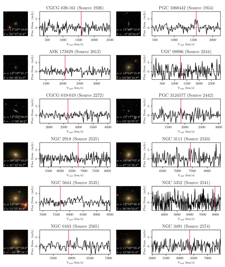
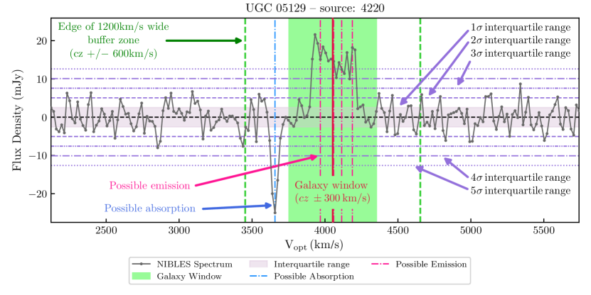
Following Ramatsoku et al. (2016) we classify galaxies as detected if there are a number of consecutive channels above a threshold value. The threshold values are set based on the noise level of the individual spectra which we estimate using the sub-interquartile range (IQR – half the difference between the and flux percentiles). The IQR is less sensitive to outliers in a distribution than the standard deviation and therefore eliminates the need for manual masking of the target source and/or artefacts in the spectrum when estimating the noise (see Fig. 19). For classification of NIBLES spectra, we considered a window of centred on the target redshift. If any emission, satisfying the criteria below, was found in the window, the spectrum was classified as a detection:
-
•
1 or more channels with flux density above IQR (within a window)
-
•
2 or more consecutive channels above IQR
-
•
4 or more consecutive channels above IQR
-
•
5 or more consecutive channels above IQR.
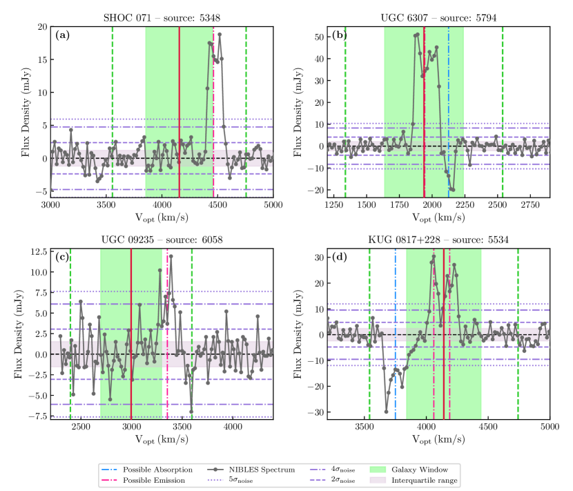
Visually inspecting the spectra after classification showed that some sources had an H i detection in the off-source pointing which presents in the NIBLES spectra as an absorption-like feature, while other spectra had clear emission features from sources not previously identified in our possible contaminant source search (see § 3.3.1.) Examples of spectra with these features are presented in Fig. 20. These features can bias the stacked spectrum and therefore in order to flag these spectra and eliminate them from our sample, we ran the classification algorithm a second time over a wider velocity range ( centred on the target redshift and indicated by the vertical green dashed lines in Fig. 20), to identify possible positive and negative emission not related to the target galaxy. We rejected galaxy spectra that had either negative emission satisfying our classification criteria in any part of the larger search window () or positive emission satisfying the criteria and falling outside a central range of but within . In total 24 spectra were removed from the stacking sample in this way.
3.3.3 Final stacking sample
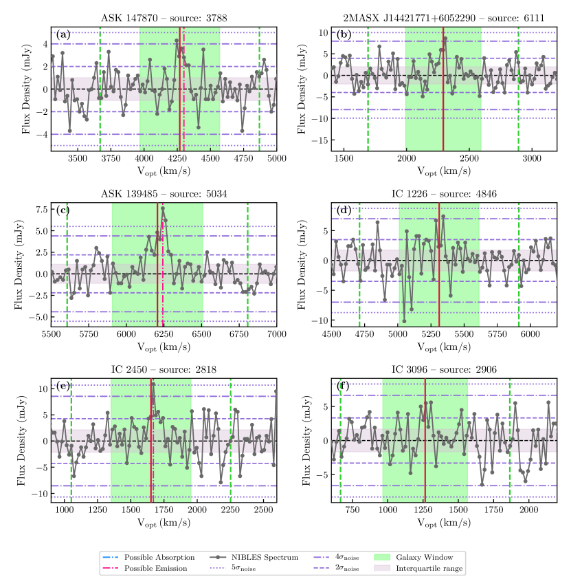
We excluded from our sample galaxies with due to unreliable SDSS photometry and therefore unreliable stellar masses. Our final catalogue consists of 1000 H i spectra deemed free of nearby contaminant emission. Of the 1000 sources, 323 were classified as non-detections and 677 as detections (see Fig. 21 for examples). The catalogue for the non-detections can be found in Appendix E.
4 Gas scaling relations in NIBLES
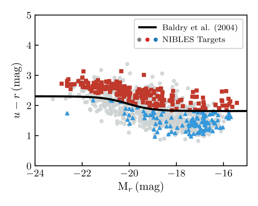
As has been previously stated, the NIBLES sample is morphologically diverse, and it ranges from gas-rich late-type galaxies to gas-poor early-type galaxies. In order to explore the contributions from the different morphological types to the stacked profiles, we separate the stacking sample into red and blue sub-samples using the Baldry et al. (2004, Eq. 9) optimal colour divider as shown in Fig. 6.
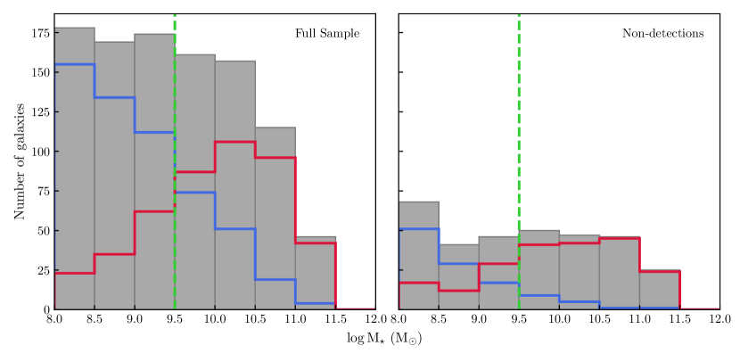
Having separated the full sample into blue and red sub-samples, there are 549 blue galaxies (436 detections, and 113 non-detections) and 451 red galaxies (241 detections, and 210 non-detections). The stellar mass distributions for the full sample and non-detections alone, and each broken down by colour, are shown in Fig. 7.
It is clear in both the full sample and the non-detected sample that the blue galaxies are predominantly in the low- regime, while the red sample contains mainly high- galaxies. The transition from predominantly blue galaxies to predominantly red galaxies occurs in our full sample around which also corresponds to the so-called “gas-richness” threshold (Kannappan et al., 2013) which signifies the transition from H i gas-rich galaxies (at lower ) to H i gas-poor galaxies (at higher ).
4.1 The average H i properties
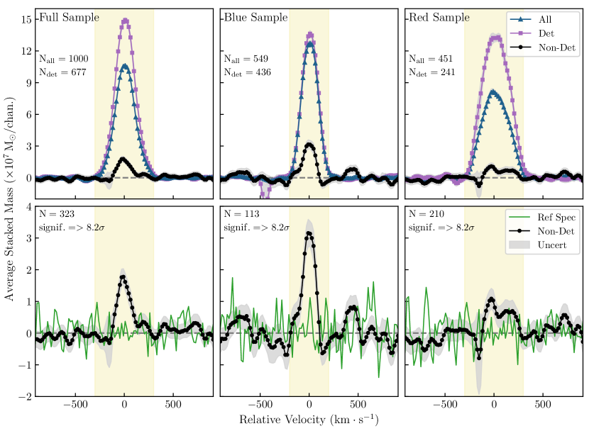
We separated the full sample into three samples: all spectra (full sample), detections only, and non-detections only. The spectra are stacked in units of and the resulting spectra are shown in the left column of Fig. 8. The top row of Fig. 8 shows the stacked profiles for the full sample, detections, and non-detections on the same set of axes; the bottom row shows only the stacked profiles for the non-detections, enlarged for clarity. The top left panel shows the comparison between the stacked spectra for the full sample (blue triangles), and the spectra for the sample of only detections (purple squares) and only non-detections (black filled circles).
The middle and right panels of Fig. 8 show the stacked spectra for the blue and red sub-samples respectively. As indicated by the vertical yellow bands, we integrate over a narrower velocity range for the blue sub-samples compared to the red sub-samples. The blue stacked spectra are expected to be narrower since the average stellar mass of the blue sample is lower than the red sample.
The average H i mass and to ratio () measured from the stacked profiles for each of the nine sub-samples (all galaxies, all blue galaxies, all red galaxies; all H i detections, blue H i detections, red H i detections; all non-detections, blue non-detections, and red non-detections) are shown in Table 3.
H i stacking is a powerful tool to probe the average H i properties of various galaxy samples, however one should have a clear idea of the morphological properties of the galaxies that make up the sample. We have shown how the stacked H i profiles can change by only looking at blue or red galaxies – we find that the stacked profiles for the red samples are wider than the stacked profiles for the blue samples. This is to be expected based on the bimodal distribution of local galaxies where the red galaxies on average have higher stellar masses, and in line with the Tully-Fisher relation, higher rotation velocities (see also Fabello et al., 2011; Meyer et al., 2016).
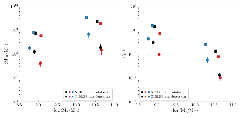
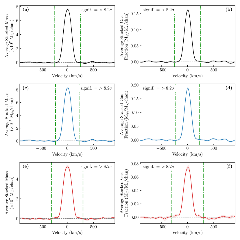
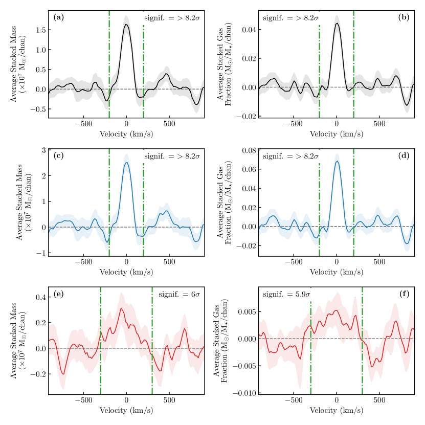
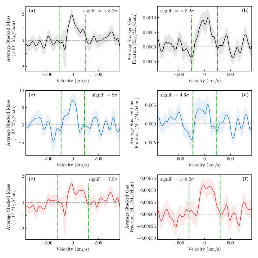
We divided our sample into two bins of low and high stellar mass ( and ) to explore the average H i properties of blue and red galaxies in these 2 samples. As outlined earlier in this paper, HISS is capable of directly determining the average H i mass or H i gas fraction from stacked spectra. The H i-to-stellar mass fraction (gas fraction or ) is a useful tool to probe how gas rich a galaxy or sample of galaxies is. Our results are summarized in Fig. 9 and the stacked profiles are shown in Appendix D.2, with the measured quantities presented in Table 4 and Table 5. Note that all the stacked profiles have S/N and are also classified as detections according to the criteria in § 3.3.2.
These results are consistent with work by Kannappan (2004) which shows that while low mass galaxies tend to have lower H i masses than their high mass counterparts, the low stellar mass galaxies tend to have higher H i gas fractions. The right panel of Fig. 9 highlights what was found by Brown et al. (2015) that the steep slope of the average vs trend (indicated by the black squares and filled circles) from low to high stellar mass is driven by the predominance of high gas fraction blue galaxies at low stellar mass and the low gas fraction red galaxies at high stellar mass. This trend is seen for both the full stacked sample and when stacking non-detections alone.
4.2 Gas fractions in NIBLES galaxies
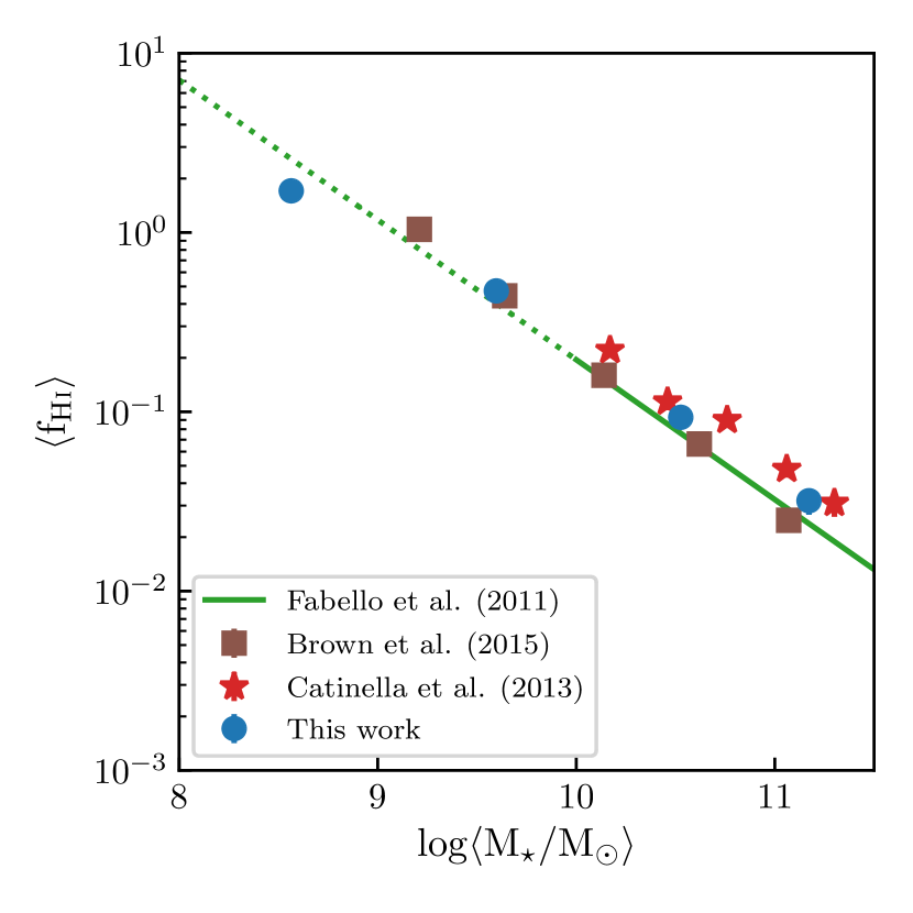
Gas scaling relations have been used in conjunction with stacking (e.g., Fabello et al. 2011, hereafter F11; Brown et al. 2015, hereafter B15) to study various galaxy properties (star formation, stellar mass, etc.) and their influence on the H i content of the galaxies. In Fig. 10 we compare NIBLES gas fractions calculated using HISS to gas fractions from Catinella
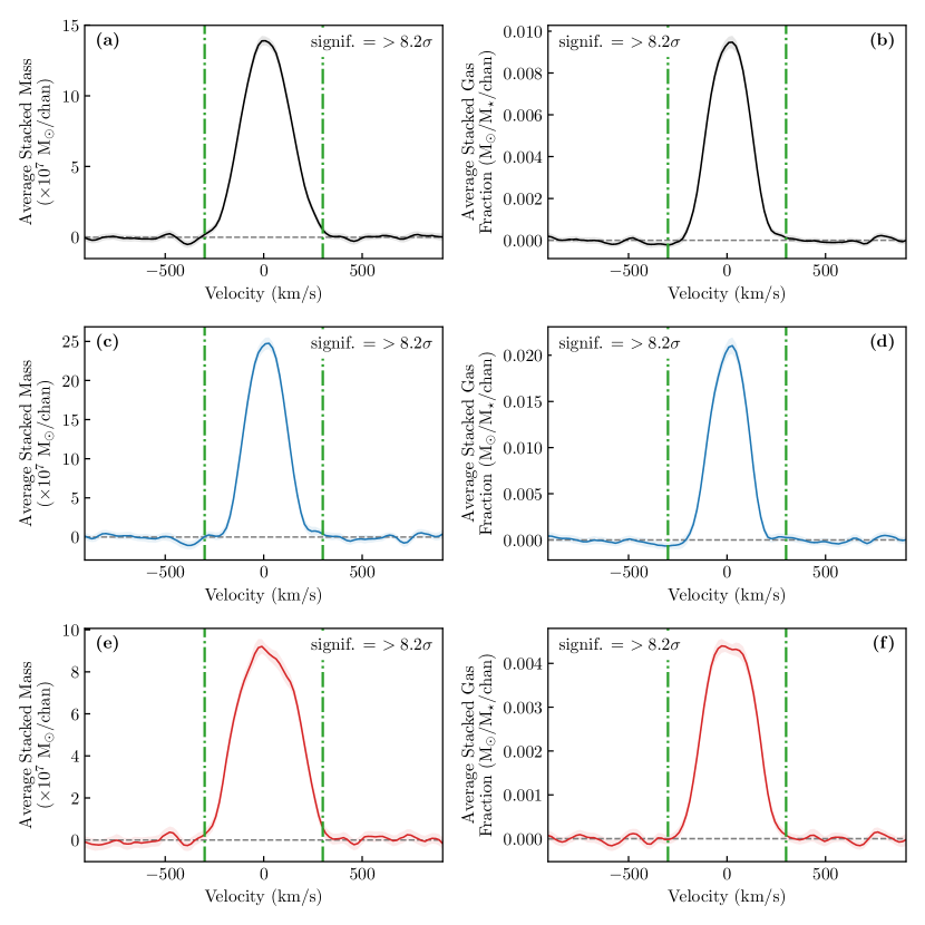
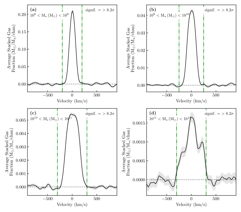
et al. (2013, hereafter C13), F11 and B15. Adopting the method used by B15, we separated the full NIBLES sample (detections plus non-detections) into bins of with widths of . The sample stellar mass distribution is presented in Fig. 7. For the NIBLES sample in Fig. 10 (indicated by the round blue circles), the values represent the mean value in each bin. The NIBLES stacked profiles are presented in Fig. 26 and the measured quantities are listed in Table 1.
The C13 sample was selected from the GALEX Arecibo SDSS Survey (GASS, Catinella
et al., 2010, 2013), a survey with the Arecibo telescope which targeted 1000 massive galaxies randomly selected from the overlap between the SDSS DR6 spectroscopic survey and GALEX Medium Imaging Survey. The F11 and B15 samples are selected from the overlap between ALFALFA, SDSS and GALEX. The C13 results show weighted average values (the H i non-detections are set to upper limits) while the F11 and B15 results are obtained from H i stacking. To take into account the known flux offset between ALFALFA H i spectra and NIBLES (see § 3.1.2), the B15 and F11 gas fractions have been scaled by the mean /NRT flux ratio (). The solid green line is the fit from F11 to their gas scaling relation and the dotted green line represents a linear extrapolation of this trend to lower stellar mass.
Due to the NIBLES sample selection, we are able to go down an order of magnitude lower in stellar mass than previous results by B15. For the NIBLES gas fractions agree well with the results by C13 and the adjusted gas fractions from B15 and F11. Below , the NIBLES is lower than the trend set by the higher stellar mass galaxies.
Huang et al. (2012) and Maddox et al. (2015) have previously noted the change in slope of the vs relation between in the H i-selected population of ALFALFA galaxies where the relation is steeper at lower mass and flatter towards the high mass end. A change in slope is also seen in the ALFALFA - scaling relation by Huang et al. (2012) around a similar where the slope is flatter at lower and drops more steeply at higher . Huang et al. (2012) note that their average gas fraction relation has an overall offset to higher values as expected compared to the optically selected samples by Catinella
et al. (2010) and Cortese et al. (2011) due to the ALFALFA sample bias towards more gas rich galaxies per stellar mass bin. Across the mass range investigated, per bin in stellar mass, they also observe a sharp cut-off in number density at the higher end of the gas fraction distribution, but a large dispersion towards lower gas fractions and note that for surveys with longer integration times, a lower average per stellar mass bin would be observed. A similar change in slope towards lower would also therefore be expected for stellar mass selected samples as for the ALFALFA sample. The divergence of the lowest stellar mass NIBLES gas fraction data point from the higher stellar mass trends from the extrapolated F11 fit is therefore consistent with expectations based on the H i-selected ALFALFA sample Huang et al. (2012) gas fraction vs relation.
| N | Significance | S/N | ||
| 8.56 | 347 (109) | 174.7 | ||
| 9.60 | 335 (96) | 231.8 | ||
| 10.53 | 272 (93) | 216.6 | ||
| 11.17 | 46 (25) | 49.3 |
5 Summary
This work has detailed the development of a new H i spectral stacking package in Python (H i Stacking Software: HISS); while we have exclusively used H i emission spectra to test HISS, it is capable of stacking emission or absorption spectra of any characteristic line. HISS takes the spectra for a sample of galaxies along with the accompanying redshifts recorded in the galaxy catalogue to produce an average spectrum from which a number of average properties (e.g., H i mass , H i-to-stellar mass ratio ) for the sample may be extracted. HISS also offers the user a choice of two built-in error analysis methods, and the ability to characterise the shape of the stacked spectrum through fitting a variety of functions.
We have applied HISS to stacking of 1000 H i spectra from the Nançay Interstellar Baryon Legacy Extragalactic Survey (NIBLES), which is a stellar mass-selected (with no colour-selection) H i survey of SDSS galaxies in the nearby Universe. Due to the wide stellar mass range spanned by the NIBLES dataset (), extending an order of magnitude lower than Brown et al. (2015), we were able to extend the previously studied gas fraction vs. stellar mass gas scaling relation (Brown et al., 2015; Fabello et al., 2011; Catinella et al., 2013) down to lower average stellar mass (). With our stellar mass selected sample, we find good agreement with previous results at high stellar mass. At low stellar mass () we observe a deviation from the extrapolated high mass relation which indicates a flattening of the slope in the scaling relation at low stellar mass qualitatively consistent with the trend seen in the H i-blind, gas-rich ALFALFA sample (Huang et al., 2012).
Acknowledgements
JH acknowledges the bursary provided by South African Radio Astronomy Observatory; SLB, EE, and JH were supported by the South African National Research Foundation. We thank Barbara Catinella and Kelley Hess for their input and advice on the design of HISS. JH wishes to thank S. Makhathini and L. Lindroos for helpful conversations during a trip to OSO, supported by MIDPREP. The Nançay Radio Astronomy Facility is operated as part of the Paris Observatory, in association with the Centre National de la Recherche Scientifique (CNRS) and partially supported by the Région Centre in France. This research has made use of the NASA/IPAC Database (NED) which is operated by the Jet Propulsion Laboratory, California Institute of Technology, under contract with the Nation Aeronautics and Space Administration, and data from Sloan Digital Sky Survey (SDSS-III). Funding for SDSS-III has been provided by the Alfred P. Sloan Foundation, the Participating Institutions, the National Science Foundation, and the U.S. Department of Energy Office of Science. The SDSS-III web site is http://www.sdss3.org/. SDSS-III is managed by the Astrophysical Research Consortium for the Participating Institutions of the SDSS-III Collaboration.
References
- Adelman-McCarthy et al. (2007) Adelman-McCarthy J. K., et al., 2007, The Astrophysical Journal Supplement Series, 172, 634
- Baldry et al. (2004) Baldry I. K., Glazebrook K., Brinkmann J., Ivezić Z., Lupton R. H., Nichol R. C., Szalay A. S., 2004, The Astrophysical Journal, 600, 681
- Barnes et al. (2001) Barnes D. G., et al., 2001, Monthly Notices of the Royal Astronomical Society, 322, 486
- Bianchi & GALEX Team (2000) Bianchi L., GALEX Team 2000, Memorie della Società Astronomia Italiana, Vol. 71, p.1117, 71, 1117
- Booth et al. (2009) Booth R. S., de Blok W. J. G., Jonas J. L., Fanaroff B., 2009, ArXiv eprints, p. 2935
- Brinchmann et al. (2004) Brinchmann J., Charlot S., Heckman T. M., Kauffmann G., Tremonti C., White S. D. M., 2004, ArXiv eprints, astro-ph/0
- Brown et al. (2015) Brown T., Catinella B., Cortese L., Kilborn V., Haynes M. P., Giovanelli R., 2015, Monthly Notices of the Royal Astronomical Society, 452, 2479
- Brown et al. (2017) Brown T., et al., 2017, Monthly Notices of the Royal Astronomical Society, 466, 1275
- Butcher et al. (2016) Butcher Z., Schneider S., van Driel W., Lehnert M. D., Minchin R., 2016, Astronomy & Astrophysics, 596, 20
- Butcher et al. (2018) Butcher Z., Schneider S., van Driel W., Lehnert M. D., 2018, Astronomy & Astrophysics, 619, 14
- Catinella & Cortese (2015) Catinella B., Cortese L., 2015, Monthly Notices of the Royal Astronomical Society, 446, 3526
- Catinella et al. (2010) Catinella B., et al., 2010, Monthly Notices of the Royal Astronomical Society, 403, 683
- Catinella et al. (2012) Catinella B., et al., 2012, Astronomy & Astrophysics, 544, 30
- Catinella et al. (2013) Catinella B., et al., 2013, Monthly Notices of the Royal Astronomical Society, 436, 34
- Chengalur et al. (2001) Chengalur J. N., Braun R., Wieringa M., 2001, Astronomy and Astrophysics, 372, 768
- Cortese et al. (2011) Cortese L., Catinella B., Boissier S., Boselli A., Heinis S., 2011, Monthly Notices of the Royal Astronomical Society, 415, 1797
- Delhaize et al. (2013) Delhaize J., Meyer M. J., Staveley-Smith L., Boyle B. J., 2013, Monthly Notices of the Royal Astronomical Society, 433, 1398
- Elson et al. (2016) Elson E. C., Blyth S. L., Baker A. J., 2016, Monthly Notices of the Royal Astronomical Society, 460, 4366
- Fabello et al. (2011) Fabello S., Catinella B., Giovanelli R., Kauffmann G., Haynes M. P., Heckman T. M., Schiminovich D., 2011, Monthly Notices of the Royal Astronomical Society, 411, 993
- Fabello et al. (2012) Fabello S., Kauffmann G., Catinella B., Li C., Giovanelli R., Haynes M. P., 2012, Monthly Notices of the Royal Astronomical Society, 427, 2841
- Fernández et al. (2016) Fernández X., et al., 2016, The Astrophysical Journal Letters, 824, 7
- Gavazzi et al. (1996) Gavazzi G., Pierini D., Boselli A., 1996, Astronomy and Astrophysics, 312, 397
- Geréb et al. (2013) Geréb K., Morganti R., Oosterloo T. A., Guglielmino G., Prandoni I., 2013, Astronomy & Astrophysics, 558, 1
- Geréb et al. (2015) Geréb K., Morganti R., Oosterloo T. A., Hoppmann L., Staveley-Smith L., 2015, Astronomy & Astrophysics, 580, A43
- Haynes et al. (2011) Haynes M. P., et al., 2011, The Astronomical Journal, 142, 170
- Hess et al. (2018) Hess K., Luber N., Fernandez X., Gim H., Momjian E., van Gorkom J., CHILES 2018, Monthly Notices of the Royal Astronomical Society
- Holwerda et al. (2011) Holwerda B. W., Blyth S.-L., Baker a. J., 2011, Proceedings of the International Astronomical Union, 7, 496
- Huang et al. (2012) Huang S., Haynes M. P., Giovanelli R., Brinchmann J., 2012, The Astrophysical Journal, 756, 113
- Jaffé et al. (2016) Jaffé Y. L., et al., 2016, Monthly Notices of the Royal Astronomical Society, 461, 1202
- Johnston et al. (2008) Johnston S., et al., 2008, Experimental Astronomy, 22, 151
- Jones et al. (2016) Jones M. G., Haynes M. P., Giovanelli R., Papastergis E., 2016, Monthly Notices of the Royal Astronomical Society, 455, 1574
- Kannappan (2004) Kannappan S. J., 2004, The Astrophysical Journal, 611, L89
- Kannappan et al. (2013) Kannappan S. J., et al., 2013, The Astrophysical Journal, 777, 42
- Kott (2001) Kott P. S., 2001, Journal of Official Statistics, 17, 521
- Lah et al. (2007) Lah P., et al., 2007, Monthly Notices of the Royal Astronomical Society, 376, 1357
- Lah et al. (2009) Lah P., et al., 2009, Monthly Notices of the Royal Astronomical Society, 399, 1447
- Maddox et al. (2013) Maddox N., Hess K. M., Blyth S.-L., Jarvis M. J., 2013, Monthly Notices of the Royal Astronomical Society, 433, 2613
- Maddox et al. (2015) Maddox N., Hess K. M., Obreschkow D., Jarvis M. J., Blyth S. L., 2015, Monthly Notices of the Royal Astronomical Society, 447, 1610
- Matthews & van Driel (2000) Matthews L. D., van Driel W., 2000, Astronomy and Astrophysics Supplement Series, 143, 421
- McGaugh & de Blok (1997) McGaugh S. S., de Blok W. J. G., 1997, Astrophysical Journal, 481, 689
- Meyer et al. (2016) Meyer S. A., Meyer M., Obreschkow D., Staveley-Smith L., 2016, Monthly Notices of the Royal Astronomical Society, 455, 3136
- Obreschkow et al. (2009a) Obreschkow D., Rawlings S., Road K., 2009a, Monthly Notices of the Royal Astronomical Society, 394, 1857
- Obreschkow et al. (2009b) Obreschkow D., Croton D., De Lucia G., Khochfar S., Rawlings S., 2009b, The Astrophysical Journal, 698, 1467
- Obreschkow et al. (2009c) Obreschkow D., Klockner H.-R., Heywood I., Levrier F., Rawlings S., 2009c, The Astrophysical Journal, 703, 1890
- Ramatsoku et al. (2016) Ramatsoku M., et al., 2016, Monthly Notices of the Royal Astronomical Society, 460, 923
- Rhee et al. (2013) Rhee J., Zwaan M. A., Briggs F. H., Chengalur J. N., Lah P., Oosterloo T., van der Hulst T., 2013, Monthly Notices of the Royal Astronomical Society, 435, 2693
- Rhee et al. (2016) Rhee J., Lah P., Chengalur J. N., Briggs F. H., Colless M., 2016, Monthly Notices of the Royal Astronomical Society, 460, 2675
- Roberts & Haynes (1994) Roberts M. S., Haynes M. P., 1994, Annual Review of Astronomy and Astrophysics, 32, 115
- Saintonge (2007) Saintonge A., 2007, The Astronomical Journal, 133, 2087
- Serra et al. (2015) Serra P., et al., 2015, Monthly Notices of the Royal Astronomical Society, 448, 1922
- Stoughton et al. (2002) Stoughton C., et al., 2002, The Astronomical Journal, 123, 485
- Tully & Fisher (1977) Tully R. B., Fisher J. R., 1977, Astronomy and Astrophysics, 54, 661
- Verheijen et al. (2007) Verheijen M., van Gorkom J. H., Szomoru A., Dwarakanath K. S., Poggianti B. M., Schiminovich D., 2007, The Astrophysical Journal, 668, L9
- Verheijen et al. (2008) Verheijen M. A., Oosterloo T. A., Van Cappellen W. A., Bakker L., Ivashina M. V., Van Der Hulst J. M., 2008, in AIP Conference Proceedings. pp 265–271, doi:10.1063/1.2973599, http://arxiv.org/abs/0806.0234
- Werner et al. (2004) Werner M. W., et al., 2004, The Astrophysical Journal Supplement Series, 154, 1
- Westmeier et al. (2014) Westmeier T., Jurek R., Obreschkow D., Koribalski B. S., Staveley-Smith L., 2014, Monthly Notices of the Royal Astronomical Society, 438, 1176
- Wieringa et al. (1992) Wieringa M. H., de Bruyn A. G., Katgert P., 1992, Astronomy and Astrophysics, 256, 331
- York et al. (2000) York D. G., et al., 2000, The Astronomical Journal, 120, 1579
- Zwaan et al. (2001) Zwaan M., van Dokkum P., Verheijen M., Briggs F., 2001, Gas and Galaxy Evolution, 240, 640
- van Driel et al. (2016) van Driel W., et al., 2016, Astronomy & Astrophysics, 595, 71
Appendix A Details of HISS
A.1 Running HISS
HISS can be downloaded from https://github.com/healytwin1/HISS. Below is a summary of the README file which details the software requirements as well as how to install and run HISS from the command line.
An example of HISS run-time: to stack the 1000 NIBLES spectra with 1000 jackknife iterations on a standard laptop with 8GB of RAM, took hours.
FIRST TIME USERS: It is recommended to use the graphical interface to populate a config file. The graphical interface is called by the "hiss" executable.
To use HISS from the command-line, enter the following command:
python pipeline.py [-h] [-f <filepath+filename>] [-d] [-p] [-s] [-c] [-l]
There are a number of different options that can be used to run this package:
optional arguments:
-h, --help show this help message and exit.
-d, --display Option to display progress window during the stacking process.
-p, --saveprogress Option to save progress window during the stacking process.
-s, --suppress Use this flag to suppress all output windows.
Note that [suppress] and [progress] cannot be used simultaneously.Ψ
-c, --clean Use [clean] for testing purposes and for stacking noiseless spectra as this option will
bypass any noise-related functions and actions.Ψ
-l, --latex This option enables to the use of latex formatting in the plots.
A.2 HISS Configuration File
Below is the configuration file that is used by HISS. This file is filled by the interface shown in Fig. 2.
| Config Parameter | GUI Parameter/Section | Description |
|---|---|---|
| CatalogueFilename | Catalogue File | Path to catalogue file – this should be the full path |
| CatalogueColumnNumbers | Catalogue Information | Column numbers for [Object ID, Filename, Redshift, Redshift Uncertainty, Stellar Mass, Other Data]. “Other Data” refers to data used to bin the sample - if one of the columns is not needed leave the column entry as an empty string. |
| z_max | Redshift range | Maximum redshift value of sample. |
| z_min | Minimum redshift value of sample. | |
| SpectrumFluxUnit | Input Spectra block | Specify flux density units of input spectra. Values to use in config file: 1-Jy, 2-mJy, 3-uJy, 4-Jy/beam, 5-mJy/beam, 6-Jy/beam |
| SpectralAxisUnit | Values to use in config file: 1-Hz, 2-kHz, 3-MHz, 4-m/s, 5-km/s | |
| VelocityType | The choices here are optical/radio. The default is optical, and should be changed with care. This option will only appear in the GUI if a velocity spectral type is chosen. | |
| ChannelWidth | This should be entered in the same units as the spectral axis. This parameter is used as a diagnostic to flag spectra which have vastly different channel widths than the rest of the sample. | |
| SpectrumLocation | Spectra location | Full path to location of spectra. |
| FirstRowInSpectrum | Input spectra file info | First row of data in spectrum file (numbering starts at 1). This option allows for header information in the spectrum file to be skipped. |
| RowDelimiter | Data delimiter | Spectrum file data delimiter - if the delimiter is whitespace, use "none". |
| SpectrumColumns | Spectrum Data Columns (Axis/Flux Density) | Column numbers for [freq/vel, flux density]. |
| StackFluxUnit | Stacked Spectrum Information | Choose unit in which to stack. Choices:1-Jy, 2-, 3-/ |
| H0 | Cosmology | Choice of H0 – default is |
| Om0 | Choice of – default is 0.3 | |
| OutputLocation | Output location | Full path to where results should be saved. |
| GalaxyWidth | Max galaxy velocity width of sample | This is the maximum velocity width in the sample. This value is used to mask the spectrum where emission is expected as well as uses to define the integration window. The value can be changed during the analysis process. |
| StackedSpectrumLength | Velocity width of spectrum | This defines the length of the spectrum. There is a hard limit that this value cannot be less than 3 times the maximum galaxy velocity width. Default is . |
| WeightOption | Select Weighting Function | 1-[default], 2-, 3-, 4- |
| NumberCatalogueObjects | Stack entire catalogue | If ‘y’ is chosen, need to entire the number of catalogue objects to stack. This will be set to the length of the catalogue if the chosen number is larger. |
| UncertaintyYN | Calculate Uncertainties | This is a [y]es/[n]o option. |
| UncertaintyMethod | Uncertainty method | redshift – uses redshift uncertainties to determine uncertainty of stacked profile. dagjk – Delete-a-group-jackknife, determines the statistical uncertainty of stacked profile. |
| BinYN | Stack in different bins? | This is a [y]es/[n]o option. |
| BinInfo | Information on bins | Column name of data to bin, Bin width, Start of Bin range, End of Bin range |
A.3 Plots created by HISS
Appendix B Accounting for known nearby contamination
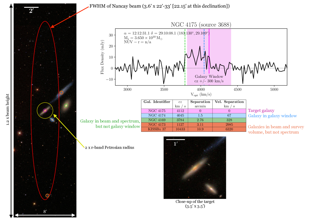
The Nançay telescope has a large beam which extends between in the N-S direction depending on the declination of the source. The change in the N-S beam width can be approximated by the polynomial
| (9) |
where is the beam width in arcminutes and is the declination in degrees (Matthews & van
Driel, 2000, Fig. 1.).
In this work, galaxies near the target source are considered as possible contaminators if
-
•
the secondary galaxy is located spatially within N-S half-power beam width and E-W half-power beam width, and
-
•
the redshift of the secondary galaxy is within of the target redshift.
A number of the target galaxies were found to have possible contaminators with very small angular separation distances. Upon inspection of the optical images for these sources, it was discovered that the possible contaminators were, in fact, part of the target galaxy. The SDSS pipeline has a known issue of de-blending large sources, particularly those with knots of star formation. In order not to over-classify the contaminant sources, a new criterion was therefore introduced to the search: the contaminant source must lie outside the edge of the target source, as defined as twice the -band Petrosian radius (), which according to Stoughton et al. (2002) is a good estimate of the size of the galaxy. Fig. 18 is an illustration of the method used to find any secondary contaminating sources.
Appendix C Defining a sample of H i non-detections
Appendix D Stacking NIBLES galaxies
D.1 Quantities measured from the stacked spectra
| Full Sample | Blue Sample | Red Sample | ||
| 1000 | 549 | 451 | N | |
| / | ||||
| S/N/ S/N | ||||
| All | () | |||
| 677 | 436 | 241 | N | |
| / | ||||
| S/N/ S/N | ||||
| Detections | () | |||
| 323 | 113 | 210 | N | |
| S/N/ S/N | ||||
| Non-detections | () | |||
| N | S/N | S/N | |||||
| Full Catalogue (all) | 521 | 277.7 | 205.7 | ||||
| Full Catalogue (blue) | 401 | 232.8 | 190.5 | ||||
| Full Catalogue (red) | 120 | 196.0 | 127.3 | ||||
| Non-detections (all) | 156 | 35.1 | 33.7 | ||||
| Non-detections (blue) | 97 | 29.5 | 28.1 | ||||
| Non-detections (red) | 59 | 11.1 | 7.5 |
| N | S/N | S/N | |||||
| Full Catalogue (all) | 479 | 54.2 | 172.6 | ||||
| Full Catalogue (blue) | 148 | 171.6 | 203.0 | ||||
| Full Catalogue (red) | 331 | 33.3 | 93.9 | ||||
| Non-detections (all) | 174 | 16.6 | 19.0 | ||||
| Non-detections (blue) | 17 | 12.1 | 10.8 | ||||
| Non-detections (red) | 157 | 8.0 | 16.0 |
D.2 Stacked Profiles for Fig. 9 and Fig. 10
Appendix E Catalogue of H i non-detections
| Source | RA | Dec | Name | ||||
|---|---|---|---|---|---|---|---|
| (J2000) | mag | mag | |||||
| CGCG 039-161 | |||||||
| PGC 1068442 | |||||||
| ASK 173829 | |||||||
| UGC 08986 | |||||||
| CGCG 019-019 | |||||||
| PGC 3124577 | |||||||
| NGC 2918 | |||||||
| NGC 3111 | |||||||
| NGC 5644 | |||||||
| NGC 5352 | |||||||
| NGC 0163 | |||||||
| NGC 3491 | |||||||
| UGC 07367 | |||||||
| NGC 4271 | |||||||
| UGC 09473 | |||||||
| NGC 4168 | |||||||
| NGC 4512 | |||||||
| NGC 3300 | |||||||
| NGC 4119 | |||||||
| NGC 4425 | |||||||
| NGC 4352 | |||||||
| NGC 4421 | |||||||
| NGC 5475 | |||||||
| NGC 4580 | |||||||
| NGC 4221 | |||||||
| NGC 3156 | |||||||
| NGC 3524 | |||||||
| NGC 3530 | |||||||
| NGC 4391 | |||||||
| NGC 4880 | |||||||
| NGC 4306 | |||||||
| NGC 3643 | |||||||
| NGC 4584 | |||||||
| NGC 4620 | |||||||
