On variational iterative methods for semilinear problems
Prosper Torsu

Department of Mathematics, California State University, Bakersfield, CA 93311, USA

Abstract

This paper presents an iterative method suitable for inverting semilinear problems which are important kernels in many numerical applications. The primary idea is to employ a parametrization that is able to reduce semilinear problems into linear systems which are solvable using fast Poisson solvers. Theoretical justifications are provided and supported by several experiments. Numerical results show that the method is not only computationally less expensive, but also yields accurate approximations.

Keywords: Finite element method, Adomian polynomials, Picard iteration

1 Introduction

The object of discussion in this article is an iterative procedure for inverting the semilinear problem

(aψ)+r(x,ψ)=f(x),xΩ,ψ(x)=0,xΩ,formulae-sequence𝑎𝜓𝑟x𝜓𝑓xformulae-sequencexΩformulae-sequence𝜓x0xΩ-\nabla\cdot(a\nabla\psi)+r(\textbf{x},\psi)=f(\textbf{x}),~{}~{}~{}~{}\textbf{x}\in\Omega,~{}~{}~{}~{}~{}~{}~{}\psi(\textbf{x})=0,~{}~{}~{}\textbf{x}\in\partial\Omega,\\ (1.1)

where ΩΩ\Omega is a bounded region with boundary ΩΩ\partial\Omega. The functions f𝑓f and g𝑔g are known continuous data and r:Ω×:𝑟Ωr:\Omega\times\mathbb{R}\to\mathbb{R} is continuously differentiable. In a variety of context, (1.1) is of great importance to mathematicians, physicists, biologists, engineers and other practitioners for modeling natural and human-induced phenomena. Models arising in this form describe steady-state characterization of evolution processes and have been the subject of extensive research in recent years. Some of the most commonly encountered classical mathematical models are prototypes of the differential equation in (1.1). They include the well-known Helmholtz equation, Bratu, Poisson-Boltzmann, the stationary Klein-Gordon, Allen-Cahn equation and Schrödinger equations. Precisely, applications arise in, but not limited to the study of electrostatic properties [5] and the study of acoustic and electromagnetic scattering [8, 16, 22]. In the sphere of fluid dynamics, some schemes (e.g. the Implicit Pressure, Explicit Saturation formulation of water-oil displacement [10]) are governed by variants of (1.1).

Indeed, simpler variations of (1.1) are separable in some coordinate systems, which allow solutions to be written in closed form. However, the fundamental models governing most natural phenomena involving motion, diffusion, reaction, etc. occur nonlinearly. Despite their pivotal contribution to the evolution of mathematical theories and experimentation, analytical methods have served minimal roles as only a handful of realistic models have known solutions. For several decades now, scientific computation has provided critical information about a wide class of problems that would otherwise be unavailable via analytical means. From a computational standpoint, solving (1.1) requires the simultaneous application of a numerical scheme with some sort of iterative procedure to an associated discrete algebraic system. As it is known, classical central and upwind schemes for the model problem (1.1) do not always produce satisfactory approximations. This is due to the inherent complex dynamics of r𝑟r leading to numerical challenges such as the appearance of singular effects [2, 19]. Even though these numerical tools are very successful, resolving instabilities for stable and accurate approximations often require a lot of computational time and large amounts of memory.

Ideally, analytical solutions to differential equations are desired. While this is possible when some components of the equation are trivialized, realistic models rarely admit closed form solutions. In recent years, advances in differential and integro-differential equations saw the light of novel analytical techniques [1, 3, 11, 23, 24]. The heart of these methods relies on perturbation arguments and the conjecture that solutions to nonlinear equations can be expressed as infinite series. This leads to a set of explicit recursive relations governing the modes of the series. Methods of this sort are robust and efficient for approximating solutions to IVPs, but have been modified to adapt to boundary and initial boundary-value problems. Certainly, the principal theme that has commanded most discussions about the aforementioned techniques is the rapid convergence of the series solutions. Despite this conception, important questions about the convergence of the method are still open because related studies are mainly problem-specific and do not provide a unifying ground to generalize results.

Far from a computational perspective is the issue of existence, solvability, uniqueness, regularity and number of solutions to (1.1). Nonlinear differential equations, in general, do not yield easily to rigorous and consolidated mathematical analysis. Successful investigations into the existence and uniqueness of solutions have relied on rigid assumption on a,r𝑎𝑟a,r and f𝑓f. In the notes [17], Naito investigated the existence of entire solutions by enforcing separability of r𝑟r in the spatial coordinates and the unknown. In particular, the form r=a(x)g(w)𝑟𝑎x𝑔𝑤r=a(\textbf{x})g(w) was assumed, where a𝑎a is locally Hölder on nsuperscript𝑛\mathbb{R}^{n} and f𝑓f is a locally Lipschitz continuous function on +superscript\mathbb{R}^{+} which is positive and nondecreasing for w>0𝑤0w>0. In the said article, the author established approximate range of the limit values of positive solutions. Naito’s results were later improved by Usami [21], where the general form r=g(x,w,w)𝑟𝑔x𝑤𝑤r=g(\textbf{x},w,\nabla w) was considered. A more general case was studied by Boccardo and co. [6]. Their study proved the existence and regularity of (1.1) with a non-constant conductivity and r=f(x)wγ𝑟𝑓xsuperscript𝑤𝛾r=f(\textbf{x})w^{-\gamma}, where γ>0𝛾0\gamma>0. The article concluded that a locally and strictly positive distributional solution to (1.1) exists if fL1(Ω)𝑓superscript𝐿1Ωf\in L^{1}(\Omega). A related discussion that runs across the aforementioned studies (also see [2, 4, 14]) is the existence of multiple nontrivial solutions even under very restrictive assumptions. Sometimes, infinitely many solutions exist [13, 18]. As much as extensive study of special classes of nonlinear differential equations exist today, there is no unified theory of nonlinear equations [20].

Inspired by the monographs [3, 15], this study presents an iterative procedure for approximating the solution, if it exists, to the variational equation associated with (1.1). The method is developed by employing a decomposition that is able to reduce the problem into a collection of sub-equations governed by the Laplacian. For compatible boundary conditions and domains, the method allows Fast Poisson Solvers to be used. The method extends to other boundary types trivially. Prescribing pure Dirichlet or Neumann boundary conditions is a matter of convenience and allows Fourier transforms to be used.

2 Variational formulation

Consider a bounded Lipschitz domain Ω2Ωsuperscript2\Omega\subset\mathbb{R}^{2} with polygonal boundary ΩΩ\partial\Omega. Let a:Ω+:𝑎Ωsuperscripta:\Omega\to\mathbb{R}^{+} with 0<amina(x)amax0subscript𝑎𝑎xsubscript𝑎0<a_{\min}\leq a(\textbf{x})\leq a_{\max} for all xΩxΩ\textbf{x}\in\Omega and define the usual Hilbert space

H01(Ω)={w:wL2(Ω),wL2(Ω) and w|Ω=0}.subscriptsuperscript𝐻10Ωconditional-set𝑤formulae-sequence𝑤superscript𝐿2Ω𝑤evaluated-atsuperscript𝐿2Ω and 𝑤Ω0H^{1}_{0}(\Omega)=\big{\{}w:w\in L^{2}(\Omega),~{}\nabla w\in L^{2}(\Omega)~{}\text{ and }~{}w|_{\partial\Omega}=0\big{\}}. (2.2)

Under the assumption that a solution (not necessarily unique) exists, given fL2(Ω)𝑓superscript𝐿2Ωf\in L^{2}(\Omega), the variational formulation associated with (1.1) reads:

Find uH01(Ω) satisfyingΩauwdA+Ωr(,u)wdA=ΩfwdA,wH01(Ω).formulae-sequenceFind uH01(Ω) satisfyingsubscriptΩ𝑎𝑢𝑤d𝐴subscriptΩ𝑟𝑢𝑤d𝐴subscriptΩ𝑓𝑤d𝐴for-all𝑤subscriptsuperscript𝐻10Ω\begin{split}&~{}\text{Find $u\in H^{1}_{0}(\Omega)$ satisfying}\\[4.30554pt] &\int_{\Omega}a\nabla u\cdot\nabla w\,\text{d}A+\int_{\Omega}r(\cdot,u)w\,\text{d}A=\int_{\Omega}fw\,\text{d}A,~{}~{}~{}\forall w\in H^{1}_{0}(\Omega).\end{split} (2.3)

In the sequel, the explicit dependence of r𝑟r on x is ignored and we write r(x,ψ)=r(ψ)𝑟x𝜓𝑟𝜓r(\textbf{x},\psi)=r(\psi) for brevity. An important step towards the construction of the finite element solution consists of approximating the continuous problem in (2.3) by seeking the solution on a finite dimensional subspace of H01(Ω)subscriptsuperscript𝐻10ΩH^{1}_{0}(\Omega). Mainly, H01(Ω)subscriptsuperscript𝐻10ΩH^{1}_{0}(\Omega) is replaced by the set of piecewise continuous polynomials with compact support.

2.1 Galerkin approximation

Consider a triangulation 𝒯hsubscript𝒯\mathcal{T}_{h} of ΩΩ\Omega such that Ω¯=τ𝒯hτ¯Ωsubscript𝜏subscript𝒯𝜏{\overline{\Omega}}=\cup_{\tau\in{\mathcal{T}}_{h}}\tau with h=maxτ𝒯h{hτ}subscript𝜏subscript𝒯subscript𝜏h=\max_{\tau\in{\mathcal{T}}_{h}}\{h_{\tau}\} and hτ=|τ|subscript𝜏𝜏h_{\tau}=\sqrt{|\tau|}. The finite element space associated with 𝒯hsubscript𝒯{\mathcal{T}}_{h} is defined as

𝒱h={whC(Ω¯):wh|τ is linear for all τ𝒯h, and wh|Ω=0}.subscript𝒱conditional-setsubscript𝑤𝐶¯Ωformulae-sequenceevaluated-atsubscript𝑤𝜏 is linear for all 𝜏subscript𝒯evaluated-at and subscript𝑤Ω0\mathcal{V}_{h}=\big{\{}w_{h}\in C(\overline{\Omega}):w_{h}|_{\tau}\text{ is linear for all }\tau\in\mathcal{T}_{h},\text{ and }w_{h}|_{\partial\Omega}=0\big{\}}. (2.4)

Then, the associated Galerkin finite element formulation is:

Find uh𝒱h satisfyingΩauhwhdA+Ωr(,uh)whdA=ΩfwhdA,wh𝒱h.formulae-sequenceFind uh𝒱h satisfyingsubscriptΩ𝑎subscript𝑢subscript𝑤d𝐴subscriptΩ𝑟subscript𝑢subscript𝑤d𝐴subscriptΩ𝑓subscript𝑤d𝐴for-allsubscript𝑤subscript𝒱\begin{split}&~{}\text{Find $u_{h}\in\mathcal{V}_{h}$ satisfying}\\[4.30554pt] &\int_{\Omega}a\nabla u_{h}\cdot\nabla w_{h}\,\text{d}A+\int_{\Omega}r(\cdot,u_{h})w_{h}\,\text{d}A=\int_{\Omega}fw_{h}\text{d}A,~{}~{}\forall w_{h}\in\mathcal{V}_{h}.\end{split} (2.5)

Let Z𝑍Z be the set of degrees of freedom associated with 𝒱hsubscript𝒱\mathcal{V}_{h} having |Z|=N~𝑍~𝑁|Z|=\widetilde{N}. Then,

𝒱h=span{ϕz}zZsubscript𝒱spansubscriptsubscriptitalic-ϕ𝑧𝑧𝑍\mathcal{V}_{h}=\text{span}\big{\{}\phi_{z}\big{\}}_{z\in Z} (2.6)

where ϕzsubscriptitalic-ϕ𝑧\phi_{z} is the finite element basis function tagged with the degree of freedom z𝑧z. By setting uh=zZαzϕzsubscript𝑢subscript𝑧𝑍subscript𝛼𝑧subscriptitalic-ϕ𝑧u_{h}=\sum_{z\in Z}\alpha_{z}\phi_{z}, the variational problem in (2.5) reduces to the following discrete algebraic equation governing 𝜶N~𝜶superscript~𝑁{\boldsymbol{\alpha}}\in\mathbb{R}^{\widetilde{N}}:

(𝜶)=𝒜𝜶+(𝜶)+𝜷=0,𝜶𝒜𝜶𝜶𝜷0\mathcal{R}({\boldsymbol{\alpha}})=\mathcal{A}{\boldsymbol{\alpha}}+\mathcal{B}({\boldsymbol{\alpha}})+{\boldsymbol{\beta}}=0, (2.7)

where 𝒜MN~×N~(),𝜷,N~\mathcal{A}\in M_{\widetilde{N}\times\widetilde{N}}(\mathbb{R}),~{}{\boldsymbol{\beta}},\in\mathbb{R}^{\widetilde{N}} and (𝜶)𝜶\mathcal{B}({\boldsymbol{\alpha}}) is a matrix function given by

𝒜ζz=ΩaϕzϕζdA,βζ=ΩfϕζdAandζ(𝜶)=Ωr(αzϕz)ϕζdA.formulae-sequencesubscript𝒜𝜁𝑧subscriptΩ𝑎subscriptitalic-ϕ𝑧subscriptitalic-ϕ𝜁d𝐴subscript𝛽𝜁subscriptΩ𝑓subscriptitalic-ϕ𝜁d𝐴andsubscript𝜁𝜶subscriptΩ𝑟subscript𝛼𝑧subscriptitalic-ϕ𝑧subscriptitalic-ϕ𝜁d𝐴\mathcal{A}_{\zeta z}=\int_{\Omega}a\nabla\phi_{z}\cdot\nabla\phi_{\zeta}\,\text{d}A,~{}~{}~{}~{}\beta_{\zeta}=\int_{\Omega}f\phi_{\zeta}\,\text{d}A~{}~{}~{}\text{and}~{}~{}~{}\mathcal{B}_{\zeta}({\boldsymbol{\alpha}})=\int_{\Omega}r(\sum\alpha_{z}\phi_{z})\phi_{\zeta}\,\text{d}A. (2.8)

respectively. The Galerkin solution that approximates ψ𝜓\psi is written

uh=zZαzϕz.subscript𝑢subscript𝑧𝑍subscript𝛼𝑧subscriptitalic-ϕ𝑧u_{h}=\sum_{z\in Z}\alpha_{z}\phi_{z}. (2.9)

As \mathcal{R} is nonlinear, direct inversion of (2.7) requires the use of some iterative scheme. Standard practice involves the application of quadrature rules alongside a linearization procedure. With appropriate regularity conditions, Newton methods guarantee higher convergence and are generally preferred. However, the laborious and unavoidable calculation of the associated Jacobian matrix makes Newton methods unappealing. Beside fixed point iterations, analytical methods have also been utilized to obtain qualitative features of solutions to nonlinear problems. Discussed in the next section is an iterative method which provides a general machinery for inverting (2.3).

3 An iterative approach

We furnish the weak form in (2.3) with a parametrization which transforms the variational problem into a sequential inversion of linear sub-problems. Suppose that ψ𝜓\psi and r𝑟r admit the decompositions

ψ=ζMψζandr=ζM𝒫ζformulae-sequence𝜓subscript𝜁𝑀subscript𝜓𝜁and𝑟subscript𝜁𝑀subscript𝒫𝜁\psi=\sum_{\zeta\leq M}\psi_{\zeta}~{}~{}~{}~{}\text{and}~{}~{}~{}~{}r=\sum_{\zeta\leq M}\mathcal{P}_{\zeta} (3.10)

where ψζ,0ζMsubscript𝜓𝜁0𝜁𝑀\psi_{\zeta},~{}0\leq\zeta\leq M, are to be determined. Here, construction of the set {𝒫ζ}ζMsubscriptsubscript𝒫𝜁𝜁𝑀\{\mathcal{P}_{\zeta}\}_{\zeta\leq M} is not well-defined, and thus, gives the reader the freedom to explore several possibilities. The construction adopted in this study engages sets of Adomian polynomials [11, 24] defined as

𝒫ζ=1(ζ1)!dζ1dλζ1[r(j0λjψj)]λ=0.subscript𝒫𝜁1𝜁1superscriptd𝜁1dsuperscript𝜆𝜁1subscriptdelimited-[]𝑟subscript𝑗0superscript𝜆𝑗subscript𝜓𝑗𝜆0\mathcal{P}_{\zeta}=\dfrac{1}{(\zeta-1)!}\dfrac{\textrm{d}^{\zeta-1}}{\textrm{d}\lambda^{\zeta-1}}\Big{[}r\Big{(}\sum_{j\geq 0}\lambda^{j}\psi_{j}\Big{)}\Big{]}_{\lambda=0}. (3.11)

This way, 𝒫ζsubscript𝒫𝜁\mathcal{P}_{\zeta} depends continuously on ψj,0jζ1subscript𝜓𝑗0𝑗𝜁1\psi_{j},~{}0\leq j\leq\zeta-1 only. Upon substituting (3.10) into (2.3), the variational equation can be written in the form

ζM(ΩaψζwdA+Ω𝒫ζwdA)=ΩfwdA.subscript𝜁𝑀subscriptΩ𝑎subscript𝜓𝜁𝑤d𝐴subscriptΩsubscript𝒫𝜁𝑤d𝐴subscriptΩ𝑓𝑤d𝐴\sum_{\zeta\leq M}\left(\int_{\Omega}a\nabla\psi_{\zeta}\cdot\nabla w\,\text{d}A+\int_{\Omega}\mathcal{P}_{\zeta}w\,\text{d}A\right)=\int_{\Omega}fw\,\text{d}A. (3.12)

The ultimate goal is to invert a set of linear sub-problems. Thus, the iterative scheme is developed by constructing the sequence {ψζ}ζMsubscriptsubscript𝜓𝜁𝜁𝑀\{\psi_{\zeta}\}_{\zeta\leq M} where the terms in (3.12) are associated such that ψζsubscript𝜓𝜁\psi_{\zeta} solves

Find ψζH01(Ω) satisfyingΩaψζwdA=(δζ01)Ω𝒫ζwdA+δζ0ΩfwdA,wH01(Ω).formulae-sequenceFind ψζH01(Ω) satisfyingsubscriptΩ𝑎subscript𝜓𝜁𝑤d𝐴subscript𝛿𝜁01subscriptΩsubscript𝒫𝜁𝑤d𝐴subscript𝛿𝜁0subscriptΩ𝑓𝑤d𝐴for-all𝑤subscriptsuperscript𝐻10Ω\begin{split}&~{}\text{Find $\psi_{\zeta}\in H^{1}_{0}(\Omega)$ satisfying}\\[4.30554pt] &\int_{\Omega}a\nabla\psi_{\zeta}\cdot\nabla w\,\text{d}A=(\delta_{\zeta 0}-1)\int_{\Omega}\mathcal{P}_{\zeta}w\,\text{d}A+\delta_{\zeta 0}\int_{\Omega}fw\,\text{d}A,~{}~{}~{}\forall w\in H^{1}_{0}(\Omega).\end{split} (3.13)

where δ𝛿\delta is the Kronecker delta. By construction, the term 𝒫ζsubscript𝒫𝜁\mathcal{P}_{\zeta} in the equation for ψζsubscript𝜓𝜁\psi_{\zeta} is known. Moreover, ψ0subscript𝜓0\psi_{0} absorbs the boundary conditions of the original problem. All higher order terms serve as corrections to the approximation ψ=ψ0𝜓subscript𝜓0\psi=\psi_{0} and honor the same boundary structure but homogeneous conditions. The practical solution is given by the (M+1)𝑀1(M+1)-term partial sum

ψM=ζMψζ.subscript𝜓𝑀subscript𝜁𝑀subscript𝜓𝜁\psi_{M}=\sum_{\zeta\leq M}\psi_{\zeta}. (3.14)

By requiring that 𝒫ζL2(Ω)subscript𝒫𝜁superscript𝐿2Ω\mathcal{P}_{\zeta}\in L^{2}(\Omega) for all 0ζM0𝜁𝑀0\leq\zeta\leq M, Lax-Milgram supplies the existence and uniqueness of each mode, and hence the partial solution. Because the decomposition is performed on the variational equation, the approach is applicable to other boundary types with equal success. Choosing pure Dirichlet or Neumann condition are means to facilitate the use of Fast Fourier Transforms.

Remark 3.1.

It is noteworthy that, as it is, this formulation may yield the trivial partial solution. Observe that, for a homogeneous equation, the zeroth mode solves ΩaψζwdA=0subscriptΩ𝑎subscript𝜓𝜁𝑤d𝐴0\int_{\Omega}a\nabla\psi_{\zeta}\cdot\nabla w\,\text{d}A=0 which yields the ψ0=0subscript𝜓00\psi_{0}=0 upon enforcing homogeneous boundary conditions. Largely, the zeroth mode inherits the most important qualitative features of the solution. As ψ0subscript𝜓0\psi_{0} deviates significantly, convergence is affected adversely. This can be avoided by introducing an auxiliary function gL2(Ω)𝑔superscript𝐿2Ωg\in L^{2}(\Omega) into the differential equation. For instance, one may rewrite the original equation (aψ)+r(x,ψ)=0𝑎𝜓𝑟x𝜓0-\nabla\cdot(a\nabla\psi)+r(\textbf{x},\psi)=0 as (aψ)+r~(x,ψ)=g(x)𝑎𝜓~𝑟x𝜓𝑔x-\nabla\cdot(a\nabla\psi)+\widetilde{r}(\textbf{x},\psi)=g(\textbf{x}), where r~(x,ψ)=r(x,ψ)+g(x)~𝑟𝑥𝜓𝑟x𝜓𝑔x\widetilde{r}(x,\psi)=r(\textbf{x},\psi)+g(\textbf{x}). This leads to a new set of polynomials {𝒫~ζ}ζMsubscriptsubscript~𝒫𝜁𝜁𝑀\{\widetilde{\mathcal{P}}_{\zeta}\}_{\zeta\leq M}, and a nontrivial solution zeroth mode available by solving Ωψ0wdA=ΩgwdAsubscriptΩsubscript𝜓0𝑤d𝐴subscriptΩ𝑔𝑤d𝐴\int_{\Omega}\nabla\psi_{0}\cdot\nabla w\,\text{d}A=\int_{\Omega}gw\,\text{d}A.

Contrary to fixed point methods, this approximation eliminates any form of linearization. The following results provide theoretical justifications which support stability of the modes and also establish convergence of (3.14).

Lemma 3.2.

For all ζM𝜁𝑀\zeta\leq M, the partial solution in (3.14) is stable provided 𝒫ζL2(Ω)subscript𝒫𝜁superscript𝐿2Ω\mathcal{P}_{\zeta}\in L^{2}(\Omega) for all  0ζM0𝜁𝑀0\leq\zeta\leq M.

Proof.

Stability of each mode is immediate since the weak forms in (3.13) possess unique solutions in H01(Ω)subscriptsuperscript𝐻10ΩH^{1}_{0}(\Omega) with

ψζ2δζ0Cζf2+(1δζ0)C~ζ𝒫ζ2,ζ=0,1,2,,M,formulae-sequencesubscriptnormsubscript𝜓𝜁2subscript𝛿𝜁0subscript𝐶𝜁subscriptnorm𝑓21subscript𝛿𝜁0subscript~𝐶𝜁subscriptnormsubscript𝒫𝜁2𝜁012𝑀\|\nabla{\psi}_{\zeta}\|_{2}\leq\delta_{\zeta 0}C_{\zeta}\|f\|_{2}+(1-\delta_{\zeta 0})\widetilde{C}_{\zeta}\|\mathcal{P}_{\zeta}\|_{2},~{}~{}~{}\zeta=0,1,2,\cdots,M,

where 2=(Ω||2dA)1/2\|\cdot\|_{2}=\left(\int_{\Omega}|\cdot|^{2}\,\text{d}A\right)^{1/2} and the constants Cζ,C~ζ,ζ=0,1,2formulae-sequencesubscript𝐶𝜁subscript~𝐶𝜁𝜁012C_{\zeta},\widetilde{C}_{\zeta},~{}\zeta=0,1,2\cdots are independent of ψζsubscript𝜓𝜁\psi_{\zeta}. It follows that

ψM2Cζf2+ζMC~ζ𝒫ζ2.subscriptnormsubscript𝜓𝑀2subscript𝐶𝜁subscriptnorm𝑓2subscript𝜁𝑀subscript~𝐶𝜁subscriptnormsubscript𝒫𝜁2\|\nabla\psi_{M}\|_{2}\leq C_{\zeta}\|f\|_{2}+\sum_{\zeta\leq M}\widetilde{C}_{\zeta}\|\mathcal{P}_{\zeta}\|_{2}.

This completes the proof. ∎

Lemma 3.3.

Let ψ𝜓\psi satisfy (2.3) and ψMsubscript𝜓𝑀\psi_{M} be the partial solution in (3.14). If 𝒫ζL2(Ω)subscript𝒫𝜁superscript𝐿2Ω\mathcal{P}_{\zeta}\in L^{2}(\Omega) for all 0ζM0𝜁𝑀0\leq\zeta\leq M, then (ψψM)20subscriptnorm𝜓subscript𝜓𝑀20\|\nabla(\psi-\psi_{M})\|_{2}\to 0 as M𝑀M\to\infty.

Proof.

By assumption, ψ𝜓\psi solves (2.3) and ψMsubscript𝜓𝑀\psi_{M} satisfies

ΩaψMwdA+ζMΩ𝒫ζwdA=ΩfwdA.subscriptΩ𝑎subscript𝜓𝑀𝑤d𝐴subscript𝜁𝑀subscriptΩsubscript𝒫𝜁𝑤d𝐴subscriptΩ𝑓𝑤d𝐴\int_{\Omega}a\nabla\psi_{M}\cdot\nabla w\,\text{d}A+\sum_{\zeta\leq M}\int_{\Omega}\mathcal{P}_{\zeta}w\,\text{d}A=\int_{\Omega}fw\,\text{d}A.

It follows that the error eM=ψψMsubscript𝑒𝑀𝜓subscript𝜓𝑀e_{M}=\psi-\psi_{M} satisfies

ΩaeMwdA=Ωr(ψ)wdAζMΩ𝒫ζwdA=ζ>MΩ𝒫ζwdA.subscriptΩ𝑎subscript𝑒𝑀𝑤d𝐴subscriptΩ𝑟𝜓𝑤d𝐴subscript𝜁𝑀subscriptΩsubscript𝒫𝜁𝑤d𝐴subscript𝜁𝑀subscriptΩsubscript𝒫𝜁𝑤d𝐴\begin{split}\int_{\Omega}a\nabla e_{M}\cdot\nabla w\,\text{d}A&=\int_{\Omega}r(\psi)w\,\text{d}A-\sum_{\zeta\leq M}\int_{\Omega}\mathcal{P}_{\zeta}w\,\text{d}A=\sum_{\zeta>M}\int_{\Omega}\mathcal{P}_{\zeta}w\,\text{d}A.\end{split}

From Cauchy-Schwarz, Poincaré and triangle inequalities, it holds that

eM22(ζ>M𝒫ζ2)eM2(ζ>M𝒫ζ2)eM2.subscriptsuperscriptdelimited-∥∥subscript𝑒𝑀22subscript𝜁𝑀subscriptdelimited-∥∥subscript𝒫𝜁2subscriptdelimited-∥∥subscript𝑒𝑀2subscript𝜁𝑀subscriptdelimited-∥∥subscript𝒫𝜁2subscriptdelimited-∥∥subscript𝑒𝑀2\begin{split}\|\nabla e_{M}\|^{2}_{2}&\leq\Bigg{(}\sum_{\zeta>M}\|\mathcal{P}_{\zeta}\|_{2}\Bigg{)}\|e_{M}\|_{2}\leq\Bigg{(}\sum_{\zeta>M}\|\mathcal{P}_{\zeta}\|_{2}\Bigg{)}\|\nabla e_{M}\|_{2}.\end{split}

Consequently,

eM2ζ>M𝒫ζ2.subscriptnormsubscript𝑒𝑀2subscript𝜁𝑀subscriptnormsubscript𝒫𝜁2\|\nabla e_{M}\|_{2}\leq\sum_{\zeta>M}\|\mathcal{P}_{\zeta}\|_{2}. (3.15)

The theorem follows as ζ>M𝒫ζ0subscript𝜁𝑀subscript𝒫𝜁0\sum_{\zeta>M}\mathcal{P}_{\zeta}\to 0 for sufficiently large M𝑀M. ∎

3.1 Comparison with Picard iteration

The iterative method discussed above shares some similarities with Picard Iteration, where each iteration solves a linear problem. For the form in (2.3), the fixed point iteration is:

Algorithm 1 Picard iteration
1:Set an initial iterate ψ(0)H01(Ω)superscript𝜓0subscriptsuperscript𝐻10Ω\psi^{(0)}\in H^{1}_{0}(\Omega).
2:for M=0,1,𝑀01M=0,1,\cdots do
3:     Find ψ(M+1)H01(Ω)superscript𝜓𝑀1subscriptsuperscript𝐻10Ω\psi^{(M+1)}\in H^{1}_{0}(\Omega) satisfying
4:     Ωaψ(M+1)wdA=ΩfwdAΩr(ψ(M))wdA,wH01(Ω).formulae-sequencesubscriptΩ𝑎superscript𝜓𝑀1𝑤d𝐴subscriptΩ𝑓𝑤d𝐴subscriptΩ𝑟superscript𝜓𝑀𝑤d𝐴for-all𝑤subscriptsuperscript𝐻10Ω\displaystyle\int_{\Omega}a\nabla\psi^{(M+1)}\cdot\nabla w\,\text{d}A=\int_{\Omega}fw\,\text{d}A-\int_{\Omega}r(\psi^{(M)})w\,\text{d}A,~{}~{}~{}\forall w\in H^{1}_{0}(\Omega).
5:end for

In fact, Lemma 3.4 shows that if r𝑟r is linear and the set {𝒫ζ}ζ0subscriptsubscript𝒫𝜁𝜁0\{\mathcal{P}_{\zeta}\}_{\zeta\geq 0} is constructed according to (3.11), the two schemes are identical.

Lemma 3.4.

Let ψMsubscript𝜓𝑀\psi_{M} and ψ(M)superscript𝜓𝑀\psi^{(M)} be the Mthsuperscript𝑀thM^{\text{th}} iterate of the procedure above and Picard iteration respectively. Assume that r𝑟r is linear and {𝒫ζ}ζ0subscriptsubscript𝒫𝜁𝜁0\{\mathcal{P}_{\zeta}\}_{\zeta\geq 0} is constructed according to (3.11). If ψ0=ψ(0)subscript𝜓0superscript𝜓0\psi_{0}=\psi^{(0)}, then ψM=ψ(M)subscript𝜓𝑀superscript𝜓𝑀\psi_{M}=\psi^{(M)} holds for all M1𝑀1M\geq 1.

Proof.

The argument is inductive. Since r𝑟r is linear, we must have 𝒫ζ=r(ψζ)=ψζsubscript𝒫𝜁𝑟subscript𝜓𝜁subscript𝜓𝜁\mathcal{P}_{\zeta}=r(\psi_{\zeta})=\psi_{\zeta}. Thus,

ΩaψMwdA=ΩfwdAζMΩ𝒫ζwdA=ΩfwdAΩψM1wdA.subscriptΩ𝑎subscript𝜓𝑀𝑤d𝐴subscriptΩ𝑓𝑤d𝐴subscript𝜁𝑀subscriptΩsubscript𝒫𝜁𝑤d𝐴subscriptΩ𝑓𝑤d𝐴subscriptΩsubscript𝜓𝑀1𝑤d𝐴\begin{split}\int_{\Omega}a\nabla\psi_{M}\cdot\nabla w\,\text{d}A&=\int_{\Omega}fw\,\text{d}A-\sum_{\zeta\leq M}\int_{\Omega}\mathcal{P}_{\zeta}w\,\text{d}A\\ &=\int_{\Omega}fw\,\text{d}A-\int_{\Omega}\psi_{M-1}w\,\text{d}A.\end{split} (3.16)

From algorithm 1, ψ(M)superscript𝜓𝑀\psi^{(M)} also satisfies

Ωaψ(M)wdA=ΩfwdAΩψ(M1)wdA.subscriptΩ𝑎superscript𝜓𝑀𝑤d𝐴subscriptΩ𝑓𝑤d𝐴subscriptΩsuperscript𝜓𝑀1𝑤d𝐴\int_{\Omega}a\nabla\psi^{(M)}\cdot\nabla w\,\text{d}A=\int_{\Omega}fw\,\text{d}A-\int_{\Omega}\psi^{(M-1)}w\,\text{d}A.\\ (3.17)

Suppose for the sake of induction that ψ(M1)=ψM1superscript𝜓𝑀1subscript𝜓𝑀1\psi^{(M-1)}=\psi_{M-1} for M2𝑀2M\geq 2. It follows from (3.17) and (3.16) that

Ωa(ψMψ(M))wdA=Ω(ψ(M1)ψM1)wdA.subscriptΩ𝑎subscript𝜓𝑀superscript𝜓𝑀𝑤d𝐴subscriptΩsuperscript𝜓𝑀1subscript𝜓𝑀1𝑤d𝐴\begin{split}\int_{\Omega}a\nabla(\psi_{M}-\psi^{(M)})\cdot\nabla w\,\text{d}A&=\int_{\Omega}\left(\psi^{(M-1)}-\psi_{M-1}\right)w\,\text{d}A.\end{split}

The last equation is zero by assumption. As this holds for arbitrary wH01(Ω)𝑤subscriptsuperscript𝐻10Ωw\in H^{1}_{0}(\Omega), it must be that ψ(M)ψMsuperscript𝜓𝑀subscript𝜓𝑀\psi^{(M)}-\psi_{M} is constant in H01(Ω)subscriptsuperscript𝐻10ΩH^{1}_{0}(\Omega). We then deduce that ψ(M)ψM=0superscript𝜓𝑀subscript𝜓𝑀0\psi^{(M)}-\psi_{M}=0. ∎

Equation (3.15) shows that convergence of the partial solution is controlled by the rate of decay of 𝒫ζsubscript𝒫𝜁\mathcal{P}_{\zeta}. Certainly, this procedure is attractive because, similar to Picard iteration, calculation of the Jacobian associated with (2.7) is replaced by the repeated inversion of the operator (a)\nabla\cdot(a\nabla\cdot). Since the computational cost of inverting a single instance of this operator on a highly resolved mesh can be enormous for traditional numerical methods, calculation of (3.14) is highly prohibitive for large M𝑀M. More importantly, engagement of Fast Poisson Solvers is limited because symmetry of the resulting stiffness matrix coefficients is affected.

In what follows, we reduce (3.13) into variational sub-problems governed by a~(x)=1~𝑎x1\widetilde{a}(\textbf{x})=1 for all x. This allows us to employ discrete sine transforms to accelerate calculation of the modes. To accomplish this, consider the conductivity log characterization [9]

𝒴=loga,𝒴𝑎\mathcal{Y}=\log a, (3.18)

which exists, and is defined since a(x)>0𝑎x0a(\textbf{x})>0 for all xΩxΩ\textbf{x}\in\Omega. This suggests that for sufficiently large N𝑁N, a𝑎a can be approximated using the truncated Taylor series

a=ξN𝒴ξ/ξ!.𝑎subscript𝜉𝑁superscript𝒴𝜉𝜉a=\sum_{\xi\leq N}\mathcal{Y}^{\xi}/\xi!. (3.19)

Using this representation for a fixed ζ𝜁\zeta, the variational equation in (3.13) becomes

ξN1ξ!Ω𝒴ξψζξwdA=(δζ01)Ω𝒫ζwdA+δζ0ΩfwdA.subscript𝜉𝑁1𝜉subscriptΩsuperscript𝒴𝜉subscript𝜓𝜁𝜉𝑤d𝐴subscript𝛿𝜁01subscriptΩsubscript𝒫𝜁𝑤d𝐴subscript𝛿𝜁0subscriptΩ𝑓𝑤d𝐴\sum_{\xi\leq N}\frac{1}{\xi!}\int_{\Omega}\mathcal{Y}^{\xi}\nabla\psi_{\zeta\xi}\cdot\nabla w\,\text{d}A=(\delta_{\zeta 0}-1)\int_{\Omega}\mathcal{P}_{\zeta}w\,\text{d}A+\delta_{\zeta 0}\int_{\Omega}fw\,\text{d}A. (3.20)

By collecting terms of the same order (index of ψζsubscript𝜓𝜁\psi_{\zeta} and the exponent of 𝒴𝒴\mathcal{Y} adds up to the same n𝑛n\in\mathbb{N}), (3.21) transforms into the following recursive equations:

Ωψζ0wdA=(δζ01)Ω𝒫ζwdA+δζ0ΩfwdA,ΩψζξwdA+j=1ξ1j!Ω𝒴jψζ,ξjwdA=0,ξ1.formulae-sequencesubscriptΩsubscript𝜓𝜁0𝑤d𝐴subscript𝛿𝜁01subscriptΩsubscript𝒫𝜁𝑤d𝐴subscript𝛿𝜁0subscriptΩ𝑓𝑤d𝐴formulae-sequencesubscriptΩsubscript𝜓𝜁𝜉𝑤d𝐴superscriptsubscript𝑗1𝜉1𝑗subscriptΩsuperscript𝒴𝑗subscript𝜓𝜁𝜉𝑗𝑤d𝐴0𝜉1\begin{split}&\int_{\Omega}\nabla\psi_{\zeta 0}\cdot\nabla w\,\text{d}A=(\delta_{\zeta 0}-1)\int_{\Omega}\mathcal{P}_{\zeta}w\,\text{d}A+\delta_{\zeta 0}\int_{\Omega}fw\,\text{d}A,\\[8.61108pt] &\int_{\Omega}\nabla\psi_{\zeta\xi}\cdot\nabla w\,\text{d}A+\sum_{j=1}^{\xi}\frac{1}{j!}\int_{\Omega}\mathcal{Y}^{j}\nabla\psi_{\zeta,\xi-j}\cdot\nabla w\,\text{d}A=0,~{}~{}\xi\geq 1.\end{split} (3.21)

The approximate solution is written as

ψMN=ζMξNψζξ.subscript𝜓𝑀𝑁subscript𝜁𝑀subscript𝜉𝑁subscript𝜓𝜁𝜉\psi_{MN}=\sum_{\zeta\leq M}\sum_{\xi\leq N}\psi_{\zeta\xi}. (3.22)

Clearly, any unfavorable effect of a𝑎a on the invertibility of the resulting stiffness matrix is avoided. A minimal penalty is realized in the calculation of the load vector.

3.2 Discrete algorithm

The procedure discussed in the preceding sections can be summarized as follows:

Algorithm 2 Series approximation
1:Fix M,N𝑀𝑁M,N.
2:for ζ=0𝜁0\zeta=0 to N𝑁N do
3:     for ξ=0𝜉0\xi=0 to M𝑀M do
4:         Find ψζ0𝒱h:Ωψζ0wdA=δζ0ΩfwdAδξ0Ω𝒫ζwdA:subscript𝜓𝜁0subscript𝒱subscriptΩsubscript𝜓𝜁0𝑤d𝐴subscript𝛿𝜁0subscriptΩ𝑓𝑤d𝐴subscript𝛿𝜉0subscriptΩsubscript𝒫𝜁𝑤d𝐴\displaystyle\psi_{\zeta 0}\in\mathcal{V}_{h}:\int_{\Omega}\nabla\psi_{\zeta 0}\cdot\nabla w\,\text{d}A=\delta_{\zeta 0}\int_{\Omega}fw\,\text{d}A-\delta_{\xi 0}\int_{\Omega}\mathcal{P}_{\zeta}w\,\text{d}A
5:         Find ψζξ𝒱h:ΩψζξwdA+jξ1j!Ω𝒴jψζ,ξjwdA=0,ζ,ξ1:subscript𝜓𝜁𝜉subscript𝒱formulae-sequencesubscriptΩsubscript𝜓𝜁𝜉𝑤d𝐴subscript𝑗𝜉1𝑗subscriptΩsuperscript𝒴𝑗subscript𝜓𝜁𝜉𝑗𝑤d𝐴0𝜁𝜉1\displaystyle\psi_{\zeta\xi}\in\mathcal{V}_{h}:\int_{\Omega}\nabla\psi_{\zeta\xi}\cdot\nabla w\,\text{d}A+\sum_{j\leq\xi}\frac{1}{j!}\int_{\Omega}\mathcal{Y}^{j}\nabla\psi_{\zeta,\xi-j}\cdot\nabla w\,\text{d}A=0,~{}~{}\zeta,\xi\geq 1
6:     end for
7:end for
8:Set ψMN=ζMξNψζξsubscript𝜓𝑀𝑁subscript𝜁𝑀subscript𝜉𝑁subscript𝜓𝜁𝜉\psi_{MN}=\sum_{\zeta\leq M}\sum_{\xi\leq N}\psi_{\zeta\xi}.

For all ζ𝜁\zeta, we can verify that the variational problems in Algorithm 2 have unique solutions in H01(Ω)subscriptsuperscript𝐻10ΩH^{1}_{0}(\Omega) satisfying the following stability estimate:

ψζ02Cζ0(δζ0f2+𝒫ζ2)subscriptnormsubscript𝜓𝜁02subscript𝐶𝜁0subscript𝛿𝜁0subscriptnorm𝑓2subscriptnormsubscript𝒫𝜁2\|\nabla\psi_{\zeta 0}\|_{2}\leq C_{\zeta 0}\left(\delta_{\zeta 0}\|f\|_{2}+\|\mathcal{P}_{\zeta}\|_{2}\right) (3.23)

provided 𝒫ζL2(Ω)subscript𝒫𝜁superscript𝐿2Ω\mathcal{P}_{\zeta}\in L^{2}(\Omega). By construction, Ωψζ1wdA+Ω𝒴ψζ0wdA=0subscriptΩsubscript𝜓𝜁1𝑤d𝐴subscriptΩ𝒴subscript𝜓𝜁0𝑤d𝐴0\int_{\Omega}\nabla\psi_{\zeta 1}\cdot\nabla w\,\text{d}A+\int_{\Omega}\mathcal{Y}\nabla\psi_{\zeta 0}\cdot\nabla w\,\text{d}A=0. Thus, as long as 𝒴L2(Ω)𝒴superscript𝐿2Ω\mathcal{Y}\in L^{2}(\Omega), it follows that

ψζ12𝒴2ψζ02Cζ1𝒴2(δζ0f2+𝒫ζ2).subscriptdelimited-∥∥subscript𝜓𝜁12subscriptdelimited-∥∥𝒴2subscriptdelimited-∥∥subscript𝜓𝜁02subscript𝐶𝜁1subscriptdelimited-∥∥𝒴2subscript𝛿𝜁0subscriptdelimited-∥∥𝑓2subscriptdelimited-∥∥subscript𝒫𝜁2\begin{split}\|\nabla\psi_{\zeta 1}\|_{2}&\leq\|\mathcal{Y}\|_{2}\|\nabla\psi_{\zeta 0}\|_{2}\\ &\leq C_{\zeta 1}\|\mathcal{Y}\|_{2}\left(\delta_{\zeta 0}\|f\|_{2}+\|\mathcal{P}_{\zeta}\|_{2}\right).\end{split}

By complete induction, we have

ψζξ2Cζξ𝒴2ξ(δζ0f2+𝒫ζ2).subscriptnormsubscript𝜓𝜁𝜉2subscript𝐶𝜁𝜉subscriptsuperscriptnorm𝒴𝜉2subscript𝛿𝜁0subscriptnorm𝑓2subscriptnormsubscript𝒫𝜁2\|\nabla\psi_{\zeta\xi}\|_{2}\leq C_{\zeta\xi}\|\mathcal{Y}\|^{\xi}_{2}\left(\delta_{\zeta 0}\|f\|_{2}+\|\mathcal{P}_{\zeta}\|_{2}\right).\\ (3.24)

Upon a successful Galerkin discretization, the discrete equations have the form 𝒛=𝒛\mathcal{M}{\boldsymbol{z}}=\mathcal{F} where \mathcal{M} is the discrete Laplacian. The collection can now be solved efficiently and fast using the fast Poisson solver discussed in the next section. As much as the summation in the equation for ψζξsubscript𝜓𝜁𝜉\psi_{\zeta\xi} tells a strong dependence of higher-order terms on lower-order ones, Fast Poisson solvers comes in handy especially when a lot of terms are required to represent each mode accurately.

For Neumann problems, the Galerkin discretization is known to produce a linear system characterized by a one-dimensional kernel. The associated stiffness matrix is singular with fatal effects on iterative solvers, e.g., conjugate gradient. Often, the kernel is eliminated by specifying data at a particular node, or approximate the system using a minimization-based iterative solver [7]. While these techniques seemingly avert direct inversion a singular matrix, Bochev and co., in the referenced article, remarked that such choices are subtle and unsatisfactory because specifying data at a specific node is ambivalent and roundoff errors may hinder convergence of the iterative solver. In this context, Algorithm 2 provides the environment to exploit direct solvers.

In very limited cases, (1.1) is fast solvable on simple geometries. The most common numerical treatment of the finite element discretization involves a uniform mesh refinement across the entire computational domain. This poses numerical challenges as the finite element method (as well as finite difference and finite volume) performs poorly with vanishing element width. For the prescribed boundary conditions, this is no longer a limitation because we are able to use Fourier transforms to invert the sub-systems efficiently.

4 A Fast Poisson Solver (FPS)

Fast Poisson Solvers are simple but powerful machinery which harness Fourier transforms to produce efficient solvers for the Poisson equation with compatible boundary conditions. They require a low amount of arithmetic operations and can be executed effectively with optimal operation count of 𝒪(n2logn)𝒪superscript𝑛2𝑛\mathcal{O}(n^{2}\log n). The procedure that utilizes finite difference is discussed in [12]. Let 𝒛=𝒛\mathcal{M}{\boldsymbol{z}}=\mathcal{F} be the algebraic system resulting from the Galerkin approximation of

ΩzwdA=ΩgwdAsubscriptΩ𝑧𝑤d𝐴subscriptΩ𝑔𝑤d𝐴\int_{\Omega}\nabla z\cdot\nabla w\,\text{d}A=\int_{\Omega}gw\,\text{d}A

using the bilinear basis. Then \mathcal{M} consists of block diagonal matrices identified as TST (Toeplitz, Symmetric and Tridiagonal). Denote by TD(n;α,β)𝑛superscript𝛼superscript𝛽(n;\alpha^{\star},\beta^{\star}) the n×n𝑛𝑛n\times n tridiagonal matrix with αsuperscript𝛼\alpha^{\star} along the principal diagonal and βsuperscript𝛽\beta^{\star} along the sub- and super-diagonals. For the finite element discretization, let ΔxΔ𝑥\Delta x and ΔyΔ𝑦\Delta y be the element width with n1subscript𝑛1n_{1} and n2subscript𝑛2n_{2} elements in the vertical and lateral directions respectively. Then =absent\mathcal{M}= TD(n;𝒮,𝒯)𝑛𝒮𝒯(n;\mathcal{S},\mathcal{T}), where 𝒮𝒮\mathcal{S} and 𝒯𝒯\mathcal{T} are themselves TST with sub- and super-diagonals

𝒮ii=43ΔxΔy(Δx2+Δy2),𝒮i1,i=𝒮i,i+1=13ΔxΔy(Δx22Δy2),𝒯ii=13ΔxΔy(Δx22Δy2),𝒯i1,i=𝒯i,i+1=16ΔxΔy(Δx2+Δy2).\begin{split}\mathcal{S}_{ii}&=\frac{4}{3\Delta x\Delta y}\,(\Delta x^{2}+\Delta y^{2}),\hskip 16.62178pt\mathcal{S}_{i-1,i}=\mathcal{S}_{i,i+1}=\frac{1}{3\Delta x\Delta y}(\Delta x^{2}-2\Delta y^{2}),\\[8.61108pt] \mathcal{T}_{ii}&=\frac{1}{3\Delta x\Delta y}(\Delta x^{2}-2\Delta y^{2}),\hskip 14.45377pt\mathcal{T}_{i-1,i}=\mathcal{T}_{i,i+1}=-\frac{1}{6\Delta x\Delta y}(\Delta x^{2}+\Delta y^{2}).\end{split} (4.25)

Interestingly, TST matrices encode critical information which are fundamental to the implementation of FFT-based Poisson solvers. In fact, the linear system 𝒛=𝒛\mathcal{M}{\boldsymbol{z}}=\mathcal{F} is solvable completely by using the eigenvalues and eigenfunctions of 𝒮𝒮\mathcal{S} and 𝒯𝒯\mathcal{T} only. First, the eigenvectors are given explicitly by the formula

φjl=2n1+1sin(πjln1+1),j,l=1,2,,n1.formulae-sequencesubscript𝜑𝑗𝑙2subscript𝑛11𝜋𝑗𝑙subscript𝑛11𝑗𝑙12subscript𝑛1\varphi_{jl}=\sqrt{\frac{2}{n_{1}+1}}\sin\Big{(}\frac{\pi jl}{n_{1}+1}\Big{)},~{}~{}~{}j,l=1,2,\cdots,n_{1}. (4.26)

Moreover, the collection {φjl}jl=1n1superscriptsubscriptsubscript𝜑𝑗𝑙𝑗𝑙1subscript𝑛1\{\varphi_{jl}\}_{jl=1}^{n_{1}} is orthonormal with corresponding eigenvalues

λj𝒮=43(ΔxΔy+ΔyΔx)+23(ΔxΔy2ΔyΔx)cos(πjn1+1),λj𝒯=13(ΔyΔx2ΔxΔy)13(ΔxΔy+ΔyΔx)cos(πjn1+1).formulae-sequencesuperscriptsubscript𝜆𝑗𝒮43Δ𝑥Δ𝑦Δ𝑦Δ𝑥23Δ𝑥Δ𝑦2Δ𝑦Δ𝑥𝜋𝑗subscript𝑛11superscriptsubscript𝜆𝑗𝒯13Δ𝑦Δ𝑥2Δ𝑥Δ𝑦13Δ𝑥Δ𝑦Δ𝑦Δ𝑥𝜋𝑗subscript𝑛11\begin{split}\lambda_{j}^{\mathcal{S}}&=\frac{4}{3}\left(\frac{\Delta x}{\Delta y}+\frac{\Delta y}{\Delta x}\right)+\frac{2}{3}\left(\frac{\Delta x}{\Delta y}-\frac{2\Delta y}{\Delta x}\right)\cos\Big{(}\frac{\pi j}{n_{1}+1}\Big{)},\\[12.91663pt] \lambda_{j}^{\mathcal{T}}&=\frac{1}{3}\left(\frac{\Delta y}{\Delta x}-\frac{2\Delta x}{\Delta y}\right)-\frac{1}{3}\left(\frac{\Delta x}{\Delta y}+\frac{\Delta y}{\Delta x}\right)\cos\Big{(}\frac{\pi j}{n_{1}+1}\Big{)}.\end{split} (4.27)

With the set {φjl,λj𝒮,λj𝒯}jl=1n1superscriptsubscriptsubscript𝜑𝑗𝑙superscriptsubscript𝜆𝑗𝒮superscriptsubscript𝜆𝑗𝒯𝑗𝑙1subscript𝑛1\{\varphi_{jl},\lambda_{j}^{\mathcal{S}},\lambda_{j}^{\mathcal{T}}\}_{jl=1}^{n_{1}} available, construction of the fast Poisson solver is straightforward. Let 𝒛=(𝒛1,𝒛2,,𝒛n2)T𝒛superscriptsubscript𝒛1subscript𝒛2subscript𝒛subscript𝑛2𝑇\boldsymbol{z}=(\boldsymbol{z}_{1},\boldsymbol{z}_{2},\cdots,\boldsymbol{z}_{n_{2}})^{T} and =(𝒬1,𝒬2,,𝒬n2)Tsuperscriptsubscript𝒬1subscript𝒬2subscript𝒬subscript𝑛2𝑇\mathcal{F}=(\mathcal{Q}_{1},\mathcal{Q}_{2},\cdots,\mathcal{Q}_{n_{2}})^{T} where 𝒛lsubscript𝒛𝑙\boldsymbol{z}_{l} and 𝒬lsubscript𝒬𝑙\mathcal{Q}_{l} are block vectors corresponding to the lthsuperscript𝑙thl^{\text{th}} column of \mathcal{M} and \mathcal{F} respectively. Then 𝒛=𝒛\mathcal{M}{\boldsymbol{z}}=\mathcal{F} is expressible as

𝒯𝒛l1+𝒮𝒛l+𝒯𝒛l+1=𝒬l,l=1,2,,n2.formulae-sequence𝒯subscript𝒛𝑙1𝒮subscript𝒛𝑙𝒯subscript𝒛𝑙1subscript𝒬𝑙𝑙12subscript𝑛2\mathcal{T}\boldsymbol{z}_{l-1}+\mathcal{S}\boldsymbol{z}_{l}+\mathcal{T}\boldsymbol{z}_{l+1}=\mathcal{Q}_{l},~{}~{}l=1,2,\cdots,n_{2}. (4.28)

Denote by ΦΦ\Phi the matrix whose (jl)thsuperscript𝑗𝑙th(jl)^{\text{th}} entry is given by (4.26). Then

𝒮=ΦD𝒮ΦTand𝒯=ΦD𝒯ΦT,𝒮Φsubscript𝐷𝒮superscriptΦ𝑇and𝒯Φsubscript𝐷𝒯superscriptΦ𝑇\mathcal{S}=\Phi D_{\mathcal{S}}\Phi^{T}~{}~{}~{}\text{and}~{}~{}~{}\mathcal{T}=\Phi D_{\mathcal{T}}\Phi^{T},

where D=diag[λl,λl,,λl]subscript𝐷diagsuperscriptsubscript𝜆𝑙superscriptsubscript𝜆𝑙superscriptsubscript𝜆𝑙D_{\mathcal{I}}=\text{diag}[\lambda_{l}^{\mathcal{I}},\lambda_{l}^{\mathcal{I}},\cdots,\lambda_{l}^{\mathcal{I}}]. Orthogonality of ΦΦ\Phi implies that (4.28) can be reduced to

D𝒯𝜻l1+D𝒮𝜻l+D𝒯𝜻l+1=𝝃l,l=1,2,,n2,formulae-sequencesubscript𝐷𝒯subscript𝜻𝑙1subscript𝐷𝒮subscript𝜻𝑙subscript𝐷𝒯subscript𝜻𝑙1subscript𝝃𝑙𝑙12subscript𝑛2D_{\mathcal{T}}\boldsymbol{\zeta}_{l-1}+D_{\mathcal{S}}\boldsymbol{\zeta}_{l}+D_{\mathcal{T}}\boldsymbol{\zeta}_{l+1}=\boldsymbol{\xi}_{l},~{}~{}~{}l=1,2,\cdots,n_{2}, (4.29)

where, Φ𝒛l=𝜻lΦsubscript𝒛𝑙subscript𝜻𝑙\Phi\boldsymbol{z}_{l}=\boldsymbol{\zeta}_{l} and Φ𝒬l=𝝃lΦsubscript𝒬𝑙subscript𝝃𝑙\Phi\mathcal{Q}_{l}=\boldsymbol{\xi}_{l}. These operations successfully decoupled 𝒛=𝒛\mathcal{M}{\boldsymbol{z}}=\mathcal{F} into a set of independent one-dimensional tridiagonal systems which can be solved using fast tridiagonal solvers.

5 Numerical Tests

We present three numerical tests to explore the effect of M𝑀M and N𝑁N on the accuracy of the series approximations. Even though the problems are manufactured and may not bear any physical meaning, they do provide good insights into the performance of the method. Because of the close similarity, we also compute reference approximations by direct simulation of (𝜶)=𝟎𝜶0\mathcal{R}({\boldsymbol{\alpha}})={\boldsymbol{0}} using Picard iteration. The stopping criterion is (𝜶)1010subscriptnorm𝜶superscript1010\|\mathcal{R}({\boldsymbol{\alpha}})\|_{\infty}\leq 10^{-10}.

5.1 Test 1

: In this foremost experiment, we set a(x1,x2)=1,r(ψ)=ψψ3formulae-sequence𝑎subscript𝑥1subscript𝑥21𝑟𝜓𝜓superscript𝜓3a(x_{1},x_{2})=1,~{}r(\psi)=\psi-\psi^{3} and f𝑓f is chosen appropriately so that (1.1) admits the solution ψ(x1,x2)=ω(x1)ω(x2)𝜓subscript𝑥1subscript𝑥2𝜔subscript𝑥1𝜔subscript𝑥2\psi(x_{1},x_{2})=\omega(x_{1})\omega(x_{2}), where

ω(s)=1+exp(1/0.05)exp(s/0.05)exp((s1)/0.05).𝜔𝑠110.05𝑠0.05𝑠10.05\omega(s)=1+\exp(-1/0.05)-\exp(-s/0.05)-\exp((s-1)/0.05).

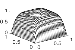
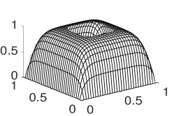
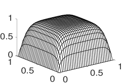
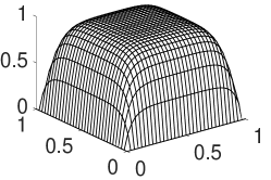
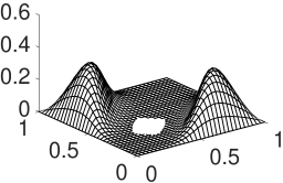
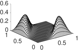
Since a𝑎a is constant, the index ξ𝜉\xi is redundant. Thus, we simply denote ψζξsubscript𝜓𝜁𝜉\psi_{\zeta\xi} by ψζsubscript𝜓𝜁\psi_{\zeta}. Figure 1 compares the numerical approximations of ψ1,ψ4subscript𝜓1subscript𝜓4\psi_{1},\psi_{4} and ψ8subscript𝜓8\psi_{8} with the analytical solution.

Refer to caption

(a) ψ1subscript𝜓1\psi_{1} approximation

Refer to caption

(b) ψ4subscript𝜓4\psi_{4} approximation

Refer to caption

(c) ψ8subscript𝜓8\psi_{8} approximation

Refer to caption

(d) Analytical solution
Figure 1: Approximation of various modes compared with the analytical solution.
Number of elements
23×23superscript23superscript23~{}~{}2^{3}\times 2^{3} 24×24superscript24superscript24~{}~{}2^{4}\times 2^{4}~{} 25×25superscript25superscript25~{}~{}2^{5}\times 2^{5}~{} 26×26superscript26superscript26~{}~{}2^{6}\times 2^{6}~{} 27×27superscript27superscript27~{}~{}2^{7}\times 2^{7}
M=1𝑀1M=1 3.80095(01)3.80095013.80095(-01) 9.56161(02)9.56161029.56161(-02) 2.99741(02)2.99741022.99741(-02) 1.41233(02)1.41233021.41233(-02) 1.02027(02)1.02027021.02027(-02)
M=3𝑀3M=3 3.88708(01)3.88708013.88708(-01) 9.61027(02)9.61027029.61027(-02) 2.98165(02)2.98165022.98165(-02) 1.38540(02)1.38540021.38540(-02) 9.90701(03)9.90701039.90701(-03)
M=5𝑀5M=5 3.89504(01)3.89504013.89504(-01) 9.61117(02)9.61117029.61117(-02) 2.98152(02)2.98152022.98152(-02) 1.38520(02)1.38520021.38520(-02) 9.90491(03)9.90491039.90491(-03)
M=7𝑀7M=7 3.89612(01)3.89612013.89612(-01) 9.61119(02)9.61119029.61119(-02) 2.98152(02)2.98152022.98152(-02) 1.38520(02)1.38520021.38520(-02) 9.90491(03)9.90491039.90491(-03)
Picard 3.89633(01)3.89633013.89633(-01) 9.61119(02)9.61119029.61119(-02) 2.98152(02)2.98152022.98152(-02) 1.38520(02)1.38520021.38520(-02) 9.90491(03)9.90491039.90491(-03)
Table 1: Relative error of series approximation for various M𝑀M and number of elements.

5.2 Test 2

: Here, we set a(x1,x2)=cosh(x1+x2),r(ψ)=sinψformulae-sequence𝑎subscript𝑥1subscript𝑥2subscript𝑥1subscript𝑥2𝑟𝜓𝜓a(x_{1},x_{2})=\cosh(x_{1}+x_{2}),~{}r(\psi)=\sin\psi and f𝑓f is constructed such that (1.1) admits a closed form solution
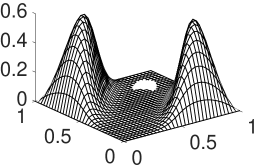
ψ(x1,x2)=10(x1x12)(x2x22)tan1[100(x1x2)6].𝜓subscript𝑥1subscript𝑥210subscript𝑥1superscriptsubscript𝑥12subscript𝑥2superscriptsubscript𝑥22superscript1100superscriptsubscript𝑥1subscript𝑥26\psi(x_{1},x_{2})=10(x_{1}-x_{1}^{2})(x_{2}-x_{2}^{2})\tan^{-1}[100(x_{1}-x_{2})^{6}].

Refer to caption

(a) ψ10subscript𝜓10\psi_{10} approximation

Refer to caption

(b) ψ11subscript𝜓11\psi_{11} approximation

Refer to caption

(c) ψ23subscript𝜓23\psi_{23} approximation

Refer to caption

(d) Analytical solution
Figure 2: Approximation of various modes compared with the analytical solution.
N=2𝑁2N=2 Number of elements
23×23superscript23superscript23~{}~{}~{}~{}2^{3}\times 2^{3} 24×24superscript24superscript24~{}~{}~{}~{}2^{4}\times 2^{4}~{} 25×25superscript25superscript25~{}~{}~{}~{}2^{5}\times 2^{5}~{} 26×26superscript26superscript26~{}~{}~{}~{}2^{6}\times 2^{6}~{} 27×27superscript27superscript27~{}~{}~{}~{}2^{7}\times 2^{7}~{}
M=1𝑀1M=1 1.77952(01)1.77952011.77952(-01) 1.75391(01)1.75391011.75391(-01) 1.72629(01)1.72629011.72629(-01) 1.72591(01)1.72591011.72591(-01) 1.72622(01)1.72622011.72622(-01)
M=3𝑀3M=3 8.85117(02)8.85117028.85117(-02) 3.72049(02)3.72049023.72049(-02) 1.08392(02)1.08392021.08392(-02) 5.66948(03)5.66948035.66948(-03) 5.07559(03)5.07559035.07559(-03)
M=5𝑀5M=5 8.90338(02)8.90338028.90338(-02) 3.66827(02)3.66827023.66827(-02) 9.31148(03)9.31148039.31148(-03) 2.35028(03)2.35028032.35028(-03) 6.04344(04)6.04344046.04344(-04)
M=7𝑀7M=7 8.90409(02)8.90409028.90409(-02) 3.66799(02)3.66799023.66799(-02) 9.30586(03)9.30586039.30586(-03) 2.34311(03)2.34311032.34311(-03) 5.93845(04)5.93845045.93845(-04)
Picard 8.90290(02)8.90290028.90290(-02) 3.66693(02)3.66693023.66693(-02) 9.29572(03)9.29572039.29572(-03) 2.33310(03)2.33310032.33310(-03) 5.83828(04)5.83828045.83828(-04)
N=4𝑁4N=4
M=1𝑀1M=1 1.77952(01)1.77952011.77952(-01) 1.75392(01)1.75392011.75392(-01) 1.72632(01)1.72632011.72632(-01) 1.72594(01)1.72594011.72594(-01) 1.72624(01)1.72624011.72624(-01)
M=3𝑀3M=3 8.84999(02)8.84999028.84999(-02) 3.71949(02)3.71949023.71949(-02) 1.08316(02)1.08316021.08316(-02) 5.66720(03)5.66720035.66720(-03) 5.07644(03)5.07644035.07644(-03)
M=5𝑀5M=5 8.90218(02)8.90218028.90218(-02) 3.66722(02)3.66722023.66722(-02) 9.30139(03)9.30139039.30139(-03) 2.34038(03)2.34038032.34038(-03) 5.94682(04)5.94682045.94682(-04)
M=7𝑀7M=7 8.90289(02)8.90289028.90289(-02) 3.66693(02)3.66693023.66693(-02) 9.29571(03)9.29571039.29571(-03) 2.33314(03)2.33314032.33314(-03) 5.83835(04)5.83835045.83835(-04)
Picard 8.90290(02)8.90290028.90290(-02) 3.66693(02)3.66693023.66693(-02) 9.29572(03)9.29572039.29572(-03) 2.33310(03)2.33310032.33310(-03) 5.83828(04)5.83828045.83828(-04)
Table 2: Relative error of series approximation for various M,N𝑀𝑁M,N and number of elements.

5.3 Test 3

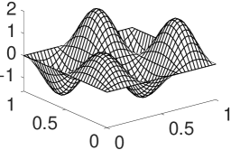
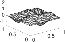
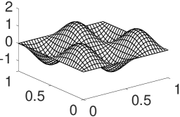
: We set a(x1,x2)=1+x12+x22,r(ψ)=exp(ψ2)+tan1ψformulae-sequence𝑎subscript𝑥1subscript𝑥21superscriptsubscript𝑥12superscriptsubscript𝑥22𝑟𝜓superscript𝜓2superscript1𝜓a(x_{1},x_{2})=1+x_{1}^{2}+x_{2}^{2},~{}r(\psi)=\exp(-\psi^{2})+\tan^{-1}\psi and seek the closed form solution ψ(x1,x2)=sin(3πx1)sin(2πx2)𝜓subscript𝑥1subscript𝑥23𝜋subscript𝑥12𝜋subscript𝑥2\psi(x_{1},x_{2})=\sin(3\pi x_{1})\sin(2\pi x_{2}). Moreover, f𝑓f is chosen accordingly with r(ψ)=ψ𝑟𝜓𝜓r(\psi)=\psi.

Refer to caption

(a) ψ00subscript𝜓00\psi_{00} approximation

Refer to caption

(b) ψ11subscript𝜓11\psi_{11} approximation

Refer to caption

(c) ψ24subscript𝜓24\psi_{24} approximation

Refer to caption

(d) Analytical solution
Figure 3: Approximation of various modes compared with the analytical solution.
N=2𝑁2N=2 Number of elements
23×23superscript23superscript23~{}~{}~{}~{}2^{3}\times 2^{3} 24×24superscript24superscript24~{}~{}~{}~{}2^{4}\times 2^{4}~{} 25×25superscript25superscript25~{}~{}~{}~{}2^{5}\times 2^{5}~{} 26×26superscript26superscript26~{}~{}~{}~{}2^{6}\times 2^{6}~{} 27×27superscript27superscript27~{}~{}~{}~{}2^{7}\times 2^{7}~{}
M=1𝑀1M=1 3.67061(01)3.67061013.67061(-01) 3.25203(01)3.25203013.25203(-01) 3.18984(01)3.18984013.18984(-01) 3.17578(01)3.17578013.17578(-01) 3.17235(01)3.17235013.17235(-01)
M=3𝑀3M=3 1.02834(02)1.02834021.02834(-02) 3.62913(02)3.62913023.62913(-02) 2.20172(02)2.20172022.20172(-02) 1.93606(02)1.93606021.93606(-02) 1.88047(02)1.88047021.88047(-02)
M=5𝑀5M=5 9.31325(02)9.31325029.31325(-02) 2.41869(02)2.41869022.41869(-02) 6.25023(03)6.25023036.25023(-03) 1.74825(03)1.74825031.74825(-03) 6.98383(04)6.98383046.98383(-04)
M=7𝑀7M=7 9.29634(02)9.29634029.29634(-02) 2.40161(02)2.40161022.40161(-02) 6.06422(03)6.06422036.06422(-03) 1.52422(03)1.52422031.52422(-03) 3.86019(04)3.86019043.86019(-04)
Picard 9.29576(02)9.29576029.29576(-02) 2.40101(02)2.40101022.40101(-02) 6.05810(03)6.05810036.05810(-03) 1.51804(03)1.51804031.51804(-03) 3.79729(04)3.79729043.79729(-04)
N=4𝑁4N=4
M=1𝑀1M=1 3.67060(01)3.67060013.67060(-01) 3.25202(01)3.25202013.25202(-01) 3.18984(01)3.18984013.18984(-01) 3.17578(01)3.17578013.17578(-01) 3.17235(01)3.17235013.17235(-01)
M=3𝑀3M=3 1.02830(02)1.02830021.02830(-02) 3.62881(02)3.62881023.62881(-02) 2.20151(02)2.20151022.20151(-02) 1.93592(02)1.93592021.93592(-02) 1.88035(02)1.88035021.88035(-02)
M=5𝑀5M=5 9.31286(02)9.31286029.31286(-02) 2.41828(02)2.41828022.41828(-02) 6.24614(03)6.24614036.24614(-03) 1.74434(03)1.74434031.74434(-03) 6.95296(04)6.95296046.95296(-04)
M=7𝑀7M=7 9.29585(02)9.29585029.29585(-02) 2.40103(02)2.40103022.40103(-02) 6.06010(03)6.06010036.06010(-03) 1.52007(03)1.52007031.52007(-03) 3.80026(04)3.80026043.80026(-04)
Picard 9.29576(02)9.29576029.29576(-02) 2.40101(02)2.40101022.40101(-02) 6.05810(03)6.05810036.05810(-03) 1.51804(03)1.51804031.51804(-03) 3.79729(04)3.79729043.79729(-04)
Table 3: Relative error of series approximation for various M,N𝑀𝑁M,N and number of elements.

6 Discussions and conclusion

The numerical results show an impressive agreement between the series approximation and the exact solutions. Since the lower order modes do not inherit sufficient spatial variability from a𝑎a, their approximations are distinguishable from the analytical solutions. Once the variability is well resolved, it takes only a few terms to obtain an accurate approximation. Moreover, the contribution of larger values of M𝑀M and N𝑁N to the overall error is insignificant as the finite element error dominates. The errors recorded show that using an excessive number of terms to construct the partial solution is obviously an overkill because the gain is insignificant compared to the computational cost. Overall, the method provides accurate approximations and the variational context provides a flexible framework to study its convergence. For the benchmark problem, the method allows the inversion of nonlinear differential operators to be achieved through a series of inversions of the discrete Laplacian. This is appealing because the nontrivial task of calculating the associated Jacobian matrix is avoided entirely. For linear reactions, the method is shown to coincide with the Picard iteration method. Even though the equivalence has not been established for a general nonlinear reaction, the numerical results of the two approaches are largely consistent.

References

  • [1] G. Adomian, A review of the decomposition method and some recent results for nonlinear equations, Mathematical and Computer Modelling, 13 (1990), pp. 17–43.
  • [2] M. Amrein and T. P. Wihler, Fully adaptive newton–galerkin methods for semilinear elliptic partial differential equations, SIAM Journal on Scientific Computing, 37 (2015), pp. A1637–A1657.
  • [3] S. Aryana, F. Furtado, V. Ginting, and P. Torsu, On series solution for second order semilinear parabolic ibvps, Journal of Computational and Applied Mathematics, 330 (2018), pp. 499–518.
  • [4] M. Badiale and E. Serra, Semilinear Elliptic Equations for Beginners: Existence Results via the Variational Approach, Springer Science & Business Media, 2010.
  • [5] N. A. Baker, D. Sept, S. Joseph, M. J. Holst, and J. A. McCammon, Electrostatics of nanosystems: application to microtubules and the ribosome, Proceedings of the National Academy of Sciences, 98 (2001), pp. 10037–10041.
  • [6] L. Boccardo and L. Orsina, Semilinear elliptic equations with singular nonlinearities, Calculus of Variations and Partial Differential Equations, 37 (2010), pp. 363–380.
  • [7] P. Bochev and R. B. Lehoucq, On the finite element solution of the pure neumann problem, SIAM review, 47 (2005), pp. 50–66.
  • [8] D. Colton and R. Kress, Inverse acoustic and electromagnetic scattering theory, vol. 93, Springer Science & Business Media, 2012.
  • [9] L. W. Gelhar, Stochastic subsurface hydrology, Prentice-Hall, 1993.
  • [10] G. Hasle, K.-A. Lie, and E. Quak, Geometric modelling, numerical simulation, and optimization, Springer, 2007.
  • [11] J.-H. He, Homotopy perturbation method for solving boundary value problems, Physics letters A, 350 (2006), pp. 87–88.
  • [12] A. Iserles, A first course in the numerical analysis of differential equations, no. 44, Cambridge university press, 2009.
  • [13] T. Kusano and S. Oharu, On entire solutions of second order semilinear elliptic equations, Journal of mathematical analysis and applications, 113 (1986), pp. 123–135.
  • [14] P.-L. Lions, On the existence of positive solutions of semilinear elliptic equations, SIAM review, 24 (1982), pp. 441–467.
  • [15] Z. Lu, D. Zhang, and B. A. Robinson, Explicit analytical solutions for one-dimensional steady state flow in layered, heterogeneous unsaturated soils under random boundary conditions, Water resources research, 43 (2007).
  • [16] P. A. Martin, Multiple scattering: interaction of time-harmonic waves with N obstacles, no. 107, Cambridge University Press, 2006.
  • [17] M. Naito et al., A note on bounded positive entire solutions of semilinear elliptic equations, Hiroshima Mathematical Journal, 14 (1984), pp. 211–214.
  • [18] W.-M. Ni, On the elliptic equation δ𝛿\deltau+ k (x) u (n+ 2)/(n- 2)= 0, its generalizations, and applications in geometry, Indiana University Mathematics Journal, 31 (1982), pp. 493–529.
  • [19] H.-G. Roos, M. Stynes, and L. Tobiska, Robust numerical methods for singularly perturbed differential equations: convection-diffusion-reaction and flow problems, vol. 24, Springer Science & Business Media, 2008.
  • [20] E. E. Rosinger, Can there be a general nonlinear pde theory for existence of solutions?, Reviews in Theoretical Science, 3 (2015), pp. 418–427.
  • [21] H. Usami, On bounded positive entire solutions of semilinear elliptic equations, Funkcial. Ekvac, 29 (1986), pp. 189–195.
  • [22] L. L. Y. Voon and M. Willatzen, Helmholtz equation in parabolic rotational coordinates: application to wave problems in quantum mechanics and acoustics, Mathematics and computers in simulation, 65 (2004), pp. 337–349.
  • [23] A.-M. Wazwaz, A comparison between adomian decomposition method and taylor series method in the series solutions, Applied Mathematics and Computation, 97 (1998), pp. 37–44.
  • [24] A. Yıldırım, He’s homotopy perturbation method for nonlinear differential-difference equations, International Journal of Computer Mathematics, 87 (2010), pp. 992–996.