GPU-based Ising Computing for Solving Balanced Min-Cut Graph Partitioning Problem

Abstract

Ising computing provides a new computing paradigm for many hard combinatorial optimization problems. Ising computing essentially tries to solve the quadratic unconstrained binary optimization problem, which is also described by the Ising spin glass model and is also the basis for so-called Quantum Annealing computers. In this work, we propose a novel General Purpose Graphics Processing Unit (GPGPU) solver for the balanced min-cut graph partitioning problem, which has many applications in the area of design automation and others. Ising model solvers for the balanced min-cut partitioning problem have been proposed in the past. However, they have rarely been demonstrated in existing quantum computers for many meaningful problem sizes. One difficulty is the fact that the balancing constraint in the balanced min-cut problem can result in a complete graph in the Ising model, which makes each local update a global update. Such global update from each GPU thread will diminish the efficiency of GPU computing, which favors many localized memory accesses for each thread. To mitigate this problem, we propose an novel Global Decoupled Ising (GDI) model and the corresponding annealing algorithm, in which the local update is still preserved to maintain the efficiency. As a result, the new Ising solver essentially eliminates the need for the fully connected graph and will use a more efficient method to track and update global balance without sacrificing cut quality. Experimental results show that the proposed Ising-based min-cut partitioning method outperforms the state of art partitioning tool, METIS, on G-set graph benchmarks in terms of partitioning quality with similar CPU/GPU times.

I Introduction

Quantum computing promises vast computational power through its massive scalability and has prompted an increasingly large landscape of emerging research areas. One of these proposed areas is that of Quantum Annealing computers [1, 2] and has been realized in the D-Wave quantum computer [3]. This paradigm of computing uses quantum interactions to find minimal energy states of a model which corresponds to the solutions of a problem. One such model is the Ising spin glass model. This model is a statistical model that describes the ferromagnetic interactions of so-called spin glasses and is explained in detail in sec. III. The ground state of the model corresponds to optimal solutions of quadratic unconstrained binary optimization problems, which many hard computational problems can be mapped to [1, 4]. However, quantum computers and quantum annealers have yet to reach maturity and the costs associated with developing and deploying one of these machines is extremely high. As a result, adapting traditional computing platforms, specifically those with highly parallel compute capabilities, to solve the Ising model has gained traction as a method of implementing and showing the practicality of quantum annealing applications.

The application areas for Quantum Annealing (QA) and the Ising model are numerous and include many hard combinatorial optimization problems such as max-flow, max-cut, graph partitioning, satisfiability, and tree based problems, which are important in many scientific and engineering areas. One particular problem area is VLSI physical design, where QA can help find optimal solutions for cell placement, wire routing, logic minimization, via minimization, and many others. The vast complexity of modern integrated circuits (ICs), some having millions or even billions of integrated devices, means that optimal solutions to these problems are almost always computationally intractable and require heuristic and analytical methods to find approximate solutions. It is well-known that traditional von Neumann based computing can not deterministically find polynomial time solutions to these hard problems [5], which shows the importance of non-traditional compute methods such as QA.

It has been shown that many hard combinatorial optimization problems can be mapped to the Ising model [4]. However, there are many challenges to handle practical problems using the Ising model. For instance, for the balanced min-cut partitioning problem, the balance constraint will lead to a complete graph in the resulting Ising model. The reason is that the balance constraint is a global constraint. As a result, each Ising spin glass is connected to all the Ising spins glasses in the graph, therefore; each local spin update becomes a global update. Current Ising model solvers and quantum annealing computers often do not have architectures amenable to the embedding of problems with complete graphs, e.g., the Chimera graph architecture used in D-wave computer [3]. However, recent study shows that balanced min-cut problems on the D-wave computer indeed yields better results than the state of the art partitioning solvers like METIS [6], but the problem sizes solved are still limited to thousands of nodes and requires co-processing on traditional hardware due to the limited number of available qubits in the QA machine.

In this work, we apply Ising computing to solve a more practical combinatorial problem – the balanced min-cut graph partitioning problem. We will first outline the Ising model and how a practical problem like the balanced min-cut partitioning problem can be mapped to it. We have the following contributions:

• We will first present a standard implementation of the Ising annealing solution for 2-way balanced graph partitioning problem on the GPU platform. Due to the global balance constraint, it will lead to a complete graph in the Ising model, which requires each spin glass to perform a global update. Such global update from each spin glass will diminish the efficiency of GPU computing, which favors many localized memory accesses for each thread.

• To mitigate complete graph problem, we propose an novel balance-constraint efficient globally decoupled Ising (GDI) model and the corresponding annealing algorithm, in which the local update is still preserved to maintain the efficiency. As a result, the new Ising solver essentially eliminates the need for the fully connected graph and will use a more efficient method to track and update global balance without sacrificing cut quality. The proposed methods will utilize an asynchronous update schemes to ensure uncorrelated spin updates and, in conjunction with decaying random flips, will naturally add energy to the model that will help to escape local minima in the solution.

• We show that the proposed 2-way min-cut graph partitioning Ising solver produces cut results that compete favorably with the state of the art graph partitioning software METIS [7], a heuristic with close to linear time complexity. Our numerical results on the published G-set benchmarks further show that the proposed Ising solver method will vastly decrease computation time compared to the standard method, will achieve better cut results (lower cut values and perfectly balanced partitions) than METIS on many large graph problems, and will find these solution in a comparable time to METIS.

This article is organized as follows. Section II reviews some related works for quantum computing and other recently proposed hardware based Ising machines. Section III reviews the basic concepts of Ising models and the annealing method for Ising models. Section IV proposes two Ising solvers for the balanced min-cut graph partitioning problem. The graph partitioning results and comparison against METIS and discussions are presented in Section VI. At last, Section VII concludes this article.

II Background and related work

While quantum computing has yet to reach maturity, there exists a number of other hardware-based Ising model solvers which have been proposed to exploit the highly parallel nature of this model. On the other hand, the adiabatic process is not just limited to the quantum devices and systems. Such natural adiabatic computing can be found in many devices and systems. The so-called natural computing maps the problems to natural phenomena characterized by intrinsic convergence properties. In [8], a novel CMOS based annealing solver was proposed in which an SRAM cell is used to represent each spin and thermal annealing process was emulated to find the ground state. In [9, 10], the FPGA-based Ising computing solver has been proposed to implement the simulated annealing process. However, these hardware Ising based solvers suffer from several problems. First, the Ising model for many practical problems can lead to very large connections among Ising spins or cells. Furthermore, embedding those connections into the 2-dimensional fixed degree spin arrays in VLSI chips is not a trivial problem and requires mitigation techniques such as cell cloning and splitting as proposed in [9, 10]. Second, ASIC implementations are not flexible and can only handle a specific problem and FPGA implementations require architectural redesign for different problems. Third, one has to design hardware for the random number generator for each spin cell and simulate the temperature changes, which has significant chip area costs which resulting in scalability degradation. An optical parametric oscillator based Ising machine was recently proposed [11] in which the annealing is carried out by interaction of laser pulses in the optical fibers. Also electronic Oscillator-based Ising machine implemented by using CMOS electronic circuits was demonstrated on max-cut problems [12]. Again this work can only solve very small and simple problems as it uses discrete electronic components.

Based on the above observations and the highly parallel nature of the Ising model, in this work, we propose using the General Purpose Graphics Processing Unit (GPGPU or, more simply GPU) as the Ising model annealing computing platform. The GPU is a general computing platform, which can provide much more flexibility over VLSI hardware based annealing solutions as a GPU can be programmed in a more general way, enabling it to handle any problem that can be mapped to the Ising model. The GPU is an architecture that utilizes large amounts of compute cores to achieve high throughput performance. This allows for very good performance when computing algorithms that are amenable to parallel computation while also having very large data sets which can occupy the computational resources of the GPU [13, 14]. Previous Ising model solvers on GPUs have been proposed already [15, 16, 17]. However, they still focus on small physics problems which assume a nearest neighbor model only. Their models, are amenable to the GPU computing as it is easily load balanced across threads but is not general enough to handle practical combinatorial optimization problems in EDA and other fields. Furthermore, many GPU-based methods use a checkerboard update scheme, but this is still only practical for the nearest neighbor model without using complicated graph embedding.

Recently the GPU-based Ising computing solution was proposed for solving the max-cut combinatorial problem [18]. The resulting Ising solver show many orders of magnitude speedup over IBM CPLEX mathematical programming solver [19] while with even better cut results. At the same time, the Ising max-cut solver has $2000\times$ speed-up over CPU-based Ising solver for many large cases. However, the max-cut problem has a simple mapping to the Ising model and more difficult problems with more complicated constraints are yet to be explored to show that the GPU-based Ising computing can be used for many practical combinatorial optimization problems.

III Ising model and Ising computing

III-A Ising model overview

The Ising model is a mathematical model of the ferromagnetic interactions between so-called “spin glasses” or just “spins” inside of a two dimensional lattice. In this model, each spin is connected to neighbors by weighted edges and the model itself is affected by some external magnetic force or bias and is depicted in Fig. 1. Finding the minimal energy state of this model, known as the ground state, is an NP-hard problem [20]. However, the nature of this model makes finding the ground state through heuristic methods highly amenable to fine grained parallelism. Thus it is highly desirable to map other computationally intractable problems to the problem of finding minimal energy states of the Ising model.

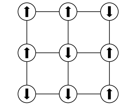
Figure 1: The 2D nearest neighbor Ising model.

The value of each spin $\sigma_{i}$ can be discrete values of $1$ or $-1$, i.e., $\sigma_{i}\in\{-1,1\}$. The energy of the model, or the Hamiltonian, can be defined by (1):

$$\mathcal{H}_{i}(\sigma_{i})=-\sum\limits_{j}J_{i,j}\sigma_{i}\sigma_{j}-h_{i}\sigma_{i}$$ (1)

In the preceding equation $J_{i,j}$ is the interaction weight between a spin $\sigma_{i}$ and its neighbor $\sigma_{j}$ while $h_{i}$ describes the external force acting on the spin glass.

To determine the spin value of a glass $\sigma_{i}$, we can find its local energy $\mathcal{H}_{(}sigma_{i})$. To do this, we rewrite (1) as:

$$\mathcal{H}_{i}(\sigma_{i})=\left(-\sum\limits_{j}J_{i,j}\sigma_{j}-h_{i}\right)\sigma_{i}=-S\times\sigma_{i}$$ (2)

We can see from (2) that the spin value of a glass can actually be determined from the sign of $S$, e.g., if $S>0$ then $\sigma_{i}=1$, else if $S<0$ then $\sigma_{i}=-1$ and if $S=0$ we allow the spin value to be random. This process describes the local spin update. We note that every spin glass only requires knowledge of connected neighbors to minimize its own local energy. The only restriction on this is that the updates for each individual spin must not be correlated. If this is satisfied, then each spin can be updated independently and in parallel [8, 9, 10, 15, 16]. Then the global energy of the whole Ising model is given by the following (3),

$$\mathcal{H}(\sigma_{1},\sigma_{2},...,\sigma_{n})=-\sum\limits_{\langle i,j\rangle}J_{i,j}\sigma_{i}\sigma_{j}-\sum\limits_{i}h_{i}\sigma_{i}$$ (3)

In this equation, $\langle i,j\rangle$ refers to every combination of spin glass interactions. This means that minimizing the local energy of each spin glass will lead to the minimum global energy as well. Finding this ground state is equivalent to solving an unconstrained Boolean optimization problem[21]. This is useful since it has been shown that many intractable problems can be mapped to this model [4].

Previous implementation methods that solve the Ising model rely on the use of the nearest neighbor model as shown in Fig. 1. However, this requires the use of graph embedding, which is an NP-hard problem, to successfully map practical problems to the Ising model [9]. This practice is required for other solution methods using ASIC and FPGA implementations which are less flexible. In contrast, our use of the GPGPU allows us to directly use a generally connected Ising model, as shown in Fig. 2, to easily accommodate complex problem cases.

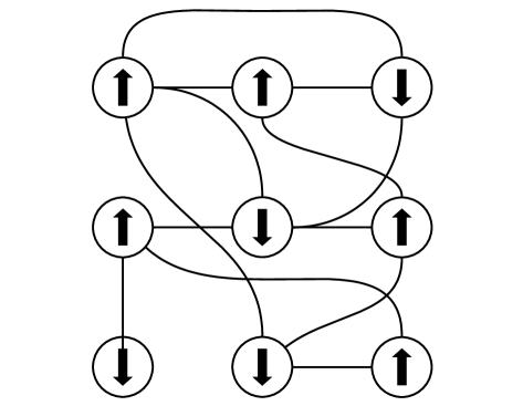
Figure 2: An example of a generally connected Ising model.

III-B Annealing method for Ising model solution

A trivial solution approach to solving the Ising model would be to utilize the classical thermal annealing approach, Simulated Annealing (SA) [22]. This method simulated the thermal annealing process by creating a high “temperature” environment that allows the heuristic to escape local minima during the search for the minimum global energy state as depicted in Fig. 3. As the heuristic runs, the temperature is gradually decreased allowing it to settle on a final solution state. While this may be a viable method to solve the Ising model, it requires sequential updates and global energy calculations at every step, which is costly, and unnecessary for the standard Ising model.

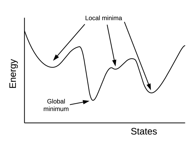
Figure 3: Depiction of the local minima and global minimum in the energy minimization problem.

To find the ground state of the Ising model in this work, we utilized a modified annealing algorithm that better mimics a QA computer and also avoids the global energy calculation as shown in Algorithm 1. This algorithm has the added benefit of allowing us to exploit the parallelism in the local spin glass updates, which we will introduce in a later section, while also allowing us to avoid local minima. The algorithm allows each spin glass to update by independently minimizing its own local energy without considering global energy. Furthermore, to avoid the local minima, spin glasses are randomly flipped with a gradually decaying probability, e.g., each spin has a $50\%$ probability to flip at the start of simulation, this probability will exponentially decrease during simulation.

Algorithm 1 Modified Ising annealing algorithm

1:  input: ($M$, $N$, ${\bf S}$)

2:  initialize all $\sigma_{i}$ in ${\bf S}$

3:  for sweep-id in {1, 2, …, $M$} do

4:     for $\sigma_{i}$ in ${\bf S}$ do

5:        $\sigma_{i}\leftarrow\mathrm{argmin}(H(\sigma_{i}))$ based on (2)

6:     end for

7:     randomly choose and flip $N$ spin glasses in ${\bf S}$

8:     decrease $N$

9:  end for

In this algorithm we have three parameters: $M$ which is the number of update “sweeps”, $N$ which controls the spin glasses to randomly flip, and $S$ which is the set of all spin glasses $\sigma_{i}$ in our model. We start by initializing all of our spin glasses $\sigma_{i}$ in our model(graph) $S$. Then, $M$ sweeps are calculated. During each sweep, every spin glass will chose its spin value $\sigma_{i}\in\{1,-1\}$ such that its local energy is minimized according to its interactions with its neighbors. At the end of an update sweep, $N$ spin glasses are randomly flipped and $N$ decays according to a desired decay schedule such as an exponential decay. This process is repeated $M$ times. During this process, as each spin glass minimizes its local energy, the global energy will also decrease. The random flips are introduced at each phase to avoid local energy minima and are decayed to allow the states to settle at the end of the simulation.

We want emphasize that this Ising annealing process is fundamentally different from the traditional simulated annealing process [22], in which we have to measure or compute the global cost function for each move and make the statistical decision (accept or rejection), which is affected by the temperature. For Ising annealing, all the moves are local as shown in step 5 in Algorithm 1. As a result, steps 3 to 7 can be done in parallel for all the cells, which indicates the massive fine-grained parallelism, which in general is not possible in traditional simulated annealing process. The only restriction on this parallelism is that spin updates cannot be correlated [23].

IV Ising model for balanced min-cut partitioning

In previous works, the Ising model has been used to solve the max-cut problem [8, 9, 10, 18], but as pointed out in [4], many other NP-complete and NP-hard problems can be mapped to this model as well. The choice to use max-cut in these other works stemmed from the fact that it is trivial to map to the Ising model, making it ideal as a proof of concept problem. However, very little work has been done to map and solve other, more practical problems.

For this reason, this article will show that the balance min-cut graph partitioning problem (min-cut) can be successfully mapped to the Ising model and solved with solution quality rivaling that of state of the art partitioners such as the METIS solver [7]. This problem is highly practical as partitioning is a key algorithm in a wide variety of applications such as VLSI Physical Design.

IV-A Min-cut Hamiltonian

To formulate the Hamiltonian for the min-cut problem, we must first define min-cut. Given a graph $G(V,E)$, with edge set $E$ and vertex set $V$, partition $G$ into two subsets ($V_{1},V_{2}$) such that the edges between $V_{1}$ and $V_{2}$ are minimized and that $|V_{1}|=|V_{2}|$. In other words, we want to assign each vertex in the graph to one of two sets such that we minimize the connections between the two sets while also keeping the size of each set equal. Unfortunately, this problem has been shown to be NP-hard [24].

To facilitate the formulation of the Hamiltonian and subsequent mapping to the Ising model, we need to modify certain constraints so that we can put the problem in a form that is amenable to unconstrained binary optimization. To do this, we will define our Hamiltonian to be the summation of two separate Hamiltonian functions, $\mathcal{H}_{A}$ and $\mathcal{H}_{B}$. Minimizing the energy of this Hamiltonian will be equivalent to solving the min-cut problem. Furthermore, we will relax the constraint that $|V_{1}|=|V_{2}|$ and allow some minor imbalance between each set (which we will now call partitions). Lastly, we will define the spins in our Ising model to be the indication of which partition a spin glass belongs in, i.e., if $\sigma_{i}=1$ then $\sigma_{i}\in V_{1}$ and if $\sigma_{i}=-1$, then $sigma_{i}\in V_{2}$.

$$\centering\mathcal{H}_{cut}=\mathcal{H}_{cut,A}+\mathcal{H}_{cut,B}\@add@centering$$ (4)

The first Hamiltonian $\mathcal{H}_{cut,A}$ is a penalty function that adds energy to our system in (4) when the partition sizes are not equal and is defined as:

$$\centering\mathcal{H}_{cut,A}=A((\sum\limits_{i}\sigma_{i})^{2})\@add@centering$$ (5)

Recall that $\sigma_{i}\in{-1,1}$, then we can see from (5) that it will equal zero (be minimized) when there are an equal number of negative and positive spins. Otherwise, this Hamiltonian will evaluate to a positive number and add energy to the system. The constant $A$ is a parameter that can be tuned to affect the weight of the penalty incurred from imbalance.

The Hamiltonian $\mathcal{H}_{cut,B}$ is responsible for partitioning the spin glasses such that the edges between the partitions are minimized and is defined as:

$$\centering\mathcal{H}_{cut,B}=B(\sum\limits_{\langle i,j\rangle}\frac{1-\sigma_{i}\sigma_{j}}{2})\@add@centering$$ (6)

In (6) we can see that when $\sigma_{i}=\sigma_{j}$ the energy is minimal and the effect is opposite when this is not the case. Effectively, this means that each vertex will produce the least amount of energy when it is placed in the same partition that the majority of its neighbors occupy. The parameter $B$ can be tuned to increase or decrease the penalty of this Hamiltonian.

In general, when choosing the value of $A$ and $B$, the following rule, as outlined in [4], can be applied:

$$\centering\frac{A}{B}\geq\frac{min(2\Delta,N)}{8}\@add@centering$$ (7)

In this equation, $\Delta$ is the maximum degree of the graph $G$ and $N$ is the number of spins used to encode the problem, which for our implementation is just the number of vertices in $G$.

By minimizing the energy of (4), we can obtain a balanced partitioning of a graph problem while also achieving minimized cuts between the partitions. Unlike the traditional Ising model, this Hamiltonian contains two sub-Hamiltonians. Furthermore, we also must note that the Hamiltonian in (5) requires that each spin-glass have knowledge of every spin glass in the model. This effectively produces a fully connected graph and vastly increases the complexity of the problem, which will be addressed in the following sections.

V GPU-based Ising solver for balanced min-cut problem

V-A GPU architecture

The general purpose GPU is an architecture designed for highly parallel workloads which is leveraged by Nvidia’s CUDA, Compute Unified Device Architecture, programming model [13]. The Nvidia GPU architecture is comprised of several Symmetric Multiprocessors (SMs), each containing a number of “CUDA” cores, and a very large amount of DRAM global memory [14]. The Kepler architecture based Tesla K40c GPU, for example, has 15 SMs for a total of 2880 CUDA cores (192 cores per SM), and 12GB DRAM global memory. Additionally, each SM has additional special function units, shared memory, and cache. Compared to a multi-core CPU, the GPU offers much more parallel computational resources at the expense of higher latency. That is, it can do more at the same time but each operation takes longer compared to the CPU. In general, as long as the data set can occupy the large resources of the GPU and each operation being performed in parallel is not latency constrained, the GPU will see significant performance gains over the CPU.

The CUDA programming model, shown in Fig. 4, extends the C language adding support for thread and memory allocation and also the essential functions for driving the GPU [25]. The model makes a distinction between the host and device or the CPU and GPU respectively. The model uses an offloading methodology in which the host can launch a device kernel (the actual GPU program) and also prepare the device for the coming computation, e.g.,the host will create the thread organization, allocate memory, and copy data to the device. In practice, a programmer must call many threads which will be used to execute the GPU kernel. Thread organization is therefore extremely important in GPU programming. Threads are organized into blocks which are organized into grids. Each block of threads also has its own shared memory which is accessible to all the threads in that block. Additionally, the threads in the block can also access a global memory on the GPU which is available to all threads across all blocks.

Figure 4: The Nvidia CUDA programming model

The GPU fundamentally focuses on throughput over speed. This throughput is achieved through the massive compute resources able to be run in parallel. Because of this, it is important to realize that the GPU is not meant for small data sets or extremely complicated operations that may be better suited for a powerful, low latency, CPU. Instead, the GPU is meant to execute relatively simple instructions on massive data in parallel that can occupy the GPU resources for an extended period of time.

V-B Standard implementation

To first validate the GPU implementation of the Ising model solver for the min-cut problem, we construct a parallel algorithm from the one shown in Algorithm 1 but with the modified Hamiltonians for the min-cut problem.

As mentioned before, spin glass updates can be performed in parallel during a sweep. However, the restriction on this is that the updates must be performed independently. Furthermore, the updates of spins must happen asynchronously to avoid biphasic oscillation. Fortunately, this can be accomplished in the GPU simply by allowing race conditions on read operations. Effectively, this just means that when a spin calculates its own local energy, it will use the current energy of its neighbors which may, or may not, have already minimized their own local energy. To facilitate this, the following algorithm for the GPU implementation has been used:

Algorithm 2 Standard implementation for GPU Ising model annealing for balanced min-cut problem

   input: ($M$, $P_{f},{\bf S}$)

  initialize ALL $\sigma_{i}$ in ${\bf S}$

  for sweep-id in {1, 2, …, $M$ do

     for all $\sigma_{i}\in\bf S$ in parallel do

        $\sigma_{i}\leftarrow\mathrm{argmin}(\mathcal{H}_{cut,A}(\sigma_{i})+\mathcal{H}_{cut,B}(\sigma_{i}))$

        flip $\sigma_{i}$ with probability $P_{f}$

     end for

     reduce $P_{f}$

  end for

In this algorithm the spins for each glass are initialized and $M$ update sweeps are performed. During each sweep, every spin glass, in parallel, chooses the value of $\sigma_{i}$ that minimizes the Hamiltonian in (4). In effect, this means each spin will read the spin values of all of its connected neighbors (to evaluate (6)) as well as the spin values of all spins in the entire graph (to evaluate (5)). After a spin glass finishes its update, it will randomly flip with a probability determined by $P_{f}$. Once every spin has updated and decided to flip or not, the flip probability $P_{f}$ is reduced according to a cooling schedule. This process is then repeated.

The flip probability $P_{f}$ is initially determined by the number of nodes that should be randomly flipped, which we will call $N_{rf}$. That is, if there are $500$ nodes, and the $N_{rf}$ is $100$, then $P_{f}$ will initially be calculated to be $0.20$. When deciding to flip or not, each spin generates a uniformly distributed random number between $0.00$ and $1.00$. If this number is higher than $P_{f}$ then the spin will not flip, however, if it is equal or lower, then it will.

Practically, each spin is handled by a single thread in the GPU. If the number of spin glasses exceeds the number of threads available, then threads will be assigned multiple spin glasses to update. For the random number generation, the CUDA cuRAND library is used which allows for efficient random number generation in parallel. We also note, as mentioned previously, that each spin update should not be correlated. For this reason, updates are done asynchronously. In effect, this means that a spin glass will check the status of its neighbor spins during an update but it will not be guaranteed that its neighbors have not already finished their own update operation.

V-C Globally Decoupled Ising implementation

While Algorithm 2 does successfully calculate a balanced min-cut partition, as we will show in the results section, it is also heavily constrained by the direct computation of $\mathcal{H}_{cut,A}$ as shown in (5). This means that for each spin glass in the model, it must traverse the entire model to assess the status of every spin glass and determine the balancing penalty. This is obviously a heavy computational step and will drastically limit the performance of the algorithm as the problem size increases. This is actually is one of major challenges for Ising based computing as many constraints will lead to dense or complete Ising graphs.

One of the major contributions of this work is to find a way to mitigate this challenging problem. To mitigate this problem, we have to find a better way to deal with the balance constraints instead of using the standard Ising model. In this way, we still keep the spin updates local (each spin glass no longer has to traverse the entire model), which is critical to maintaining the efficiency and scalability for the GPU-based computing, while making the global connections decoupled. Therefore, we propose to use a Globally Decoupled Ising (GDI) solver.

Algorithm 3 Globally Decoupled Ising (GDI) implementation for GPU Ising model annealing for balanced min-cut problem

   input: ($M$, $P_{f},{\bf S}$)

  initialize ALL $\sigma_{i}$ in ${\bf S}$

  $G=\sum\limits_{i}\sigma_{i}$

  for sweep-id in {1, 2, …, $M$ do

     for all $\sigma_{i}\in\bf S$ in parallel do

        $\sigma_{i}\leftarrow\mathrm{argmin}(\mathcal{H}_{cut,B}(\sigma_{i})+A(G+\sigma_{i})^{2})$

        $G=\mathrm{atomicAdd}(G+\sigma_{i})$

        flip $\sigma_{i}$ with probability $P_{f}$

     end for

     reduce $P_{f}$

  end for

Specifically, in Algorithm 3, we pre-compute the global balance before starting the first update sweep and store this value in a global variable $G$. Then, as each thread performs its update during a sweep, it uses this value to determine the balancing penalty it’s spin glass may incur. After deciding which partition will minimize the spin glass local energy, the thread updates the $G$ value so that all other spins glasses have knowledge of the new balance. It should be noted that because this is happening in parallel, the balance that some threads see may not be the actual balance when that thread updates the spin glass it is responsible for. Furthermore, an atomic addition is used to update $G$ which will incur some computational penalty (but at much less cost than the method in Algorithm 2). This atomic operation ensures the validity and integrity of the $G$ value at the end of each sweep as it eliminates “data race” between threads updating this value.

V-D Further discussion and comparison

The primary difference in the two algorithms is the modification to the calculation of the balancing Hamiltonian. The major effect is that we no longer require each node to traverse the entire graph at each update step to calculate the global balance. Rather, the global balance is pre-computed and then individually read, while modified (through atomic operations) by one node at a time.

With respect to implementation, we notice that the standard version requires a higher random flip probability than the enhanced version to achieve good cut results. The reason for this is that the enhanced version naturally introduces more noise, or randomness, to the update scheme while the standard version is more constrained by the global update. That is, it is less willing to violate the global constraint as each node has nearly perfect knowledge of the state of the global balance. For this reason, during implementation, we typically need a $5X$ increase to the value of $P_{f}$ when using the standard implementation.

VI Experimental results and discussions

In this section, we present the experimental results showing the quality of our parallel GPU-based Simulated Quantum Annealing solver for the balanced min-cut problem. The CPU-based solution is done using a Linux server with 2 Xeon processors, each having 8 cores (2 threads per core) and a total of 32 threads, and 72 GB of memory. On the same server, we also implement the GPU-based solver using the Nvidia Tesla K40c GPU which has 2880 CUDA cores and 12 GB of memory. Test problems from the G-set benchmark [26] are used for testing.

TABLE I: Summary of results for the standard (std.) and Globally decoupled (GDI) Ising solver compared with the METIS results. Graphs with less than 1000 nodes are omitted

Graph-ID	# nodes	# edges	Density	$t_{\text{Metis}}$	$t_{\text{Ising,GDI}}$	$t_{\text{Ising,std.}}$	$cut_{\text{Metis}}$	$cut_{\text{Ising,GDI}}$	$cut_{\text{Ising,std}}$	$bal_{\text{Metis}}$	$bal_{\text{Ising,GDI}}$	$bal_{\text{Ising,std.}}$
G70	10000	9999	2.0E-4	1.6E-2	0.34929	31.88844	487	507	555	5	0	0
G81	20000	40000	2.0001E-4	1.6E-2	0.15046	22.40281	210	240	242	5	0	0
G77	14000	28000	2.8573E-4	1.2E-2	0.15686	15.67784	220	212	232	3	0	0
G67	10000	20000	4.0004E-4	0.08	0.15579	11.20150	216	216	244	1	0	0
G72	10000	20000	4.0004E-4	0.08	0.15707	11.23208	216	212	230	1	0	0
G66	9000	18000	4.4449E-4	8.0E-3	0.15810	10.08537	196	220	242	2	0	0
G65	8000	16000	5.0006E-4	8.0E-3	0.15766	9.01416	178	168	178	3	0	0
G62	7000	14000	5.7151E-4	8.0E-3	0.15730	7.87871	144	146	148	1	0	0
G60	7000	17148	7.0002E-4	2.8E-2	0.21494	9.31080	3330	3115	3321	2	0	0
G57	5000	10000	8.0016E-4	4.0E-3	0.15679	5.64559	140	110	252	0	0	0
G55	5000	12498	1.0001E-3	0.02	0.21558	6.45212	2463	2308	2391	0	0	0
G48	3000	6000	1.33378E-3	4.0E-3	0.15601	3.45138	120	124	194	1	0	0
G49	3000	6000	1.33378E-3	4.0E-3	0.15632	3.45322	74	60	136	0	0	0
G50	3000	6000	1.33378E-3	0	0.15617	3.45544	58	50	92	1	0	0
G64	7000	41459	1.6924E-3	3.2E-2	0.38691	5.89811	9946	9787	9967	2	2	0
G32	2000	4000	2.001E-3	0	0.12023	2.30673	50	40	54	1	0	0
G33	2000	4000	2.001E-3	0	0.12019	2.30543	54	50	78	1	0	0
G34	2000	4000	2.001E-3	0	0.12044	2.31117	112	86	150	1	0	0
G58	5000	29570	2.366E-3	2.4E-2	0.34457	3.98248	7226	6921	7302	1	0	0
G36	2000	11766	5.8859E-3	8.0E-3	0.23601	1.63955	2896	2722	2898	0	0	0
G35	2000	11778	5.8919E-3	1.2E-2	0.20426	1.77944	2942	2771	2841	1	0	0
G38	2000	11779	5.8924E-3	1.2E-2	0.26296	1.63863	2866	2688	2801	1	0	0
G37	2000	11785	5.8954E-3	1.2E-2	0.24608	1.63948	2921	2781	2834	1	0	0
G22	2000	19990	0.01	1.2E-2	0.15961	0.87029	6925	6739	6803	0	0	0
G23	2000	19990	0.01	1.6E-2	0.15989	0.86660	6946	6702	6743	0	0	0
G24	2000	19990	0.01	1.6E-2	0.16047	0.96611	7022	6719	6809	1	0	0
G28	2000	19990	0.01	1.2E-2	0.16016	0.86641	6961	6753	6781	0	0	0
G30	2000	19990	0.01	1.6E-2	0.16170	0.86767	6978	6702	6774	1	0	0
G31	2000	19990	0.01	1.2E-2	0.16086	1.00123	6957	6683	6798	1	0	0
G51	1000	5909	1.183E-2	4.0E-3	0.18105	0.92766	1513	1383	1458	0	0	0
G53	1000	5914	1.184E-2	4.0E-3	0.19386	0.92421	1498	1366	1368	0	0	0
G52	1000	5916	1.1844E-2	4.0E-3	0.19584	0.92683	1446	1394	1399	0	0	0
G54	1000	5916	1.1844E-2	4.0E-3	0.20007	0.92612	1465	1356	1430	0	0	0
G43	1000	9990	0.02	8.0E-3	0.15092	0.51411	3542	3350	3382	0	0	0
G44	1000	9990	0.02	8.0E-3	0.15365	0.51538	3565	3361	3402	0	0	0
G45	1000	9990	0.02	8.0E-3	0.15322	0.51169	3522	3347	3397	0	0	0
G46	1000	9990	0.02	4.0E-3	0.15210	0.51384	3573	3353	3386	0	0	0
G47	1000	9990	0.02	8.0E-3	0.15191	0.51398	3520	3350	3396	0	0	0

VI-A Solution time study

We firstly investigate the performance of the standard Ising solver and the globally decoupled method developed in the paper, followed by discussion of its performance compared to the state of the art partitioning software.

The direct Ising solver implementation of the min-cut partitioning problem leads to a complete graph requiring a global update for each spin glass in the model. In other words, when each node updates during an annealing sweep, it must visit every other node in the graph. To address this, we proposed the balance constraint efficient annealing algorithm in 3. In the GDI version, we mitigate the issue of global update by utilizing a global variable to store the balance of the graph partition which is updated using atomic operations by each node. This means each node only needs to perform a single read and atomic add operation on this variable.

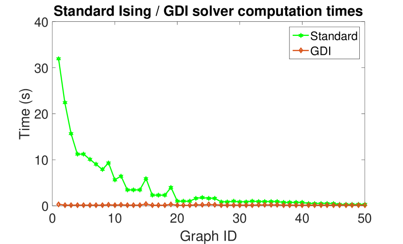
Figure 5: Performance gains of the GDI solver min-cut algorithm.

In Fig 5, the graph problems solved are sorted from lowest to highest density where density is calculated as $density=(2\times\#edges)/(\#nodes\times(\#nodes-1))$ . The nature of the G-set graphs used are such that low density graphs have many more nodes and edges than the high density graphs. For this reason, the graph can be looked at as being sorted from large complexity to smallest complexity. As we can see, the direct implementation quickly increases in computation time as the problem become more and more complex. Comparatively, the GDI version appears constant in these results as the computations times are not comparable.

We further show the performance results of the GDI solver algorithm and the performance of METIS, widely considered the gold standard for partitioning software.

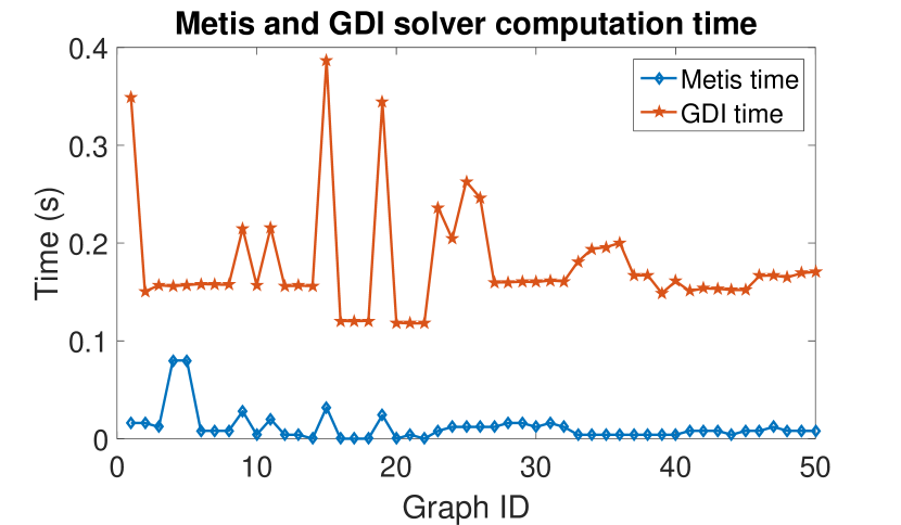
Figure 6: Performance comparison of the GDI GPU Ising solver and METIS.

We can see from Fig. 6 that, while METIS is still able to beat the proposed solver in terms of speed, the proposed Ising solver is quite close and comparable in time with all solutions taking less than a second, even for the larger graphs.

VI-B Solution quality study

To study the solution quality of the proposed method, wee first show that the solution quality of the direct implementation of the GPU-based Ising solver and the GDI solver are similar.

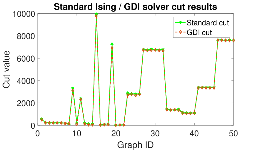
Figure 7: Solution quality of the proposed GPU-based Ising solvers.

As seen from Fig. 7 the solution quality of the GDI method not only achieves similar solution results, it also consistently achieves cut values marginally lower than the standard implementation.

To measure the solution quality produced by the proposed method, we compare balanced min-cut partitioning results of the proposed method with the results produced by METIS. We omit the solution quality results of the direct implementation as they are similar to the GDI method proposed. For fairest comparison, we ensured both METIS and the GPU-based Ising solver used a highly constrained balance criteria. For each graph, we run both solvers 10 times and use the best solution quality found. The quality is measured by comparing the cut values of the solvers. Cut values are defined as the number of edges that connect one partition to the other.

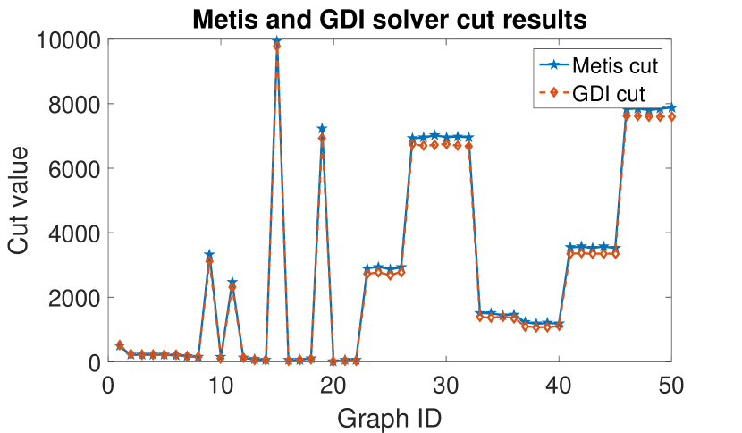
Figure 8: Cut quality results for the G-set benchmark problems.

As seen from Fig. 8, the proposed Ising solver GPU method achieves the same or better quality results for almost every graph tested. Of the 51 graphs, the Ising solver method achieved worse quality in only 5 graphs and produced the exact same quality in 1 graph. Even then, the Ising solver results were very close to METIS. We note that the all of the graphs where Ising solver achieved worse quality were very sparse graphs, i.e., their graph density was very low, which suggests that utilization of the Ising model can be difficult for these types of graphs.

While the balancing constraint on METIS was set to be as restrictive as possible, $22$ of the the $51$ graphs tested had imbalanced partitions. In contrast, the proposed GDI solver achieved perfect balance for all but one graph tested. We also remark that the balances achieved by METIS were still quite good with the worst imbalance being only 5 nodes.

These results, as summarized in Table I, show that the proposed method is able to achieve better solution quality than the state of the art METIS solver, both in terms of balanced partitions and minimized cut values. Furthermore, even for large and dense graphs, the proposed solver finished in a time comparable to METIS.

VII Conclusion

In this work, we have proposed a GPU-based Ising spin glass model solver applied to the balanced min-cut graph partitioning problem. The work presented the Ising spin glass model and the annealing solution method for solving Unconstrained Quadratic Binary Optimization problems while additionally showing the method for mapping the min-cut problem to this model. A standard GPU implementation is presented in addition to a Globally Decoupled Ising annealing algorithm which mitigates the costly global updates during each annealing sweep. Numerical results show that both the standard and enhanced annealing algorithms achieve high quality, and nearly perfectly balanced, partitioning results that compete with and exceed the partitioning quality achieved by the state of the art partitioning solver, METIS. Furthermore, the proposed GDI method can produce results much faster than the standard method, resulting in computation times comparable to the METIS solver. Experimental results show that the proposed Ising-based min-cut partitioning method outperforms the state of art partitioning tool, METIS, on G-set graph benchmark in terms of partitioning quality with similar CPU/GPU times.

References

- [1] M. W. Johnson, M. H. S. Amin, S. Gildert, T. Lanting, F. Hamze, N. Dickson, R. Harris, A. J. Berkley, J. Johansson, P. Bunyk, E. M. Chapple, C. Enderud, J. P. H. an K. Karimi, E. Ladizinsky, N. Ladizinsky, T. Oh, I. Perminov, C. Rich, M. C. Thom, E. Tolkacheva, C. J. S. Truncik, J. W. S. Uchaikin, B. Wilson, and G. Rose, “Quantum annealing with manufactured spins,” Nature, vol. 473, pp. 194 EP–, 2011.
- [2] S. Boixo, F. F. Ronnow, S. V. Isakov, Z. Wang, D. Wecker, D. A. Lidar, J. M. Martinis, and M. Troyer, “Evidence for quantum annealing with more than one hundred quibits,” Nature Physics, 2014.
- [3] “D-Wave Computer,” 2018. http://www.dwavesys.com.
- [4] A. Lucas, “Ising formulations of many np problems,” Frontiers in Physics, vol. 2, p. 5, 2014.
- [5] C. Papadimitriou and K. Steiglitz, Combinatorial Optimization: Algorithms and Complexity. Dover Publications, 1998.
- [6] H. Ushijima-Mwesigwa, C. F. A. Negre, and S. M. Mniszewski, “Graph partitioning using quantum annealing on the d-wave system,” in Proceedings of the Second International Workshop on Post Moores Era Supercomputing, PMES’17, (New York, NY, USA), pp. 22–29, ACM, 2017.
- [7] G. Karypis and V. Kumar, “A fast high quality multilevel scheme for partitioning irregular graphs,” SIAM Journal on Scientific Computing, vol. 20, no. 1, pp. 359–392, 1999.
- [8] M. Yamaoka, C. Yoshimura, M. Hayashi, T. Okuyama, H. Aoki, and H. Mizuno, “A 20k-spin ising chip to solve combinatorial optimization problems with cmos annealing,” IEEE Journal of Solid-State Circuits, vol. 51, pp. 303–309, Jan 2016.
- [9] H. Gyoten, M. Hiromoto, and T. Sato, “Area efficient annealing processor for ising model without random number generator,” IEICE Trans. on Fundamentals of Electronics, Communications and Computer Science(IEICE), vol. E101.D, pp. 314–323, 2018.
- [10] C. Yoshimura, M. Hayashi, T. Okuyama, and M. Yamaoka, “Implementation and evaluation of fpga-based annealing processor for ising model by use of resource sharing,” Internation Journal of Networking and Computing, vol. 7, 2017.
- [11] P. McMahon, “To solve optimization problems, just add lasers: An odd device known as an optical ising machine could untangle tricky logistics,” IEEE Spectrum, vol. 55, pp. 42–47, Dec 2018.
- [12] T. Wang, L. Wu, and J. Roychowdhury, “New computational results and hardware prototypes for oscillator-based ising machines,” in Proceedings of the 56th Annual Design Automation Conference 2019, DAC ’19, (New York, NY, USA), pp. 239:1–239:2, ACM, 2019.
- [13] NVIDIA Corporation, “CUDA (Compute Unified Device Architecture),” 2011. http://www.nvidia.com/object/cuda_home.html.
- [14] NVIDIA Corporation., “NVIDIA’s next generation CUDA compute architecture: Kepler gk110/210,” 2014. White Paper.
- [15] B. Block, P. Virnau, and T. Preis, “Multi-gpu accelerated multi-spin monte carlo simulations of the 2d ising mode,” Computer Physics Communications, vol. 181, no. 9, pp. 1549–1546, 2010.
- [16] L. Y. Barash, M. Weigel, M. Borovský, W. Janke, and L. N. Shchur, “Gpu accelerated population annealing algorithm,” Computer Physics Communications, vol. 220, pp. 341 – 350, 2017.
- [17] M. Weigel, “Performance potential for simulating spin models on gpu,” Journal of Computational Physics, vol. 231, no. 8, pp. 3064 – 3082, 2012.
- [18] C. Cook, H. Zhao, T. Sato, M. Hiromoto, and S. X.-D. Tan, “GPU-based ising computing for solving max-cut combinatorial optimization problems,” Integration, the VLSI Journal, 2019. In press.
- [19] IBM, “Ilog cplex optimizer,” 2015. http://www-01.ibm.com/software/commerce/optimization/cplex-optimizer.
- [20] F. Barahona, “On the computational complexity of ising spin glass models,” Journal of Physics A: Mathematical and General, vol. 15, no. 10, p. 3241, 1982.
- [21] E. Boros, P. L. Hammer, and G. Tavares, “Local search heuristics for quadratic unconstrained binary optimization (qubo),” Journal of Heuristics, vol. 13, pp. 99–132, Apr. 2007.
- [22] S. Kirkpatrick, C. D. Gelatt, and M. P. Vecchi, “Optimization by simulated annealing,” Science, vol. 220, no. 4598, pp. 671–680, 1983.
- [23] D. Landau and K. Binder, A Guide to Monte Carlo Simulations in Statistical Physics. New York, NY, USA: Cambridge University Press, 2005.
- [24] M. R. Garey and D. S. Johnson, Computers and Intractability: A Guide to the Theory of NP-Completeness. New York, NY, USA: W. H. Freeman & Co., 1979.
- [25] NVIDIA, “CUDA C programming guide.” docs.nvidia.com/cuda/cuda_c_programming_guide/index.html, March 2018.
- [26] “G-set,” 2003. http://web.stanford.edu/ yyye/yyye/Gset/.