The virial expansion of attractively interacting Fermi gases
in 1D, 2D, and 3D, up to fifth order

Abstract

The virial expansion characterizes the high-temperature approach to the quantum-classical crossover in any quantum many-body system. Here, we calculate the virial coefficients up to the fifth-order of Fermi gases in 1D, 2D, and 3D, with attractive contact interactions, as relevant for a variety of applications in atomic and nuclear physics. To that end, we discretize the imaginary-time direction and calculate the relevant canonical partition functions. In coarse discretizations, we obtain analytic results featuring relationships between the interaction-induced changes $\Delta b_{3}$, $\Delta b_{4}$, and $\Delta b_{5}$ as functions of $\Delta b_{2}$, the latter being exactly known in many cases by virtue of the Beth-Uhlenbeck formula. Using automated-algebra methods, we push our calculations to progressively finer discretizations and extrapolate to the continuous-time limit. We find excellent agreement for $\Delta b_{3}$ with previous calculations in all dimensions and we formulate predictions for $\Delta b_{4}$ and $\Delta b_{5}$ in 1D and 2D. We also provide, for a range of couplings, the subspace contributions $\Delta b_{31}$, $\Delta b_{22}$, $\Delta b_{41}$, and $\Delta b_{32}$, which determine the equation of state and static response of polarized systems at high temperature. As a performance check, we compare the density equation of state and Tan contact with quantum Monte Carlo calculations, diagrammatic approaches, and experimental data where available. Finally, we apply Padé and Padé-Borel resummation methods to extend the usefulness of the virial coefficients to approach and in some cases go beyond the unit-fugacity point.

I Introduction

The thermodynamics of interacting fermions at finite density is largely (though not only) controlled by the value of the temperature $T$ relative to the Fermi energy scale $\epsilon_{F}$ or alternatively the chemical potential $\mu$. For systems with attractive interactions, the regime $\beta\mu\gg 1$, where $\beta=1/(k_{B}T)$, often contains the onset of a superfluid or superconducting transition, while in the region $\beta\mu\simeq 0$ a crossover regime between quantum and classical physics takes place. When $z=e^{\beta\mu}\ll 1$, systems are in a dilute, high-temperature regime whose thermodynamics is captured by the virial expansion, i.e. an expansion in powers of $z$. Such an expansion encodes, at a given order $n$, the physics of the $n$-body problem in the form of virial coefficients. The simplest form of the virial expansion is that of the pressure (which is naturally inherited by the density and the compressibility), with corresponding coefficients usually denoted by $b_{n}$.

The applications of the virial expansion in quantum many-body physics have mushroomed in recent years with the equally widespread multiplication of ultracold-atom laboratories around the world (see e.g. Review1 ; Review2 ; RevExp ; ResonancesReview ; ExpReviewLattices ). Indeed, as the density is among the easiest thermodynamic observables to determine experimentally Exp1 ; Exp2 ; Exp3 ; Exp4 , the virial expansion has served as a natural non-perturbative anchor for the results of a variety of theoretical approaches to quantum many-body physics (see Ref. VirialReview for a review). Applications of the expansion in nuclear physics have also been explored, although to a lesser extent, in the context of finite-temperature neutron matter SchwenkHorowitz1 ; SchwenkHorowitz2 ; SchwenkHorowitz3 .

In the recent work of Ref. ShillDrut , a “semiclassical” lattice approximation to the calculation of $b_{n}$ was put forward and applied at leading order for the interaction-induced changes $\Delta b_{3}$ and $\Delta b_{4}$, of spin-$1/2$ Fermi gases in arbitrary spatial dimensions. The results were compared with quantum Monte Carlo (QMC) calculations in 1D and 2D as well as diagrammatic approaches in 2D. Notably, while that approximation corresponds to a maximally coarse Trotter-Suzuki factorization of the imaginary-time evolution operator, the answers were in good quantitative agreement. Reference HouEtAl carried out the approximation one order further and up to $\Delta b_{7}$, with similar results when comparing with previous calculations (where available). Tests of the coarse approximation for $\Delta b_{3}$ and $\Delta b_{4}$ in a harmonic trapping potential were also obtained, in Ref. MorrellBergerDrut , which showed remarkable qualitative and semi-quantitative agreement with prior calculations as a function of the trap frequency.

Encouraged by such a positive experience, here we take the calculation up to $\Delta b_{5}$ by refining the factorization as much as possible for each virial coefficient. We extend our work to 1D and 2D, focus still on attractive contact interactions, and present applications to the equation of state and Tan contact. For completeness, we also discuss aspects of the 3D system here that we did not discuss in our previous work HouDrut , namely the isothermal compressibility. In all cases, we present the decomposition of $\Delta b_{n}$ in terms of its subspace contributions, namely $\Delta b_{31}$ and $\Delta b_{22}$ for $\Delta b_{4}$, and $\Delta b_{41}$ and $\Delta b_{32}$ for $\Delta b_{5}$. These subspace contributions are not often discussed, but they are important: they determine the thermodynamics (energy, entropy, density, static response, and so on) of the polarized systems. Furthermore, as we will see, $\Delta b_{mj}$ displays simpler and more systematic behavior than $\Delta b_{n}$ as a function of the order in the expansion and the coupling strength.. Finally, we take a step further and analyze the virial coefficients using resummation techniques, namely the Padé and Borel-Padé methods, which substantially extend the applicability (in a practical sense) of the virial expansion in all the cases we studied.

The remainder of this paper is organized as follows. Section II presents the Hamiltonian we focus on along with the formal elements of the virial expansion, and explains the basics of our approach, which is based on the discretization of imaginary time by a Trotter-Suzuki factorization of the Boltzmann weight. Section III presents our analytic formulae for canonical partition functions in Sec. III.1 and virial coefficients for arbitrary spatial dimension in Sec.III.2. In Sec. IV, we show our results from extrapolating to the continuous-time limit. Specifically, Secs. IV.1 through IV.6 show our results for virial coefficients and corresponding applications in 1D, 2D, and 3D. As a way to extend the application of the virial expansion, we use Padé and Padé-Borel resummation techniques, which we comment on in Sec. IV.7. Finally, we summarize and conclude in Sec. V.

II Hamiltonian, virial expansion, and method

The simplest interacting effective theory one can write for nonrelativistic spin-$1/2$ fermions in $d$ spatial dimensions has a Hamiltonian given by $\hat{H}=\hat{T}+\hat{V}$, where

$$\hat{T}\!=\!\sum_{s=\uparrow,\downarrow}{\int{d^{d}x\,\hat{\psi}^{\dagger}_{s}({\bf x})\left(-\frac{\hbar^{2}\nabla^{2}}{2m}\right)\hat{\psi}_{s}({\bf x})}},$$ (1)

and

$$\hat{V}\!=\!-g_{d}\!\int{d^{d}x\,\hat{n}_{\uparrow}({\bf x})\hat{n}_{\downarrow}({\bf x})},$$ (2)

where the field operators $\hat{\psi}_{s},\hat{\psi}^{\dagger}_{s}$ are fermionic fields for particles of spin $s=\uparrow,\downarrow$, and $\hat{n}_{s}({\bf x})$ are the coordinate-space densities. In the remainder of this work, we will take $\hbar=k_{\text{B}}=m=1$. To regularize the interaction, we will put the Hamiltonian on a spatial lattice of spacing $\ell$, whose calibration will be determined by our renormalization condition, as explained below.

As mentioned above, the virial expansion is an expansion around the dilute limit $z\to 0$, where $z=e^{\beta\mu}$ is the fugacity, $\beta$ is the inverse temperature, and $\mu$ the chemical potential coupled to the total particle number operator $\hat{N}$. The coefficient accompanying the $n$-th power of $z$ in the expansion of the grand-canonical potential $\Omega$ is the virial coefficient $b_{n}$:

$$-\beta\Omega=\ln{\mathcal{Z}}=Q_{1}\sum_{n=1}^{\infty}b_{n}z^{n},$$ (3)

where

$$\mathcal{Z}=\tr\left[e^{-\beta(\hat{H}-\mu\hat{N})}\right]=\sum_{N=0}^{\infty}z^{N}Q_{N},$$ (4)

is the grand-canonical partition function. $Q_{N}$ is the $N$-body partition function, $b_{1}=1$, and the higher-order coefficients are given by

$$Q_{1}b_{2} = Q_{2}-\frac{Q_{1}^{2}}{2!},$$ (5)

$$Q_{1}b_{3} = Q_{3}-b_{2}Q_{1}^{2}-\frac{Q_{1}^{3}}{3!},$$ (6)

$$Q_{1}b_{4} = Q_{4}-\left(b_{3}+\frac{b_{2}^{2}}{2}\right)Q_{1}^{2}-b_{2}\frac{Q_{1}^{3}}{2!}-\frac{Q_{1}^{4}}{4!},$$ (7)

$$Q_{1}b_{5} = Q_{5}-(b_{4}+b_{2}b_{3})Q_{1}^{2}-\left(b_{2}^{2}+b_{3}\right)\frac{Q_{1}^{3}}{2}$$ (8)

$$-b_{2}\frac{Q_{1}^{4}}{3!}-\frac{Q_{1}^{5}}{5!},$$

etcetera. The noninteracting virial coefficients for nonrelativistic fermions in $d$ spatial dimensions are $b^{(0)}_{n}=(-1)^{n+1}n^{-(d+2)/2}$.

The highest power of $Q_{1}$ does not involve any virial coefficients and therefore always disappears in the interaction change $\Delta b_{n}$:

$$Q_{1}\Delta b_{2} = \Delta Q_{2}$$ (9)

$$Q_{1}\Delta b_{3} = \Delta Q_{3}-Q_{1}^{2}\Delta b_{2},$$ (10)

$$Q_{1}\Delta b_{4} = \Delta Q_{4}-\Delta\left(b_{3}+\frac{b_{2}^{2}}{2}\right)Q_{1}^{2}-\frac{\Delta b_{2}}{2}Q_{1}^{3},$$ (11)

$$Q_{1}\Delta b_{5} = \Delta Q_{5}-\Delta(b_{4}+b_{2}b_{3})Q_{1}^{2}$$ (12)

$$-\frac{1}{2}\Delta\left(b_{2}^{2}+b_{3}\right)Q_{1}^{3}-\frac{\Delta b_{2}}{3!}Q_{1}^{4}.$$

Furthermore, in terms of the partition functions $Q_{MN}$ of $M$ particles of one type and $N$ of the other type, we have

$$\Delta Q_{2} = \Delta Q_{11},$$ (13)

$$\Delta Q_{3} = 2\Delta Q_{21},$$ (14)

$$\Delta Q_{4} = 2\Delta Q_{31}+\Delta Q_{22},$$ (15)

$$\Delta Q_{5} = 2\Delta Q_{32}+2\Delta Q_{41}.$$ (16)

Therefore, the main complexity in the calculations presented below is in computing the few $\Delta Q_{MN}$ shown above within the Trotter-Suzuki factorization of the imaginary-time evolution operator, which we discuss next.

II.1 Trotter-Suzuki factorization

To carry out our calculations, we factorize the imaginary time evolution operator in the style of Trotter-Suzuki, such that

$$e^{-\beta(\hat{T}+\hat{V})}\simeq\left(e^{-\beta\hat{T}/k}e^{-\beta\hat{V}/k}\right)^{k},$$ (17)

where setting $k=1$ defines the coarsest possible discretization. In this work we will take $k\gg 1$ and as far as possible. For low $k$, however, we carry out analytic calculations leading to explicit formulas which are useful for cross-checks across dimensions, as they feature the spatial dimension $d$ as a parameter.

For $k=1$ we have

$$e^{-\beta(\hat{T}+\hat{V})}\simeq e^{-\beta\hat{T}}e^{-\beta\hat{V}},$$ (18)

which is equivalent to neglecting $[\hat{T},\hat{V}]$ and higher-order commutators; for that reason we have called this a semiclassical expansion in previous works. In all cases of interest here, the expressions will appear inside a trace, such that the error is pushed to $\mathcal{O}(1/k^{2})$. Indeed, as far as the trace is concerned, Eq. (18) is equivalent to the more accurate, symmetric decomposition

$$e^{-\beta(\hat{T}+\hat{V})}\simeq\left(e^{-\beta\hat{T}/(2k)}e^{-\beta\hat{V}/k}e^{-\beta\hat{T}/(2k)}\right)^{k},$$ (19)

whose error is $\mathcal{O}(1/k^{2})$.

III Analytic results

In this section we present our main analytic results. In Sec. III.1 we present partition functions for $k=2$ and in Sec. III.2 virial coefficients up to the fifth order for $k=1$ and $k=2$. In all cases the results feature the spatial dimension $d$ as a variable. Our analytic results are shown as examples and cross-checks for the method, and for future reference.

III.1 Canonical partition functions for $k=2$

As the simplest nontrivial example, we work out in detail $Q_{11}$ which determines $b_{2}$ and therefore plays a central role in our method. For $k=2$, the calculation begins as follows:

$$Q_{11} = \sum_{{\bf p}_{1}{\bf p}_{2}}\langle{\bf p}_{1}{\bf p}_{2}|e^{-\frac{\beta\hat{T}}{2}}e^{-\frac{\beta\hat{V}}{2}}e^{-\frac{\beta\hat{T}}{2}}e^{-\frac{\beta\hat{V}}{2}}|{\bf p}_{1}{\bf p}_{2}\rangle$$

$$\!\!\!\!\!\!\!\!\!\!\!\!=\sum_{{\bf p}_{1}{\bf p}_{2}{\bf p}_{3}{\bf p}_{4}}e^{-\beta({\bf p}_{1}^{2}+{\bf p}_{2}^{2})/4m}e^{-\beta({\bf p}_{3}^{2}+{\bf p}_{4}^{2})/4m}\times$$

$$\matrixelement{{\bf p}_{1}{\bf p}_{2}}{e^{-\beta\hat{V}/2}}{{\bf p}_{3}{\bf p}_{4}}\matrixelement{{\bf p}_{3}{\bf p}_{4}}{e^{-\beta\hat{V}/2}}{{\bf p}_{1}{\bf p}_{2}}.$$

The next step is to insert a coordinate-space completeness relation and use the following identity:

$$e^{-\beta\hat{V}/2}|{\bf x}_{1}{\bf x}_{2}\rangle = \prod_{\bf z}(1+C\hat{n}_{\uparrow}({\bf z})\hat{n}_{\downarrow}({\bf z}))|{\bf x}_{1}{\bf x}_{2}\rangle$$

$$\!\!\!\!\!\!\!\!\!\!\!\!=|{\bf x}_{1}{\bf x}_{2}\rangle+C\sum_{\bf z}\delta_{{\bf x}_{1},{\bf z}}\delta_{{\bf x}_{2},{\bf z}}|{\bf x}_{1}{\bf x}_{2}\rangle$$

$$\!\!\!\!\!\!\!\!\!\!\!\!=\left[1+C\delta_{{\bf x}_{1},{\bf x}_{2}}\right]|{\bf x}_{1}{\bf x}_{2}\rangle,$$

where $C=(e^{\beta g_{d}/2}-1)\ell^{d}$ and we used the fermionic relation $\hat{n}^{2}_{s}=\hat{n}_{s}$. Note that the series in powers of $C$ terminates at linear order for this particular state in which there is only one particle for one of the species (regardless of how many particles of the other species are present). The $C$-independent term yields the noninteracting result, such that

$$\!\!\!\!\Delta Q_{11} = \sum_{{\bf P}{\bf P}^{\prime}{\bf X}{\bf X}^{\prime}}e^{-\beta({\bf P}^{2}+{\bf P^{\prime}}^{2})/4m}\times$$

$$\innerproduct{{\bf P}}{{\bf X}}\innerproduct{{\bf X}}{{\bf P^{\prime}}}\innerproduct{{\bf P^{\prime}}}{{\bf X^{\prime}}}\innerproduct{{\bf X^{\prime}}}{{\bf P}}\times$$

$$\left[C\left(\delta_{{\bf x}_{1},{\bf x}_{2}}+\delta_{{\bf x^{\prime}}_{1},{\bf x^{\prime}}_{2}}\right)+C^{2}\left(\delta_{{\bf x}_{1},{\bf x}_{2}}\delta_{{\bf x^{\prime}}_{1},{\bf x^{\prime}}_{2}}\right)\right]$$

where ${\bf P}$ is the shorthand for the set of momentum variables ${\bf p}_{1}$ and ${\bf p}_{2}$ and ${\bf P}^{2}={\bf p}_{1}^{2}+{\bf p}_{2}^{2}$, and similarly for ${\bf P}^{\prime}$, ${\bf X}$, ${\bf X}^{\prime}$.

Using a plane wave basis, $|\langle{\bf x}_{1}{\bf x}_{2}|{\bf p}_{1}{\bf p}_{2}\rangle|^{2}=1/V^{2}$, where $V=L^{d}$ in $d$ spatial dimensions and $L$ is the linear extent of the system, and we then find

$$\Delta Q_{11} = C\frac{f_{1}}{V}+C^{2}\frac{f_{2}}{V^{2}},$$ (23)

where $f_{1}=2Q_{10}^{2}$, with

$$Q_{10}=\sum_{{\bf p}_{1}}e^{-\beta p_{1}^{2}/2m},$$ (24)

and

$$f_{2}=\sum_{{\bf p}_{1}{\bf p}_{2}{\bf p}_{3}}e^{-\beta\left[{\bf p}_{1}^{2}+{\bf p}_{2}^{2}+{\bf p}_{3}^{2}+({\bf p}_{1}+{\bf p}_{2}-{\bf p}_{3})^{2}\right]/4m}.$$ (25)

In the continuum limit, in $d$ spatial dimensions,

$$Q_{10}=\left(\frac{L}{\lambda_{T}}\right)^{d},$$ (26)

$$f_{1}=2\left(\frac{L}{\lambda_{T}}\right)^{2d},\ \ \ \ \ f_{2}=\left(\frac{L}{\lambda_{T}}\right)^{3d}2^{\frac{d}{2}}.$$ (27)

where $\lambda_{T}=\sqrt{2\pi\beta}$ is the thermal wavelength.

Thus,

$$\Delta Q_{11}=2\left(\frac{L}{\lambda_{T}}\right)^{d}\left[\frac{C}{\lambda_{T}^{d}}+2^{\frac{d}{2}-1}\left(\frac{C}{\lambda_{T}^{d}}\right)^{2}\right].$$ (28)

such that

$$\Delta b_{2}=\frac{\Delta Q_{11}}{Q_{1}}=\frac{C}{\lambda_{T}^{d}}+2^{\frac{d}{2}-1}\left(\frac{C}{\lambda_{T}^{d}}\right)^{2},$$ (29)

where we have used $Q_{1}=2Q_{10}$.

As explained in the introduction, only a few canonical partition functions enter in $\Delta b_{n}$. For $n=3,4,5$ all we need is $\Delta Q_{21}$, $\Delta Q_{31}$, $\Delta Q_{22}$, $\Delta Q_{41}$, $\Delta Q_{32}$. Of these, the last two are the most mathematically demanding. Below we present a sample of our analytic results for $k=2$ for selected partition functions (excluding $\Delta Q_{41}$, $\Delta Q_{32}$) in the continuum limit.

Calculating $\Delta b_{3}$ requires $\Delta b_{2}$ and the following result:

$$\frac{2\Delta Q_{21}}{Q_{1}} = \frac{C}{\lambda_{T}^{d}}\left[-2^{1-\frac{d}{2}}+\left(\frac{L}{\lambda_{T}}\right)^{d}\right]$$ (30)

$$\!\!\!\!\!\!+\left(\frac{C}{\lambda_{T}^{d}}\right)^{2}\left[\left(1-\frac{2^{d+1}}{5^{\frac{d}{2}}}\right)+2^{\frac{d}{2}}\left(\frac{L}{\lambda_{T}}\right)^{d}\right].$$

Both of the contributions displaying explicit dependence on $L/\lambda_{T}$ will cancel out in the final expression for $\Delta b_{3}$, giving a volume-independent result.

Calculating $\Delta b_{4}$ requires $\Delta b_{2}$, $\Delta b_{3}$, and the following two results:

$$\frac{2\Delta Q_{31}}{Q_{1}} = \frac{C}{\lambda_{T}^{d}}\left[\frac{2}{3^{\frac{d}{2}}}-\frac{3}{2^{\frac{d}{2}}}\left(\frac{L}{\lambda_{T}}\right)^{d}+\left(\frac{L}{\lambda_{T}}\right)^{2d}\right]+\left(\frac{C}{\lambda_{T}^{d}}\right)^{2}\left[\frac{1}{3^{\frac{d}{2}}}+\left(\frac{1}{2}-\frac{2^{d+1}}{5^{\frac{d}{2}}}\right)\left(\frac{L}{\lambda_{T}}\right)^{d}+\frac{1}{2^{1-\frac{d}{2}}}\left(\frac{L}{\lambda_{T}}\right)^{2d}\right],$$ (31)

$$\frac{\Delta Q_{22}}{Q_{1}} = \frac{C}{\lambda_{T}^{d}}\left[2^{-d}-2^{1-\frac{d}{2}}\left(\frac{L}{\lambda_{T}}\right)^{d}+\left(\frac{L}{\lambda_{T}}\right)^{2d}\right]$$ (32)

$$+ \left(\frac{C}{\lambda_{T}^{d}}\right)^{2}\left[\left(2^{-d-1}+\frac{2}{3^{\frac{d}{2}}}-\frac{3}{2^{\frac{d}{2}}}\right)+2\left(1-\frac{2^{d}}{5^{\frac{d}{2}}}\right)\left(\frac{L}{\lambda_{T}}\right)^{d}+2^{\frac{d}{2}-1}\left(\frac{L}{\lambda_{T}}\right)^{2d}\right]$$

$$+ \left(\frac{C}{\lambda_{T}^{d}}\right)^{3}\left[\left(1+2^{1-\frac{d}{2}}-\frac{2^{2+d}}{5^{\frac{d}{2}}}\right)+2^{\frac{d}{2}}\left(\frac{L}{\lambda_{T}}\right)^{d}\right]+\left(\frac{C}{\lambda_{T}^{d}}\right)^{4}\left[\left(\frac{3}{4}-\frac{2^{d}}{3^{\frac{d}{2}}}\right)+2^{-2+d}\left(\frac{L}{\lambda_{T}}\right)^{d}\right].$$

As mentioned above, also in this case, the explicit dependence on $L/\lambda_{T}$ will be cancelled in the final expression for $\Delta b_{4}$. Only the volume-independent terms will remain.

In the next section, we use the above expressions to assemble the calculation of $\Delta b_{3}$ and $\Delta b_{4}$, using Eqs. (9) through (16) at $k=2$. We will, in fact, go beyond the above expressions and present results for $\Delta b_{5}$ as well, and extend the whole analysis to $k=3,4$ and extrapolate to the continuous-time limit. As the equations for $k\geq 3$ are much too long to be displayed in the present format in a useful manner, we have written a Python code that evaluates our formulas for $k=1,2,3,4$, available as part of our Supplemental Material SupMat . [Note however that, beyond the analytic results presented here, where the spatial dimension $d$ appears explicitly, we will not show continuous cross-dimensional results for the virial coefficients in this work but rather focus on 1D, 2D, and 3D. The Supplemental Materials contain the numerical values of the virial coefficients in 1D, 2D and 3D, after extrapolation to the large-$k$ limit.]

III.2 Virial coefficients: Analytic results at $k=1$ and $k=2$ across dimensions

Previous work ShillDrut ; HouEtAl calculated the virial coefficients at $k=1$, which yields, for a fermionic two-species system with a contact interaction, in $d$ spatial dimensions,

$$\Delta b_{3} = -2^{1-\frac{d}{2}}\Delta b_{2},$$ (33)

$$\Delta b_{4} = 2(3^{-\frac{d}{2}}\!\!+\!2^{-d-1})\Delta b_{2}$$ (34)

$$+2^{1-\frac{d}{2}}(2^{-\frac{d}{2}-1}\!\!-\!\!1)(\Delta b_{2})^{2},$$

where we have corrected the coefficient of $(\Delta b_{2})^{2}$ relative to Ref. ShillDrut . Also at $k=1$, but going beyond the work of Ref. ShillDrut , Ref. HouEtAl found

$$\Delta b_{5} = -(2^{-d}+6^{-\frac{d}{2}})\Delta b_{2}$$ (35)

$$+4(2^{-d}+3^{-\frac{d}{2}}-7^{-\frac{d}{2}})(\Delta b_{2})^{2},$$

which we show here for completeness as we will calculate $\Delta b_{5}$ at higher $k$.

As part of our main results, we have extended the above calculations to higher $k$ for $\Delta b_{3}$, $\Delta b_{4}$, and $\Delta b_{5}$. For $k=2$ one can write down explicit formulas that easily fit on a sheet of paper:

$$\Delta b_{2} = \tilde{C}+2^{\frac{d}{2}-1}\tilde{C}^{2},$$ (36)

$$\Delta b_{3} = -2^{1-\frac{d}{2}}\tilde{C}+\left(1-\frac{2^{1+d}}{5^{\frac{d}{2}}}\right)\tilde{C}^{2},$$ (37)

$$\Delta b_{4} = 2(3^{-\frac{d}{2}}+2^{-d-1})\tilde{C}+\left(3^{1-\frac{d}{2}}+2^{-d-1}\!\!-\!\!\frac{3}{2^{\frac{d}{2}}}\right)\tilde{C}^{2}$$ (38)

$$+ \left(1+2^{1-\frac{d}{2}}-\frac{2^{d+2}}{5^{\frac{d}{2}}}\right)\tilde{C}^{3}+\left(\frac{3}{4}-\frac{2^{d}}{3^{\frac{d}{2}}}\right)\tilde{C}^{4},$$

$$\Delta b_{5} = -\left(2^{1-d}+\frac{2^{1-\frac{d}{2}}}{3^{\frac{d}{2}}}\right)\tilde{C}$$ (39)

$$+ \left(\frac{7}{2^{d}}-\frac{2^{1+d}}{3^{\frac{3d}{2}}}+\frac{7}{3^{\frac{d}{2}}}-\frac{2}{7^{\frac{d}{2}}}-\frac{2^{1+d}}{11^{\frac{d}{2}}}-3\cdot\frac{2^{1+d}}{19^{\frac{d}{2}}}\right)\tilde{C}^{2}$$

$$+ \left[2^{1-d}-2^{1-\frac{d}{2}}+4\cdot 3^{1-\frac{d}{2}}\right.$$

$$\left.-2^{\frac{d}{2}+2}\left(\frac{2}{3^{d}}+5^{-\frac{d}{2}}-7^{-\frac{d}{2}}\right)\right]\tilde{C}^{3}$$

$$+ \left(1+2^{2-\frac{d}{2}}-2^{1+d}\,3^{1-d}-3\cdot\frac{2^{1+d}}{5^{\frac{d}{2}}}\right.$$

$$\left.-\frac{4^{d}}{3^{d}\,5^{\frac{d}{2}}}+\frac{3^{1-\frac{d}{2}}4^{d}}{7^{\frac{d}{2}}}+3\cdot\frac{2^{1+2d}}{29^{\frac{d}{2}}}\right)\tilde{C}^{4},$$

where $\tilde{C}=(e^{\beta g_{d}/2}-1)\ell^{d}/{\lambda_{T}^{d}}$. Although we used these $k=2$ results in a previous work HouEtAl , we did not include the above formulas explicitly.

Note that, while the above expressions resemble truncated power series in $\tilde{C}$, they actually display the full answer for $k=2$. Furthermore, we note that as in the $k=1$ case, in the $k=2$ case $\Delta b_{2}$ is always positive and $\Delta b_{3}$ is always negative, for positive $\tilde{C}$ in $d=1,2,3$. The behavior of $\Delta b_{4}$ and $\Delta b_{5}$, however, is less obvious, which is at least in part because they are the result of competing subspace contributions (see Ref. HouDrut and our discussion below).

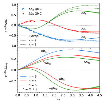
Figure 1: Top: Virial coefficients $\Delta b_{n}$ for $n=2-5$ for the 1D attractive Fermi gas as a function of the dimensionless coupling $\lambda_{1}$. To fit the scale, the $\Delta b_{n}$s are scaled by $\exp(-q\beta\epsilon_{b})$, where $q$ is the maximum number of spin-$\uparrow\downarrow$ pairs. The $k=2$ results are shown as dashed lines, $k=3$ as dashed-dotted lines, and the $k\to\infty$ extrapolation with solid lines. Results for $\Delta b_{3}$ appear in blue, $\Delta b_{4}$ in red, and $\Delta b_{5}$ in green. Blue squares and red stars show the QMC results for $\Delta b_{3}$ and $\Delta b_{4}$, respectively, from Ref. ShillDrut . Bottom: Subspace contributions $\Delta b_{mj}$ as functions of the coupling strength, scaled by $\exp(-j\beta\epsilon_{b})$. Our results are shown as error bands, color-coded as in the top plot by $n=m+j$: blue for $-\Delta b_{21}$, red for $\Delta b_{31}$ and $\Delta b_{22}$, and green for $-\Delta b_{41}$ and $-\Delta b_{32}$. Specific cases are inverted in sign for clarity and to avoid overlaps.

Solving for $\tilde{C}$ in terms of $\Delta b_{2}$ at $k=2$, we find

$$\tilde{C}=2^{-\frac{d}{2}}\left(\sqrt{1+2^{\frac{d}{2}+1}\Delta b_{2}}-1\right),$$ (40)

where we have chosen the solution that yields a real and positive value for $\tilde{C}$, which corresponds to attractive interactions and thus positive $\Delta b_{2}$. Using that result yields $\Delta b_{3}$, $\Delta b_{4}$, and $\Delta b_{5}$ in terms of $\Delta b_{2}$. In the sections that follow we will use the above formulas and their generalizations to $k=3$ and beyond to display the behavior of virial coefficients as $k$ is increased and compare those results with the extrapolations to the large-$k$ limit.

IV Extrapolated Results

In this section we focus on the physically relevant cases of 1D, 2D, and 3D attractive Fermi gases, extrapolating to the large-$k$ (i.e. continuous-time) limit. Specifically, we calculated the interaction-induced changes in the virial coefficients $\Delta b_{3}$ up to $k=21$, $\Delta b_{4}$ up to $k=12$ and $\Delta b_{5}$ up to $k=9$, and based on those results we extrapolated to $k\to\infty$ using the techniques discussed in Ref. HouDrut .

In each spatial dimension, we discuss applications centered around measurable quantities such as the density equation of state, Tan contact, and the isothermal compressibility. The applicability and usefulness of the calculated coefficients extends well beyond those observables, however, as the $\Delta b_{n}$ also determine the high-temperature behavior of a broad suite of thermodynamic quantities such as the energy, entropy, pressure, magnetic susceptibility, etc. Furthermore, we focus largely on unpolarized systems (the exceptions being the density equation of state in 1D and 3D at unitarity), but provide the subspace decomposition of $\Delta b_{4}$ and $\Delta b_{5}$, which extend the applicability of our results to the polarized-system version of the aforementioned thermodynamic quantities.

IV.1 Virial coefficients in 1D

To calculate the virial coefficients of attractively interacting fermions in 1D we used the technique described above combined with the exact Beth-Uhlenbeck result BU ; EoS1D

$$\Delta b_{2}^{\text{1D,exact}}=-\frac{1}{2\sqrt{2}}+\frac{e^{\lambda_{1}^{2}/4}}{2\sqrt{2}}[1+\text{erf}(\lambda_{1}/2)].$$ (41)

This equation, together with Eq. (40) (and its counterparts at higher $k$), allows us to obtain $\tilde{C}$ as a function of the dimensionless physical coupling $\lambda_{1}=2\sqrt{\beta}/a_{0}$, where $a_{0}$ is the 1D scattering length.

The results of our 1D calculations are shown in Fig. 1 and are in excellent agreement with the QMC data of Ref. ShillDrut for $\Delta b_{3}$ and $\Delta b_{4}$. For the latter, the QMC calculations are very limited and stop beyond at $\lambda_{1}\simeq 1.0$ (where the QMC method begins to break down), whereas our present results go well beyond that region. Because a two-body bound state forms in this system as soon as the interaction is turned on, the virial coefficients will tend to grow exponentially with the binding energy (as is evident at second order from the Beth-Uhlenbeck formula). To capture that behavior, we scaled our virial coefficients by the inverse Boltzmann weight $\exp(-q\beta\epsilon_{B})$ of the available particle pairs $q$ (i.e. $q=1$ for $\Delta b_{3}$ and $q=2$ for $\Delta b_{4}$ and $\Delta b_{5}$), where $\epsilon_{B}=1/a_{0}^{2}$ is the binding energy of the two-body system. The resulting mild behavior at strong coupling shows that indeed the scaling factor captures the shape of $\Delta b_{n}$ as the coupling is increased. Beyond that leading contribution, however, $\Delta b_{3}$ is controlled by the atom-dimer scattering properties, just as $\Delta b_{4}$ is controlled by dimer-dimer properties, and so on. In all the dimensions explored here, we found that $\Delta b_{3}$ is of constant sign, whereas $\Delta b_{4}$ and $\Delta b_{5}$ change sign at strong enough coupling, as a result of the competition between positive and negative contributions coming from the fixed-polarization subspaces $\Delta b_{mj}$.

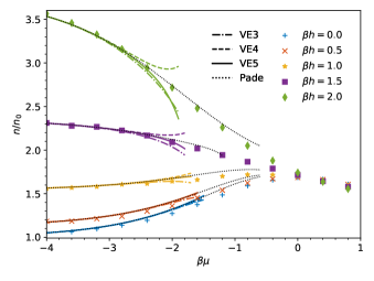
Figure 2: Density equation of state $n$ of the attractive 1D Fermi gas, shown in units of the noninteracting, unpolarized counterpart $n_{0}$ with coupling strength $\lambda_{1}=1.0$, for several values of the chemical potential difference $\beta h=\beta(\mu_{\uparrow}-\mu_{\downarrow})/2$. The colored symbols are complex-Langevin results from Ref. LoheacDrutBraun and the colored lines show the virial expansion at various orders: dashed-dotted line at third order (VE3), dashed line at fourth order (VE4), and solid line at fifth order (VE5). The black dotted line is the result of the $[3/2]$ Padé resummation (see Sec. IV.7). The Padé approximant for $\beta h=1.5$ contains a pole close to $\beta\mu=-1.2$; the corresponding dotted line is therefore cut off at that value. The limiting value for $\beta\mu\to-\infty$ is known exactly and is given by $\cosh(\beta h)$.

The $\Delta b_{mj}$ are shown in the bottom panel of Fig. 1. There is naturally only one subspace contributing at third order: $\Delta b_{3}=2\Delta b_{21}$. However, $\Delta b_{4}=\Delta b_{22}+2\Delta b_{31}$ and $\Delta b_{5}=2\Delta b_{32}+2\Delta b_{41}$. Furthermore, in each of the latter, the subspace terms enter with similar magnitudes but opposing signs, and thus compete to determine the sign and size of $\Delta b_{n}$. It is hard to miss that $|\Delta b_{m1}|$ follows essentially the same trend as a function of the coupling across all $m$, and that trend becomes increasingly suppressed for increasing $m$. A similar observation applies to $|\Delta b_{m2}|$. The suppression with increased polarization is easy to understand: at large $m$ both $|\Delta b_{m1}|$ and $|\Delta b_{m2}|$ must approach the noninteracting values (i.e. zero) as the majority of the particles do not interact due to Pauli blocking.

IV.2 Applications in 1D

IV.2.1 Density equation of state at finite polarization

In the virial expansion, the density equation of state of a polarized system becomes a double series expansion in powers of the fugacity of each spin $z_{s}=\exp(\beta\mu_{s})$, $s=\uparrow,\downarrow$. More specifically, the grand thermodynamic potential $\Omega=\Omega_{0}+\Delta\Omega$, relative to its noninteracting counterpart $\Omega_{0}$ becomes

$$-\beta\Delta\Omega=Q_{1}\sum_{n=2}^{\infty}\sum_{\begin{subarray}{c}m,j>0\\ m+j=n\end{subarray}}\Delta b_{mj}z_{\uparrow}^{m}z_{\downarrow}^{j},$$ (42)

such that the particle number density for spin-$\uparrow$ is given by

$$\lambda_{T}^{d}n_{\uparrow}=\lambda_{T}^{d}n_{\uparrow,0}+2\sum_{n=2}^{\infty}\sum_{\begin{subarray}{c}m,j>0\\ m+j=n\end{subarray}}m\Delta b_{mj}z_{\uparrow}^{m}z_{\downarrow}^{j},$$ (43)

where $\lambda_{T}=\sqrt{2\pi\beta}$ is the thermal wavelength, $\lambda_{T}^{d}n_{\uparrow,0}=f_{d/2}(z_{\uparrow})$ is the noninteracting value in $d$ dimensions, $f_{d/2}(z)=\text{Li}_{d/2}(-z)$ is the Fermi-Dirac function, and $\text{Li}_{s}(x)$ is the polylogarithm function. An analogous expression to Eq. (43) holds for $\lambda_{T}^{d}n_{\downarrow}$.

In Fig. 2 we show our estimates for the density equation of state at finite polarization in the virial expansion, for attractively interacting fermions in 1D. We compare our results with those of Ref. LoheacDrutBraun obtained with the complex Langevin method. The fifth-order virial expansion provides a modest improvement over the third and fourth orders. However, for all the available polarizations the agreement with the data is reasonable as long as $\beta\mu$ is sufficiently small. Resummation techniques (see below) like Padé approximants extend that agreement (which while not perfect, it is better than qualitative) with the available data over a wider $\beta\mu$ region.

IV.2.2 Contact

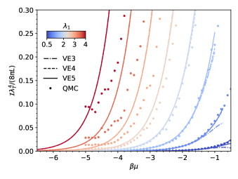
Figure 3: Tan contact $\mathcal{I}$, in the dimensionless form $\mathcal{I}\pi\beta^{2}/(2L\lambda_{1}^{2})$, as a function of $\beta\mu$, for the attractive 1D Fermi gas. The color encodes the coupling strength of from $\lambda_{1}=0.5$ (dark blue) to $\lambda_{1}=4.0$ (dark red) in steps of $0.5$. The dots show the QMC results of Ref.EoS1D and the curves show the virial expansion at various orders, following the same line style as in Fig. 2.

As elucidated by Tan and others ShinaTan1 ; ShinaTan2 ; ShinaTan3 , in systems with short-range interactions the short-distance and high-frequency behavior of correlation functions is captured by a single quantity called the contact, often denoted by $\mathcal{I}$. The contact also enters celebrated pressure-energy and other exact relations as well as sum rules ZhangLeggett ; Werner ; BraatenPlatter1 ; BraatenPlatter2 ; BraatenPlatter3 ; SonThompson ; TaylorRanderia ; BraatenReview ; Valiente1 ; Valiente2 ; WernerCastin ; McKenneyDrut ; ValientePastukhov and is therefore a crucial piece of the thermodynamic puzzle that complements conventional quantities. Below, we compare our virial-expansion results for the contact in 1D with QMC data.

In 1D, the contact is given by

$$\mathcal{I}=\frac{2}{\beta}\frac{\partial(\beta\Omega)}{\partial a_{0}},$$ (44)

such that its virial expansion becomes

$$\mathcal{I}=\frac{4\pi}{\lambda^{3}_{T}}Q_{1}\sum_{m=2}^{\infty}c_{m}z^{m},$$ (45)

where $\lambda_{T}=\sqrt{2\pi\beta}$ and

$$c_{m}=\sqrt{\frac{\pi}{2}}\lambda_{1}^{2}\frac{\partial\Delta b_{m}}{\partial\lambda_{1}}.$$ (46)

The Beth-Uhlenbeck formula yields

$$c_{2}=\frac{\lambda_{1}^{2}}{4}+\frac{\sqrt{\pi}}{8}e^{\lambda_{1}^{2}/4}\lambda_{1}^{3}[1+\text{erf}(\lambda_{1}/2)],$$ (47)

as first shown in Ref. EoS1D . Using the $\lambda_{1}$ dependence of our results for $\Delta b_{n}$, we obtained the virial expansion of $\mathcal{I}$ up to fifth order. In Fig. 3 we show the dimensionless, intensive form of the contact, $\mathcal{I}\pi\beta^{2}/(2L\lambda_{1}^{2})$ as a function of temperature in the virial expansion. At weak couplings ($\lambda_{1}\leq 2.0$), the virial expansion shows good agreement with the QMC results of Ref.EoS1D . However, as the coupling strength increases, the disparity becomes significant, which is not completely unexpected as both methods face challenges in the strong coupling regime: the radius of convergence of the virial expansion can be very small, such that the expansion ceases to be useful even at very negative $\beta\mu$; on the other hand, the lattice QMC method may suffer from increasing lattice-spacing effects at strong coupling, due to the reduced size of the two-body bound state.

IV.3 Virial coefficients in 2D

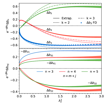
Figure 4: Top: Virial coefficients $\Delta b_{n}$ for $n=2-5$ for the 2D attractive Fermi gas, as a function of the square of the dimensionless coupling $\lambda_{2}$. To fit the scale, $\Delta b_{n}$s are scaled by $\exp(-q\beta\epsilon_{b})$, where $q$ is the maximum number of spin-$\uparrow\downarrow$ pairs, and $\Delta b_{mj}$s are scaled by $\exp(-j\beta\epsilon_{b})$. The $k=2$ results are shown as dashed lines, $k=3$ as dashed-dotted lines and the $k\to\infty$ extrapolation with solid lines. Results for $\Delta b_{3}$ appear in blue, for $\Delta b_{4}$ in red, and for $\Delta b_{5}$ in green. The diagrammatic result for $\Delta b_{3}$ from Ref. virial2D2 appear as blue dots. Bottom: Subspace contributions $\Delta b_{mj}$ as functions of the coupling strength. Our results are shown as error bands, color-coded as in the top plot by $n=m+j$: blue for $-\Delta b_{21}$, red for $\Delta b_{31}$ and $\Delta b_{22}$, and green for $-\Delta b_{41}$ and $-\Delta b_{32}$.

In Fig. 4 we show our results for $\Delta b_{n}$ for the 2D Fermi gas with attractive interactions Theory2D . As in 1D, we scaled the coefficients by $\exp(-q\beta\epsilon_{B})$, where $q$ is the maximum number of available spin-$\uparrow\downarrow$ pairs. To renormalize, we again rely on the exact Beth-Uhlenbeck result BU ; DrummondVirial2D ; virial2D ; virial2D2 ; PhysRevA.89.013614 ; Ordo ; Daza2D

$$\Delta b_{2}^{\text{2D,exact}}=e^{\lambda_{2}^{2}}-\int_{0}^{\infty}\frac{dy}{y}\frac{2e^{-\lambda_{2}^{2}y^{2}}}{\pi^{2}+4\ln^{2}y},$$ (48)

to define $\tilde{C}$ as a function of the physical coupling $\lambda^{2}_{2}=\beta\epsilon_{B}$, where $\epsilon_{B}$ is the binding energy of the two-body system.

At all orders the similarity with 1D is clear: $\Delta b_{3}$ remains negative for all the couplings studied, whereas $\Delta b_{4}$ and $\Delta b_{5}$ change sign at strong enough coupling as a result of a competition between subspaces $\Delta b_{m1}$ and $\Delta b_{n2}$ governed by the number of spin-$\uparrow\downarrow$ pairs available in each subspace. While $\Delta b_{4}$ and $\Delta b_{5}$ are calculated here for the first time (thus furnishing a prediction), $\Delta b_{3}$ was calculated in Ref. virial2D2 . The results of the latter are shown in Fig. 4 with blue dots, which agree remarkably well with our answers.

The subspace contributions $\Delta b_{mj}$ are shown in the bottom panel of Fig. 4 and we again note clear parallels with the 1D case. Specifically, the subspace terms contributing to $\Delta b_{4}$ and $\Delta b_{5}$ enter with similar magnitudes but opposing signs, indicating that the final results for $\Delta b_{4}$ and $\Delta b_{5}$ result from subtle coupling-dependent cancellations. Furthermore, $|\Delta b_{m1}|$ and $|\Delta b_{m2}|$ follow consistent trends as a function of the coupling across all $m$ (with the expected suppression as $m$ is increased). In fact, once the $\exp(-q\beta\epsilon_{B})$ factor is included, $|\Delta b_{m1}|$ and $|\Delta b_{m2}|$ are approximately constant as the coupling is increased.

At weak coupling, on the other hand, the details are elusive in the scale of Fig. 4. There, non-perturbative effects are only visible if shown differently, as we do in Fig. 5, where show that, as functions of $\Delta b_{2}$ all the coefficients tend smoothly to zero as the coupling is weakened. The non-perturbative behavior at weak coupling is completely captured by $\Delta b_{2}$.

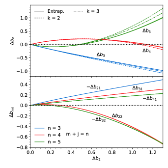
Figure 5: Weak-coupling zoom-in on Fig. 4, not including the $\exp(-q\beta\epsilon_{B})$ factor and plotted as a function of $\Delta b_{2}$. The right edge of the horizontal axis corresponds to $\lambda_{2}\simeq 0.588$.

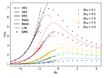
Figure 6: Density equation of state $n$, shown in units of the noninteracting counterpart $n_{0}$ at different coupling strength $\lambda_{2}^{2}=\beta\epsilon_{B}$ in 2D. The colored dots are the QMC results from Ref. AndersonDrut , the colored thin line shows the Luttinger-Ward result of Ref. LWDensity2D , and the colored thick lines are virial expansions at different orders (same line style as in previous Fig. 2). The black dotted lines and dashed lines are the results, respectively, of Padé and Borel resummation of order $[3/2]$ (see Sec. IV.7) using the virial coefficients up to the fifth order.

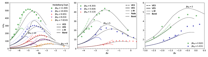
Figure 7: Density equation of state $n$ of the 2D attractive Fermi gas, shown in units of the noninteracting counterpart $n_{0}$ at different coupling strength $\lambda_{2}^{2}=\beta\epsilon_{B}$ in 2D. The colored symbols are the results of experimental analyses from Ref. Exp4 and the colored lines show the virial expansion at different orders (following the same line style as in previous figures). [Note: the fourth-order case is omitted from this figure only for the clarity.] The black dashed lines are the results of Borel resummation of order $[3/2]$ (see Sec. IV.7) using coefficients up to the fifth order. The thin black solid lines are the Luttinger-Ward results of Ref. LWDensity2D , around which the nearby labels indicate the corresponding $\beta\epsilon_{B}$. Only the central value of our estimates is used in these plots; the relative-error on the virial coefficients from continuous-time extrapolation can reach 15% at the strongest couplings shown in the left panel, although that does not translate into a significant change in the scale shown. Also in the left panel, the blue dotted lines show our Borel-resummed results at $\beta\epsilon_{B}=9.5$ (lower) and 10.5 (upper) respectively, which enclose the experimental points completely (in agreement with the experimental uncertainty on $\beta\epsilon_{B}$). In the middle panel, we also present the [3/2] Padé result as a black dotted line for $\beta\epsilon_{B}=6.3$ to demonstrate the performance difference between the two resummation techniques at strong coupling. Reference Exp4 also provides data at $\beta\epsilon_{B}=0.45(5)$, but mostly at large $\beta\mu>0$ and therefore not shown here.

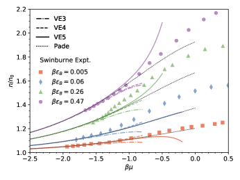
Figure 8: Density equation of state $n$, shown in units of the noninteracting counterpart $n_{0}$ at different coupling strength $\lambda_{2}^{2}=\beta\epsilon_{B}$ in 2D. The colored symbols are the results of experimental analyses from Ref. Exp3 and the colored lines are virial expansions at different orders (the same line style applied). The black dotted lines and dashed lines are the results, respectively, of Padé and Borel resummation (see Sec. IV.7) of order $[3/2]$ using coefficients up to the fifth order.

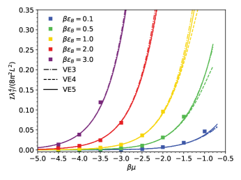
Figure 9: Contact $\mathcal{I}$, represented in the dimensionless form $\mathcal{I}\lambda_{T}^{4}/(8\pi^{2}L^{2})$, as a function of $\beta\mu$ in 2D. The colored squares are the QMC results of Ref. AndersonDrut and the colored lines are the results of virial expansion at various orders.

IV.4 Applications in 2D

IV.4.1 Density equation of state at zero polarization

Equation (43) can be easily applied in the unpolarized case by setting $z_{\uparrow}=z_{\downarrow}$, such that the total density is given by

$$\lambda_{T}^{d}n=\lambda_{T}^{d}n_{0}+2\sum_{n=2}^{\infty}n\Delta b_{n}z^{n},$$ (49)

where the factor of $2$ accounts for the number of species. Our results for $\Delta b_{n}$ yield the curves shown in Fig. 6, where they are compared with the QMC results of Ref. AndersonDrut and the Luttinger-Ward results of Ref. LWDensity2D . The agreement with the QMC data is outstanding. Moreover, for all the couplings in the figure the Padé and Borel resummations substantially extend the region of agreement. With the exception of the weakest coupling in the figure (where the QMC results likely incur volume effects due to the large size of the two-body bound state), the virial expansion is systematically closer to the QMC data than to the Luttinger-Ward results. Although small, this discrepancy remains unresolved.

In Figs. 7 and 8, we compare our results with the experimental data of Refs. Exp4 and Exp3 , respectively. In all cases, the agreement is remarkable in the regions where the virial expansion is expected to work. Naturally, that region is pushed to progressively more negative $\beta\mu$ as the coupling is increased; in other words, the radius of convergence of the virial expansion decreases as the coupling increases. However, it is also clear that, beyond weak and intermediate couplings (roughly up to $\beta\epsilon_{B}=3.0$), the benefits of pushing the virial expansion up to fifth order start to diminish, if the virial expansion is taken at face value. We find, on the other hand, that Padé and Borel resummations dramatically enhance the usefulness of the virial coefficients. As shown in Fig. 7 (left and center panels in particular), our Borel resummations of the virial expansion agree not only qualitatively but in several cases also quantitatively with the experimental data.

IV.4.2 Contact

In 2D, the contact is defined as

$$\mathcal{I}=\frac{2\pi}{\beta}\frac{\partial(\beta\Omega)}{\partial\ln(a_{0}/\lambda_{T})},$$ (50)

such that its virial expansion becomes

$$\mathcal{I}=\frac{(2\pi)^{2}}{\lambda_{T}^{2}}Q_{1}\sum_{m=2}^{\infty}c_{m}z^{m},$$ (51)

where

$$c_{m}=\lambda_{2}\frac{\partial\Delta b_{m}}{\partial\lambda_{2}}.$$ (52)

The Beth-Uhlenbeck formula yields

$$c_{2}=2\lambda_{2}^{2}e^{\lambda_{2}^{2}}\left[1+2\int_{0}^{\infty}\differential y\frac{ye^{-\lambda_{2}^{2}(y^{2}+1)}}{\pi^{2}+4\ln^{2}y}\right],$$ (53)

as shown in Refs. virial2D2 ; AndersonDrut . Using the $\lambda_{2}$ dependence of our results for $\Delta b_{n}$, we obtained the virial expansion of $\mathcal{I}$ up to fifth order. In Fig. 9 we show the dimensionless, intensive form of the contact, $\mathcal{I}\lambda_{T}^{4}/(8\pi^{2}L^{2})$, as a function of $\beta\mu$ in the virial expansion and compared with the QMC results from Ref. AndersonDrut . As with the equation of state shown above, the agreement with the QMC data is remarkable in the region where the virial expansion is expected to work well.

IV.5 Virial coefficients in 3D

Finally, in 3D we have BU ; LeeSchaeferPRC1

$$\Delta b_{2}^{\text{3D,exact}}=\frac{e^{\lambda_{3}^{2}}}{\sqrt{2}}[1+\mbox{erf}(\lambda_{3})],$$ (54)

where $\lambda_{3}=\sqrt{\beta}/a_{0}$, and $a_{0}$ is the s-wave scattering length. Note the unitary limit corresponds to $\lambda_{3}=0$ and we only explore $\lambda_{3}<0$ regime in this work.

In Fig. 10 and Fig. 11, we present our results for $\Delta b_{n}$ for the 3D Fermi gas with attractive interactions. These plots parallel the main figure of our previous work of Ref. HouDrut , where we show the same results as a function of $\Delta b_{2}$. For completeness, future reference, and to parallel our discussion in lower dimensions, Fig. 10 shows our results as a function of $-1/\lambda_{3}$ to display the weak coupling regime, while in Fig. 11 we plot the approach to the unitary limit ($\lambda_{3}=0$) as a function of $\lambda_{3}$. In the latter, we find excellent agreement with the exact $\Delta b_{3}$ of Ref. Leyronas (see also Refs. LiuHuDrummond ; DBK ; Rakshit ; Ngampruetikorn ).

The bottom panels of Fig. 10 and 11 show the subspace decomposition of $\Delta b_{n}$ into $\Delta b_{mj}$. The qualitative similarities with lower dimensions are clear. Here, however, we have explored a coupling regime in which no two-body bound states are yet formed, such that the introduction of the $\exp(-q\beta\epsilon_{B})$ factor is not needed. As the unitary limit is approached, however (see left edge of Fig. 11), all of the coefficients we computed start to display increased curvature. Beyond that point, we expect an exponential increase characterized by $\exp(q\beta\epsilon_{B})$ precisely as in lower dimensions. The rapid downturn of $\Delta b_{3}$ at strong coupling was, in fact, already noticed in Ref. Leyronas , while the same feature for $\Delta b_{4}$ appeared in Ref. Ngampruetikorn . Here, we see that that behavior is inevitable as it is merely a consequence of the dominance of $\Delta b_{m2}$ (with $m=2,3$) over $\Delta b_{m1}$ (with $m=3,4$). However, the sign difference between these terms, as in lower dimensions, results in cancellations that make fully numerical determinations of $\Delta b_{4}$ and $\Delta b_{5}$ a difficult task. Finally, we note that our analysis of $\Delta b_{mj}$, and their apparent systematic behavior, suggests that the conjecture of Ref. Bhaduri1 ; Bhaduri2 on the high-order virial coefficients in the unitary limit may be refined by focusing on the subspaces rather than the full $\Delta b_{n}$.

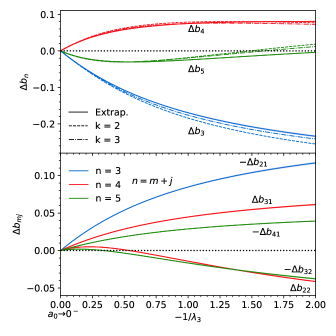
Figure 10: $\Delta b_{n}$ for $n=2-5$ for the 3D Fermi gas in the weak-coupling regime, as a function of the dimensionless coupling $\lambda_{3}$. The $k=2$ results are shown with dashed lines, $k=3$ with dashed-dotted lines, and the $k\to\infty$ extrapolation with solid lines. Results for $\Delta b_{3}$ appear in blue, for $\Delta b_{4}$ in red, and for $\Delta b_{5}$ in green.

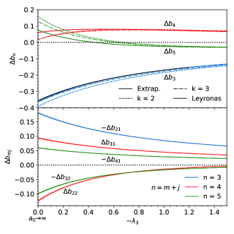
Figure 11: $\Delta b_{n}$ for $n=2-5$ for the 3D Fermi gas in the strong-coupling regime, as a function of the dimensionless coupling $\lambda_{3}$. [Note that the unitary limit corresponds to $\lambda_{3}=0$.] The exact result for $\Delta b_{3}$ from Ref. Leyronas appears as a thin solid black line. The $k=2$ results are shown with dashed lines, $k=3$ with dashed-dotted lines, and the $k\to\infty$ extrapolation with solid lines. Results for $\Delta b_{3}$ appear in blue, for $\Delta b_{4}$ in red, and for $\Delta b_{5}$ in green.

IV.6 Applications in 3D

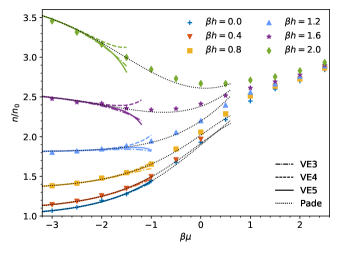
Figure 12: Density equation of state $n$ of the unitary Fermi gas, shown in units of the noninteracting, unpolarized counterpart $n_{0}$, for several values of the chemical potential difference $\beta h=\beta(\mu_{\uparrow}-\mu_{\downarrow})/2$. The colored symbols are complex-Langevin results from Ref. polarizedUFGCL and the colored lines show the virial expansion at various orders: dashed-dotted line at third order, dashed line at fourth order, and solid line at fifth order. The black dotted line is the result of the $[3/2]$ Padé resummation (see Sec. IV.7). The limiting value for $\beta\mu\to-\infty$ is known exactly and is given by $\cosh(\beta h)$.

IV.6.1 Density equation of state in the unitary limit

In Fig. 12, we present our results for the density equation of state in the unitary limit and compare with the complex-Langevin results of Ref. polarizedUFGCL . The fifth-order expansion shows the best agreement compared to its lower-order counterparts, although the improvement is mostly marginal. When applying the Padé resummation technique, however, the agreement with the data is extended even beyond $\beta\mu=0$. Notably, the change in curvature displayed by the data is reproduced by the Padé approximant. Beyond $\beta\mu=0.6$, however, the Padé approximant progressively departs from the data. The Borel-Padé resummation shows performance very similar to that of pure Padé resummation and is therefore omitted.

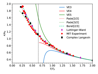
Figure 13: Compressibility $\kappa$ of the unitary Fermi gas in units of its noninteracting, ground-state counterpart $\kappa_{0}$, as a function of the temperature $T$ in units of the Fermi temperature $T_{F}$. Our results for the virial expansion for fugacity $z\in[0,1]$ are shown as solid lines: blue for third order, red for fourth order, and green for fifth order. The dotted lines are the result of Padé resummation of order [2/2] (red) and [3/2] (green), respectively. The cyan dashed line is the result of a [2/3] Borel-Padé resummation (see Sec. IV.7). Other resummation orders are omitted due to the appearance of poles on the real axis in the region of interest. The vertical dotted line corresponds to the approximate $T/T_{F}$ where $z=1$ for the three resummed results. The red circles show the data from the MIT experiment of Ref. Exp2 . The purple diamonds are the Luttinger-Ward calculations of Ref. EnssHaussmann . The black squares are complex-Langevin results from Ref. polarizedUFGCL .

IV.6.2 Compressibility in the unitary limit

The compressibility $\kappa$ is defined as

$$\kappa=-\frac{1}{V}\left[\partialderivative{V}{P}\right]_{T}=\frac{\beta}{n^{2}}\left[\partialderivative{n}{\beta\mu}\right]_{T},$$ (55)

where, in terms of virial expansion,

$$\partialderivative{n}{(\beta\mu)}=\partialderivative{n_{0}}{(\beta\mu)}+\sum_{m=2}^{\infty}m^{2}\sum_{i+j=m}\Delta b_{ij}z_{\uparrow}^{i}z_{\downarrow}^{j}.$$ (56)

In Fig. 13, we present our estimates for the compressibility $\kappa$, shown in units of its noninteracting counterpart $\kappa_{0}=3/(2n\epsilon_{F})$, in the unitary limit and compare them with the experimental measurements from Ref. Exp2 , the Luttinger-Ward calculations of Ref. EnssHaussmann , and the complex-Langevin results from Ref. polarizedUFGCL ,

The results of Padé and Borel-Padé resummations show much better agreement with experimental data than the finite-order virial expansion, even well beyond the region of the virial expansion $z\ll 1$. Specifically, the resummations smoothly follow the trend of the experimental data up to fugacities as large as $z=10$ (maximum fugacity shown in Fig. 13), which is surprising considering that the superfluid transition occurs at $z\simeq 10$.

IV.6.3 Tan contact

For completeness, we cite the equations for the contact and its virial expansion, as done above in 1D and 2D. Our results for the contact at unitarity are presented elsewhere HouDrut . In 3D, the contact is defined as

$$\mathcal{I}=-\frac{4\pi}{\beta}\frac{\partial(\beta\Omega)}{\partial a_{0}^{-1}},$$ (57)

such that its virial expansion reads

$$\mathcal{I}=\frac{8\pi^{2}}{\lambda_{T}}Q_{1}\sum_{m=2}^{\infty}c_{m}z^{m},$$ (58)

where

$$c_{m}=\frac{1}{\sqrt{2\pi}}\frac{\partial\Delta b_{m}}{\partial\lambda_{3}}.$$ (59)

The Beth-Uhlenbeck formula yields

$$c_{2}=\frac{1}{\pi}+\frac{1}{\sqrt{\pi}}\lambda_{3}\;e^{\lambda_{3}^{2}}(1+\text{erf}(\lambda_{3})).$$ (60)

IV.7 Resummation techniques

Before concluding, we present more details on the resummation techniques used in this work, namely the Padé and Borel-Padé resummations, which we have found useful in extending the applicability of the virial expansion. Generally speaking, the Padé resummation, based on fitting a Padé approximant (see below), is useful when a series is finitely truncated, as in the case of virial expansion. In such cases, the Padé approximant is often better behaved than the partial sums of the original series, and it may even work where the original series diverges, i.e. beyond the radius of convergence of the series. In our case, the technique is simple to apply: the coefficients $\Delta b_{n}$ that we calculated determine the unknown coefficients of a Padé approximant which is a rational function $P(z)/Q(z)$, where $P$ and $Q$ are polynomials of degrees $a$ and $b$ respectively. Such an approximant is denoted by $[a/b]$. Using $m$ available virial coefficients, it is possible to fully determine $m$ coefficients in $P$ and $Q$, which means that $a+b=m$ (note that the independent term in $Q$ is set to 1 by convention). By definition, the Taylor expansion of $P(z)/Q(z)$ at small $z$ reproduces the input virial coefficients.

The Borel-Padé resummation is based on applying a Borel summation BorelSum1 ; BorelSum2 , followed by a Padé fit and reverse (integral) Borel transform (which is a Laplace transform). In short, the Borel summation amounts to replacing each coefficient $\Delta b_{n}$ by $\Delta b_{n}/n!$; the resulting function is fit with a Padé approximant, and that approximant is then numerically integrated to (effectively) undo the introduction of the $n!$ factor. Further details on this well-known technique can be found, for instance, in the Supplemental Materials of Ref. HouDrut .

Such an approach has been applied in many other areas (famously in the calculation of critical exponents GuidaJustin ) ranging from QCD QCDBorelPade to ultracold atomic physics NishidaSon ; ArnoldDrutSon . The method is particularly useful for summing diverging asymptotic series, which is the reason we used it in 2D at strong coupling. In fact, our empirical observations are that the Borel-Padé resummation yields better qualitative behavior and better overall agreement with experiments at strong coupling than the pure Padé fit mentioned above (see middle panel of Fig. 7). At weak coupling, on the other hand, both techniques yield similar results (see, e.g., Fig. 6). In 3D, the strongest effective coupling corresponds to the unitary limit; beyond that point the strong attraction leads to the formation of bosonic dimers whose interaction is, as a residual effect, weakly repulsive. However, the two resummation methods still yield similar results at unitarity as the magnitude of the virial coefficients is small. It is only for positive $\lambda_{3}$ (corresponding to deeply bound pairs) that $\Delta b_{n}$ will start to grow exponentially, as we saw in 1D and 2D, and in that case the Borel-Padé resummation is expected to offer better estimates.

In Fig. 14, we show in more detail a comparison of Padé and Padé-Borel resummations at different orders, as applied to the density equation of state of the 2D attractive Fermi gas. For all couplings, the pure Padé approach of order $[3/2]$ shows the best agreement with the QMC calculations compared with every other lower-order approximant.[For the $[1/4]$ approximant we have found no solution for the Padé coefficients f or the given values of the virial coefficients.] We find that, for $\beta\epsilon_{B}=2.0$ and $3.0$, the $[3/1]$ approximant encounters poles on the positive $z$ axis at $\beta\mu\approx-2.7$ and $-1.7$ respectively, which underscores the importance of calculating high-order virial coefficients in order to access a wide range of possible Padé approximants.

Although we found remarkable agreement between our resummations and other results in several examples, these techniques admittedly represent a break from the main a priori method we used to obtain the virial coefficients, as Padé and Borel methods have not been rigorously justified here (to the best of our knowledge). Future studies may shed light on this matter.

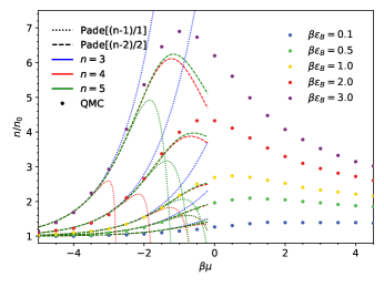
Figure 14: Density equation of state $n$, shown in units of the noninteracting counterpart $n_{0}$ at different coupling strength $\lambda_{2}^{2}=\beta\epsilon_{B}$ in 2D. The colored dots are the QMC results from Ref. AndersonDrut , the colored lines shows the results using Padé approximation at different orders. Different colors indicate the higher order of coefficients used in calculating the Padé approximant: blue for $n=3$, red for $n=4$ and green for $n=5$; different linestyles represent the degree of denominator in the approximant: dotted line for $[(n-1)/1]$ and dashed line for $[(n-2)/2]$.

V Summary and Conclusions

In this work we calculated the interaction-induced change in the third to fifth virial coefficients, $\Delta b_{3}$ – $\Delta b_{5}$, of spin-$1/2$ fermions with attractive interactions using a temporal lattice approximation. We provided a few analytic answers in coarse discretizations $k=1,2$ before pushing our results to high $k$ ($k=21$ for $\Delta b_{3}$; $k=12$ for $\Delta b_{4}$; and $k=9$ for $\Delta b_{5}$) and extrapolating to the continuous-time limit. Using a renormalization prescription based on matching $\Delta b_{2}$ to the known exact results, we obtained $\Delta b_{n}$ for $n=3,4,5$ for a range of attractive couplings in 1D, 2D, and 3D.

In 1D, our results for $\Delta b_{n}$ agree with previous QMC estimates (obtained at weak coupling) and substantially extend the coupling range. In addition, we obtained the subspace contributions which as in higher dimensions, appear with similar magnitude but opposite sign, thus partially cancelling each other out. We found that the presence of a two-body bound state strongly controls the magnitude of the virial coefficients: multiplying by a factor $\exp(-q\beta\epsilon_{B})$, where $q$ is the maximum number of $\uparrow,\downarrow$ pairs and $\epsilon_{B}$ their binding energy, it is possible to show all the virial coefficients we calculated on the same vertical scale.

As an application in 1D, we compared our results (both partial sums as well as Padé resummation) with complex Langevin results for the density equation of state at finite polarization, where we found excellent agreement. Similarly, we compared with QMC data for the Tan contact in the unpolarized case, where we found very good agreement at weak coupling, deteriorating as the coupling is increased (likely due to the limited range of validity of the expansion, but also due to the decreased quality of the data and possible lattice spacing effects at strong coupling).

In 2D, the exponential growth mentioned above for 1D is even more evident: all the coefficients we calculated become very approximately constant once the $\exp(-q\beta\epsilon_{B})$ factor is included. The well-known nonperturbative features of this system at weak coupling are smoothly captured by plotting as a function of $\Delta b_{2}$ rather than $\lambda_{2}^{2}=\beta\epsilon_{B}$. Our results for $\Delta b_{3}$ match very closely those of Ref. virial2D2 .

As an application in 2D, we compared our results with QMC and experimental data on the density equation of state of the unpolarized system. Partial sums of the virial expansion and resummation results are in excellent agreement with QMC data for a range of negative values of $\beta\mu$, as expected. Furthermore, in all cases the fifth-order of the virial expansion yields an improvement over lower orders. Beyond partial sums, the Padé and Padé-Borel resummation shows outstanding agreement in a range of $\beta\mu$ that is substantially larger than that of the partial sums. When comparing with experimental data, the picture is similar: the partial sums give at least reasonable agreement where expected, but it is the Padé-Borel resummation that brings about the most remarkable overall agreement with the data. Finally, our comparison with the Tan contact obtained by QMC methods, where available, shows excellent agreement.

In 3D, we calculated $\Delta b_{n}$ for couplings up to the unitary limit. Our results for $\Delta b_{3}$ show remarkable agreement with the exact result of Ref. Leyronas at all couplings. For the unitary limit, our results were discussed at length elsewhere HouDrut . As no bound states are formed for the couplings we explored in 3D, there is no need to include an exponential factor as in the 1D and 2D cases; the growth of the virial coefficients is in fact relatively mild for all the couplings we explored in 3D.

As an application in 3D, we have calculated the density equation of state at finite chemical potential asymmetry, as well as the compressibility of the unpolarized system. As in the 1D case, we find that the Padé resummation substantially extends the usefulness of the virial expansion. In particular, for the compressibility the agreement with experiments extends as far as $z=10$.

In 1D, 2D, and 3D we presented not only $\Delta b_{n}$ for $n=3,4,5$, but also the subspace contributions, crucially $\Delta b_{m1}$ and $\Delta b_{m2}$. Discerning these is important because they determine the thermodynamics of the polarized version of the systems we studied. In particular for $\Delta b_{4}$ and $\Delta b_{5}$ the subspace contributions enter with similar magnitudes but opposing signs in all the cases we studied, indicating that the final answers for those coefficients are the result of potentially delicate, coupling-dependent cancellations.

Finally, it should be pointed that out, although we have shown results for a variety of attractively interacting Fermi gases, our analytic results apply to repulsively interacting cases as well. We defer the analysis of the repulsive case to future work. To facilitate the application of our results to those and other cases, we have made our analytic formulas available in a Python code as Supplemental Material SupMat , along with data tables for the extrapolated virial coefficients.

- (1) S. Giorgini, L.P. Pitaevskii, S. Stringari, Theory of ultracold Fermi gases, Rev. Mod. Phys. 80, 1215 (2008).
- (2) I. Bloch, J. Dalibard, W. Zwerger Many-Body Physics with Ultracold Gases, Rev. Mod. Phys. 80, 885 (2008).
- (3) Ultracold Fermi Gases, Proceedings of the International School of Physics “Enrico Fermi", Course CLXIV, Varenna, June 20 – 30, 2006, M. Inguscio, W. Ketterle, C. Salomon (Eds.) (IOS Press, Amsterdam, 2008).
- (4) C. Chin, R. Grimm, P. Julienne, and E. Tiesinga, Feshbach resonances in ultracold gases, Rev. Mod. Phys. 82, 1225 (2010).
- (5) M. Lewenstein, A. Sanpera, V. Ahufinger, Ultracold Atoms in Optical Lattices: Simulating Quantum Many-body Systems, (Oxford University Press, New York, 2012)
- (6) S. Nascimbene, N. Navon, K. J. Jiang, F. Chevy, and C. Salomon, Exploring the thermodynamics of a universal Fermi gas, Nature (London) 463, 1057 (2010).
- (7) M. J. H. Ku, A. T. Sommer, L. W. Cheuk, and M. W. Zwierlein, Revealing the Superfluid Lambda Transition in the Universal Thermodynamics of a Unitary Fermi Gas, Science 335, 563 (2012).
- (8) I. Boettcher, L. Bayha, D. Kedar, P.A. Murthy, M. Neidig, M.G. Ries, A.N. Wenz, G. Zürn, S. Jochim, and T. Enss, Equation of State of Ultracold Fermions in the 2D BEC-BCS Crossover Region, Phys. Rev. Lett. 116, 045303 (2016).
- (9) K. Fenech, P. Dyke, T. Peppler, M.G. Lingham, S. Hoinka, H. Hu, and C.J. Vale, Thermodynamics of an Attractive 2D Fermi Gas, Phys. Rev. Lett. 116, 045302 (2016).
- (10) X.-J. Liu, Virial expansion for a strongly correlated Fermi system and its application to ultracold atomic Fermi gases, Phys. Rep. 524, 37 (2013).
- (11) C. J. Horowitz and A. Schwenk, The Virial equation of state of low-density neutron matter, Phys. Lett. B 638, 153 (2006).
- (12) C. J. Horowitz and A. Schwenk, The Neutrino response of low-density neutron matter from the virial expansion, Phys. Lett. B 642, 326 (2006).
- (13) C. J. Horowitz and A. Schwenk, Cluster formation and the virial equation of state of low-density nuclear matter, Nucl. Phys. A 776, 55 (2006).
- (14) C. R. Shill, J. E. Drut, Virial coefficients of 1D and 2D Fermi gases by stochastic methods and a semiclassical lattice approximation, Phys. Rev. A 98, 053615 (2018).
- (15) Y. Hou, A. Czejdo, J. DeChant, C. R. Shill, J. E. Drut, Leading- and next-to-leading-order semiclassical approximation to the first seven virial coefficients of spin-1/2 fermions across spatial dimensions, Phys. Rev. A 100, 063627 (2019).
- (16) K. J. Morrell, C. E. Berger, and J. E. Drut Third- and fourth-order virial coefficients of harmonically trapped fermions in a semiclassical approximation, Phys. Rev. A 100, 063626 (2019).
- (17) Y. Hou, J. E. Drut The fourth- and fifth-order virial coefficients from weak-coupling to unitarity, arXiv:2004.08685.
- (18) Supplemental Materials: Python code and data tables.
- (19) E. Beth and G. E. Uhlenbeck, The quantum theory of the non-ideal gas. II. Behaviour at low temperatures, Physica (Utrecht) 4, 915 (1937).
- (20) A. C. Loheac, J. Braun, and J. E. Drut, Polarized fermions in one dimension: Density and polarization from complex Langevin calculations, perturbation theory, and the virial expansion, Phys. Rev. D 98, 054507 (2018).
- (21) M. D. Hoffman, P. D. Javernick, A. C. Loheac, W. J. Porter, E. R. Anderson, and J. E. Drut, Universality in one-dimensional fermions at finite temperature: Density, compressibility, and contact, Phys. Rev. A 91, 033618 (2015).
- (22) S. Tan, Energetics of a strongly correlated Fermi gas, Annals of Physics 323, 2952 (2008).
- (23) S. Tan, Large momentum part of a strongly correlated Fermi gas, Annals of Physics 323, 2971 (2008).
- (24) S. Tan, Generalized virial theorem and pressure relation for a strongly correlated Fermi gas, Annals of Physics 323, 2987 (2008).
- (25) S. Zhang, A. J. Leggett, Sum-rule analysis of radio-frequency spectroscopy of ultracold Fermi gas, Phys. Rev. A 77, 033614 (2008).
- (26) F. Werner, Virial theorems for trapped cold atoms, Phys. Rev. A 78, 025601 (2008).
- (27) E. Braaten, L. Platter, Exact relations for a strongly-interacting Fermi gas from the operator product expansion, Phys. Rev. Lett. 100, 205301 (2008).
- (28) E. Braaten, D. Kang, L. Platter, Universal relations for a strongly interacting Fermi gas near a Feshbach resonance, Phys. Rev. A 78, 053606 (2008).
- (29) E. Braaten, D. Kang, L. Platter, Short-time operator product expansion for rf spectroscopy of a strongly interacting Fermi gas, Phys. Rev. Lett. 104, 223004 (2010).
- (30) D. T. Son, E. G. Thompson, Short-distance and short-time structure of a unitary Fermi gas, Phys. Rev. A 81, 063634 (2010).
- (31) E. Taylor, M. Randeria, Viscosity of strongly interacting quantum fluids: Spectral functions and sum rules, Phys. Rev. A 81, 053610 (2010).
- (32) E. Braaten, in The BCS-BEC Crossover and the Unitary Fermi Gas, edited by W. Zwerger (Springer-Verlag, 2012).
- (33) M. Valiente, N. T. Zinner, and K. Mølmer, Universal relations for the two-dimensional spin-1/2 Fermi gas with contact interactions, Phys. Rev. A 84, 063626 (2011).
- (34) M. Valiente, N. T. Zinner, and K. Mølmer, Universal properties of Fermi gases in arbitrary dimensions, Phys. Rev. A 86, 043616 (2012).
- (35) F. Werner and Y. Castin, General relations for quantum gases in two and three dimensions: Two-component fermions, Phys. Rev. A 86, 013626 (2012).
- (36) J. R. McKenney and J. E. Drut, Fermi-Fermi crossover in the ground state of one-dimensional few-body systems with anomalous three-body interactions, Phys. Rev. A 99, 013615 (2019).
- (37) M. Valiente and V. Pastukhov, Anomalous frequency shifts in a one-dimensional trapped Bose gas, Phys. Rev. A 99, 053607 (2019).
- (38) E. R. Anderson and J. E. Drut Pressure, Compressibility, and Contact of the Two-Dimensional Attractive Fermi Gas, Phys. Rev. Lett. 115, 115301 (2015).
- (39) M. Bauer, M. M. Parish, and T. Enss, Universal Equation of State and Pseudogap in the Two-Dimensional Fermi Gas, Phys. Rev. Lett. 112, 135302 (2014).
- (40) J. Levinsen, M. M. Parish, Strongly interacting two-dimensional Fermi gases, Annual Review of Cold Atoms and Molecules. May 2015, 1-75.
- (41) X.-J. Liu, H. Hu, and P. D. Drummond, Exact few-body results for strongly correlated quantum gases in two dimensions, Phys. Rev. B 82, 054524 (2010)
- (42) C. Chaffin and T. Schäfer, Scale breaking and fluid dynamics in a dilute two-dimensional Fermi gas, Phys. Rev. A 88, 043636 (2013).
- (43) V. Ngampruetikorn, J. Levinsen, and M. M. Parish, Pair correlations in the two-dimensional Fermi gas, Phys. Rev. Lett. 111, 265301 (2013).
- (44) M. Barth and J. Hofmann, Pairing effects in the nondegenerate limit of the two-dimensional Fermi gas, Phys. Rev. A. 89, 013614 (2014).
- (45) C. R. Ordoñez, Path-integral Fujikawa approach to anomalous virial theorems and equations of state for systems with SO(2,1) symmetry, Physica, 446, 64 (2016).
- (46) W. S. Daza, J. E. Drut, C. L. Lin, and C. R. Ordóñez, Virial expansion for the Tan contact and Beth-Uhlenbeck formula from two-dimensional SO(2,1) anomalies Phys. Rev. A 97, 033630 (2018).
- (47) Y. Yan, D. Blume, Path integral Monte Carlo determination of the fourth-order virial coefficient for unitary two-component Fermi gas with zero-range interactions, Phys. Rev. Lett. 116, 230401 (2016).
- (48) The BCS-BEC Crossover and the Unitary Fermi Gas, edited by W. Zwerger (Springer-Verlag, Berlin, 2012).
- (49) D. Lee and T. Schäfer, Cold dilute neutron matter on the lattice. I. Lattice virial coefficients and large scattering lengths Phys. Rev. C 73, 015201 (2006).
- (50) X. Leyronas, Virial expansion with Feynman diagrams, Phys. Rev. A 84, 053633 (2011).
- (51) X.-J. Liu, H. Hu, and P. D. Drummond, Virial expansion for a strongly correlated Fermi gas, Phys. Rev. Lett. 102, 160401 (2009).
- (52) D. B. Kaplan, S. Sun, A new field theoretic method for the virial expansion, Phys. Rev. Lett. 107, 030601 (2011).
- (53) D. Rakshit, K. M. Daily, and D. Blume, Natural and unnatural parity states of small trapped equal-mass two-component Fermi gases at unitarity and fourth-order virial coefficient, Phys. Rev. A 85, 033634 (2012).
- (54) V. Ngampruetikorn, M. M. Parish, and J. Levinsen, High-temperature limit of the resonant Fermi gas, Phys. Rev. A 91, 013606 (2015).
- (55) R. K. Bhaduri, W. van Dijk, and M. V. N. Murthy, Universal Equation of State of a Unitary Fermionic Gas, Phys. Rev. Lett. 108, 260402 (2012)
- (56) R. K. Bhaduri, W. van Dijk, and M. V. N. Murthy, Higher virial coefficients of a unitary Fermi gas, Phys. Rev. A 88, 045602 (2013)
- (57) T. Enss and R. Haussmann Quantum mechanical limitations to spin diffusion in the unitary Fermi gas, Phys. Rev. Lett. 109, 195303 (2012).
- (58) L. Rammelmüller, A. C. Loheac, J. E. Drut, and J. Braun, Finite-temperature equation of state of polarized fermions at unitarity, Phys. Rev. Lett. 121, 173001 (2018).
- (59) E. Brézin, J. C. Le Guillou and J. Zinn-Justin, Perturbation theory at large order. I. The interaction, Phys. Rev. D 15, 1544 (1977).
- (60) C. M. Bender, C. Heissenberg, Convergent and Divergent Series in Physics, arXiv:1703.05164
- (61) R. Guida, J. Zinn-Justin, Critical exponents of the N vector model, J. Phys. A 31 8103 (1998).
- (62) M. Pindor, Pade Approximants and Borel Summation for QCD Perturbation Expansions, arXiv:hep-th/9903151.
- (63) Y. Nishida and D. T. Son, expansion for a Fermi Gas at Infinite Scattering Length, Phys. Rev. Lett. 97, 050403 (2006).
- (64) P. Arnold, J. E. Drut, and D. T. Son, Next-to-next-to-leading-order expansion for a Fermi gas at infinite scattering length, Phys. Rev. A 75, 043605 (2007).