Max-Min Fairness Design for MIMO Interference Channels: a Minorization-Maximization Approach

Abstract

We address the problem of linear precoder (beamformer) design in a multiple-input multiple-output interference channel (MIMO-IC). The aim is to design the transmit covariance matrices in order to achieve max-min utility fairness for all users. The corresponding optimization problem is non-convex and NP-hard in general. We devise an efficient algorithm based on the minorization-maximization (MM) technique to obtain quality solutions to this problem. The proposed method solves a second-order cone convex program (SOCP) at each iteration. We prove that the devised method converges to stationary points of the problem. We also extend our algorithm to the case where there are uncertainties in the noise covariance matrices or channel state information (CSI). Simulation results show the effectiveness of the proposed method compared with its main competitor.

Keywords: Interference channel, Minorization-maximization (MM), Max-min fairness, MIMO, Rate optimization.

I Introduction

We consider the linear precoder design problem in a MIMO interference channel in which a set of transmitter-receiver pairs communicate over a shared (time or frequency) resource. The precoder matrices can be designed to improve the network performance from a sum rate or minimum rate (max-min fairness) point of view [zander1992performance, 155977, 1634798, 5638157, 1262126, 679579, 1561584, liu2011max, razaviyayn2011linear, razaviyayn2013linear, aquilina2017weighted, huberman2015mimo, wang2017upper, zhang2017sum, razaviyayn2012linear, naghsh2016efficient, liu2017dynamic].

The problem of linear transceiver design under the max-min fairness criterion has been widely studied in the literature [zander1992performance, 155977, 1634798, 5638157, 1262126, 679579, 1561584, liu2011max, razaviyayn2011linear, razaviyayn2013linear]. In [zander1992performance] and [155977], the power control problem under a max-min signal-to-interference-plus-noise ratio (SINR) criterion has been studied and performance bounds for power control algorithms have been obtained. The problem of designing the transmitter precoder that maximizes the minimum rate of users in a multiple-input single-output (MISO) network is also studied in [1634798, 679579, 5638157, 1262126]. The authors of [1561584] maximized the worst case SINR subject to a power constraint on the design precoder matrices in a MIMO-IC and showed this problem can be solved using standard conic optimization packages. The authors of [liu2013max] considered the max-min fairness precoder design in a single-input multiple-output (SIMO) IC and showed that this problem can be solved in polynomial time. In [liu2011max], the authors recast the max-min fairness problem in MIMO-IC as the problem of finding the globally optimal transceiver that maximizes the minimum SINR among all users. They showed that when each transmitter (receiver) is equipped with more than one antenna and each receiver (transmitter) is equipped with more than two antennas, the problem is strongly NP-hard. To deal with the problem they proposed two algorithms which decompose the original NP-hard problem into a series of convex subproblems. The authors of [liu2017dynamic] further showed that the max-min fairness problem in MIMO-IC is strongly NP-hard when each transmitter and receiver is equipped with more than one antenna. In [razaviyayn2011linear] and [razaviyayn2013linear], the authors considered the problem of linear precoder design for MIMO-IC under a max-min fairness criterion and showed that when there are at least two antennas at each transmitter and receiver, the problem belongs to a class of NP-hard problems. They proposed an algorithm that computes an approximate solution to the original problem. Note that in the aforementioned works, the precoder matrices are designed for the cases in which the number of symbols in a stream is assumed to be a priori known.

TABLE I: Notations

$\|{\bf x}\|_{n}$:	the $l_{n}$-norm of the vector ${\bf x}$, defined as $\left(\sum_{k}|x(k)|^{n}\right)^{\frac{1}{n}}$
$\|{\bf X}\|_{2}$:	the spectral norm of the matrix ${\bf X}$ i.e. the largest singular value of ${\bf X}$
${\bf X}^{H}$:	the conjugate transpose of matrix ${\bf X}$
tr(${\bf X}$):	the trace of matrix ${\bf X}$
$\lambda_{max}({\bf X})$:	the maximum eigenvalue of hermitian matrix ${\bf X}$
${\bf A}\otimes{\bf B}$:	the Kronecker product of two matrices ${\bf A}$ and ${\bf B}$
${\bf X}\succeq{\bf Y}$:	${\bf X}-{\bf Y}$ is positive semidefinite
${\bf X}\succ{\bf Y}$:	${\bf X}-{\bf Y}$ is positive definite
${\bf X}^{\frac{1}{2}}$:	the Hermitian square root of the positive semidefinite matrix ${\bf X}$
	i.e. ${\bf X}={\bf X}^{\frac{1}{2}}({\bf X}^{\frac{1}{2}})^{H}$
$\mbox{vec}({\bf X})$:	the vector obtained by column-wise stacking of ${\bf X}$
${\bf I}_{n}$:	the identity matrix of ${\mathbb{C}}^{n\times n}$
${\mathbb{R}}$:	the set of real numbers
${\mathbb{C}}$:	the set of complex numbers
$\Re(x)$:	the real part of $x$
${\mathbb{R}}_{+}$:	the set of nonnegative real numbers
${\mathbb{S}}^{+}_{N}$:	the set of positive semidefinite matrices of ${\mathbb{C}}^{N\times N}$
${\mathbb{S}}^{++}_{N}$:	the set of positive definite matrices of ${\mathbb{C}}^{N\times N}$

The precoder design for achieving max-min rate fairness among users in MIMO-IC leads to a non-convex and, in general, NP-hard problem. Some works [razaviyayn2011linear][razaviyayn2013linear] address and tackle this design problem by using block coordinate descent as an optimization technique. At the same time, minorization-maximization (MM), a general iterative optimization technique which is often quiet stable and shown to be difficult to be outperformed [hunter2004mm][hunter2004tutorial][sun2017majorization], has recently been successfully employed to deal with several non-convex problems in communication/active sensing systems, see e.g. [naghsh2016efficient][naghsh]. In light the good properties of MM technique, we consider using it for precoder design in MIMO-IC. The main contributions of the present paper can be summarized as follows:

• We design the transmit covariance matrices (the number of transmitted symbols is not necessarily given) under a max-min fairness criterion for systems using the conventional linear minimum mean square error (LMMSE) receivers. We propose an efficient algorithm based on the MM technique to obtain quality solutions to this design problem.

• We prove that the obtained solutions are stationary points of the problem. This result is obtained as a corollary of a general theorem that can be used to analyze the convergence of MM algorithms for an entire class of maxmin optimization problems.

• Compared with [razaviyayn2011linear] and [razaviyayn2013linear], we consider a more general case of designing the precoder covariance matrices, which means that the optimal number of symbols in a stream is also obtained as a by-product.

• We also extend our algorithm to the practical cases where there are uncertainties in the noise covariance matrices or in the CSI.

The rest of the paper is organized as follows. The signal and system model along with the associated max-min precoder covariance design problem are described in Section II. The proposed method for designing the precoder covariances as well as the precoder matrices under the max-min fairness criterion is derived in Section III. This section also includes a convergence analysis of the proposed method. Precoder design under noise covariance uncertainty and imperfect CSI is considered in Section IV. Numerical results are provided in Section V and, finally, conclusions are drawn in Section VI.

Table I summarizes the notation used throughout this paper.

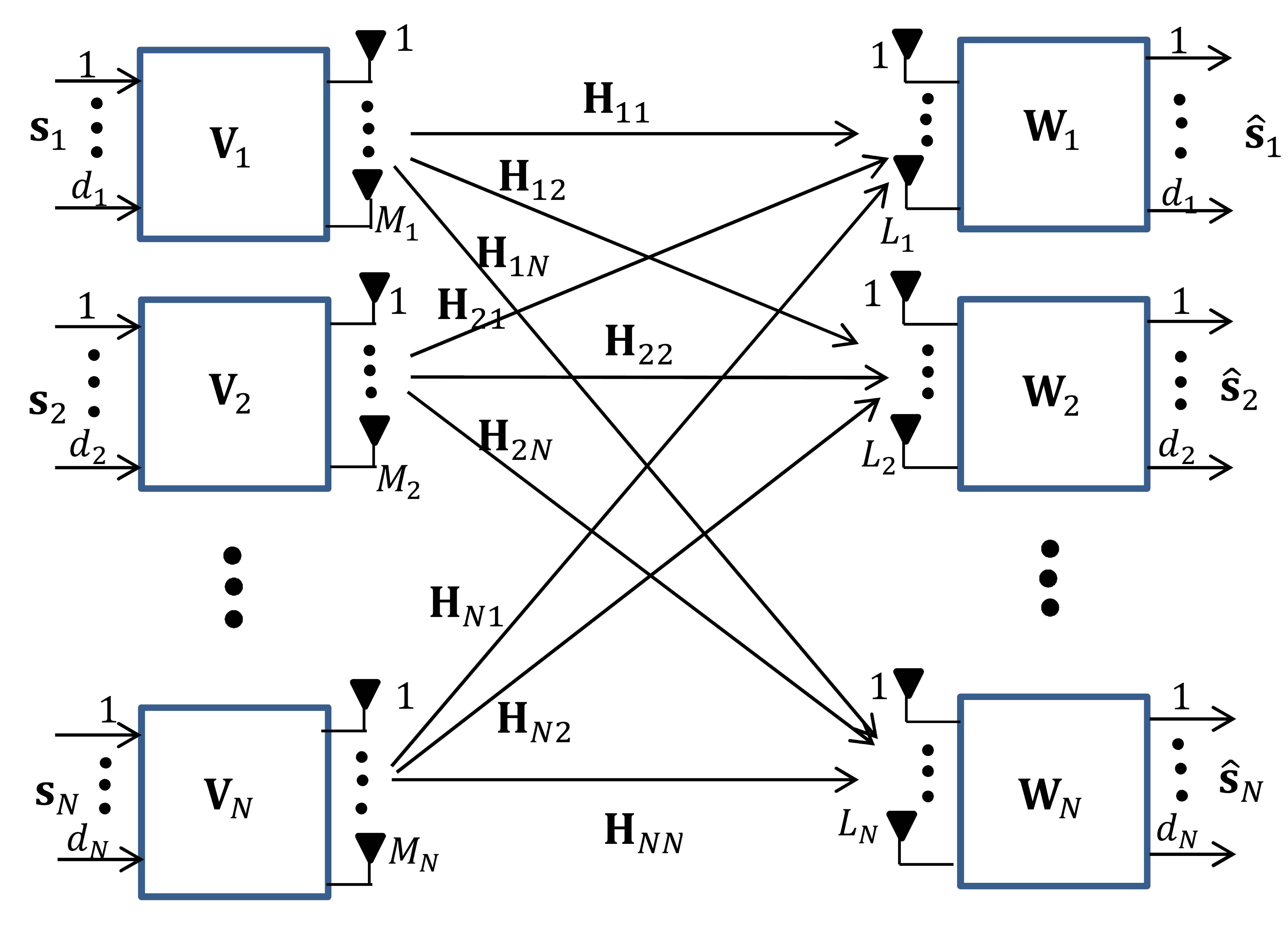
Figure 1: A generic MIMO-IC.

II System model and Problem formulation

Consider $N$ transmit-receive pairs communicating over a MIMO interference channel as shown in Fig. 1. We assume that the $i$th transmitter and the $j$th receiver are equipped with $M_{i}$ and $L_{j}$ antennas, respectively. The $i$th transmitter uses the linear precoder matrix ${\bf V}_{i}\in{\mathbb{C}}^{M_{i}\times d_{i}}$ to convert the symbol stream ${\bf s}_{i}\in{\mathbb{C}}^{d_{i}\times 1}$ (consisting of $d_{i}$ independent data symbols) into the vector ${\bf d}_{i}\in{\mathbb{C}}^{M_{i}\times 1}$, i.e.,

$${\bf d}_{i}={\bf V}_{i}{\bf s}_{i}$$ (1)

and sends it over flat fading channels. The received signal at the $i$th receiver is given by:

$${\bf y}_{i}=\underbrace{{\bf H}_{ii}{\bf d}_{i}}_{\textrm{desired signal}}+\underbrace{\sum_{j\neq i}{\bf H}_{ji}{\bf d}_{j}+{\bf n}_{i}}_{\textrm{interference plus noise}}$$ (2)

where ${\bf H}_{ji}\in{\mathbb{C}}^{L_{i}\times M_{j}}$ denotes the channel matrix between the $j$th transmitter and the $i$th receiver. Also, ${\bf n}_{i}\in{\mathbb{C}}^{L_{i}\times 1}$ is the circularly symmetric complex Gaussian (CSCG) noise at the $i$th receiver with zero mean and covariance matrix ${\bf\Gamma}_{i}\in{\mathbb{S}}^{++}_{L_{i}}$. The $i$th receiver uses the linear decoder matrix ${\bf W}_{i}\in{\mathbb{C}}^{d_{i}\times L_{i}}$ to obtain $\hat{{\bf s}}_{i}\in{\mathbb{C}}^{d_{i}\times 1}$ which is an estimate of the transmitted vector ${\bf s}_{i}$:

$$\hat{{\bf s}}_{i}= {\bf W}_{i}{\bf y}_{i}$$ (3)

$$= {\bf W}_{i}{\bf H}_{ii}{\bf V}_{i}{\bf s}_{i}+{\bf W}_{i}\sum_{j\neq i}{\bf H}_{ji}{\bf V}_{j}{\bf s}_{j}+{\bf W}_{i}{\bf n}_{i}$$

Assuming the symbol stream ${\bf s}_{i}$ is a Gaussian random vector with zero mean and covariance matrix ${\bf I}_{d_{i}}$, the rate of the $i$th user is given by [negro2010mimo]:

$$R_{i}=\log\det\left({\bf I}_{d_{i}}+{\bf W}_{i}{\bf H}_{ii}{\bf V}_{i}{\bf V}_{i}^{H}{\bf H}_{ii}^{H}{\bf W}_{i}^{H}\left({\bf W}_{i}{\bf C}_{\overline{i}}{\bf W}_{i}^{H}\right)^{-1}\right)$$ (4)

with ${\bf C}_{\overline{i}}$ being the interference plus noise covariance matrix defined as

$${\bf C}_{\overline{i}}={\bf\Gamma}_{i}+\sum_{j\neq i}{\bf H}_{ji}{\bf V}_{j}{\bf V}_{j}^{H}{\bf H}_{ji}^{H}$$ (5)

Employing the conventional LMMSE decoder at the receivers means that the $i$th decoder matrix is given by

$${\bf W}_{i}^{\textrm{LMMSE}}={\bf V}_{i}^{H}{\bf H}_{ii}^{H}\left(\sum_{j=1}^{N}{\bf H}_{ji}{\bf V}_{j}{\bf V}_{j}^{H}{\bf H}_{ji}^{H}+{\bf\Gamma}_{i}\right)^{-1}$$ (6)

By substituting (6) into (4), it can be verified that (for completeness we include a proof of (6) and (7) in Appendix A):

$$R_{i}=\log\det\!\left(\!\!{\bf I}_{d_{i}}+{\bf V}_{i}^{H}{\bf H}_{ii}^{H}\!\left[{\bf\Gamma}_{i}+\sum_{j\neq i}{\bf H}_{ji}{\bf V}_{j}{\bf V}_{j}^{H}{\bf H}_{ji}^{H}\right]^{-1}\!\!\!\!{\bf H}_{ii}{\bf V}_{i}\!\!\right)$$ (7)

Remark 1.

The system model and the proposed design methodology in this paper can be extended to the MIMO interference broadcast channel (MIMO-IBC) (see Appendix B for details on the MIMO-IBC case).

Remark 2.

Interestingly, using the decoder ${{\bf W}}_{i}^{\prime}={\bf V}_{i}^{H}{\bf H}_{ii}^{H}{\bf C}_{\overline{i}}^{-1}$, see (5), leads to the same rate as the LMMSE, see (7). Furthermore, the matrix ${{\bf W}}_{i}^{\prime}$ maximizes the rate in (4). To see this, use standard properties of Schur complement to verify that the inequality

$${\bf V}_{i}^{H}{\bf H}_{ii}^{H}{\bf W}_{i}^{H}({\bf W}_{i}{\bf C}_{\overline{i}}{\bf W}^{H})^{-1}{\bf W}_{i}{\bf H}_{ii}{\bf V}_{i}\preceq{\bf V}_{i}^{H}{\bf H}_{ii}^{H}{\bf C}_{\overline{i}}^{-1}{\bf H}_{ii}{\bf V}_{i}$$ (8)

is equivalent to the positive semi-definitness of the matrix:

$${\bf\Phi}_{i}=\left[\begin{array}[]{cc}{\bf V}_{i}^{H}{\bf H}_{ii}^{H}{\bf C}_{\overline{i}}^{-1}{\bf H}_{ii}{\bf V}_{i}&{\bf V}_{i}^{H}{\bf H}_{ii}^{H}{\bf W}_{i}^{H}\\ {\bf W}_{i}{\bf H}_{ii}{\bf V}_{i}&{\bf W}_{i}{\bf C}_{\overline{i}}{\bf W}^{H}\\ \end{array}\right].$$ (9)

Now, observe that the matrix ${\bf\Phi}_{i}$ above indeed is in ${\mathbb{S}}^{+}_{d_{i}}$ because it can be decomposed as ${\bf\Phi}_{i}={\bm{\Theta}}_{i}{\bm{\Theta}}_{i}^{H}$ with

$${\bm{\Theta}}_{i}=\left[\begin{array}[]{cc}{\bf V}_{i}^{H}{\bf H}_{ii}^{H}&{\bm{0}}\\ {\bm{0}}&{\bf W}_{i}\\ \end{array}\right]\left[\begin{array}[]{cc}{\bf C}_{\overline{i}}^{-1/2}\\ {\bf C}_{\overline{i}}^{1/2}\\ \end{array}\right]$$ (10)

Therefore, (8) holds true. Moreover, it can be verified that by substituting ${\bf W}_{i}={\bf W}_{i}^{\prime}={\bf V}_{i}^{H}{\bf H}_{ii}^{H}{\bf C}_{\overline{i}}^{-1}$ in (8), the left-hand side becomes ${\bf V}_{i}^{H}{\bf H}_{ii}^{H}{\bf C}_{\overline{i}}^{-1}{\bf H}_{ii}{\bf V}_{i}$ which is equal to the right-hand side. Therefore, ${\bf W}_{i}^{\prime}$ maximizes the rate in (4). Because the LMMSE decoder in (6) and ${\bf W}_{i}^{\prime}$ yield the same rate, we conclude that the LMMSE decoder maximizes the rate as well. Note that the optimality of this decoder for mean square error minimization has been addressed in [5756489, razaviyayn2013linear] (see also [schmidt2009minimum]). $\blacksquare$

Using Sylvester’s determinant property, i.e. $\det({\bf I}+{\bf A}{\bf B})=\det({\bf I}+{\bf B}{\bf A})$, the rate $R_{i}$ in (7) can be rewritten as

$$R_{i}=\log\det\!\left({\bf I}_{L_{i}}+{\bf H}_{ii}{\bf Q}_{i}{\bf H}_{ii}^{H}\!\left[{\bf\Gamma}_{i}+\sum_{j\neq i}{\bf H}_{ji}{\bf Q}_{j}{\bf H}_{ji}^{H}\right]^{-1}\right)$$ (11)

where ${\bf Q}_{i}\triangleq{\bf V}_{i}{\bf V}_{i}^{H}\in{\mathbb{C}}^{M_{i}\times M_{i}},i=1,\dots,N$, are the precoder covariance matrices. In this paper, the goal is to design the precoder covariance matrices $\{{\bf Q}_{i}\}_{i=1}^{N}$ to maximize the minimum rate of the users, which can be cast as the following problem:

$$\!\max_{\{{\bf Q}_{i}\}_{{i=1}}^{N}}\,\min_{i=1,2,\dots,N}\quad {R_{i}}$$ (12)

s.t. $$\operatorname{tr}\{{\bf Q}_{i}\}\leq p_{i}\qquad \forall i=1,2,\dots,N$$

$${\bf Q}_{i}\succeq\textbf{0}\qquad \forall i=1,2,\dots,N$$

where $p_{i}$ is the power available to the $i$th transmitter. Note that in the covariance design approach, we jointly design the optimum precoder matrices $\{{\bf V}_{i}\}_{i=1}^{N}$, as well as, the optimum number of their columns $\{d_{i}\}_{i=1}^{N}$, i.e. the length of symbol streams. More precisely, we fully exploit the available degrees of freedom of the design problem instead of considering the design problem in a limited framework in which $\{d_{i}\}_{i=1}^{N}$ are assumed to be a priori known.

In the next section, we assume that the noise covariance matrices ${\{{\bf\Gamma}_{i}\}}_{i=1}^{N}$ as well as the channel matrices $\{{\bf H}_{ij}\}_{{i,j=1}}^{N}$ are exactly known. We consider the case of uncertain a priori knowledge in Section IV.

III the proposed method

III-A Derivation of the proposed method

It can be shown that the design problem in (12) is non-convex and NP-hard in general [razaviyayn2013linear]. In what follows we devise a method based on the minorization-maximization (MM) technique [stoica2004cyclic] to tackle this problem.

In (12) the constraints are convex but the objective function is non-convex. Therefore we will apply the MM technique to the objective function. For this purpose, we first introduce the following proposition.

Proposition 1.

The rate $R_{i}$, see (11), can be rewritten as:

$$R_{i}=\log\det({\bf U}^{H}{\bf B}_{i}^{-1}{\bf U})$$ (13)

where ${\bf U}$ and ${\bf B}_{i}$ are defined as,

$${\bf U}\triangleq\left[\begin{array}[]{cc}{\bf I}_{M_{i}}&\textbf{0}_{M_{i}\times L_{i}}\\ \end{array}\right]^{T}$$ (14)

and

$${\bf B}_{i}=\left[\begin{array}[]{cc}{\bf I}_{M_{i}}&\widetilde{{\bf V}}^{H}_{i}{\bf H}_{ii}^{H}\\ {\bf H}_{ii}\widetilde{{\bf V}}_{i}&{\bf\Gamma}_{i}+\displaystyle\sum_{j=1}^{N}{\bf H}_{ji}\widetilde{{\bf V}}_{j}\widetilde{{\bf V}}_{j}^{H}{\bf H}_{ji}^{H}\\ \end{array}\right]$$ (15)

with $\widetilde{{\bf V}}_{i}\triangleq{\bf Q}_{i}^{\frac{1}{2}}\in{\mathbb{C}}^{M_{i}\times M_{i}}$.

Proof:

See Appendix C. $\blacksquare$

By using (13), the problem in (12) can be rewritten as follows

$$\max_{\{\widetilde{{\bf V}}_{i}\}_{{i=1}}^{N},} \min_{i=1,\cdots,N}\log\det({\bf U}^{H}{\bf B}_{i}^{-1}{\bf U})\$$ (16)

s.t. $$\operatorname{tr}\{\widetilde{{\bf V}}_{i}\widetilde{{\bf V}}_{i}^{H}\}\,\leq\,p_{i},\,\,\,\forall i=1,2,\dots,N$$

The following lemma (see, e.g., [naghsh]) lays the ground for applying MM to (16).

TABLE II: The proposed method for the max-min rate design of the transmit covariance matrices in MIMO-IC.

Step 1: Initialize $\{{\bf x}_{i}\}_{i=1}^{N}$ with complex random vectors in ${\mathbb{C}}^{M_{i}^{2}\times 1}$ such that they satisfy $\|{\bf x}_{i}\|_{2}^{2}\leq p_{i}$.

Step 2: Solve the (convex) SOCP problem in (LABEL:pzegon).

Step 3: Update ${\bf b}_{i}$, ${\bf G}_{ji}$, and $C_{i}$ according to equations (LABEL:F), (LABEL:gb), (LABEL:gb1), and (LABEL:ci), respectively.

Step 4: Repeat steps 1 and 2 until a pre-defined stop criterion is satisfied, e.g $|t^{(\kappa)}-t^{(\kappa-1)}|\leq\epsilon$, for a given $\epsilon>0$.

IV Precoder Design in the presence of a priori knowledge uncertainty

In practice there always exist uncertainties in the noise covariance and the channel state information. In this section we will consider these uncertainties in the design problem.

We first consider the effect of imperfect CSI due to channel estimation errors. Using the conventional LMMSE estimator, the channels can be modeled as [kay1993fundamentals]:

$${\bf H}_{ji}=\hat{{\bf H}}_{ji}+{\bf Z}_{ji}$$ (39)

where $\hat{{\bf H}}_{ji}$ is the estimate of the true channel ${{\bf H}}_{ji}$ and ${\bf Z}_{ji}$ is the channel estimation error which is assumed to be uncorrelated with $\hat{{\bf H}}_{ji}$. Assuming the entries of ${\bf H}_{ji}$ are i.i.d random variables (RVs) with variances $\sigma^{2}_{ji}$, the entries of $\hat{{\bf H}}_{ji}$ and ${\bf Z}_{ji}$ will be i.i.d RVs with variances $\rho_{ji}^{2}\sigma^{2}_{ji}$ and $(1-\rho_{ji}^{2})\sigma^{2}_{ji}$, respectively. The parameter $\rho_{ji}\in[0,1]$ quantifies the estimation accuracy, in particular if $\rho_{ji}=1$, $\hat{{\bf H}}_{ji}={{\bf H}}_{ji}$ and CSI is perfect.

Substituting (39) in (2), we obtain:

$${\bf y}_{i}=\underbrace{\hat{{\bf H}}_{ii}{{\bf V}^{\prime}}_{i}{\bf s}_{i}}_{\textrm{desired signal}}+\underbrace{\sum_{j\neq i}\hat{{\bf H}}_{ji}{{\bf V}^{\prime}}_{j}{\bf s}_{j}+\sum_{j=1}^{N}{{\bf Z}}_{ji}{{\bf V}^{\prime}}_{j}{\bf s}_{j}+{\bf n}_{i}}_{\textrm{interference plus estimation error and noise}}$$ (40)

with ${{\bf V}^{\prime}}_{i}$ being the precoder matrix of the $i$th transmitter designed under imperfect CSI. It can be proved that:

$$\mathbb{E}\left\{{{\bf Z}}_{ji}{{\bf V}^{\prime}}_{j}{{\bf V}^{\prime}}_{j}^{H}{{\bf Z}}_{ji}^{H}\right\}=(1-\rho_{ji}^{2})\sigma^{2}_{ji}\operatorname{tr}\{{{\bf V}^{\prime}}_{j}{{\bf V}^{\prime}}_{j}^{H}\}{\bf I}_{L_{i}}$$ (41)

Therefore, the LMMSE decoder will be:

$$\hat{{\bf W}}_{i}^{\textrm{LMMSE}}= {{\bf V}^{\prime}}_{i}^{H}\hat{{\bf H}}_{ii}^{H}\left(\sum_{j=1}^{N}\hat{{\bf H}}_{ji}{{\bf V}^{\prime}}_{j}{{\bf V}^{\prime}}_{j}^{H}\hat{{\bf H}}_{ji}^{H}+\right.$$ (42)

$$\left.\sum_{j=1}^{N}(1-\rho_{ji}^{2})\sigma^{2}_{ji}\operatorname{tr}\{{{\bf V}^{\prime}}_{j}{{\bf V}^{\prime}}_{j}^{H}\}{\bf I}_{L_{i}}+{\bf\Gamma}_{i}\right)^{-1}$$

Let ${{\bf Q}^{\prime}}_{j}\triangleq{{\bf V}^{\prime}}_{j}{{\bf V}^{\prime}}_{j}^{H}$ be the precoder covariance matrices in the imperfect CSI case. Note that the term $\sum_{j=1}^{N}{{\bf Z}}_{ji}{{\bf V}^{\prime}}_{j}{\bf s}_{j}$ in (40) is the sum of the products of Gaussian random variables (i.e. ${\bf Z}_{ji}$ and ${\bf s}_{j}$) and hence, it is no longer Gaussian; this observation leads to difficulties for computation of the user rate. Therefore, in this case, we resort to a common approach in the literature (see e.g. [wang2012efficient, ngo2013energy, ho2011decentralized] and references therein) to make the problem tractable; more precisely, the following lower bound $\hat{R}_{i}$ on the rate of the $i$th user is considered as the design metric:

$${\hat{R}}_{i}=\log\det\! \left({\bf I}_{L_{i}}+\hat{{\bf H}}_{ii}{{\bf Q}^{\prime}}_{i}\hat{{\bf H}}_{ii}^{H}\!\left[{\bf\Gamma}_{i}+\sum_{j\neq i}\hat{{\bf H}}_{ji}{{\bf Q}^{\prime}}_{j}\hat{{\bf H}}_{ji}^{H}\right.\right.$$ (43)

$$\left.\left.+\sum_{j=1}^{N}(1-\rho_{ji}^{2})\sigma^{2}_{ji}\operatorname{tr}\{{\bf Q}^{\prime}_{j}\}{\bf I}_{L_{j}}\right]^{-1}\right)$$

Next, we also consider the uncertainty of the noise covariance matrices, which can be modeled as [naghsh]:

$$\|{\bf\Gamma}_{i}-\hat{{\bf\Gamma}}_{i}\|_{2}\leq\zeta_{i},\quad\forall i=1,\cdots,N$$ (44)

where $\hat{{\bf\Gamma}}_{i}$s are known positive definite matrices (initial guesses of the covariance matrices) and $\zeta_{i}$s are positive scalars that determine the size of the uncertainty regions. We remark on the fact that in the case of imperfect CSI, we have uncertainty about the true channel value; however, in the case of noise vectors, we consider uncertainty in the noise covariance matrix (rather than in the noise vector). Therefore, we consider a worst-case approach to deal with uncertain noise covariance matrices which is commonly used in literature (see for instance [karbasi2015knowledge, dong2006finite]).

We can robustify the design method with respect to a priori knowledge uncertainty by considering the following reformulation of the optimization problem:

$$\!\max_{\{{{\bf Q}^{\prime}}_{i}\}_{{i=1}}^{N}}\, \min_{i=1,\dots,N}\min_{\{{{\bf\Gamma}_{i}}\}_{{i=1}}^{N}}\quad{\hat{R}_{i}}$$ (45)

s.t. $$\operatorname{tr}\{{{\bf Q}^{\prime}_{i}}\}\,\leq\,p_{i},\quad \forall i=1,2,\dots,N$$

$$\|{\bf\Gamma}_{i}-\hat{{\bf\Gamma}}_{i}\|_{2}\leq\zeta_{i},\quad \forall i=1,2,\cdots,N$$

$${\bf\Gamma}_{i}\succeq\textbf{0},{{\bf Q}^{\prime}_{i}}\succeq\textbf{0}\quad \forall i=1,2,\cdots,N$$

where ${\hat{R}}_{i}$ is as given in (43). In what follows we present a theorem which shows that the problem in (45) can be dealt with via a modified version of the method proposed in Section III.