Excitation of bound states in the continuum via second harmonic generations

Abstract

A bound state in the continuum (BIC) on a periodic structure sandwiched between two homogeneous media is a guided mode with a frequency and a wavenumber such that propagating plane waves with the same frequency and wavenumber exist in the homogeneous media. Optical BICs are of significant current interest, since they have applications in lasing, sensing, filtering, switching, and many light emission processes, but they cannot be excited by incident plane waves when the structure consists of linear materials. In this paper, we study the diffraction of a plane wave by a periodic structure with a second order nonlinearity, assuming the structure has a BIC and the frequency and wavenumber of the incident wave are one half of those of the BIC. Based on a scaling analysis and a perturbation theory, we show that the incident wave may induce a very strong second harmonic wave dominated by the BIC, and also a fourth harmonic wave that cannot be ignored. The perturbation theory reveals that the amplitude of the BIC is inversely proportional to a small parameter depending on the amplitude of the incident wave and the nonlinear coefficient. In addition, a system of four nonlinearly coupled Helmholtz equations (the four-wave model) is proposed to model the nonlinear process. Numerical solutions of the four-wave model are presented for a periodic array of circular cylinders and used to validate the perturbation results.

35Q60, 78A45, 78A60

1 Introduction

The concept of bound state in the continuum (BIC) was originally introduced by von Neumann and Wigner for a quantum system [1]. For classical waves, a BIC is a trapped or guided mode on a structure with a frequency at which radiative waves carrying power to or from infinity also exist. Mathematically, a BIC corresponds to an eigenvalue in the continuous spectrum. At the frequency of the BIC, boundary value problems for given incident waves from infinity have no uniqueness [2]. BICs have been studied for sound waves, linear water waves, and electromagnetic waves (including light) based on Helmholtz and Maxwell’s equations. They exist on different kind of structures including waveguides with local distortions [3], waveguides with lateral leaky channels [4], and periodic structures sandwiched between two homogeneous media [2, 5, 6, 7, 8, 9, 10, 11, 12, 13]. Some BICs exist because they have a symmetry mismatch with radiative waves, and they are often regarded as symmetry-protected [2, 3, 4, 5, 6, 8, 12]. Other BICs seem to decouple with the radiative waves accidentally [14]. On periodic structures sandwiched between two homogeneous media, there could be BICs that propagate along the periodic directions [6, 7, 9, 10, 11, 13]. These BICs are not protected by symmetry in the usual sense, but in some cases, they depend strongly on the symmetry [15, 16]. Unlike the well-known guided modes, a propagating BIC on a periodic structure exists above the lightline, that is, it co-exists with plane waves in the homogeneous media for the same frequency and a compatible wavevector. Recently, BICs have attracted much attention in optics due to their interesting properties and potential applications [17]. Since the BICs are decoupled from the radiative waves, they cannot be excited by incident waves coming from infinity. Bulgakov et al. [18] suggested to use the nonlinear optical Kerr effect [19] to excite the BICs. However, with the Kerr effect, the BICs become nonlinear [20] and the associated diffraction problem exhibits complicated optical bistability and symmetry-breaking phenomena [21, 22].

In this paper, we study the excitation of BICs based on a second order nonlinear process [19]. The second order nonlinearity gives quadratic nonlinear terms in the Maxwell’s equations, and it is responsible for the second harmonic generation (SHG) process, i.e, waves with frequency $2\omega$ are generated when the incident wave is of frequency $\omega$. SHG is the first nonlinear process studied in the field of nonlinear optics [23]. Most existing studies on SHG aim to increase the percentage of power converted from the incident wave to the second harmonic wave [19]. Mathematical problems associated with SHG have been studied more than two decades ago [24, 25, 26]. Our objective is different. We aim to generate a wave field which is dominated by a BIC. To excite a BIC on a periodic structure with frequency $\omega_{*}$, we illuminate the structure with an incident wave of fundamental frequency $\omega=\omega_{*}/2$. A second harmonic field (of frequency $2\omega=\omega_{*}$) is generated due to the second order nonlinearity. Part of that second harmonic field is proportional to the BIC which does not leak out power. Our objective is to determine the amplitude of that BIC. Using a perturbation method, we show that the amplitude of the BIC is proportional to $A/\delta$, where $A$ is the amplitude of the incident wave, $\delta=\sqrt[3]{A\gamma_{1}}$ is a dimensionless small parameter, and $\gamma_{1}$ is the magnitude of a nonlinear coefficient (one element of the second order nonlinear susceptibility tensor). In addition, we show that the fourth harmonic wave (with frequency $2\omega_{*}$) cannot be ignored. The amplitude of the BIC can only be corrected determined when the fourth harmonic is included in a coupled system. Therefore, the BIC generation process is very different from the standard SHG process. To validate the theoretical results, we present numerical results for a periodic array of nonlinear circular cylinders.

The rest of this paper is organized as follows. In section 2, the governing equations, simplified models and boundary conditions are derived for two-dimensional (2D) structures and the $E$ polarization. A perturbation theory including a formula for the coefficient of the BIC is developed in section 3. Numerical methods for solving a nonlinear model with four frequencies are presented in section 4. Numerical solutions of the nonlinear model are compared with the perturbation results in section 5. The paper is concluded with some remarks in section 6.

2 Problem formulation

We consider a 2D lossless nonlinear non-dispersive periodic structure which is invariant in the $z$ direction, periodic in the $y$ direction with period $L$, and sandwiched between two identical linear homogeneous media (given in $x<-D$ and $x>D$ respectively for a positive constant $D$). The structure is described by a real dielectric function $\epsilon=\epsilon(x,y)$ and a real second order nonlinear susceptibility tensor [19], both of which are periodic in $y$ with period $L$. In addition, $\epsilon(x,y)=\epsilon_{0}>0$ and the nonlinear susceptibility tensor is zero for $|x|>D$. For the $E$ polarization, the electromagnetic fields are independent of $z$ and the only nonzero component of the electric field is its $z$ component, denoted as $E_{z}$. In that case, the time-domain Maxwell’s equations with a second order nonlinearity can be reduced to the following scalar equation [19]

(1) $$\frac{\partial^{2}E_{z}}{\partial x^{2}}+\frac{\partial^{2}E_{z}}{\partial y^{2}}-\frac{\epsilon}{c^{2}}\frac{\partial^{2}E_{z}}{\partial t^{2}}-\frac{\gamma}{c^{2}}\frac{\partial^{2}E^{2}_{z}}{\partial t^{2}}=0,$$

where $c$ is the speed of the light in vacuum and $\gamma=\gamma(x,y)$ is one element of the second order nonlinear susceptibility tensor.

For an incident wave with frequency $\omega$ (fundamental frequency), we can expand the wave field in harmonic waves as

(2) $$E_{z}=\mbox{Re}\left(u_{1}e^{-i\omega t}+u_{2}e^{-2i\omega t}+u_{3}e^{-3i\omega t}+u_{4}e^{-4i\omega t}+\ldots\right),$$

where $u_{1}=u_{1}(x,y)$ is the complex amplitude of the fundamental frequency wave, and $u_{n}=u_{n}(x,y)$ ($n>1$) is the complex amplitude of the $n$-th order harmonic wave. Substituting Eq. (2) into Eq. (1), we obtain the following infinite coupled system of nonlinear equations:

(3) $${\cal L}_{n}u_{n}=-\frac{n^{2}k^{2}}{2}\gamma\left(\sum_{m=1}^{n}u_{m}u_{n-m}+2\sum_{m=1}^{\infty}\bar{u}_{m}u_{m+n}\right),$$

where $u_{0}\equiv 0$, $k=\omega/c$, and

(4) $${\cal L}_{n}=\frac{\partial^{2}}{\partial x^{2}}+\frac{\partial^{2}}{\partial y^{2}}+n^{2}k^{2}\epsilon.$$

The incident wave is assumed to be a plane wave given in the left linear homogeneous medium:

(5) $$u^{(i)}_{1}(x,y)=Ae^{i(\alpha x+\beta y)},\quad x<-D,$$

where $A$ is the amplitude, $(\alpha,\beta)$ is a real wave vector, $\alpha>0$ and $\alpha^{2}+\beta^{2}=k^{2}\epsilon_{0}$.

In practice, to solve the nonlinear diffraction problem associated with the above incident wave, one has to truncate the infinite coupled system to a finite system. In standard theories on SHG [24, 25, 26], high order harmonic waves are weak, and it is sufficient to keep the fundamental frequency and second harmonic waves. Thus, the infinite system is approximated by

(6) $${\cal L}_{1}u_{1} = -k^{2}\gamma\bar{u}_{1}u_{2},$$

(7) $${\cal L}_{2}u_{2} = -2k^{2}\gamma u_{1}^{2}.$$

We refer the above system, (6)-(7), as the two-wave model. For many cases, the second harmonic wave is much weaker than the fundamental frequency wave, so the nonlinear coupling term in the right hand side of Eq. (6) can be ignored. In that case, $u_{1}$ satisfies a linear homogeneous Helmholtz equation and is unaffected by $u_{2}$, and $u_{2}$ satisfies a linear inhomogeneous Helmholtz equation with $u_{1}^{2}$ in the right hand side of Eq. (7) as a source term. This is the so-called un-depleted pump approximation.

We are interested in the case where the linear periodic structure (with the same dielectric function $\epsilon$ and a zero nonlinear susceptibility tensor) has a BIC $u_{*}$ with frequency $\omega_{*}$. The BIC satisfies the linear Helmholtz equation

(8) $$\frac{\partial^{2}u_{*}}{\partial x^{2}}+\frac{\partial^{2}u_{*}}{\partial y^{2}}+k_{*}^{2}\epsilon u_{*}=0,$$

where $k_{*}=\omega_{*}/c$ and $u_{*}$ decays to zero exponentially as $|x|\to\infty$. Since the structure is periodic in $y$, the BIC is a Bloch mode given as

(9) $$u_{*}(x,y)=e^{i\beta_{*}y}\phi_{*}(x,y),$$

where $\beta_{*}\in[-\pi/L,\pi/L]$ is the real Bloch wavenumber, and $\phi_{*}$ is periodic in $y$ with period $L$. Importantly, the BIC is above the lightline, that is,

(10) $$k_{*}>|\beta_{*}|/\sqrt{\epsilon_{0}}.$$

The above condition implies that $\alpha_{*}=\sqrt{k_{*}^{2}\epsilon_{0}-\beta_{*}^{2}}$ is real and the plane waves $e^{i(\beta_{*}y\pm\alpha_{*}x)}$ can propagate to or from infinity in the surrounding linear media with dielectric constant $\epsilon_{0}$. In order to excite the BIC by the second order nonlinear effect, we specify the frequency and wavevector of the incident wave given in Eq. (5) by

(11) $$\omega=\frac{\omega_{*}}{2},\quad\beta=\frac{\beta_{*}}{2},\quad\alpha=\frac{\alpha_{*}}{2}.$$

Since the nonlinear coefficient $\gamma$ is very small for ordinary nonlinear optical materials, and the incident wave is normally not extremely strong, we are interested in the regime for which the dimensionless quantity $A\gamma_{1}$ is small, where $\gamma_{1}=\max|\gamma(x,y)|$ is magnitude of $\gamma$. In normal circumstances, this assumption implies that the third and higher harmonics can be ignored and the two-wave model is accurate. Our case is different, since the second harmonic wave contains a BIC which does not lose power to infinity and there is no material dissipation. If we consider an initial value problem by turning on the incident wave at $t=0$, then the amplitude of the BIC in the second harmonic wave is expected to increase with time. However, this amplitude can only approach a finite limit as $t\to\infty$, since when the second harmonic wave is sufficiently strong, its own SHG (generation of fourth harmonic wave from the second harmonic wave) becomes important. In section 3, we show that it is necessary to keep the fourth harmonic wave in the system. This leads to the following three-wave model:

(12) $${\cal L}_{1}u_{1} = -k^{2}\gamma\bar{u}_{1}u_{2},$$

(13) $${\cal L}_{2}u_{2} = -2k^{2}\gamma(u_{1}^{2}+2\bar{u}_{2}u_{4}),$$

(14) $${\cal L}_{4}u_{4} = -8k^{2}\gamma u_{2}^{2}.$$

We can also keep $u_{3}$ and use the following four-wave model:

(15) $${\cal L}_{1}u_{1} = -k^{2}\gamma\left(\bar{u}_{1}u_{2}+\bar{u}_{2}u_{3}+\bar{u}_{3}u_{4}\right),$$

(16) $${\cal L}_{2}u_{2} = -2k^{2}\gamma\left(u_{1}^{2}+2\bar{u}_{1}u_{3}+2\bar{u}_{2}u_{4}\right),$$

(17) $${\cal L}_{3}u_{3} = -9k^{2}\gamma\left(u_{1}u_{2}+\bar{u}_{1}u_{4}\right),$$

(18) $${\cal L}_{4}u_{4} = -8k^{2}\gamma\left(u_{2}^{2}+2u_{1}u_{3}\right).$$

Since the medium for $|x|>D$ is linear, i.e., $\gamma(x,y)=0$ for $|x|>D$, the equations for $u_{n}$, both the exact Eq. (3) and the approximate ones in the three- or four-wave models, are reduced to linear homogeneous Helmholtz equations for $|x|>D$. Therefore, we can set up transparent boundary conditions at $x=\pm D$ following the standard practice [27, 28]. More precisely, for integer $n\geq 1$, we let

(19) $$\beta^{(n)}_{m}=n\beta+\frac{2m\pi}{L},\quad\alpha^{(n)}_{m}=\left[n^{2}k^{2}\epsilon_{0}-(\beta^{(n)}_{m})^{2}\right]^{1/2}$$

for all integers $m$, define a linear operator $\mathcal{T}_{n}$ such that

(20) $$\mathcal{T}_{n}e^{i\beta^{(n)}_{m}y}=i\alpha^{(n)}_{m}e^{i\beta^{(n)}_{m}y},\quad\mbox{for}\quad m=0,\pm 1,\pm 2,\ldots,$$

then the boundary conditions are

(21) $$\frac{\partial u_{n}}{\partial x}=\mathcal{T}_{n}u_{n},\quad x=D,\quad n\geq 1,$$

(22) $$\frac{\partial u_{n}}{\partial x}=-\mathcal{T}_{n}u_{n},\quad x=-D,\quad n\geq 2.$$

Notice that Eq. (22) is not valid for $n=1$. Since there is an incident wave of frequency $\omega$ given in the left homogeneous medium, the boundary condition of $u_{1}$ at $x=-D$ should be

(23) $$\frac{\partial u_{1}}{\partial x}=-\mathcal{T}_{1}u_{1}+2iA\alpha e^{i\beta y},\quad x=-D.$$

Moreover, since the structure is periodic in $y$, all harmonic waves are quasi-periodic in $y$, i.e.,

(24) $$u_{n}(x,L/2)=e^{in\beta L}u_{n}(x,-L/2),$$

(25) $$\partial_{y}u_{n}(x,L/2)=e^{in\beta L}\partial_{y}u_{n}(x,-L/2).$$

With boundary conditions (21)-(25), we can solve the truncated nonlinear systems, such as the the four-wave model, in the following rectangular domain

(26) $$\Omega=\left\{(x,y)\ |\ -D<x<D,\ -L/2<y<L/2\right\}.$$

Assuming the nonlinear coefficient $\gamma$ is real, then the two-, three- and four-wave models are all energy conserving, in the sense that the power carried by the incident wave equals the total power radiated out by the fundamental frequency wave and the retained harmonic waves. For $n\geq 2$, the power per period radiated out by $u_{n}$ can be calculated by integrating the $x$ component of the complex Poynting vector at $x=\pm D$ with respect to $y$, and up to a constant scaling, it is

(27) $$P_{n}^{\rm out}=\frac{1}{2nk}\int_{-L/2}^{L/2}\mbox{Im}\left[\overline{u}_{n}\frac{\partial u_{n}}{\partial x}\right]_{x=-D}^{x=D}dy.$$

The power (per period) carried by the incident wave is

(28) $$P_{1}^{\rm inc}=\frac{1}{2k}\int_{-L/2}^{L/2}\mbox{Im}\left[\overline{u}^{(i)}_{1}\frac{\partial u_{1}^{(i)}}{\partial x}\right]_{x=-D}dy=\frac{\alpha L|A|^{2}}{2k}.$$

For $u_{1}$, we have a reflected wave $u_{1}^{(r)}$ and a transmitted wave $u_{1}^{(t)}$ satisfying $u_{1}=u_{1}^{(i)}+u_{1}^{(r)}$ for $x<-D$ and $u_{1}=u_{1}^{(t)}$ for $x>D$. Thus, the power radiated out by the fundamental frequency wave is

(29) $$P_{1}^{\rm out}=\frac{1}{2k}\int_{-L/2}^{L/2}\mbox{Im}\left\{\left[\overline{u}_{1}^{(t)}\frac{\partial u_{1}^{(t)}}{\partial x}\right]_{x=D}-\left[\overline{u}_{1}^{(r)}\frac{\partial u_{1}^{(r)}}{\partial x}\right]_{x=-D}\right\}dy.$$

The energy conservation property of the four-wave model is

(30) $$P_{1}^{\rm inc}=\sum_{n=1}^{4}P_{n}^{\rm out}.$$

To show this, we realize that

$$\sum_{n=1}^{4}\frac{1}{n}\int_{\Omega}\overline{u}_{n}{\cal L}_{n}u_{n}dxdy=-2k^{2}\int_{\Omega}\gamma\mbox{Re}\left(\overline{u}_{1}^{2}u_{2}+3\overline{u}_{1}\overline{u}_{2}u_{3}+4\overline{u}_{1}\overline{u}_{3}u_{4}+2\overline{u}_{2}^{2}u_{4}\right)dxdy$$

is real. Thus, the imaginary part of the left hand side above is zero, and it can be written as

(31) $$\sum_{n=1}^{4}\frac{1}{n}\int_{-L/2}^{L/2}\mbox{Im}\left[\overline{u}_{n}\frac{\partial u_{n}}{\partial x}\right]_{x=-D}^{x=D}dy=0.$$

After verifying the term for $n=1$ in the left hand side above is actually $2k(P_{1}^{\rm out}-P_{1}^{\rm inc})$, Eq. (30) is obtained. The ratio $P_{n}^{\rm out}/P_{1}^{\rm inc}$ (for $n\neq 1$) is referred to as the conversion efficiency for the $n$-th harmonic wave.

3 Perturbation theory

In this section, we first determine the scaling for the first a few harmonic waves from the exact Eq. (3). For $A$ and $\gamma_{1}$ given in section 2, we let $A\gamma_{1}=\delta^{3}$ and assume $\delta$ is small. The cubic for $\delta$ is introduced for convenience. We also assume that the periodic structure supports a single (i.e., non-degenerate) BIC with frequency $\omega_{*}=2\omega$ and Bloch wavenumber $\beta_{*}=2\beta$, and there is no BIC with frequency $n\omega$ and Bloch wavenumber $n\beta$ for $n\neq 2$. Since the incident wave has amplitude $A$, $u_{1}$ should remain at $O(A)$, $u_{3}$ and $u_{4}$ should be smaller, but $u_{2}$ may contain a large term proportional to the BIC, because the power converted to the second harmonic wave can accumulate in the BIC. Note that the equation for $u_{2}$ is singular, and it does not have a solution unless the right hand side is orthogonal to the BIC $u_{*}$. The right hand side of the exact equation, Eq. (3) for $n=2$, contains the terms $u_{1}^{2}$, $\overline{u}_{1}u_{3}$, $\overline{u}_{2}u_{4}$, etc. In general, the orthogonality condition cannot be satisfied by the term $u_{1}^{2}$ alone. Therefore, one other term must have the same order as $u_{1}^{2}$. Since $u_{3}$ is smaller than $u_{1}$ (in magnitude), $\overline{u}_{1}u_{3}$ cannot balance $u_{1}^{2}$. Therefore, $\overline{u}_{2}u_{4}$ should have the same order as $u_{1}^{2}$, that is $\overline{u}_{2}u_{4}=O(A^{2})$. On the other hand, the scaling of $u_{4}$ can be determined from the dominant term in the right hand side of its own equation. The right hand side of Eq. (3) for $n=4$ contains $u_{1}u_{3}$, $u_{2}^{2}$, $\overline{u}_{1}u_{5}$, $\overline{u}_{2}u_{6}$, etc. For consistency, it is necessary to assume that $u_{2}^{2}$ is the dominant term. Therefore, we have $u_{4}=O(\gamma_{1}u_{2}^{2})$. From this and the condition $\overline{u}_{2}u_{4}=O(A^{2})$, it is easy to deduce that $u_{2}=O(A/\delta)$ and $u_{4}=O(A\delta)$. To determine the scaling for $u_{3}$, we consider the right hand side of its equation, conclude that $u_{1}u_{2}$ should be the dominant term, and thus $u_{3}=O(A\delta^{2})$. Similarly, $u_{5}=O(A\delta^{4})$, $u_{6}=O(A\delta^{3})$, etc. Since $u_{4}$ is essential to the equation for $u_{2}$, a minimal truncated system may include $u_{1}$, $u_{2}$ and $u_{4}$ only. This leads to the three-wave model (12)-(14). We prefer to keep $u_{3}$ and use the four-wave model (15)-(18). Some small terms in the right hand sides of the four-wave model are probably not important, because they are on the same order as the terms dropped due to the truncation. For example, the original equation for $u_{4}$ has a term $\overline{u}_{2}u_{6}$ which is $O(A^{2}\delta^{2})$, same as the retained term $u_{1}u_{3}$. In the equation for $u_{3}$, the term $\overline{u}_{1}u_{4}$ is on the same order as the dropped term $\overline{u}_{2}u_{5}$. This suggests that the the four-wave model may be slightly simplified by removing these terms. However, we will not explore these minor simplifications.

Next, we use a perturbation method and the four-wave model to find the leading coefficient of the BIC in the second harmonic wave. Writing the nonlinear coefficient as $\gamma(x,y)=\gamma_{1}F(x,y)$ where $F(x,y)=0$ in the linear media and $\max|F(x,y)|=1$, we expand $u_{1}$, $u_{2}$, $u_{3}$ and $u_{3}$ as

(32) $$u_{1} = A\left(u_{10}+\delta^{2}u_{11}+\dots\right),$$

(33) $$u_{2} = A\left(\delta^{-1}u_{20}+\delta u_{21}+\delta^{3}u_{22}+\dots\right),$$

(34) $$u_{3} = A\left(\delta^{2}u_{30}+\delta^{4}u_{31}+\dots\right),$$

(35) $$u_{4} = A\left(\delta u_{40}+\delta^{3}u_{41}+\dots\right),$$

where all $u_{nm}$ for $n\geq 1$ and $m\geq 0$ are dimensionless functions. The leading terms in the expansions are consistent with the scaling analysis above. The functions $u_{1}$ and $u_{3}$ contain even powers of $\delta$ only, while $u_{2}$ and $u_{4}$ contain odd powers of $\delta$. This is consistent with the equations. As an example, consider the term $\gamma\overline{u}_{1}u_{2}$ in the right hand side of Eq. (15) for $u_{1}$. Since $\gamma$ gives rise to $\delta^{3}$, $u_{1}$ consists of even powers of $\delta$ and $u_{2}$ consists of odd powers of $\delta$, the term $\gamma\overline{u}_{1}u_{2}$ can only contain even powers of $\delta$, and it is consistent with the left hand side of Eq. (15).

For simplicity, we skip the quasi-periodic boundary conditions for the perturbation terms, since they exactly follow Eqs. (24) and (25). Substituting expansions (32)-(35) into Eqs. (15)-(18) and boundary conditions (21)-(23), we obtain a sequence of equations for different powers of $\delta$. At $O(1/\delta)$, we have

(36) $${\cal L}_{2}\,u_{20}=0,\quad(x,y)\in\Omega,$$

(37) $$\frac{\partial u_{20}}{\partial x}=\pm\mathcal{T}_{2}u_{20},\quad x=\pm D.$$

This is the same system satisfied by the BIC $u_{*}$. Since we assume the BIC is a single mode, there must be a constant $C_{0}$, such that $u_{20}=C_{0}u_{*}$. At $O(1)$, we obtain

(38) $${\cal L}_{1}\,u_{10}=0,\quad(x,y)\in\Omega,$$

(39) $$\frac{\partial u_{10}}{\partial x}=\mathcal{T}_{1}u_{10},\quad x=D,$$

(40) $$\frac{\partial u_{10}}{\partial x}=-\mathcal{T}_{1}u_{10}+2i\alpha e^{i\beta y},\quad x=-D.$$

This is simply the system for the linear fundamental frequency wave. At $O(\delta)$, we obtain systems for $u_{21}$ and $u_{40}$. The system for $u_{21}$ is

(41) $${\cal L}_{2}\,u_{21}=0,\quad(x,y)\in\Omega,$$

(42) $$\frac{\partial u_{21}}{\partial x}=\pm\mathcal{T}_{2}u_{21},\quad x=\pm D.$$

Therefore, $u_{21}$ is also proportional to the BIC $u_{*}$, that is $u_{21}=C_{1}u_{*}$ for a constant $C_{1}$. This allows us to re-write Eq. (33) as

(43) $$u_{2}=A\left[(C_{0}/\delta+C_{1}\delta)u_{*}+\delta^{3}u_{22}+\dots\right].$$

The system for $u_{40}$ is

(44) $${\cal L}_{4}\,u_{40}=-8k^{2}C_{0}^{2}Fu^{2}_{*},\quad(x,y)\in\Omega,$$

(45) $$\frac{\partial u_{40}}{\partial x}=\pm\mathcal{T}_{4}u_{40},\quad x=\pm D.$$

The right hand side is proportional to $C_{0}^{2}$. Since $C_{0}$ is to be determined, we define a function $\psi$ such that $u_{40}=C_{0}^{2}\psi$, then $\psi$ satisfies

(47) $${\cal L}_{4}\,\psi=-8k^{2}Fu^{2}_{*},\quad(x,y)\in\Omega,$$

$$\frac{\partial\psi}{\partial x}=\pm\mathcal{T}_{4}\psi,\quad x=\pm D,$$

and it can be solved if the BIC $u_{*}$ is known.

At $O(\delta^{2})$, we obtain a system for $u_{30}$:

(48) $${\cal L}_{3}\,u_{30}=-9k^{2}C_{0}Fu_{10}u_{*},\quad(x,y)\in\Omega,$$

(49) $$\frac{\partial u_{30}}{\partial x}=\pm\mathcal{T}_{3}u_{30},\quad x=\pm D.$$

It can be solved after $C_{0}$ is determined first. At $O(\delta^{3})$, we obtain the follow system for $u_{22}$:

(50) $${\cal L}_{2}\,u_{22}=-2k^{2}F\left(u_{10}^{2}+2\bar{C}_{0}\bar{u}_{*}u_{40}\right),\quad(x,y)\in\Omega,$$

(51) $$\frac{\partial u_{22}}{\partial x}=\pm\mathcal{T}_{2}u_{22},\quad x=\pm D.$$

Notice that the differential equations for $u_{nm}$ are in fact valid on

$$\Omega_{\infty}=\left\{(x,y)\ |\ -\infty<x<+\infty,\ -L/2<y<L/2\right\}.$$

To find $C_{0}$, we replace $u_{40}$ in the right hand side of Eq. (50) above by $C_{0}^{2}\psi$, multiply that equation by $\bar{u}_{*}$, and integrate on $\Omega_{\infty}$. This leads to

(52) $$|C_{0}|^{2}C_{0}=-\frac{\int_{\Omega}Fu_{10}^{2}\bar{u}_{*}dxdy}{2\int_{\Omega}F\bar{u}_{*}^{2}\psi dxdy},$$

where the denominator is assumed to be nonzero. Since $F(x,y)=0$ for $|x|>D$, the integrals are evaluated on the rectangular domain $\Omega$. We observe that $C_{0}$ depends on the BIC $u_{*}$, the linear fundamental frequency wave solution $u_{10}$, and a scaled fourth harmonic wave $\psi$. With $C_{0}$ obtained, $u_{40}=C_{0}^{2}\psi$ is already known, $u_{30}$ can be solved from Eqs. (48)-(49), and $u_{22}$ can be solved from Eqs. (50)-(51).

The coefficient $C_{1}$ can be determined from the solvability condition of $u_{23}$. The governing equation and boundary condition for $u_{23}$ are

(53) $$\mathcal{L}_{2}u_{23}=-4k^{2}F\left(u_{10}u_{11}+\bar{u}_{10}u_{30}+\bar{C}_{0}\bar{u}_{*}u_{41}+\bar{C}_{1}\bar{u}_{*}u_{40}\right),\quad(x,y)\in\Omega,$$

(54) $$\frac{\partial u_{23}}{\partial x}=\pm\mathcal{T}_{2}u_{23},\quad x=\pm D.$$

Therefore, $u_{23}$ is related to $u_{*}$, $u_{10}$, $u_{40}$, $u_{30}$, $u_{11}$ and $u_{41}$. It turns out that $u_{11}$ satisfies

(55) $$\mathcal{L}_{1}u_{11}=-k^{2}C_{0}F\bar{u}_{10}u_{*},\quad(x,y)\in\Omega,$$

(56) $$\frac{\partial u_{11}}{\partial x}=\pm\mathcal{T}_{1}u_{11},\quad x=\pm D,$$

and it can be solved without any difficulty. Meanwhile, $u_{41}$ satisfies

(57) $$\mathcal{L}_{4}u_{41}=-16k^{2}C_{0}C_{1}Fu_{*}^{2},\quad(x,y)\in\Omega,$$

(58) $$\frac{\partial u_{41}}{\partial x}=\pm\mathcal{T}_{4}u_{41},\quad x=\pm D,$$

therefore, $u_{41}=2C_{0}C_{1}\psi$, and the equation for $u_{23}$ is reduced to

$$\mathcal{L}_{2}u_{23}=-4k^{2}F\left[u_{10}u_{11}+\bar{u}_{10}u_{30}+\left(2|C_{0}|^{2}C_{1}+C_{0}^{2}\bar{C}_{1}\right)\bar{u}_{*}\psi\right],\quad(x,y)\in\Omega.$$

Multiplying the above equation by $\bar{u}_{*}$ and integrating on $\Omega_{\infty}$, we obtain

(59) $$2|C_{0}|^{2}C_{1}+C_{0}^{2}\bar{C}_{1}=-\frac{\int_{\Omega}F\bar{u}_{*}\left(u_{10}u_{11}+\bar{u}_{10}u_{30}\right)dxdy}{\int_{\Omega}F\bar{u}_{*}^{2}\psi dxdy}.$$

If $C_{0}\neq 0$, $C_{1}$ can solved from the above equation.

Notice that $C_{0}$ is chosen so that the system for $u_{22}$ is solvable, but the solutions are not unique. To have a unique solution for $u_{22}$, we must impose the solvability condition for $u_{24}$. In general, $u_{2m}=C_{m}u_{*}+u_{2m}^{(p)}$, where $u_{2m}^{(p)}$ is a particular solution and $C_{m}$ is a constant. Clearly, $u_{20}^{(p)}=u_{21}^{(p)}\equiv 0$. For $m\geq 2$, we can choose the particular solution to be orthogonal to $u_{*}$, i.e.,

(60) $$\int\overline{u}_{*}u_{2m}^{(p)}dxdy=0,$$

where the domain of integration could be $\Omega_{\infty}$ or some other domain chosen for its convenience. The coefficient $C_{m}$ can be determined from the solvability condition of $u_{2,m+2}$. Therefore, we can write $u_{2}$ as a sum of two parts. The first part is proportional to the BIC and the the second part is orthogonal to the BIC. More precisely, we have $u_{2}=Bu_{*}+u_{2}^{(p)}$, where

(61) $$B = \frac{A}{\delta}\left(C_{0}+C_{1}\delta^{2}+C_{2}\delta^{4}+\dots\right),$$

(62) $$u_{2}^{(p)} = A\delta^{3}\left(u_{22}^{(p)}+\delta^{2}u_{23}^{(p)}+\delta^{4}u_{24}^{(p)}+\dots\right).$$

It should be emphasized that the same equations for $u_{10}$, $u_{20}$, $u_{21}$, $u_{22}$ and $u_{40}$, and the same formula for $C_{0}$ can be obtained using the three-wave model or more accurate models containing $u_{5}$ or more harmonic waves. This implies that the three-wave model can already give the correct leading order terms in $u_{1}$, $u_{2}$ and $u_{4}$, but the four-wave model is expected to be more accurate.

4 Numerical method

In this section, we first present an iterative method for solving the four-wave model (15)-(18) for a general periodic structure, then describe a domain reduction technique and a pseudospectral method for the special case of a periodic array of circular cylinders.

The four-wave model is a coupled nonlinear system that can only be solved by an iterative method. Assuming the $j$-th iterations, $u_{n}^{(j)}$ for $1\leq n\leq 4$, are known, we can derive linear partial differential equations for the next iterations, $u_{n}^{(j+1)}$ for $1\leq n\leq 4$. The nonlinear term $u_{l}u_{m}$, for $l$, $m\in\{1,2,3,4\}$, can be approximated by $u_{l}^{(j)}u_{m}^{(j)}+u_{l}^{(j)}(u_{m}-u_{m}^{(j)})+(u_{l}-u_{l}^{(j)})u_{m}^{(j)}=u_{l}^{(j)}u_{m}+u_{l}u_{m}^{(j)}-u_{l}^{(j)}u_{m}^{(j)}$, and it gives rise to $u_{l}^{(j)}u_{m}^{(j+1)}+u_{l}^{(j+1)}u_{m}^{(j)}-u_{l}^{(j)}u_{m}^{(j)}$ in the equations for the $(j+1)$-th iterations. The nonlinear term $u_{l}\overline{u}_{m}$ can be similarly approximated, but the appearance of $\overline{u}_{m}^{(j+1)}$ is inconvenient, since it means that the real and imaginary parts of $u_{m}^{(j+1)}$ must be separated and solved in a larger coupled system. We prefer to avoid the complex conjugate of $u_{m}^{(j+1)}$ and simply approximate $u_{l}\overline{u}_{m}$ by $u_{l}^{(j+1)}\overline{u}_{m}^{(j)}$. Therefore, our iterative method for the four-wave model is

(63) $${\cal L}_{1}u_{1}^{(j+1)}+k^{2}\gamma\left[\bar{u}^{(j)}_{1}u^{(j+1)}_{2}+\bar{u}^{(j)}_{2}u^{(j+1)}_{3}+\bar{u}^{(j)}_{3}u^{(j+1)}_{4}\right]=0,$$

(64) $${\cal L}_{2}u^{(j+1)}_{2}+4k^{2}\gamma\left[u^{(j)}_{1}u^{(j+1)}_{1}+\bar{u}^{(j)}_{1}u^{(j+1)}_{3}+\bar{u}^{(j)}_{2}u^{(j+1)}_{4}\right]=2k^{2}\gamma[u^{(j)}_{1}]^{2},$$

(65) $${\cal L}_{3}u^{(j+1)}_{3}+9k^{2}\gamma\left[u^{(j)}_{2}u^{(j+1)}_{1}+u^{(j)}_{1}u^{(j+1)}_{2}+\bar{u}^{(j)}_{1}u^{(j+1)}_{4}\right]=9k^{2}\gamma u^{(j)}_{1}u^{(j)}_{2},$$

(66) $${\cal L}_{4}u^{(j+1)}_{4}+16k^{2}\gamma\left[u^{(j)}_{3}u^{(j+1)}_{1}+u^{(j)}_{2}u^{(j+1)}_{2}+u^{(j)}_{1}u^{(j+1)}_{3}\right]$$

$$\hskip 142.26378pt=8k^{2}\gamma\left\{[u_{2}^{(j)}]^{2}+2u_{1}^{(j)}u_{3}^{j}\right\}.$$

The above equations are valid on domain $\Omega$ given in (26). Since the boundary conditions (21)-(25) are linear, they are directly applicable to $u_{n}^{(j+1)}$.

Next, we consider a periodic array of circular cylinders with radius $a$ and dielectric constant $\epsilon_{1}$, surrounded by a linear homogeneous medium with dielectric constant $\epsilon_{0}$. The cylinders are infinitely long, identical and parallel to the $z$ axis. Their centers are located on the $y$ axis at $y=mL$ for all integers $m$, where $L$ is the period. If the cylinders are linear and lossless, the array may support a number of BICs, including anti-symmetric standing waves and propagating BICs with a nonzero Bloch wavenumber [11, 13]. If the cylinders are nonlinear with a nonzero coefficient $\gamma_{1}$ related to the second order nonlinear susceptibility tensor, the BICs are not solutions to the nonlinear systems described in section 2, but an incident wave can produce a field which is dominated by a BIC.

For such a periodic array, we can let $D=L/2$, then $\Omega$ is a square of side length $L$. However, since the medium outside the cylinders is linear, it is possible to avoid computing different iterations of the solutions outside the cylinders by finding boundary conditions for $u_{n}$ on the boundary of

(67) $$\Omega_{c}=\left\{(x,y)\ |\ x^{2}+y^{2}<a^{2}\right\},$$

where $\Omega_{c}$ corresponds to the cross section of the cylinder centered at the origin. The boundary conditions are given as

(68) $$\frac{\partial u_{1}}{\partial r} = {\cal B}_{1}u_{1}+Af,\quad\mbox{on}\quad\partial\Omega_{c},$$

(69) $$\frac{\partial u_{n}}{\partial r} = {\cal B}_{n}u_{n},\quad\mbox{on}\quad\partial\Omega_{c}\quad\mbox{for}\quad n\geq 2,$$

where $r:=\sqrt{x^{2}+y^{2}}$, ${\cal B}_{n}$ ($n\geq 1$) are operators acting on functions defined on the circle $r=a$, $A$ is the amplitude of the incident wave, and $f$ is a function defined on the circle. A numerical scheme for computing ${\cal B}_{n}$ and $f$ is presented in [20]. Since there is only an incident wave of frequency $\omega$, the boundary conditions for $u_{1}$ is inhomogeneous, and the boundary conditions for all $u_{n}$ ($n\geq 2$) are homogeneous. With conditions (68)-(69), we can solve the four-wave model in $\Omega_{c}$ using the iterative scheme (63)-(66). Since these boundary conditions are linear, they are directly applicable to $u_{n}^{(j+1)}$ for $1\leq n\leq 4$.

Equations (63)-(66) can be discretized by a mixed Chebyshev-Fourier pseudospectral method [29, 20]. The radial variable $r$ is discretized by $M$ points based an extension of $r$ to $[-a,a]$ and using scaled Chebyshev points for interval $[-a,a]$. The angular variable $\theta$ (of the polar coordinate system) is uniformly sampled by $N$ points. The differential equations are enforced at $N(M-1)$ discretization points inside $\Omega_{c}$. The boundary conditions (68) and (69) are discretized at $N$ points on $\partial\Omega_{c}$. This leads to the following linear system

(70) $${\bm{A}}^{(j)}{\bm{u}}^{(j+1)}={\bm{b}}^{(j)},$$

where ${\bm{u}}^{(j+1)}$ is a column vector with four blocks ${\bm{u}}_{n}^{(j+1)}$ for $1\leq n\leq 4$, ${\bm{u}}_{n}^{(j+1)}$ is a column vector of length $MN$ representing $u_{n}^{(j+1)}$ at the $NM$ discretization points, ${\bm{A}}^{(j)}$ is a $(4MN)\times(4NM)$ square matrix related to ${\bm{u}}^{(j)}$ and its complex conjugate, ${\bm{b}}^{(j)}$ is a column vector with four blocks ${\bm{b}}_{n}^{(j)}$ for $1\leq n\leq 4$ and it is related to the right hand sides of (63)-(66) and the incident wave through the inhomogeneous term in boundary condition (68). Let ${\bm{r}}^{(j+1)}={\bm{A}}^{(j+1)}{\bm{u}}^{(j+1)}-{\bm{b}}^{(j+1)}$ be the residual vector, and write it in four blocks ${\bm{r}}^{(j+1)}_{n}$ for $1\leq n\leq 4$, we stop the iteration when $||{\bm{r}}_{n}^{(j+1)}||/||{\bm{b}}_{n}^{(j+1)}||$ and $||{\bm{u}}_{n}^{(j+1)}-{\bm{u}}_{n}^{(j)}||/||{\bm{u}}_{n}^{(j+1)}||$ for $1\leq n\leq 4$ are all smaller than an error tolerance $\tau_{\rm err}$, where $||\cdot||$ is the standard Euclidean norm.

The perturbation theory of section 3 gives rise to a sequence of linear Helmholtz equations. To compute the leading order terms, we need to calculate the BIC $u_{*}$, solve $u_{10}$ from Eq. (38), solve $\psi$ from Eq. (47), evaluate $C_{0}$ from Eq. (52), and solve $u_{30}$ from Eq. (48). Notice that $u_{10}$ is the solution of the linear diffraction problem for an incident wave with a unit amplitude. For a periodic array of circular cylinders, it can be easily solved by a semi-analytic method based on cylindrical wave expansions in $\Omega$ [30, 31]. The BIC $u_{*}$ can also be calculated using the same cylindrical wave expansions [12, 13]. Since $F(x,y)=0$ for $(x,y)$ outside $\Omega_{c}$, Eq. (47) is only inhomogeneous in $\Omega_{c}$, and $\psi$ satisfies the same boundary condition as $u_{4}$ on $\partial\Omega_{c}$, i.e.,

(71) $$\frac{\partial\psi}{\partial r}={\cal B}_{4}\psi,\quad\mbox{on}\quad\partial\Omega_{c}.$$

Therefore, Eq. (47) can be solved in $\Omega_{c}$ with the above boundary condition by the mixed Chebyshev-Fourier pseudospectral method described above. Similarly, $u_{30}$ satisfies Eq. (48) in $\Omega_{c}$ and the boundary condition

(72) $$\frac{\partial u_{30}}{\partial r}={\cal B}_{3}u_{30}\quad\mbox{on}\quad\partial\Omega_{c},$$

and it can be solved by the same pseudospectral method.

5 Numerical and perturbation results

In this section, we present numerical results for the four-wave model, validate the perturbation theory of section 3, and discuss some aspects of the nonlinear process.

We consider a periodic array of circular cylinders with radius $a=0.3L$, dielectric constant $\epsilon_{1}=10$, and nonlinear coefficient $\gamma_{1}=10^{-12}$ m/V, and assume the surrounding medium is vacuum with $\epsilon_{0}=1$. The array has a propagating BIC with angular frequency $\omega_{*}=0.6173\,(2\pi c/L)$ and Bloch wavenumber $\beta_{*}=0.2206\,(2\pi/L)$. We normalize the electric field $u_{*}$ of the BIC such that

(73) $$\frac{1}{L^{2}}\int_{\Omega_{c}}|u_{*}|^{2}dxdy=1.$$

Since the periodic array is symmetric in $y$, the BIC can be scaled by a complex number of unit magnitude such that $\bar{u}_{*}(x,y)=u_{*}(x,-y)$ [15]. In addition, we assume that the phase of $u_{*}$ with the largest absolute value in the top half cylinder is non-negative. The imaginary and real parts of the electric field of this BIC are shown in

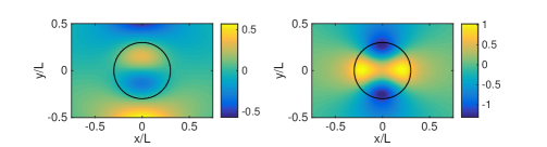
Figure 1: The imaginary (left) and real (right) parts of a normalized propagating BIC with $\omega_{*}=0.6173(2\pi c/L)$ and $\beta_{*}=0.2206(2\pi/L)$.

Fig. 1. Notice that $u_{*}$ is even in $x$. The maximum of $|u_{*}|$ is about $1.3165$.

For the nonlinear problem, we specify a plane incident plane wave with $\omega=\omega_{*}/2=0.30865\,(2\pi c/L)$ and $\beta=\beta_{*}/2=0.1103\,(2\pi/L)$, and assume the amplitude of the incident wave is $A=10^{6}$ V/m. We solve the four-wave model by the iterative scheme (63)-(66), with zero initial guesses and an error tolerance $\tau_{\rm err}=10^{-10}$. The results are shown in Fig. 2.

Figure 2: Numerical solution of the four-wave model. The imaginary and real parts of the fundamental frequency [(a) and (b)], second harmonic [(c) and (d)], third harmonic [(e) and (f)], and fourth harmonic [(g) and (h)] waves are shown in the left and right columns, respectively.

It can be seen that the second harmonic wave is indeed much stronger than the incident wave. The maximum of $|u_{2}|$ is about $1.4889\times 10^{8}$ V/m. This is very different from existing studies on SHG, where the second harmonic wave is usually very weak when $|A\gamma_{1}|\ll 1$. It can also be seen that the fourth harmonic wave is stronger than the third harmonic wave, and both of them are weaker than with the incident wave. These numerical results are obtained with $N=52$ and $M=26$.

Since $\delta=\sqrt[3]{A\gamma_{1}}=0.01$, the numerical results are consistent with the scaling suggested in section 3, i.e., $u_{1}=O(A)$, $u_{2}=O(A/\delta)$, $u_{3}=O(A\delta^{2})$ and $u_{4}=O(A\delta)$. To check the validity of the perturbation theory, we calculate the leading terms in expansions (32)-(35). We solve $u_{10}$ based on cylindrical wave expansions in $\Omega$ [30], and solve $\psi$ and $u_{30}$ in $\Omega_{c}$ by the mixed Chebyshev-Fourier pseudospectral method. The coefficient $C_{0}$ given in Eq. (52) is evaluated, and we get $C_{0}=1.0043-0.5201i$. In Fig. 3,

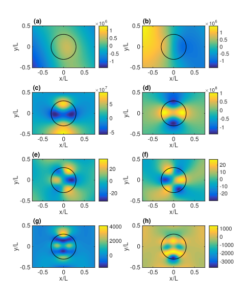
Figure 3: Leading terms in the perturbation expansions (32)-(35). The imaginary and real parts of the fundamental frequency [(a) and (b)], second harmonic [(c) and (d)], third harmonic [(e) and (f)], and fourth harmonic [(g) and (h)] waves are shown in the left and right columns, respectively.

we show the leading terms $Au_{10}$, $(AC_{0}/\delta)u_{*}$, $A\delta^{2}u_{30}$ and $A\delta u_{40}$ for $u_{1}$, $u_{2}$, $u_{3}$ and $u_{4}$, respectively. It is clear that they agree very well with the full numerical solutions shown in Fig. 2. In particular, using the values of $C_{0}$ and $\max|u_{*}|$, we get $|AC_{0}/\delta|\max|u_{*}|=1.4889\times 10^{8}$ V/m, and it agrees perfectly with value of $\max|u_{2}|$ found earlier.

For this example, we also calculate the power radiated out by waves of different frequencies based on the numerical solutions of the four-wave model. The energy conservation property $\sum_{n=1}^{4}P_{n}^{\rm out}/P_{1}^{\rm inc}=1$ is satisfied with a precision of $10^{-8}$. Although the second harmonic wave $u_{2}$ is strong, very little power is converted to it, since the dominate part of $u_{2}$ is the BIC which cannot radiate out power. Among the three harmonic waves, the fourth harmonic wave has the largest conversion efficiency, followed by the third harmonic wave and then the second harmonic wave. In the perturbation expansion (33) of $u_{2}$, the first two terms $u_{20}$ and $u_{21}$ are proportional to the BIC $u_{*}$, and only the third term $u_{22}$ can radiate out power. With $C_{0}$ determined such that the system (50)-(51) has solutions, we can calculate $u_{22}$ using the same mixed Chebyshev-Fourier pseudospectral method. As we mentioned in section 3, a unique solution for $u_{22}$ can be determined when the solvability condition for $u_{24}$ is imposed, and it can be written as $u_{22}=C_{2}u_{*}+u_{22}^{(p)}$ with $u_{22}^{(p)}$ orthogonal to $u_{*}$ on a chosen domain. In Fig. 4,

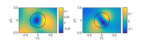
Figure 4: The imaginary (left) and real (right) parts of $A\delta^{3}u^{(p)}_{22}$, where $u^{(p)}_{22}$ is the part of $u_{22}$ orthogonal to the BIC, $u_{22}$ is the first non-BIC term in the perturbation expansion (33) of the second harmonic wave.

we show $A\delta^{3}u_{22}^{(p)}$ with the orthogonality defined on $\Omega_{c}$. The conversion efficiency for $u_{2}$ is small, since the magnitude of $A\delta^{3}u_{22}^{(p)}$ is much smaller than those of $u_{4}$ and $u_{3}$.

A periodic array of circular cylinders is a structure with reflection symmetries in both $x$ and $y$. Propagating BICs on such structures are usually regarded as unprotected by symmetry, but some of these BICs are robust under symmetry-preserving perturbations. That is, if the structure is perturbed without destroying the reflection symmetries, the BIC continues its existence with a slightly different frequency and a slightly different Bloch wavenumber [15]. For the circular array, the BIC has an existence domain in the parameter space of radius $a$ and dielectric constant $\epsilon_{1}$ [13]. The perturbation theory of section 3 is supposed to be valid for any BIC on 2D periodic structures. As a simple check, we calculate coefficient $C_{0}$ varying one of these two parameters. The results are shown in Fig. 5.

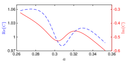
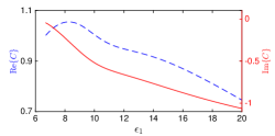
Figure 5: The real (dashed blue curve) and imaginary (solid red curve) parts of $C_{0}$ for a propagating BIC as functions of radius $a$ (left, for fixed $\epsilon_{1}=10$) and dielectric constant $\epsilon_{1}$ (right, for fixed $a=0.3L$). Real and imaginary parts follow the left and right axes.

The left and right panels show $C_{0}$ for a fixed $\epsilon_{1}=10$ and fixed $a=0.3L$, respectively. The real and imaginary parts of $C_{0}$ are shown according to the left and right vertical axes in each panel.

Since the second harmonic wave is $O(A/\delta)$, a smaller nonlinear coefficient actually produces a larger amplitude for the BIC. This may seem to be counter-intuitive, since the BIC is created by a nonlinear process, and a smaller nonlinear coefficient implies weaker nonlinear effects. However, the amplitude of the BIC only reflects the steady state where a number of sub-processes are balanced. The terms $u_{1}^{2}$ and $u_{2}^{2}$ in the right hand sides of Eqs. (16) and (18) correspond to the SHG processes from $\omega$ to $2\omega$ and from $2\omega$ to $4\omega$, respectively. Power is converted to the second harmonic wave by the first SHG process, and removed from it by the second SHG process. A smaller nonlinear coefficient reduces the ratio between the amplitudes of $u_{4}$ and $u_{2}$, but it does not reduce the ratio between $u_{2}$ and $u_{1}$, since the second harmonic wave can accumulate in the BIC. As we mentioned in section 3, the term $\bar{u}_{2}u_{4}$ in the right hand side of Eq. (16) must have the same order as $u_{1}^{2}$, therefore, a smaller nonlinear coefficient will produce a stronger second harmonic wave. If we consider a time-dependent problem by turning on the incident wave at $t=0$, a smaller nonlinear coefficient implies that longer time is needed to reach the steady state.

The excitation of a BIC of $O(A/\delta)$ by an incident wave of amplitude $A$ is only possible when $C_{0}\neq 0$. It is important to note that $C_{0}=0$ for anti-symmetric standing waves on symmetric periodic structures. Here, the reflection symmetry in the periodic direction $y$ is concerned. The dielectric function of the periodic structure is assumed to be even in $y$, while the BIC mode profile $u_{*}$ is odd in $y$, and the Bloch wavenumber $\beta_{*}=0$. The anti-symmetric standing waves are well-known symmetry-protected BICs. The linear solution $u_{10}$ is an even function of $y$, since $\beta_{*}=0$ implies a normal incident wave. The function $F=F(x,y)$ is also even in $y$, thus $C_{0}$ given in Eq. (52) is automatically zero. For such a case, it can be shown that the leading terms for second, third and fourth harmonic waves are $O(A\delta^{3})$, $O(A\delta^{6})$ and $O(A\delta^{9})$, respectively, and it is sufficient to use the two-wave model. For $a=0.3L$ and $\epsilon_{1}=10$, the periodic array of circular cylinders has an anti-symmetric standing wave with $\omega_{*}=0.4415\,(2\pi c/L)$ and $\beta_{*}=0$. We have solved the four-wave model with same incident wave amplitude $A=10^{6}$ V/m and nonlinear coefficient $\gamma_{1}=10^{-12}$ m/V, confirmed that the second harmonic wave is weak, and the higher harmonic waves are extremely weak.

6 Conclusion

The diffraction of a plane wave by a periodic structure is the subject of many theoretical, numerical and experimental studies. Nonlinear diffraction problems give rise to many interesting wave phenomena and have useful practical applications. For periodic structures with a second order nonlinearity, existing studies are concerned with the SHG process for which it is sufficient to include only the fundamental and second harmonic waves. In this paper, we also consider periodic structures with a second order nonlinearity, but assume that the corresponding linear periodic structure has a BIC and the incident wave has half the BIC frequency and a compatible wavevector. It turns out that the nonlinear diffraction problem under these assumptions is very different from the standard SHG process. The incident wave may induce a very strong second harmonic wave dominated by the BIC, and it also induces higher harmonic waves among which the fourth harmonic wave cannot be ignored. We derive an explicit formula for the leading coefficient of the BIC using a perturbation method, and propose that a coupled system of four Helmholtz equations (the four-wave model) is sufficiently accurate for analyzing the nonlinear process. Numerical solutions based on a four-wave model are presented and used to validate the perturbation results.

The BICs on a periodic structure are guided modes above the lightline that cannot be excited by incident plane waves if the structure consists of linear materials. Our study indicates that a propagating BIC with a very large amplitude can be excited by a plane incident wave if the structure has a second order nonlinearity. Since the fourth harmonic wave has the largest power conversion efficiency, it may be possible to realize the nonlinear process studied in this paper as a useful fourth harmonic generation technique.

References

- [1] J. von Neumann and E. Wigner, über merkwürdige diskrete Eigenwerte, Phys. Z, 30 (1929), pp. 465–467.
- [2] A.-S. Bonnet-Bendhia and F. Starling, Guided waves by electromagnetic gratings and nonuniqueness examples for the diffraction problem, Math. Methods Appl. Sci., 17 (1994), pp. 305–338.
- [3] D. V. Evans, M. Levitin and D. Vassiliev, Existence theorems for trapped modes, J. Fluid Mech., 261 (1994), pp. 21–31.
- [4] Y. Plotnik, O. Peleg, F. Dreisow, M. Heinrich, S. Nolte, A. Szameit, and M. Segev, Experimental observation of optical bound states in the continuum, Phys. Rev. Lett., 107 (2011), 183901.
- [5] P. Paddon and J. F. Young, Two-dimensional vector-coupled-mode theory for textured planar waveguides, Phys. Rev. B, 61 (2000), pp. 2090–2101.
- [6] S. P. Shipman and S. Venakides, Resonance and bound states in photonic crystal slabs, SIAM J. Appl. Math., 64 (2003), pp. 322–342.
- [7] R. Porter and D. Evans, Embedded Rayleigh-Bloch surface waves along periodic rectangular arrays, Wave Motion, 43 (2005), pp. 29–50.
- [8] S. Shipman and D. Volkov, Guided modes in periodic slabs: existence and nonexistence, SIAM J. Appl. Math., 67 (2007), pp. 687–713.
- [9] D. C. Marinica, A. G. Borisov, and S. V. Shabanov, Bound states in the continuum in photonics, Phys. Rev. Lett., 100 (2008), 183902.
- [10] C. W. Hsu, B. Zhen, J. Lee, S.-L. Chua, S. G. Johnson, J. D. Joannopoulos, and M. Soljačić, Observation of trapped light within the radiation continuum, Nature, 499 (2013), pp. 188–191.
- [11] E. N. Bulgakov and A. F. Sadreev, Bloch bound states in the radiation continuum in a periodic array of dielectric rods, Phys. Rev. A, 90 (2014), 053801.
- [12] Z. Hu and Y. Y. Lu, Standing waves on two-dimensional periodic dielectric waveguides, Journal of Optics, 17 (2015), 065601.
- [13] L. Yuan and Y. Y. Lu, Propagating Bloch modes above the lightline on a periodic array of cylinders, J. Phys. B: At. Mol. Opt. Phys., 50 (2017), 05LT01.
- [14] H. Friedrich and D. Wintgen, Interfering resonances and bound states in the continuum, Phys. Rev. A, 32 (1985), pp. 3231-3242.
- [15] L. Yuan and Y. Y. Lu, Bound states in the continuum on periodic structures: perturbation theory and robustness, Opt. Lett., 42 (2017), pp. 4490–4493.
- [16] Z. Hu and Y. Y. Lu, Resonances and bound states in the continuum on periodic arrays of slightly noncircular cylinders, J. Phys. B: At. Mol. Opt. Phys., 51 (2018), 035402.
- [17] C. W. Hsu, B. Zhen, A. D. Stone, J. D. Joannopoulos, and M. Soljačić, Bound states in the continuum, Nat. Rev. Mater., 1 (2016), 16048.
- [18] E. N. Bulgakov, K. N. Pichugin, and A. F. Sadreev, All-optical light storage in bound states in the continuum and release by demand, Opt. Expr., 23 (2015), pp. 22520–22531.
- [19] R. W. Boyd, Nonlinear Optics, 3rd Ed., Academic Press, 2008.
- [20] L. Yuan and Y. Y. Lu, Nonlinear standing waves on a periodic array of circular cylinders, Opt. Expr., 23 (2015), pp. 20636–20646.
- [21] L. Yuan and Y. Y. Lu, Diffraction of plane waves by a periodic array of nonlinear circular cylinders, Phys. Rev. A, 94 (2016), 013852.
- [22] L. Yuan and Y. Y. Lu, Strong resonances on periodic arrays of cylinders and optical bistability with weak incident waves, Phys. Rev. A, 95 (2017), 023834.
- [23] P. A. Franken, A. E. Hill, C. W. Peters, and G. Weinreich, Generation of optical harmonics, Phys. Rev. Lett., 7 (1961), pp. 118–119.
- [24] G. Bao and D. Dobson, Second harmonic generation in nonlinear optical films, J. Math. Phys., 35 (1994), pp. 1622–1633.
- [25] G. Bao and D. Dobson, Diffractive optics in nonlinear media with periodic structure, Euro. J. Appl. Math., 6 (1995), pp. 573–590.
- [26] G. Bao and Y. Chen, A nonlinear grating problem in diffractive optics, SIAM J. Math. Anal., 28 (1997), pp. 322–337.
- [27] G. Bao, D. C. Dobson and J. A. Cox, Mathematical studies in rigorous grating theory, J. Opt. Soc. Am. A, 12 (1995), pp. 1029–1042.
- [28] G. Bao and D. C. Dobson, On the scattering by a biperiodic structure, Proceedings of the American Mathematical Society, 128 (2000), pp. 2715–2723.
- [29] L. N. Trefethen, Spectral Methods in MATLAB, Society for Industrial and Applied Mathematics, 2000.
- [30] Y. Huang and Y. Y. Lu, Scattering from periodic arrays of cylinders by Dirichlet-to-Neumann maps, Journal of Lightwave Technology, 24 (2006), pp. 3448–3453.
- [31] P. A. Martin, Multiple Scattering: Interaction of Time-Harmonic Waves with Obstacles, Cambridge University Press, 2006.