Testing for Externalities in Network Formation Using Simulation

Bryan S. Grahamand Andrin Pelican^†

Initial Draft: June 2019, This Draft: July 2019

Abstract

We discuss a simplified version of the testing problem considered by Pelican & Graham, (2019): testing for interdependencies in preferences over links among $N$ (possibly heterogeneous) agents in a network. We describe an exact test which conditions on a sufficient statistic for the nuisance parameter characterizing any agent-level heterogeneity. Employing an algorithm due to Blitzstein & Diaconis, (2011), we show how to simulate the null distribution of the test statistic in order to estimate critical values and/or p-values. We illustrate our methods using the Nyakatoke risk-sharing network. We find that the transitivity of the Nyakatoke network far exceeds what can be explained by degree heterogeneity across households alone.

JEL Classification:

Keywords: Networks, Strategic Interaction, Testing, $\beta$ Model, Importance Sampling

De Weerdt, (2004) studies the formation of risk-sharing links among $N=119$ households located in the Tanzanian village of Nyakatoke. Let $\hat{P}\left(\vbox{\hbox{\includegraphics[scale={0.125}]{triangle.eps}}}\right)$ and $\hat{P}\left(\vbox{\hbox{\includegraphics[scale={0.125}]{twostar.eps}}}\right)$, respectively, equal the fraction of all $\tbinom{N}{3}$ triads which take the triangle and two-star configuration. De Weerdt, (2004) finds that the transitivity of the Nyakatoke risk-sharing network

$$\mathrm{\hat{TI}}=\frac{3\hat{P}\left(\vbox{\hbox{\includegraphics[scale={0.125}]{triangle.eps}}}\right)}{3\hat{P}\left(\vbox{\hbox{\includegraphics[scale={0.125}]{triangle.eps}}}\right)+\hat{P}\left(\vbox{\hbox{\includegraphics[scale={0.125}]{twostar.eps}}}\right)}=0.1884$$ (1)

is almost three times its density ($\hat{P}\left(\vbox{\hbox{\includegraphics[scale={0.125}]{edge.eps}}}\right)=0.0698$). There are several, not necessarily mutually exclusive, explanations for the clustering present in Nyakatoke. First, it may reflect the increased value of a risk-sharing relationship between two households when “supported” by a third household (Jackson et al.,, 2012). Households $i$ and $j$ may value a risk sharing link with each other more if they are both additionally linked to household $k$. Household $k$ may then serve as a monitor, arbiter and referee for households $i$ and $j$’s relationship (increasing its value). Second, clustering may simply be an artifact of degree heterogeneity, whereby high degree households link more frequently with one-another and hence form triangles ( ) incidentally. Third, clustering may also stem from homophilous sorting on kinship, ethnicity, religion and so on (McPherson et al.,, 2001).

In this chapter we outline a method of randomization inference, in the spirit of Fisher, (1935), that can be used to “test” for externalities, or interdependencies, in link formation. Externalities arise when the utility two agents generate when forming a link varies with the presence or absence of edges elsewhere in the network. Attaching greater utility to “supported” links is one such interdependency. Externalities typically imply that an efficient network will not form when link formation is negotiated bilaterally (e.g., Bloch & Jackson,, 2007). Consider household $i$, who is linked to $k$, an incidental consequence of $i$ additionally linking to $j$, is that she will then be able to “support” any link between $j$ and $k$. When evaluating whether to form a link with $j$, $i$ may not internalize this additional, non-bilateral, benefit; consequently, there may be too few risk-sharing links in Nyakatoke.

The scientific and policy implications of externalities are considerable (cf., Graham,, 2016). In the presence of interdependencies small re-wirings of a network may induce a cascade of link revisions, alternating network structure, as well as agents’ utility, substantially. In the absence of interdependencies links form bilaterally and re-wirings will not induce additional changes in network structure.

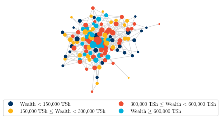
Figure 1: Nyakatoke risk-sharing network

Notes: Nodes/Households are colored according to total land and livestock wealth in Tanzanian Shillings (calculated as described by Comola & Fafchamps, (2014)). Node sizes are proportional to degree.

Source: De Weerdt, (2004) and authors’ calculations. Raw data available at https://www.uantwerpen.be/en/staff/joachim-deweerdt/ (Accessed January 2017).

Testing for externalities in network formation is not straightforward; particularly if the null model allows for rich forms of agent-level heterogeneity. Allowing for heterogeneity under the null is essential, after all, such heterogeneity provides an alternative explanation for the type of link clustering which arises in the presence of externalities.

The approach outlined here draws upon Pelican & Graham, (2019). Our goal here, however, is primarily pedagogical; to introduce some key ideas and methods likely to be of interest to empirical researchers interested in networks. Relative to what is presented here, Pelican & Graham, (2019) additionally consider (i) directed as well as undirected networks, (ii) null models which allow for both degree heterogeneity and homophily, (iii) models with and without transfers, (iv) constructing test statistics to maximize power in certain directions and (v) novel Markov Chain Monte Carlo (MCMC) methods of simulating the null distribution of the test statistic.

While the presentation in this chapter is more basic, the upshot is that the method outlined here can be implemented by combining familiar heuristics (e.g., Milo et al.,, 2002) with a little game theory and the adjacency matrix simulation algorithm of Blitzstein & Diaconis, (2011).

We begin by outlining a simple network formation game with transfers in the spirit of Bloch & Jackson, (2007). We then formally describe our test. Next we discuss how to simulate the null distribution of our test statistic using an algorithm due to Blitzstein & Diaconis, (2011); we also briefly discuss other applications of this algorithm as well as alternatives to it. We close with an illustration based upon the Nyakatoke network.

In what follows we let $\mathbf{D}$ be the adjacency matrix associated with a simple graph $G\left(\mathcal{V},\mathcal{E}\right)$ defined on $N=\left|\mathcal{V}\right|$ vertices or agents. The set $\mathcal{V}=\left\{1,\ldots,N\right\}$ includes all agents in the network and $\mathcal{E}\subseteq\mathcal{V}\times\mathcal{V}$ equals the set of undirected edges or links among them. The set of all $N\times N$ undirected adjacency matrices is denoted by $\mathbb{D}_{N}.$

A strategic network formation game with transfers

In this section we outline a simple model of strategic network formation where agents may make (bilateral) transfers to one another. Let $\nu_{i}\thinspace:\thinspace\mathbb{D}_{N}\rightarrow\mathbb{R}$ be a utility function for agent $i$, which maps adjacency matrices – equivalently networks – into utils. The marginal utility for agent $i$ associated with (possible) edge $\left(i,j\right)$ is

$$MU_{ij}\left(\mathbf{D}\right)=\left\{\begin{array}[]{cc}\nu_{i}\left(\mathbf{D}\right)-\nu_{i}\left(\mathbf{D}-ij\right)&\text{if}\thinspace D_{ij}=1\\ \nu_{i}\left(\mathbf{D}+ij\right)-\nu_{i}\left(\mathbf{D}\right)&\text{if}\thinspace D_{ij}=0\end{array}\right.$$ (2)

where $\mathbf{D}-ij$ is the adjacency matrix associated with the network obtained after deleting edge $\left(i,j\right)$ and $\mathbf{D}+ij$ the one obtained via link addition.

From Bloch & Jackson, (2006), a network is pairwise stable with transfers if the following condition holds.

Definition 1.

(Pairwise stability with Transfers) The network $G\left(\mathcal{V},\mathcal{E}\right)$ is pairwise stable with transfers if
(i) $\forall\left(i,j\right)\in\mathcal{E}\left(G\right),\thinspace MU_{ij}\left(\mathbf{D}\right)+MU_{ji}\left(\mathbf{D}\right)\geq 0$
(ii) $\forall\left(i,j\right)\notin\mathcal{E}\left(G\right),\thinspace MU_{ij}\left(\mathbf{D}\right)+MU_{ji}\left(\mathbf{D}\right)<0$

Definition 1 states that the marginal utility of all links actually present in a pairwise stable network is (weakly) positive, while that associated with links not present is negative. The definition presumes utility is transferable, since it only requires that the sum of utility to $i$ and $j$ associated with edge $\left(i,j\right)$ is positive. When the sum of the two marginal utilities is positive, there exists a within-dyad transfer such that both agents benefit. Note also that the definition is pairwise: the benefit of a link is evaluated conditional on the remaining network structure. It is possible, for example, that a coalition of players could increase their utility by jointly forming a set of links and making transfers to one another. Imposing more sophisticated play of this type would result in a refinement relative to the set of network configurations which satisfy Definition 1 (cf., Jackson,, 2008).

In this chapter we will specialize to utility functions of the form

$$\nu_{i}\left(\mathbf{d},\mathbf{U};\gamma_{0},\delta_{0}\right)=\sum_{j}d_{ij}\left[A_{i}+B_{j}+\gamma_{0}s_{ij}\left(\mathbf{d}\right)-U_{ij}\right]$$ (3)

with $\mathbf{U}=\left[U_{ij}\right]$. Here $A_{i}$ and $B_{j}$ capture agent-level degree heterogeneity (cf., Graham,, 2017). If $A_{i}$ is high, then the baseline utility associated with any link is high for agent $i$ ($i$ is an “extrovert”). If $B_{j}$ is high, then $j$ is a particularly attractive partner for all other agents ($j$ is “popular”). We leave the joint distribution of $\mathbf{A}=\left[A_{i}\right]$ and $\mathbf{B}=\left[B_{i}\right]$ unrestricted in what follows.

The $s_{ij}\left(\mathbf{d}\right)$ term is associated with externalities in link formation. We require that $s_{ij}\left(\mathbf{d}\right)=s_{ij}\left(\mathbf{d}-ij\right)=s_{ij}\left(\mathbf{d}+ij\right)$; additional restrictions might be needed to ensure the existence of a network that is pairwise stable with transfers and/or a test statistic with a non-degenerate null distribution.

Instead of formulating additional high-level conditions on $s_{ij}\left(\mathbf{d}\right)$, in what follows we emphasize, and develop results for, two specific examples. In the first $s_{ij}\left(\mathbf{d}\right)$ equals

$$s_{ij}\left(\mathbf{d}\right)=\sum_{k}d_{jk},$$ (4)

which implies that agents receive more utility from links with popular (or high degree) agents.

The second example specifies $s_{ij}\left(\mathbf{d}\right)$ as

$$s_{ij}\left(\mathbf{d}\right)=\sum_{k}d_{ik}d_{jk},$$ (5)

which implies that dyads receive more utility from linking when they share other links in common. This is a transitivity effect.

When the utility function is of the form given in (3) the marginal utility agent $i$ gets from a link with $j$ is

$$MU_{ij}\left(\mathbf{d},\mathbf{U};\gamma_{0},\delta_{0}\right)=A_{i}+B_{j}+\gamma_{0}s_{ij}\left(\mathbf{d}\right)-U_{ij}.$$

Pairwise stability then implies that, conditional on the realizations of $\mathbf{A}$, $\mathbf{B}$, $\mathbf{U}$ and the value of externality parameter $\gamma_{0}$, the observed network must satisfy, for $i=1,\ldots,N-1$ and $j=i+1,\ldots,N$

$$D_{ij}=\mathbf{1}\left(\tilde{A}_{i}+\tilde{A}_{j}+\gamma_{0}\tilde{s}_{ij}\left(\mathbf{d}\right)\geq\tilde{U}_{ij}\right)$$ (6)

with $\tilde{A}_{i}=A_{i}+B_{i}$, $\tilde{s}_{ij}\left(\mathbf{d}\right)=s_{ij}\left(\mathbf{d}\right)+s_{ji}\left(\mathbf{d}\right)$ and $\tilde{U}_{ij}=U_{ij}+U_{ji}$.

Equation (6) defines a system of $\tbinom{N}{2}=\frac{1}{2}N\left(N-1\right)$ nonlinear simultaneous equations. Any solution to this system – and there will typically be multiple ones – constitutes a pairwise stable (with transfers) network. To make this observation a bit more explicit, similar to Miyauchi, (2016), consider the mapping $\varphi\left(\mathbf{D}\right)\thinspace:\thinspace\mathbb{D}_{N}\rightarrow\mathbb{I}_{\tbinom{N}{2}}$:

$$\varphi\left(\mathbf{d}\right)\equiv\left[\begin{array}[]{c}\mathbf{1}\left(\tilde{A}_{1}+\tilde{A}_{2}+\gamma_{0}\tilde{s}_{12}\left(\mathbf{d}\right)\geq U_{12}\right)\\ \mathbf{1}\left(\tilde{A}_{1}+\tilde{A}_{3}+\gamma_{0}\tilde{s}_{13}\left(\mathbf{d}\right)\geq U_{13}\right)\\ \vdots\\ \mathbf{1}\left(\tilde{A}_{N-1}+\tilde{A}_{N}+\gamma_{0}\tilde{s}_{N-1N}\left(\mathbf{d}\right)\geq U_{N-1N}\right)\end{array}\right].$$ (7)

Under the maintained assumption that the observed network satisfies Definition 1, the observed adjacency matrix corresponds to the fixed point

$$\mathbf{D}=\text{vech}^{-1}\left[\varphi\left(\mathbf{D}\right)\right].$$

Here $\mathrm{vech}(\cdot)$ vectorizes the $\tbinom{N}{2}$ elements in the lower triangle of an $N\times N$ matrix and we define its inverse operator as creating a symmetric matrix with a zero diagonal. In addition to the observed network there may be other $\mathbf{d}\in\mathbb{D}_{N}$ such that $\mathbf{d}=\text{vech}^{-1}\left[\varphi\left(\mathbf{d}\right)\right]$. The fixed point representation is useful for showing equilibrium existence as well as for characterization (e.g., using Tarski’s (1955) fixed point theorem).

For the two types of network formation externalities we consider, specified in equations (4) and (5) above, the $\varphi\left(\mathbf{d}\right)$ mapping is weakly increasing in $\mathbf{d}$ for $\gamma_{0}\geq 0$. This allows for the application of Tarski’s (1955) theorem; ensuring existence of at least one pairwise stable equilibrium.

Test formulation

Our goal is to assess the null hypothesis that $\gamma_{0}=0$ relative to the alternative that $\gamma_{0}>0$. The extension of what follows to two-sided tests is straightforward. A feature our testing problem is the presence of a high-dimensional nuisance parameter in the form of the $N$ degree heterogeneity terms, $\mathbf{\tilde{A}}=\left[\tilde{A}_{i}\right]$. Since the value of these terms may range freely over the null, our null hypothesis is a composite one.

The composite nature of the null hypothesis raises concerns about size control. Ideally our test will have good size properties regardless of the particular value of $\mathbf{\tilde{A}}$. Assume, for example, that the distribution of the $\left\{\tilde{A}_{i}\right\}_{i=1}^{N}$ is right-skewed. In this case we will likely observe high levels of clustering among high $\tilde{A}_{i}$ agents. Measured transitivity in the network might be substantial even in the absence of any structural preference for transitive relationships. We want to avoid excessive rejection of our null hypothesis in such settings; we do so by varying the critical value used for rejection with the magnitude of a sufficient statistics for the $\left\{\tilde{A}_{i}\right\}_{i=1}^{N}$.

A simple example helps to fix ideas. Under the null we have, for $i=1,\ldots,N-1$ and $j=i+1,\ldots,N$,

$$\Pr\left(D_{ij}=1\right)=\frac{\exp\left(\tilde{A}_{i}+\tilde{A}_{j}\right)}{1+\exp\left(\tilde{A}_{i}+\tilde{A}_{j}\right)},$$ (8)

which corresponds to the $\beta$-model of network formation (e.g., Chatterjee et al.,, 2011). Assume that $\tilde{A}_{i}\in\left\{-\infty,\frac{1}{2}\ln\left(\frac{\rho}{1-\rho}\right)\right\}$ with $\tilde{A}_{i}=-\infty$ with probability $1-\pi$. In this simple model two “high” $\tilde{A}_{i}$ agents link with probability $\rho$, while low-to-low and low-to-high links never form. Some simple calculations give an overall density for this network of $\pi^{2}\rho$, and a (population) transitivity index of $\rho$. For $\pi$ small and or $\rho$ large, transitivity in this network may exceed density substantially even though there is no structural taste for transitive links among agents. Here the transitivity is entirely generated by high degree agents linking with one another with greater frequency and, only incidentally, forming triangles in the process. A simple comparison of density and transitivity in this case is uninformative.

Motivated in part by this inferential challenge, as well as to exploit classic results on testing in exponential families (e.g., Lehmann & Romano,, 2005, Chapter 4), it will be convenient in what follows to assume that $\tilde{U}_{ij}\sim\text{Logistic}\left(0,1\right)$. Next let $\mathbb{A}$ denoting a subset of the $N$ dimensional Euclidean space in which $\tilde{\mathbf{A}}$ is, a priori, known to lie, and

$$\Theta_{0}=\left\{\left(\gamma,\tilde{\mathbf{A}}^{\prime}\right)\thinspace:\thinspace\gamma=0,\tilde{\mathbf{A}}\in\mathbb{A}\right\}.$$

Our null hypothesis is

$$H_{0}\thinspace:\thinspace\theta\in\Theta_{0}$$ (9)

since $\tilde{\mathbf{A}}$ may range freely over $\mathbb{A}\subset\mathbb{R}^{N}$ under the null of no externalities in link formation ($\gamma_{0}=0$). With a little manipulation we can show that, under (9), the probability of the event $\mathbf{D}=\mathbf{d}$ takes the exponential family form

$$P_{0}\left(\mathbf{d};\tilde{\mathbf{A}}\right)=c\left(\tilde{\mathbf{A}}\right)\exp\left(\mathbf{d}_{+}^{\prime}\tilde{\mathbf{A}}\right)$$

with $\mathbf{d}_{+}=\left(d_{1+},\ldots,d_{N+}\right)$ equal to the degree sequence of the network.

Let $\mathbb{D}_{N,\mathbf{\mathbf{d}_{+}}}$ denote the set of all undirected $N\times N$ adjacency matrices with degree counts also equal to $\mathbf{d}_{+}$ and $\left|\mathbb{D}_{N,\mathbf{\mathbf{d}_{+}}}\right|$ denote the size, or cardinality, of this set. Under $H_{0}$ the conditional likelihood of $\mathbf{D}=\mathbf{d}$ given $\mathbf{D_{+}=d_{+}}$ is

$$P_{0}\left(\left.\mathbf{d}\right|\mathbf{D_{+}=d_{+}}\right)=\frac{1}{\left|\mathbb{D}_{N,\mathbf{\mathbf{d}_{+}}}\right|}.$$

Under the null of no externalities all networks with identical degree sequences are equally probable. This insight will form the basis of our test.

Let $T\left(\mathbf{d}\right)$ be some statistic of the adjacency matrix $\mathbf{D}=\mathbf{d}$, say its transitivity index. We work with a (test) critical function of the form

$$\phi\left(\mathbf{d}\right)=\left\{\begin{array}[]{cc}1&T\left(\mathbf{d}\right)>c_{\alpha}\left(\mathbf{d}_{+}\right)\\ g_{\alpha}\left(\mathbf{d}_{+}\right)&T\left(\mathbf{d}\right)=c_{\alpha}\left(\mathbf{d}_{+}\right)\\ 0&T\left(\mathbf{d}\right)<c_{\alpha}\left(\mathbf{d}_{+}\right)\end{array}\right..$$

We will reject the null if our statistic exceeds some critical value, $c_{\alpha}\left(\mathbf{d}_{+}\right)$ and accept it – or fail to reject it – if our statistic falls below this critical value. If our statistic exactly equals the critical value, then we reject with probability $g_{\alpha}\left(\mathbf{d}_{+}\right)$. The critical value $c_{\alpha}\left(\mathbf{d}_{+}\right)$, as well as the probability $g_{\alpha}\left(\mathbf{d}_{+}\right)$, are chosen to set the rejection probability of our test under the null equal to $\alpha$ (i.e., to control size). In order to find the appropriate values of $c_{\alpha}\left(\mathbf{d}_{+}\right)$ and $g_{\alpha}\left(\mathbf{d}_{+}\right)$ we need to know the distribution of $T\left(\mathbf{D}\right)$ under the null.

Conceptually this distribution is straightforward to characterize; particularly if we proceed conditional on the degree sequence observed in the network in hand. Under the null all possible adjacency matrices with degree sequence $\mathbf{d}_{+}$ are equally probable. The null distribution of $T\left(\mathbf{D}\right)$ therefore equals its distribution across all these matrices. By enumerating all the elements of $\mathbb{D}_{N,\mathbf{\mathbf{d}_{+}}}$ and calculating $T\left(\mathbf{d}\right)$ for each one, we could directly – and exactly – compute this distribution. In practice this is not (generally) computationally feasible. Even for networks that include as few as 10 agents, the set $\mathbb{D}_{N,\mathbf{\mathbf{d}_{+}}}$ may have millions of elements (see, for example, Table 1 of Blitzstein & Diaconis, (2011)). Below we show how to approximate the null distribution of $T\left(\mathbf{D}\right)$ by simulation, leading to a practical method of finding critical values for testing.

If we could efficiently enumerate the elements of $\mathbb{D}_{N,\mathbf{\mathbf{d}_{+}}}$ we would find $c_{\alpha}\left(\mathbf{d}_{+}\right)$ by solving

$$\Pr\left(\left.T\left(\mathbf{D}\right)\geq c_{\alpha}\left(\mathbf{d}_{+}\right)\right|\mathbf{D}\in\mathbb{D}_{\mathbf{N,\mathbf{d}_{+}}}\right)=\frac{\sum_{\mathbf{D}\in\mathbb{D}_{\mathbf{N,\mathbf{d}_{+}}}}\mathbf{1}\left(T\left(\mathbf{D}\right)\geq c_{\alpha}\left(\mathbf{d}_{+}\right)\right)}{\left|\mathbb{D}_{N,\mathbf{\mathbf{d}_{+}}}\right|}=\alpha.$$ (10)

If there is no $c_{\alpha}\left(\mathbf{d}_{+}\right)$ for which (10) exactly holds, then we would instead find the smallest $c_{\alpha}\left(\mathbf{d}_{+}\right)$ such that $\Pr\left(\left.T\left(\mathbf{D}\right)>c_{\alpha}\left(\mathbf{d}_{+}\right)\right|\mathbf{D}\in\mathbb{D}_{\mathbf{N,\mathbf{d}_{+}}}\right)\geq\alpha$ and choose $g_{\alpha}\left(\mathbf{d}_{+}\right)$ to ensure correct size.

Alternatively we might instead calculate the p-value:

$$\Pr\left(\left.T\left(\mathbf{D}\right)\geq T\left(\mathbf{d}_{+}\right)\right|\mathbf{D}\in\mathbb{D}_{\mathbf{N,\mathbf{d}_{+}}}\right)=\frac{\sum_{\mathbf{D}\in\mathbb{D}_{\mathbf{N,\mathbf{d}_{+}}}}\mathbf{1}\left(T\left(\mathbf{D}\right)\geq T\left(\mathbf{d}_{+}\right)\right)}{\left|\mathbb{D}_{N,\mathbf{\mathbf{d}_{+}}}\right|}.$$ (11)

If this probability is very low, say less than 5 percent of all networks in $\mathbb{D}_{\mathbf{N,\mathbf{d}_{+}}}$ have a transitivity index larger than the one observed in the network in hand, then we might conclude that our network is “unusual” and, more precisely, that it is not a uniform random draw from $\mathbb{D}_{\mathbf{N,\mathbf{d}_{+}}}$ (our null hypothesis).

Below we show how to approximate the probabilities to the left of the equalities in (10) and (11) by simulation.

Similarity of the test

In our setting, a test $\phi\left(\mathbf{D}\right)$, will have size $\alpha$ if its null rejection probability (NRP) is less than or equal to $\alpha$ for all values of the nuisance parameter:

$$\underset{\theta\in\Theta_{0}}{\sup}\thinspace\mathbb{E}_{\theta}\left[\phi\left(\mathbf{D}\right)\right]=\underset{\mathbf{\tilde{A}}\in\mathbb{A}}{\sup}\thinspace\mathbb{E}_{\theta}\left[\phi\left(\mathbf{D}\right)\right]=\alpha.$$

Since $\tilde{\mathbf{A}}$ is high dimensional, size control is non-trivial. This motivates, as we have done, proceeding conditionally on the degree sequence.

Let $\mathbb{D}_{+}$ be the set of all graphical degree sequences (see below for a discussion of “graphic” integer sequences). For each $\mathbf{d_{+}}\in\mathbb{D_{+}}$ our approach is equivalent to forming a test with the property that, for all $\theta\in\Theta_{0}$,

$$\mathbb{E}_{\theta}\left[\left.\phi\left(\mathbf{D}\right)\right|\mathbf{D_{+}}=\mathbf{d}_{+}\right]=\alpha.$$ (12)

Such an approach ensures similarity of our test since, by iterated expectations

$$\mathbb{E}_{\theta}\left[\phi\left(\mathbf{D}\right)\right]=\mathbb{E}_{\theta}\left[\mathbb{E}_{\theta}\left[\left.\phi\left(\mathbf{D}\right)\right|\mathbf{\mathbf{D_{+}}}\right]\right]=\alpha$$

for any $\theta\in\Theta_{0}$ (cf., Ferguson,, 1967). By proceeding conditionally we ensure the NRP is unaffected by the value of the degree heterogeneity distribution $\left\{\tilde{A}_{i}\right\}_{i=1}^{N}$. Similar tests have proved to be attractive in other settings with composite null hypotheses (cf., Moreira,, 2009).

Choosing the test statistic

Ideally the critical function is chosen to maximize the probability of correctly rejecting the null under particular alternatives of interest. It turns out that, because our network formation model is incomplete under the alternative (as we have been silent about equilibrium selection), constructing tests with good power is non-trivial. In Pelican & Graham, (2019) we show how to choose the critical function, or equivalently the statistic $T\left(\mathbf{d}\right)$, to maximize power against particular (local) alternatives. The argument is involved, so here we confine ourselves to a more informal development.

An common approach to choosing a test statistic, familiar from other applications of randomization testing (e.g., Cox,, 2006, Chapter 3), is to proceed heuristically. This suggests, for example, choosing $T\left(\mathbf{D}\right)$ to be the transitivity index, or the support measure of Jackson et al., (2012), if the researcher is interested in “testing” for whether agents prefer transitive relationships.

A variation on this approach, inspired by the more formal development in Pelican & Graham, (2019), is to set $T\left(\mathbf{D}\right)$ equal to

$$T\left(\mathbf{D}\right)=\sum_{i<j}\left(D_{ij}-\hat{p}_{ij}\right)\tilde{s}_{ij}\left(\mathbf{d}\right)$$ (13)

with $\hat{p}_{ij}=\frac{\exp\left(\hat{\tilde{A}}_{i}+\hat{\tilde{A}}_{j}\right)}{1+\exp\left(\hat{\tilde{A}}_{i}+\hat{\tilde{A}}_{j}\right)}$ and $\hat{\tilde{\mathbf{A}}}=\left[\hat{\tilde{A}}_{i}\right]$ the maximum likelihood estimate (MLE) of $\tilde{\mathbf{A}}$. The intuition behind (13) is as follows: if it is positive, this implies that high values of the externality term, $\tilde{s}_{ij}\left(\mathbf{d}\right)$, are associated with links that have low estimated probability under the null (such that $D_{ij}-\hat{p}_{ij}$ is large). The conjunction of “surprising” links with large values of $\tilde{s}_{ij}\left(\mathbf{d}\right)$ is taken as evidence that $\gamma_{0}>0$.

Consider the transitivity example with $\tilde{s}_{ij}\left(\mathbf{d}\right)=2\sum_{k}d_{ik}d_{jk}$; statistic (13), with some manipulation, can be shown to equal

$$T\left(\mathbf{D}\right) =6\left[\sum_{i<j<k}D_{ij}D_{ik}D_{jk}-\sum_{i<j<k}\frac{1}{3}\left(\hat{p}_{ij}D_{ik}D_{jk}+D_{ij}\hat{p}_{ik}D_{jk}+D_{ij}D_{ik}\hat{p}_{jk}\right)\right].$$ (14)

Statistic (14) is a measure of the difference between the actual number of triangles in the network and (a particular) expected triangle count computed under the null. To see this assume, as would be approximately true if the graph were an Erdös-Rényi one, that $\hat{p}_{ij}=\text{$\hat{P}\left(\vbox{\hbox{\includegraphics[scale={0.125}]{edge.eps}}}\right)$}$ for all $i<j$. Recalling that $\hat{P}\left(\vbox{\hbox{\includegraphics[scale={0.125}]{triangle.eps}}}\right)$ and $\hat{P}\left(\vbox{\hbox{\includegraphics[scale={0.125}]{twostar.eps}}}\right)$ respectively equal the fraction of all $\tbinom{N}{3}$ triads which are triangles and two-stars, we would have

$$T\left(\mathbf{D}\right)=2\tbinom{N}{3}\left[3\hat{P}\left(\vbox{\hbox{\includegraphics[scale={0.125}]{triangle.eps}}}\right)-\left(3\hat{P}\left(\vbox{\hbox{\includegraphics[scale={0.125}]{triangle.eps}}}\right)+\hat{P}\left(\vbox{\hbox{\includegraphics[scale={0.125}]{twostar.eps}}}\right)\right)\hat{P}\left(\vbox{\hbox{\includegraphics[scale={0.125}]{edge.eps}}}\right)\right].$$

The term in $\left[\right]$ equals the difference between the numerator of the transitivity index and its denominator times density. For an Erdös-Rényi graph this difference should be approximately zero. In the presence of degree heterogeneity, the second term to the right of the equality in (14) is a null-model-assisted count of the expected number of triangles in $G$. A rejection therefore occurs when many “surprising” triangles are present.

Before describing how to simulate the null distribution of $T\left(\mathbf{D}\right)$ we briefly recap. We start by specifying a sharp null hypothesis. Consider the network in hand with adjacency matrix $\mathbf{D}=\mathbf{d}$ and corresponding degree sequence $\mathbf{D}_{+}=\mathbf{d}_{+}$. Our null hypothesis is that the observed network coincides with a uniform random draw from $\mathbb{D}_{N,\mathbf{\mathbf{d}_{+}}}$ (i.e., the set of all networks with identical degree sequences). This null is a consequence of the form on the transferable utility network formation game outlined earlier. The testing procedure is to compare a particular statistic of $\mathbf{D}=\mathbf{d}$, say $T\left(\mathbf{d}\right)$, with its distribution across $\mathbb{D}_{N,\mathbf{\mathbf{d}_{+}}}$. If the observed value of $T\left(\mathbf{d}\right)$ is unusually large we take this as evidence against our null.

Although we have motivated our test as one for strategic interactions or externalities, in actuality we are really assessing the adequacy of a particular null model of network formation – namely the $\beta$-model. Our test may detect many types of violations of this model, albeit with varying degrees of power. Consequently we need to be careful about how we interpret a rejection in practice. At the same time, by choosing the test statistic $T\left(\mathbf{D}\right)$ with some care, we hope to generate good power to detect the violation of interest – that $\gamma_{0}>0$ – and hence conclude that externalities in link formation are likely present when we reject.

Simulating undirected networks with fixed degree

This section describes an algorithm, introduced by Blitzstein & Diaconis, (2011), for sampling uniformly from the set $\mathbb{D}_{N,\mathbf{\mathbf{d}_{+}}}$. Our notation and exposition tracks that of Blitzstein & Diaconis, (2011), albeit with less details. As noted previously, direct enumeration of all the elements of $\mathbb{D}_{N,\mathbf{\mathbf{d}_{+}}}$ is generally not feasible. We therefore require a method of sampling from $\mathbb{D}_{N,\mathbf{\mathbf{d}_{+}}}$ uniformly and also, at least implicitly, estimating its size. The goal is to replace, for example, the exact p-value (11) with the simulation estimate

$$\hat{\Pr}\left(\left.T\left(\mathbf{D}\right)\geq T\left(\mathbf{d}\right)\right|\mathbf{D}\in\mathbb{D}_{\mathbf{N,\mathbf{d}_{+}}}\right)=\frac{1}{B}\sum_{b=1}^{B}\mathbf{1}\left(T\left(\mathbf{D}_{b}\right)\geq T\left(\mathbf{d}\right)\right),$$ (15)

where $\mathbf{D}_{b}$ is a uniform random draw from $\mathbb{D}_{N,\mathbf{\mathbf{d}_{+}}}$ and $B$ denotes the number of independent simulation draws selected by the researcher.

Two complications arise. First, it is not straightforward to construct a random draw from $\mathbb{D}_{N,\mathbf{\mathbf{d}_{+}}}$. Second, we must draw uniformly from this set. Fortunately the first challenge is solvable using ideas from the discrete math literature. Researchers in graph theory and discrete math have studied the construction of graphs with fixed degrees and, in particular, provided conditions for checking whether a particular degree sequence is graphical (e.g., Sierksma & Hoogeveen,, 1991). We say that $\mathbf{d}_{+}$ is graphical if there is feasible undirected network with degree sequence $\mathbf{d}_{+}$. Not all integer sequences are graphical. The reader can verify, for example, that there is no feasible undirected network of three agents with degree sequence $\mathbf{d}_{+}=\left(3,2,1\right)$.

As for the second complication, although we can not easily/directly construct a uniform random draw from $\mathbb{D}_{N,\mathbf{\mathbf{d}_{+}}}$, we can use importance sampling (e.g., Owen,, 2013) to estimate expectations with respect to this distribution.

The basic idea and implementation is due to Blitzstein & Diaconis, (2011). A similar, and evidently independently derived, algorithm is presented in Del Genio et al., (2010). While computationally faster approaches are now available, we nevertheless present the method introduced by Blitzstein & Diaconis, (2011) for it pedagogical value and easy implementation. Their approach is adequate for small to medium sized problems. Readers interested in applying the methods outlined below to large sparse graphs might consult Rao et al., (1996), McDonald et al., (2007) or Zhang & Chen, (2013). Pelican & Graham, (2019) introduce a more complicated MCMC simulation algorithm that holds additional graph statistics constant (besides the degree sequence). They also provide references to the fairly extensive literature on adjacency matrix simulation.

While our presentation of the Blitzstein & Diaconis, (2011) algorithm is motivated by a particular formal testing problem, our view is that it is also useful for more informally finding “unusual” or “interesting” features of a given network. Are links more transitive than one would expect in networks with similar degree sequences? Is average path length exceptionally short? For this reason, the material presented below may also enter a researcher’s workflow during the data summarization or exploratory analysis stage.

The algorithm

A sequential network construction algorithm begins with a matrix of zeros and sequentially adds links to it until its rows and columns sum to the desired degree sequence. Unfortunately, unless the links are added appropriately, it is easy to get “stuck” (in the sense that at a certain point in the process it becomes impossible to reach a graph with the desired degree and the researcher must restart the process). The paper by Snijders, (1991) provides examples and discussion of this phenomena.

As an example consider the graphical degree sequence $\mathbf{d}_{+}=(2,2,1,1).$ If we begin with an empty graph and add an edge between agents 3 and 4, we will go from the degree sequence $(2,2,1,1)$ to a residual one of $(2,2,0,0)$. Unfortunately $(2,2,0,0)$ is not graphical. Adding more edges requires introducing self-loops or a double-edge, neither of which is allowed.

Intuitively we can avoid this phenomenon by first connecting high degree agents. Havel, (1955) and Hakimi, (1962) showed that this idea works for any degree sequence

Theorem 1.

(Havel-Hakimi) Let $d_{i+}>0$, if $\mathbf{d}_{+}$ does not have at least $d_{i+}$ positive entries other than $i$ it is not graphical. Assume this condition holds. Let $\mathbf{\tilde{d}}_{+}$ be a degree sequence of length $N-1$ obtained by
  [i] deleting the $i^{th}$ entry of $\mathbf{d}_{+}$ and
  [ii] subtracting 1 from each of the $d_{i+}$ highest elements in $\mathbf{d}_{+}$ (aside from the $i^{th}$ one).
$\mathbf{d}_{+}$ is graphical if and only if $\mathbf{\tilde{d}}_{+}$ is graphical. If $\mathbf{d}_{+}$ is graphical, then it has a realization where agent $i$ is connected to any of the $d_{i+}$ highest degree agents (other than $i$).

Theorem 1 gives a verifiable condition for whether a degree sequence is graphical. Blitzstein & Diaconis, (2011) extended this condition so that we can check whether a degree sequence is graphical if one node is already connected to some other nodes. This modified condition serves as a tool in their importance sampling algorithm.

Theorem 1 is suggestive of a sequential approach to building an undirected network with degree sequence $\mathbf{d}_{+}$. The procedure begins with a target degree sequence $\mathbf{d}_{+}$. It starts by choosing a link partner for the lowest degree agent (with at least one link). It chooses a partner for this agent from among those with higher degree. A one is then subtracted from the lowest degree agent and her chosen partner’s degrees. This procedure continues until the residual degree sequence (the sequence of links that remain to be chosen for each agent) is a vector of zeros.

To formally describe such an approach we require some additional notation. Let $\left(\oplus_{i_{1},\ldots,i_{k}}\mathbf{d}_{+}\right)$ be the vector obtained by adding a one to the $i_{1},\ldots,i_{k}$ elements of $\mathbf{d}_{+}$:

$$\left(\oplus_{i_{1},\ldots,i_{k}}\mathbf{d}_{+}\right)_{j}=\left\{\begin{array}[]{ll}d_{j+}+1&\mbox{for}\,j\in\left\{i_{1},\ldots,i_{k}\right\}\\ d_{j+}&\mbox{otherwise}\end{array}\right.$$

Let $\left(\ominus_{i_{1},\ldots,i_{k}}\mathbf{d}_{+}\right)$ be the vector obtained by subtracting one from the $i_{1},\ldots,i_{k}$ elements of $\mathbf{d}_{+}$:

$$\left(\ominus_{i_{1},\ldots,i_{k}}\mathbf{d}_{+}\right)_{j}=\left\{\begin{array}[]{ll}d_{j+}-1&\mbox{for}\,j\in\left\{i_{1},\ldots,i_{k}\right\}\\ d_{j+}&\mbox{otherwise}\end{array}\right.$$

Algorithm 1.

(Blitzstein and Diaconis)A sequential algorithm for constructing a random graph with degree sequence $\mathbf{d}_{+}=\left(d_{1+},\ldots,d_{N+}\right)^{\prime}$ is

1. Let $\mathbf{D}$ be an empty adjacency matrix.

2. If $\mathbf{d}_{+}=\mathbf{0}$ terminate with output $\mathbf{D}$

3. Choose the agent $i$ with minimal positive degree $d_{i+}$.

4. Construct a list of candidate partners $\mathcal{J}=\left\{j\neq i\,:\,D_{ij}=D_{ji}=0\,\mbox{and\,}\ominus_{i,j}\mathbf{d}_{+}\,\mbox{graphical}\right\}$.

5. Pick a partner $j\in\mathcal{J}$ with probability proportional to its degree in $\mathbf{d}_{+}$.

6. Set $D_{ij}=D_{ji}=1$ and update $\mathbf{d}_{+}$ to $\ominus_{i,j}\mathbf{d}_{+}$.

7. Repeat steps 4 to 6 until the degree of agent $i$ is zero.

8. Return to step 2.

The input for Algorithm 1 is the target degree sequence $\mathbf{d}_{+}$ and the output is an undirected adjacency matrix $\mathbf{D}\in\mathbb{D}_{\mathbf{N,\mathbf{d}_{+}}}$ (i.e., with $\mathbf{D}^{\prime}\iota=\mathbf{d}_{+}$).

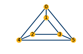
Figure 2: Cubic graph with six agents

Notes: Prism graph (a 3-regular graph) on six vertices.

Sources: Authors’ calculations.

Consider the 3-regular (i.e., cubic graph) depicted in Figure 2. Each agent in this graph has exactly three links such that its degree sequence equals $\left(3,3,3,3,3,3\right)$. In turns out that there are two non-isomorphic cubic graphs on six vertices: the prism graph, shown in the figure, and the utility graph (or complete bipartite graph on two sets of three vertices). We can use Algorithm 1 to generate a random draw from the set of all graphs with a degree sequence of $\mathbf{d}_{+}=\left(3,3,3,3,3,3\right)$.

As an example of a series of residual degree sequences (updated in Step 6 of the algorithm) associated with a random draw from $\mathbb{D}_{\mathbf{N,\mathbf{d}_{+}}}$, for $N=6$ and $\mathbf{d}_{+}=\left(3,3,3,3,3,3\right)$, consider:

$$\left(\mathbf{3},3,3,3,3,3\right) \rightarrow\left(\mathbf{2},2,3,3,3,3\right)\rightarrow\left(\mathbf{1},2,3,3,2,3\right)\rightarrow\left(0,\mathbf{2},2,3,2,3\right)$$

$$\rightarrow\left(0,\boldsymbol{1},2,3,2,2\right)\rightarrow\left(0,0,\mathbf{2},2,2,2\right)\rightarrow\left(0,0,\mathbf{1},2,1,2\right)$$

$$\rightarrow\left(0,0,0,\mathbf{2},1,1\right)\rightarrow\left(0,0,0,\mathbf{1},0,1\right)\rightarrow\left(0,0,0,0,0,0\right).$$

Labelling agents $i=0,1,\ldots,5$ from left-to-right we can see that the first link is added between agents 0 and 1 (the “active” node’s residual degree is bold-faced above). This is illustrated in Figure 3, which begins with the labelled empty graph in the upper-left-hand corner and then sequentially adds links as we move from left-to-right and top-to-bottom. Next a link is added between agents 0 and 4, and then between agents 0 and 2. Observe that the algorithm selected agent 0 as the lowest degree agent in the initial step and continues to connect this vertex with higher degree ones until all needed edges incident to it are present.

In the 8th iteration of the algorithm an edge is added between agents 3 and 4. If, instead, an edge was added between agents 4 and 5 at this point, the residual sequence degree sequence would have been updated to $\left(0,0,0,2,0,0\right)$, which is not graphic. Step 4 of the algorithm prevents the addition of edges which, if added, lead to non-graphic degree sequences. It is in this way that the algorithm avoids getting “stuck”. Getting stuck was a problem with earlier approaches to binary matrix simulation, such as the method of Snijders, (1991).

Importance sampling

Algorithm 1 produces a random draw from $\mathbb{D}_{N,\mathbf{\mathbf{d}_{+}}}$, however, it does not draw from this set uniformly. A key insight of Blitzstein & Diaconis, (2011) is that one can construct importance sampling weights to correct for non-uniformity of the draws from $\mathbb{D}_{N,\mathbf{\mathbf{d}_{+}}}$.

Let $\mathcal{\mathbb{Y}}_{N,\mathbf{d}_{+}}$ denote the set of all possible sequences of links outputted by Algorithm 1 given input $\mathbf{d}_{+}$. Let $\mathcal{D}\left(Y\right)$ be the adjacency matrix induced by link sequence $Y$. Let $Y$ and $Y^{\prime}$ be two different sequences produced by the algorithm. These sequences are equivalent if their “end point” adjacency matrices coincide (i.e., if $\mathcal{D}\left(Y\right)=\mathcal{D}\left(Y^{\prime}\right)$). We can partition $\mathcal{\mathbb{Y}}_{N,\mathbf{d}_{+}}$ into a set of equivalence classes, the number of such classes coincides with the number of feasible networks with degree distribution $\mathbf{d}_{+}$ (i.e., with the cardinality of $\mathbb{D}_{N,\mathbf{\mathbf{d}_{+}}}$).

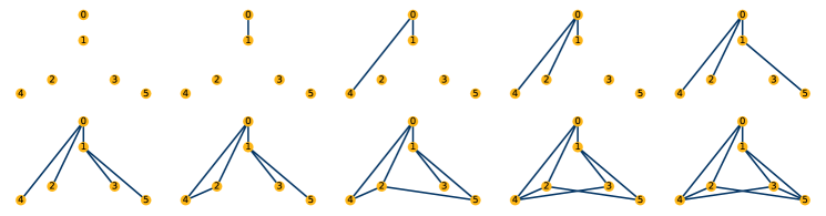
Figure 3: Simulation example

Notes: Illustration of the construction of a random draw from $\mathbb{D}_{N,\mathbf{d}_{+}}$, for $N=6$ and $\mathbf{d}_{+}=\left(3,3,3,3,3,3\right)$, as generated according to Algorithm 1.

Sources: Authors’ calculations.

Let $c\left(Y\right)$ denote the number of possible link sequences produced by Algorithm 1 that produce $Y$’s end point adjacency matrix (i.e., the number of different ways in which Algorithm 1 can generate a given adjacency matrix). Let $i_{1},i_{2},\ldots,i_{M}$ be the sequence of agents chosen in step 3 of Algorithm 1 in which $Y$ is the output. Let $a_{1},\ldots,a_{m}$ be the degree sequences of $i_{1},\ldots,i_{M}$ at the time when each agent was first selected in step 3, then

$$c\left(Y\right)=\prod_{k=1}^{M}a_{k}!$$ (16)

To see why (16) holds consider two equivalent link sequences $Y$ and $Y^{\prime}$. Because links are added to vertices by minimal degree (see Step 3 of Algorithm 1), the agent sequences $i_{1},i_{2},\ldots,i_{M}$ coincide for $Y$ and $Y^{\prime}$. This, in turn, means that the exact same links, perhaps in a different order, are added at each “stage” of the algorithm (i.e., when the algorithm iterates through steps 4 to 7 repeatedly for a given agent). The number of different ways to add agent $i_{k}$’s links during such a “stage” is simply $a_{k}!$ and hence (16) follows.

The second component needed to construct importance weights is $\sigma\left(Y\right)$, the probability that Algorithm 1 produces link sequence $Y$. This probability is easy to compute. Each time the algorithm chooses a link in step 5 we simply record the probability with which it was chosen (i.e., the residual degree of the chosen agent divided by the sum of the residual degrees of all agents in the choice set). The product of all these probabilities equals $\sigma\left(Y\right)$.

With $c\left(Y\right)$ and $\sigma\left(Y\right)$ defined we can now show how to estimate expectations with respect to uniform draws from $\mathbb{D}_{N,\mathbf{\mathbf{d}_{+}}}$. Let $T\left(\mathbf{D}\right)$ be some statistic of the adjacency matrix. Here for $\mathbf{D}$ is a draw from $\mathbb{D}_{N,\mathbf{\mathbf{d}_{+}}}$ constructed using Algorithm 1. Consider the p-value estimation problem discussed earlier:

$$\mathbb{E}\left[\frac{\pi\left(\mathcal{D}\left(Y\right)\right)}{c\left(Y\right)\sigma\left(Y\right)}\mathbf{1}\left(T\left(\mathcal{D}\left(Y\right)\right)>T\left(\mathbf{d}\right)\right)\right] = \sum_{y\in\mathbb{Y}_{N,\mathbf{d}}}\frac{\pi\left(\mathcal{D}\left(y\right)\right)}{c\left(y\right)\sigma\left(y\right)}\mathbf{1}\left(T\left(\mathcal{D}\left(y\right)\right)>T\left(\mathbf{d}\right)\right)\sigma\left(y\right)$$

$$= \sum_{y\in\mathbb{Y}_{N,\mathbf{d}}}\frac{\pi\left(\mathcal{D}\left(y\right)\right)}{c\left(y\right)}\mathbf{1}\left(T\left(\mathcal{D}\left(y\right)\right)>T\left(\mathbf{d}\right)\right)$$

$$= \sum_{\mathbf{D}\in\mathbb{D}_{N,\mathbf{d_{+}}}}\sum_{\left\{y\thinspace:\thinspace\mathcal{D}\left(y\right)=\mathbf{D}\right\}}\frac{\pi\left(\mathbf{D}\right)}{c\left(y\right)}\mathbf{1}\left(T\left(\mathbf{D}\right)>T\left(\mathbf{d}\right)\right)$$

$$= \sum_{\mathbf{D}\in\mathbb{D}_{N,\mathbf{d_{+}}}}\pi\left(\mathbf{D}\right)\mathbf{1}\left(T\left(\mathbf{D}\right)>T\left(\mathbf{d}\right)\right)$$

$$= \mathbb{E}_{\pi}\left[\mathbf{1}\left(T\left(\mathbf{D}\right)>T\left(\mathbf{d}\right)\right)\right].$$

Here $\pi\left(\mathbf{D}\right)$ is the probability attached to the adjacency matrix $\mathbf{D}\in\mathbb{D}_{N,\mathbf{d}_{+}}$ in the target distribution over $\mathbb{D}_{N,\mathbf{d}_{+}}$. The ratio $\pi\left(\mathcal{D}\left(Y\right)\right)/c\left(Y\right)\sigma\left(Y\right)$ is called the likelihood ratio or the importance weight. We would like $\pi\left(\mathbf{D}\right)=1/\left|\mathbb{D}_{N,\mathbf{d}_{+}}\right|$ for all $\mathbf{D}\in\mathbb{D}_{N,\mathbf{d}_{+}}$.

Observe that $\mathbb{E}_{\pi}\left[T\left(\mathcal{D}\left(Y\right)\right)\right]=\mathbb{E}\left[\frac{\pi\left(\mathcal{D}\left(Y\right)\right)}{c\left(Y\right)\sigma\left(Y\right)}T\left(\mathcal{D}\left(Y\right)\right)\right]$; setting $\pi\left(\mathcal{D}\left(Y\right)\right)=\left|\mathbb{D}_{N,\mathbf{d}_{+}}\right|^{-1}$ and $T\left(\mathcal{D}\left(Y\right)\right)=1$ to the constant statistic, then suggests an estimate of $\left|\mathbb{D}_{N,\mathbf{d}_{+}}\right|$ equal to

$$\hat{\left|\mathbb{D}_{N,\mathbf{d}_{+}}\right|}=\left[\frac{1}{B}\sum_{b=1}^{B}\frac{1}{c\left(Y_{b}\right)\sigma\left(Y_{b}\right)}\right],$$ (17)

and hence a p-value estimate of

$$\hat{\rho}_{T\left(\mathbf{G}\right)}=\left[\frac{1}{B}\sum_{b=1}^{B}\frac{1}{c\left(Y_{b}\right)\sigma\left(Y_{b}\right)}\right]^{-1}\times\left[\frac{1}{B}\sum_{b=1}^{B}\frac{1}{c\left(Y_{b}\right)\sigma\left(Y_{b}\right)}\mathbf{1}\left(T\left(\mathbf{D}_{b}\right)>T\left(\mathbf{d}\right)\right)\right].$$ (18)

An attractive feature of (18) is that the importance weights need only be estimated up to a constant. This feature is useful when dealing with numerical overflow issues that can arise when $\left|\mathbb{D}_{N,\mathbf{d}_{+}}\right|$ is too large to estimate.

Algorithm (1) is appropriate for simulating undirected networks. Recently Kim et al., (2012) propose a method for simulating from directed networks with both fixed indegree and outdegree sequences. Their methods is based on an extension of Havel-Hakimi type results to digraphs due to Erdös et al., (2010). Pelican & Graham, (2019) introduce an MCMC algorithm for simulating digraphs satisfying various side constraints.

Illustration using the Nyakatoke network

The transitivity index for the Nyakatoke network, at 0.1884, is almost three times its associated network density of 0.0698. Is this excess transitivity simply a product of degree heterogeneity alone? To assess this we used Algorithm 1 to take 5,000 draws from the set of adjacency matrices with $N=119$ and degree sequences coinciding with the one observed in Nyakatoke (for reference the Nyakatoke degree distribution is plotted in Figure 4).

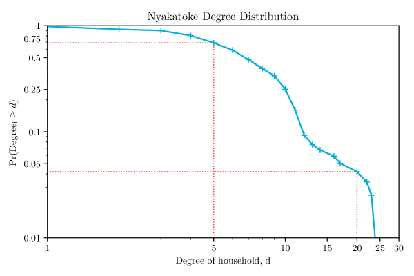
Figure 4: Nyakatoke Degree Distribution

Notes: This figure plots the probability (vertical axis) that a random household in Nyakatoke has strictly more risk sharing links than listed on the horizontal axis.

Source: De Weerdt, (2004) and authors’ calculations. Raw data available at https://www.uantwerpen.be/en/staff/joachim-deweerdt/ (Accessed January 2017).

Figure 5 displays estimates of the distribution of two star and triangle counts, as well as the transitivity index (and “optimal” transitivity statistic), with respect to the distribution of uniform draws from $\mathbb{D}_{N,\mathbf{d}_{+}}$ ($N=119$ and $\mathbf{d}_{+}$ coinciding with the one observed in Nyakatoke). Measured transitivity is Nyakatoke is extreme relative to this reference distribution. This suggests that clustering of links is, in fact, a special feature of the Nyakatoke network. It is also interesting to note that the distribution of transitivity in this reference distribution is well to the right of 0.0698 (the density of all graphs in the reference distribution). The skewed degree distribution in Nyakatoke forces a certain amount of transitivity, since high degree nodes are more likely to link with one another. This highlights the value of a test which proceeds conditionally on the degree sequence.

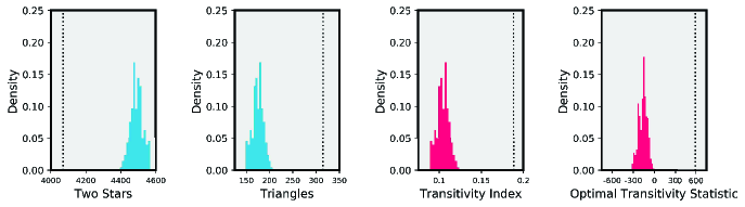
Figure 5: Reference distribution of transitivity index for Nyakatoke network

Notes: Histogram of two star counts, triangle counts and transitivity index values across 5,000 draws from $\mathbb{D}_{N,\mathbf{d}_{+}}$ ($N=119$ and $\mathbf{d}_{+}$coinciding with the one observed in Nyakatoke). The final figure plots the distribution of the “optimal” transitivity statistic given in Equation (13).

Sources: De Weerdt, (2004) and authors’ calculations. Raw data available at https://www.uantwerpen.be/en/staff/joachim-deweerdt/ (Accessed January 2017).

Figure 6 displays estimates of the distribution of network diameter and average distance. Nyakatoke’s diameter is not atypical across networks with the same degree sequence. However, average distance is significantly longer in Nyakatoke. One interpretation of this fact is that the Nyakatoke includes a distinct periphery of poorly connected/insured households.

Figure 6: Reference distribution of network diameter and average distance for Nyakatoke network

Notes: Histogram of values network diameter and average distance across 5,000 draws from $\mathbb{D}_{N,\mathbf{d}_{+}}$ ($N=119$ and $\mathbf{d}_{+}$coinciding with the one observed in Nyakatoke).

Sources: De Weerdt, (2004) and authors’ calculations. Raw data available at https://www.uantwerpen.be/en/staff/joachim-deweerdt/ (Accessed January 2017).

References

- Blitzstein & Diaconis, (2011) Blitzstein, J. & Diaconis, P. (2011). A sequential importance sampling algorithm for generating random graphs with prescribed degrees. Internet Mathematics, 6(4), 489 – 522.
- Bloch & Jackson, (2006) Bloch, F. & Jackson, M. O. (2006). Definitions of equilibrium in network formation games. International Journal of Game Theory, 34(3), 305 – 318.
- Bloch & Jackson, (2007) Bloch, F. & Jackson, M. O. (2007). The formation of networks with transfers among players. Journal of Economic Theory, 113(1), 83 – 110.
- Chatterjee et al., (2011) Chatterjee, S., Diaconis, P., & Sly, A. (2011). Random graphs with a given degree sequence. Annals of Applied Probability, 21(4), 1400 – 1435.
- Comola & Fafchamps, (2014) Comola, M. & Fafchamps, M. (2014). Testing unilateral and bilateral link formation. Economic Journal, 124(579), 954 – 976.
- Cox, (2006) Cox, D. R. (2006). Principles of Statistical Inference. Cambridge: Cambridge University Press.
- De Weerdt, (2004) De Weerdt, J. (2004). Insurance Against Poverty, chapter Risk-sharing and endogenous network formation, (pp. 197 – 216). Oxford University Press: Oxford.
- Del Genio et al., (2010) Del Genio, C. I., Kim, H., Toroczkai, Z., & Bassler, K. (2010). Efficient and exact sampling of simple graphs with given arbitrary degree sequence. Plos One, 5(4), e100012.
- Erdös et al., (2010) Erdös, P. L., Mikos, I., & Toroczkai, Z. (2010). A simple havel-hakimi type algorithm to realize graphical degree sequences of directed graphs. Electronic Journal of Combinatorics, 17(1), R66.
- Ferguson, (1967) Ferguson, T. S. (1967). Mathematical Statistics: A Decision Theoretic Approach. New York: Academic Press.
- Fisher, (1935) Fisher, R. A. (1935). The Design of Experiments. Edinburgh: Oliver and Boyd.
- Graham, (2016) Graham, B. S. (2016). Homophily and transitivity in dynamic network formation. NBER Working Paper 22186, National Bureau of Economic Research.
- Graham, (2017) Graham, B. S. (2017). An econometric model of network formation with degree heterogeneity. Econometrica, 85(4), 1033 – 1063.
- Hakimi, (1962) Hakimi, S. L. (1962). On realizability of a set of integers as degrees of the vertices of a linear graph. i. Journal of the Society for Industrial and Applied Mathematics, 10(3), 496 – 506.
- Havel, (1955) Havel, V. J. (1955). A remark on the existence of finite graph. Časopis Pro Pěstování Matematiky, 80, 477 – 480.
- Jackson, (2008) Jackson, M. O. (2008). Social and Economic Networks. Princeton: Princeton University Press.
- Jackson et al., (2012) Jackson, M. O., Rodriguez-Barraquer, T., & Tan, X. (2012). Social capital and social quilts: network patterns of favor exchange. American Economic Review, 102(5), 1857–1897.
- Kim et al., (2012) Kim, H., Del Genio, C. I., Bassler, K. E., & Toroczkai, Z. (2012). Constructing and sampling directed graphs with given degree sequences. New Journal of Physics, 14, 023012.
- Lehmann & Romano, (2005) Lehmann, E. L. & Romano, J. P. (2005). Testing Statistical Hypotheses. New York: Springer, 3rd edition.
- McDonald et al., (2007) McDonald, J. W., Smith, P. W. F., & Forster, J. J. (2007). Markov chain monte carlo exact inference for social networks. Social Networks, 29(1), 127 – 136.
- McPherson et al., (2001) McPherson, M., Smith-Lovin, L., & Cook, J. M. (2001). Birds of a feather: homophily in social networks. Annual Review of Sociology, 27(1), 415 – 444.
- Milo et al., (2002) Milo, R., Shen-Orr, S., Itzkovitz, S., Kashtan, N., Chklovskii, D., & Alon, U. (2002). Network motifs: simple building blocks of complex networks. Science, 298(5594), 824 – 827.
- Miyauchi, (2016) Miyauchi, Y. (2016). Structural estimation of a pairwise stable network with nonnegative externality. Journal of Econometrics, 195(2), 224 – 235.
- Moreira, (2009) Moreira, M. J. (2009). Tests with correct size when instruments can be arbitrarily weak. Journal of Econometrics, 152(2), 131-140, 152(2), 131 – 140.
- Owen, (2013) Owen, A. B. (2013). Monte carlo theory, methods and examples. Book Manuscript.
- Pelican & Graham, (2019) Pelican, A. & Graham, B. S. (2019). Testing for strategic interaction in social and economic network formation. Technical report, University of California - Berkeley.
- Rao et al., (1996) Rao, A. R., Jana, R., & Bandyopadhyay, S. (1996). A markov chain monte carlo method for generating random (0,1)-matrices with given marginals. Sankhya, 58(2), 225 – 242.
- Sierksma & Hoogeveen, (1991) Sierksma, G. & Hoogeveen, H. (1991). Seven criteria for integer sequences being graphic. Journal of Graph Theory, 15(2), 223 – 231.
- Snijders, (1991) Snijders, T. A. B. (1991). Enumeration and simulation methods for 0-1 matrices with given marginals. Psychometrika, 56(3), 397 – 417.
- Tarski, (1955) Tarski, A. (1955). A lattice-theoretical fixpoint theorem and its applications. Pacific Journal of Mathematics, 5(2), 285 – 309.
- Zhang & Chen, (2013) Zhang, J. & Chen, Y. (2013). Sampling for conditional inference on network data,. Journal of the American Statistical Association, 108(504), 1295 – 1307.