Adversarial Robustness Curves

Abstract

The existence of adversarial examples has led to considerable uncertainty regarding the trust one can justifiably put in predictions produced by automated systems. This uncertainty has, in turn, lead to considerable research effort in understanding adversarial robustness. In this work, we take first steps towards separating robustness analysis from the choice of robustness threshold and norm. We propose robustness curves as a more general view of the robustness behavior of a model and investigate under which circumstances they can qualitatively depend on the chosen norm.

1 Introduction

Robustness of machine learning models has recently attracted massive research interest. This interest is particularly pronounced in the context of deep learning. On the one hand, this is due to the massive success and widespread deployment of deep learning. On the other hand, it is due to the intriguing properties that can be demonstrated for deep learning (although these are not unique to this setting): the circumstance that deep learning can produce models that achieve or surpass human-level performance in a wide variety of tasks, but completely disagree with human judgment after application of imperceptible perturbations [1]. The ability of a classifier to maintain its performance under such changes to the input data is commonly referred to as robustness to adversarial perturbations.

In order to better understand adversarial robustness, recent years have seen the development of a host of methods that produce adversarial examples, in the white box and black box settings, with specific or arbitrary target labels, and varying additional constraints [2, 3, 4, 5, 6]. There has also been a push towards training regimes that produce adversarially robust networks, such as data augmentation with adversarial examples or distillation [7, 8, 9, 10]. The difficulty faced by such approaches is that robustness is difficult to measure and quantify: even if a model is shown to be robust against current state of the art attacks, this does not exclude the possibility that newly devised attacks may be successful [11]. The complexity of deep learning models and counter-intuitive nature of some phenomena surrounding adversarial examples further make it challenging to understand the impact of robust training or the properties that determine whether a model is robust or non-robust. Recent work has highlighted settings where no model can be simultaneously accurate and robust [12], or where finding a model that is simultaneously robust and accurate requires optimizing over a different hypothesis class than finding one that is simply accurate [13]. These examples rely on linear models, as they are easy for humans to understand. They analyze robustness properties for a fixed choice of norm and, typically, a fixed disadvantageous perturbation size (dependent on the model). This raises the question: “How do the presented results depend on the choice of norm, choice of perturbation size, and choice of linear classifier as a hypothesis class?”

In this contribution, we:

• propose robustness curves as a way of better representing adversarial robustness in place of “point-wise” measures,

• show that linear classifiers are not sufficient to illustrate all interesting robustness phenomena, and

• investigate how robustness curves may depend on the choice of norm.

2 Definitions

In the following, we assume data $(x,y)\in X\times Y$, $X\subseteq\mathbb{R}^{d}$, are generated i.i.d. according to distribution $P$ with marginal $P_{X}$. Let $f:X\to Y$ denote some classifier and let $x\in X$. The standard loss of $f$ on $P$ is

$$L(f):=P(\{(x,y):f(x)\neq y\})\,.$$ (1)

Let $n:X\to\mathbb{R}^{+}$ be some norm, let $\varepsilon\geq 0$ and let

$$B_{n}(x,\varepsilon):=\{x^{\prime}:n(x-x^{\prime})\leq\varepsilon\}\,.$$ (2)

Following [12], we define the $\varepsilon$-adversarial loss of $f$ regarding $P$ and $n$ as

$$L_{n,\varepsilon}(f):=P(\underbrace{\{(x,y):\exists x^{\prime}\in B_{n}(x,\varepsilon):f(x^{\prime})\neq y\}}_{=:A_{\varepsilon}^{n}})\,.$$ (3)

We have $L_{n,0}(f)=L(f)$. Alternatively, we can exclude from this definition any points that are initially misclassified by the model, and instead consider as adversarial examples all points where the model changes its behavior under small perturbations. Then the $\varepsilon$-margin loss is defined as

$$L^{\prime}_{n,\varepsilon}(f):=P_{X}(\{x:\exists x^{\prime}\in B_{n}(x,\varepsilon):f(x^{\prime})\neq f(x)\})\,.$$ (4)

$L^{\prime}_{n,\varepsilon}$ is the weight of all points within an $\varepsilon$-margin of a decision boundary. We have $L^{\prime}_{n,0}(f)=0$.

There are two somewhat arbitrary choices in the definition in Equations 3 and 4: the choice of $\varepsilon$ and the choice of the norm $n$. The aim of this contribution is to investigate how $\varepsilon$ and $n$ impact the adversarial robustness.

3 Robustness Curves

As a first step towards understanding robustness globally, instead of for an isolated perturbation size $\varepsilon$, we propose to view robustness as a function of $\varepsilon$. This yields an easy-to-understand visual representation of adversarial robustness in the form of a robustness curve.

Definition 1

The robustness curve of a classifier $f$, given a norm $n$ and underlying distribution $P$, is the curve defined by

$$r_{f,n,P}:[0,\infty) \to[0,1]$$ (5)

$$\varepsilon \mapsto L_{n,\varepsilon}(f)\,.$$ (6)

The margin curve of $f$ given $n$ and $P$ is the curve defined by

$$r^{\prime}_{f,n,P}:[0,\infty) \to[0,1]$$ (7)

$$\varepsilon \mapsto L^{\prime}_{n,\varepsilon}(f)\,.$$ (8)

Commonly chosen norms for the investigation of adversarial robustness are the $\ell_{1}$ norm (denoted by $\|\cdot\|_{1}$), the $\ell_{2}$ norm (denoted by $\|\cdot\|_{2}$), and the $\ell_{\infty}$ norm (denoted by $\|\cdot\|_{\infty}$). In the following, we will investigate robustness curves for these three choices of $n$.

[12] propose a distribution $P_{1}$ where $y\stackrel{{\scriptstyle\text{u.\,a.\,r.\@}}}{{\sim}}\{-1,+1\}$ and

$$x_{1}=\begin{cases}1&\text{w.\,p.\@}\,p\\ -1&\text{w.\,p.\@}\,(1-p)\end{cases}\quad x_{2},\dots,x_{d+1}\stackrel{{\scriptstyle\text{i.\,i.\,d.\@}}}{{\sim}}\mathcal{N}(\eta y,1).$$ (9)

For this distribution, they show that the linear classifier $f_{\mathrm{avg}}(x)=\operatorname{sign}(w^{T}x)$ with $w=(0,1/d,\dots,1/d)$ has high accuracy, but low $\varepsilon$-robustness in $\ell_{\infty}$ norm for $\varepsilon\geq 2\eta$, while the classifier $f_{\mathrm{rob}}(x)=\operatorname{sign}(w^{T}x)$ with $w=(1,0,\dots,0)$ has high $\varepsilon$-robustness for $\varepsilon<1$, but low accuracy. [13] proposes a distribution $P_{2}$ where $y\stackrel{{\scriptstyle\text{u.\,a.\,r.\@}}}{{\sim}}\{-1,+1\}$ and

$$x_{i}=\begin{cases}y&\text{w.\,p.\@}\,0.51\\ -y&\text{w.\,p.\@}\,0.49\end{cases}$$ (10)

where the linear classifier $f_{s}(x)=\operatorname{sign}(w^{T}x)$ with $w=\vec{1}_{d}$ has high accuracy, but low $\varepsilon$-robustness in $\ell_{\infty}$ norm for $\varepsilon\geq\frac{1}{2}$. Figure 1 shows margin curves and robustness curves for $P_{1}$ and $f_{\mathrm{avg}}$, $P_{1}$ and $f_{\mathrm{rob}}$ and $P_{2}$ and $f_{s}$.

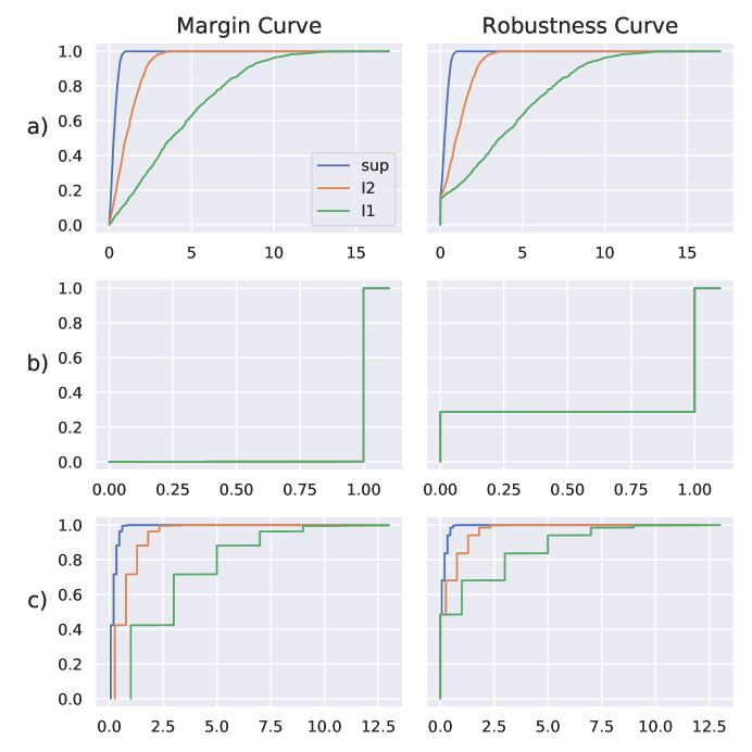
Figure 1: Margin curves and robustness curves for several examples of distributions and linear models from the literature. Row a) shows curves for classifier $f_{\mathrm{avg}}$ and distribution $P_{1}$. Row b) shows curves for classifier $f_{\mathrm{rob}}$ and distribution $P_{1}$. In this case, all three curves are identical and thus appear as one. Row c) shows curves for classifier $f_{s}$ and distribution $P_{2}$.

4 The impact of $n$

The curves shown in Figure 1 seem to behave similarly for each norm. Is this always the case? Indeed, if $f$ is a linear classifier parameterized by normal vector $w$ and offset $b$, denote by

$$d_{n}((w,b),x)=\min\{n(v):\exists p:x=p+v,\langle w,p\rangle+b=0\}$$ (11)

the shortest distance between $(w,b)$ and $x$ in norm $n$. Then a series of algebraic manipulations yield

$$d_{\|\cdot\|_{1}}((w,b),x) =\frac{|b+\langle w,x\rangle|}{\|w\|_{\infty}}\,,$$ (12)

$$d_{\|\cdot\|_{2}}((w,b),x) =\frac{|b+\langle w,x\rangle|}{\|w\|_{2}}\,,$$ (13)

$$d_{\|\cdot\|_{\infty}}((w,b),x) =\frac{|b+\langle w,x\rangle|}{\|w\|_{1}}\,.$$ (14)

In particular, there exist constants $c$ and $c^{\prime}$ depending on $(w,b)$ such that for all $x\in X$,

$$d_{\|\cdot\|_{1}}((w,b),x)=cd_{\|\cdot\|_{2}}((w,b),x)=c^{\prime}d_{\|\cdot\|_{\infty}}((w,b),x)$$ (15)

This implies the following Theorem:

Theorem 1

For any linear classifier $f$, there exist constants $c,c^{\prime}>0$ such that for any $\varepsilon\geq 0$,

$$L_{\|\cdot\|_{1},\varepsilon}(f)=L_{\|\cdot\|_{2},\varepsilon/c}(f)=L_{\|\cdot\|_{\infty},\varepsilon/c^{\prime}}(f)\,.$$ (16)

As a consequence, for linear classifiers, dependence of robustness curves on the choice of norm is purely a matter of compression and elongation.

What can we say about classifiers with more complex decision boundaries? For all $x$, we have

$$\|x\|_{\infty}\leq\|x\|_{2}\leq\|x\|_{1}\leq\sqrt{d}\|x\|_{2}\leq d\|x\|_{\infty}\,.$$ (17)

These inequalities are tight, i.e. there for each inequality there exists some $x$ such that equality holds. It follows that, for any $\varepsilon>0$,

$$A_{\varepsilon/d}^{\|\cdot\|_{\infty}}\subseteq A_{\varepsilon/\sqrt{d}}^{\|\cdot\|_{2}}\subseteq A_{\varepsilon}^{\|\cdot\|_{1}}\subseteq A_{\varepsilon}^{\|\cdot\|_{2}}\subseteq A_{\varepsilon}^{\|\cdot\|_{\infty}}$$ (18)

and so

$$L_{\|\cdot\|_{\infty},\varepsilon}(f) \geq L_{\|\cdot\|_{2},\varepsilon}(f)\geq L_{\|\cdot\|_{1},\varepsilon}(f)$$ (19)

$$\geq L_{\|\cdot\|_{2},\varepsilon/\sqrt{d}}(f)\geq L_{\|\cdot\|_{1},\varepsilon/d}(f)\,.$$ (20)

In particular, the robustness curve for the $\ell_{\infty}$-norm is always an upper bound for the robustness curve for any other $\ell_{p}$-norm (since $\|x\|_{p}\leq\|x\|_{\infty}$ for all $x$ and $p\geq 1$). Thus, for linear classifiers as well as classifiers with more complicated decision boundaries, in order to show that a model is adversarially robust for any fixed norm, it is sufficient to show that it exhibits the desired robustness behavior for the $\ell_{\infty}$-norm. On the other hand, in order to show that a model is not adversarially robust, showing this for the $\ell_{\infty}$ norm does not necessarily imply the same qualities in another norm, as the robustness curves may be strongly separated in high-dimensional spaces, both for linear and non-linear models.

Contrary to linear models, for more complicated decision boundaries, robustness curves may also exhibit qualitatively different behavior. This is illustrated in Figure 2. The decision boundary in each case is given by a quadratic model in 2-dimensional space: $f(\vec{x})=\operatorname{sign}(x_{1}^{2}-x_{2})$. In the first example, we construct a finite set of points, all at $\ell_{2}$-distance 1 from the decision boundary, but at various $\ell_{1}$ and $\ell_{\infty}$ distances. For any distribution concentrated on a set of such points, the $\ell_{2}$-robustness curve jumps from zero to one at a single threshold value, while the $\ell_{1}$- and $\ell_{\infty}$-robustness curves are step functions with the height of the steps determined by the distribution across the points and the width determined by the variation in $\ell_{1}$ or $\ell_{\infty}$ distances from the decision boundary. The robustness curves in this example also exhibit, at some points, the maximal possible separation by a factor of $\sqrt{d}$ (note that $d=2$) while touching in other points. In the second example, we show a continuous version of the same phenomenon, with points inside and outside the parabola distributed at constant $\ell_{2}$-distance from the decision boundary, but with varying $\ell_{1}$ and $\ell_{\infty}$ distances. As a result, the robustness curves for different norms are qualitatively different. The third example, on the other hand, shows a setting where the robustness curves for the three norms are both quantitatively and qualitatively similar.

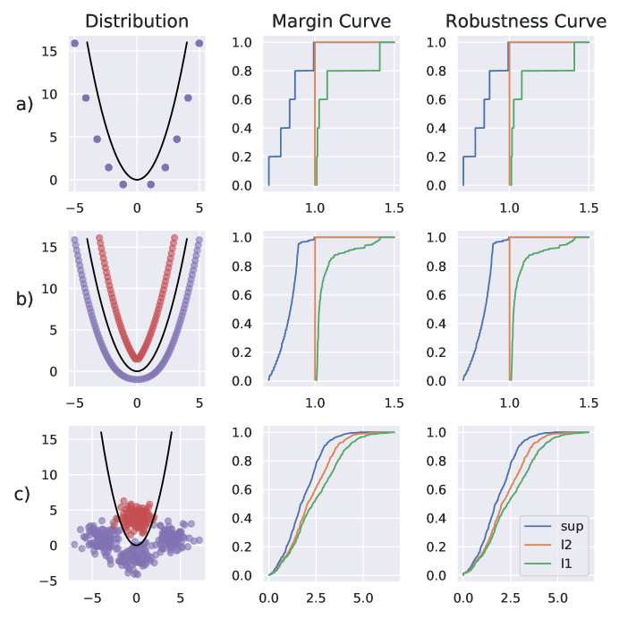
Figure 2: Margin curves and robustness curves for $f(\vec{x})=\operatorname{sign}(x_{1}^{2}-x_{2})$ and three different underlying distributions, illustrating varying behavior of the robustness curves for different norms. In rows a) and b), the robustness curves are qualitatively different, while they are almost identical in row c). Note that in these examples, robustness curves and margin curves are nearly identical, as the standard loss of $f$ is zero or close to zero in all cases.

These examples drive home two points:

• The robustness properties of a classifier may depend both quantitatively and qualitatively on the norm chosen to measure said robustness. When investigating robustness, it is therefore imperative to consider which norm, or, more broadly, which concept of closeness best represents the type of perturbation to guard against.

• Linear classifiers are not a sufficient tool for understanding adversarial robustness in general, as they in effect neutralize a degree of freedom given by the choice of norm.

5 Discussion

We have proposed robustness curves as a more general perspective on the robustness properties of a classifier and have discussed how these curves can or cannot be affected by the choice of norm. Robustness curves are a tool for a more principled investigation of adversarial robustness, while their dependence on a chosen norm underscores the necessity of basing robustness analyses on a clear problem definition that specifies what kind of perturbations a model should be robust to. We note that the use of $\ell_{p}$ norms in current research is frequently meant only as an approximation of a “human perception distance” [14]. A human’s ability to detect a perturbation depends on the point the perturbation is applied to, meaning that human perception distance is not a homogeneous metric, and thus not induced by a norm. In this sense, where adversarial robustness is meant to describe how faithful the behavior of a model matches that of a human, the adversarial loss in Equation 3 can only be seen as a starting point of analysis. Nonetheless, since perturbations with small $\ell_{p}$-norm are frequently imperceptible to humans, adversarial robustness regarding some $\ell_{p}$-norm is a reasonable lower bound for adversarial robustness in human perception distance. In future work, we would like to investigate how robustness curves can be estimated for deep networks and extend the definition to robustness against targeted attacks.

References

- [1] Christian Szegedy, Wojciech Zaremba, Ilya Sutskever, Joan Bruna, Dumitru Erhan, Ian J. Goodfellow and Rob Fergus “Intriguing properties of neural networks”, 2014 arXiv:1312.6199
- [2] Ian J. Goodfellow, Jonathon Shlens and Christian Szegedy “Explaining and Harnessing Adversarial Examples”, 2014 arXiv:1412.6572
- [3] Alexey Kurakin, Ian J. Goodfellow and Samy Bengio “Adversarial examples in the physical world”, 2016 arXiv:1607.02533
- [4] Alexey Kurakin, Ian J. Goodfellow and Samy Bengio “Adversarial Machine Learning at Scale”, 2016 arXiv:1611.01236
- [5] Nicolas Papernot, Patrick D. McDaniel, Ian J. Goodfellow, Somesh Jha, Z. Celik and Ananthram Swami “Practical Black-Box Attacks against Deep Learning Systems using Adversarial Examples”, 2016 arXiv:1602.02697
- [6] Jiawei Su, Danilo Vasconcellos Vargas and Kouichi Sakurai “One pixel attack for fooling deep neural networks”, 2017 DOI: 10.1109/tevc.2019.2890858
- [7] Nicolas Papernot, Patrick McDaniel, Xi Wu, Somesh Jha and Ananthram Swami “Distillation as a Defense to Adversarial Perturbations Against Deep Neural Networks” In 2016 IEEE Symposium on Security and Privacy (SP) IEEE, 2016 DOI: 10.1109/sp.2016.41
- [8] Shixiang Gu and Luca Rigazio “Towards Deep Neural Network Architectures Robust to Adversarial Examples”, 2014 arXiv:1412.5068 [cs.LG]
- [9] Ruitong Huang, Bing Xu, Dale Schuurmans and Csaba Szepesvari “Learning with a Strong Adversary”, 2015 arXiv:1511.03034 [cs.LG]
- [10] Osbert Bastani, Yani Ioannou, Leonidas Lampropoulos, Dimitrios Vytiniotis, Aditya Nori and Antonio Criminisi “Measuring Neural Net Robustness with Constraints”, 2016 arXiv:1605.07262 [cs.LG]
- [11] Nicholas Carlini and David A. Wagner “Towards Evaluating the Robustness of Neural Networks” In 2017 IEEE Symposium on Security and Privacy (SP), 2017, pp. 39–57 DOI: 10.1109/sp.2017.49
- [12] Dimitris Tsipras, Shibani Santurkar, Logan Engstrom, Alexander Turner and Aleksander Madry “Robustness May Be at Odds with Accuracy” In International Conference on Learning Representations, 2019 URL: https://openreview.net/forum?id=SyxAb30cY7
- [13] Preetum Nakkiran “Adversarial Robustness May Be at Odds With Simplicity”, 2019 arXiv:1901.00532
- [14] Jan Philip Göpfert, Heiko Wersing and Barbara Hammer “Adversarial attacks hidden in plain sight”, 2019 arXiv:1902.09286