Dynamic Information Design with
Diminishing Sensitivity Over News

Abstract

A Bayesian agent experiences gain-loss utility each period over changes in belief about future consumption (“news utility”), with diminishing sensitivity over the magnitude of news. Diminishing sensitivity induces a preference over news skewness: gradual bad news, one-shot good news is worse than one-shot resolution, which is in turn worse than gradual good news, one-shot bad news. So, the agent’s preference between gradual information and one-shot resolution can depend on his consumption ranking of different states. In a dynamic cheap-talk framework where a benevolent sender communicates the state over multiple periods, the babbling equilibrium is essentially unique without loss aversion. More loss-averse agents may enjoy higher news utility in equilibrium, contrary to the commitment case. We characterize the family of gradual good news equilibria that exist with high enough loss aversion, and find the sender conveys progressively larger pieces of good news. We discuss applications to media competition and game shows.

Keywords: diminishing sensitivity, news utility, dynamic information design, cheap talk, preference over skewness of information

1 Introduction

People are sometimes willing to pay a cost to change how they receive news over time, even when the information does not help them make better decisions. Consider the following scenario:

Ann interviews for her dream job and is told that she will receive the decision by email next week. Ann knows that if the firm decides to reject her, she will receive the rejection email next Friday. But if the firm decides to hire her, she could hear back on any of the weekdays — in other words, no news is bad news. To avoid experiencing multiple instances of disappointment over the week in case she does not hear back for several days, Ann sets up an email filter to automatically redirect any emails from the firm into a holding tank, then releases all messages from the holding tank into her inbox at 5PM next Friday.

In this scenario, Ann may be willing to exert costly effort to modify her informational environment because she experiences diminishingly sensitive psychological reactions to good and bad news. She is elated by good news and disappointed by bad news in every period, and multiple congruent pieces of news carry a greater total emotional impact if they are experienced separately in different periods than if the aggregated lump-sum news arrives in a single period. This kind of psychological consideration also influences how people convey news to others. When CEOs announce earnings forecasts to shareholders and when organization leaders update their teams about recent developments, they are surely mindful of their information’s emotional impact (in addition to its possible instrumental value). Finally, the psychological effects of news also play a prominent role in designing entertainment content like game shows, where the audience experiences positive and negative reactions over time to news and developments that have no bearing on their personal decision-making.

In this paper, we study the implications of diminishingly sensitive reactions to news for informational preference and dynamic communication. A person’s future consumption depends on an unknown state of the world. In each period, he observes some information about the state and experiences gain-loss utility over the change in his belief about said future consumption (“news utility”). How does this person prefer to learn about the state over time? If there is another agent who knows the state and who wants to maximize the first person’s expected welfare, how will this informed agent communicate her information?

Of course, we are not the first to model news utility (see Kőszegi and Rabin (2009)) or to study psychological considerations in dynamic games (see the survey Battigalli and Dufwenberg (2022), for example). Our main innovation is the focus on the implications of diminishing sensitivity — a classical but surprisingly under-studied assumption. Diminishing sensitivity in reference dependence traces back to Kahneman and Tversky (1979)’s original formulation of prospect theory. Based on Weber’s law and experimental findings about human perception, these authors envisioned a gain-loss utility based on deviations from a reference point, where larger deviations carry smaller marginal effects. But almost all subsequent work on reference-dependent preferences use two-part linear gain-loss utility functions, so their results are driven by loss aversion but not diminishing sensitivity. Four decades since Kahneman and Tversky (1979)’s publication, O’Donoghue and Sprenger (2018)’s review of the ensuing literature summarizes the situation:

“Most applications of reference-dependent preferences focus entirely on loss aversion, and ignore the possibility of diminishing sensitivity […] The literature still needs to develop a better sense of when diminishing sensitivity is important.”

We show that diminishing sensitivity leads to novel and testable predictions for information design. First, when the agent commits to an information structure ex-ante, diminishing sensitivity generates a preference over the direction of news skewness. Any information structure where good news arrives all at once but bad news arrives gradually in small pieces — such as waiting for the job offer in Ann’s scenario — is strictly worse than resolving all uncertainty in one period (“one-shot resolution”). On the other hand, any information structure with the opposite skewness — good news arrives gradually but bad news all at once — is strictly better than one-shot resolution, provided loss aversion is weak enough. We relate this result to recent experiments about preference over the skewness of information in Section 5.1.

As Kőszegi and Rabin (2009) point out, the two-part linear news-utility model (without diminishing sensitivity) predicts that people prefer one-shot resolution over any other dynamic information structure. At the same time, some other theories (e.g., Ely, Frankel, and Kamenica (2015)’s suspense and surprise utility) make the “opposite” prediction that one-shot resolution is the worst possible information structure. By contrast, the skewness preference induced by news utility with diminishing sensitivity implies the same person can make different choices between gradual information and one-shot resolution in different situations — in particular, it depends on his consumption ranking over the states.

For instance, in a world where two possible states ($A$ and $B$) are associated with two different consumption prizes, imagine state $A$ realizes if and only if a sequence of intermediate events all take place successfully over time. We show that when the agent prefers the prize in state $A$, he will choose to observe the intermediate events resolve in real-time. But when he prefers the prize in state $B$, he will choose to only learn the final state. At the population level, this result shows that an underlying diversity in consumption preferences within a society can create a diversity in informational preferences, and suggests a mechanism for media competition. The result also rationalizes a “sudden death” format often found in game shows, where the contestant must overcome every challenge in a sequence to win the grand prize (as opposed to the grand prize being contingent on beating at least one of several challenges.)

Our second main result is that when an informed benevolent sender communicates the state to the receiver through cheap talk, the receiver’s diminishing sensitivity leads to credibility problems for the sender. We show that if the receiver has diminishing sensitivity and low enough loss aversion, the lack-of-commitment problem is so severe that every equilibrium is payoff-equivalent to the babbling equilibrium. The reason is that the sender strictly prefers to lie and say the state is good even when it is bad. This temptation is driven by the receiver’s diminishing sensitivity: even though the sender is far-sighted and knows false hope creates additional disappointment when the state is revealed, diminishing sensitivity limits the incremental disutility of this extra future disappointment. Diminishing sensitivity thus drives a wedge between the commitment solution and the equilibrium outcome, whereas the two coincide without it. We also show that high enough loss aversion can restore the equilibrium credibility of good-news messages by increasing the future disappointment cost of false hope in the bad state. As a consequence, receivers with higher loss aversion may enjoy higher equilibrium payoffs.

With enough loss aversion, there exist non-babbling equilibria featuring gradual good news. We characterize the entire family of such equilibria and study how quickly the receiver learns the state. For a class of news-utility functions that include a tractable quadratic specification, the sender always conveys progressively larger pieces of good news over time, so the receiver’s equilibrium belief grows at an increasing rate in the good state. The idea is that in equilibrium, the sender must be made indifferent between giving false hope and telling the truth in the bad state, and diminishing sensitivity implies that sustaining said indifference requires a greater amount of false hope when the receiver’s current belief is more optimistic. This conclusion also puts a uniform bound on the number of periods of informative communication across all time horizons and all equilibria.

The rest of the paper is organized as follows. Section 2 defines the timing of events and introduces a model of news utility with diminishing sensitivity. Section 3 studies how diminishing sensitivity leads to a preference over information structures with different skewness, then applies this result to show how an agent’s choice between gradual information and one-shot resolution depends on his consumption ranking of the states. Section 4 considers an environment where an informed benevolent sender communicates the state to a receiver with news utility, and focuses on the credibility problems in the resulting cheap-talk game. Section 5 discusses related literature and contrasts our results with the predictions of other models of preference over non-instrumental information. Section 6 concludes.

2 Model

2.1 Timing of Events

We consider a discrete-time model with periods $0,1,2,...,$$T$, where $T\geq 2$. There is a binary state space $\Theta=\{A,B\}.$ In the final period $T,$ the agent receives a state-dependent consumption prize $c_{\theta}$ and derives consumption utility $v(c_{\theta})\in\mathbb{R}$. There is no consumption in other periods, and we assume that $v(c_{A})\neq v(c_{B}).$ We may normalize $v$ without loss so that the agent gets consumption utility 1 in one state and 0 in the other.

The agent starts with a prior probability $0<\pi_{0}<1$ of the state being $A$. In every period $t=1,...,T,$ the agent observes some information and updates his belief about $\{\theta=A\}$ to the Bayesian posterior $0\leq\pi_{t}\leq 1.$ The information is non-instrumental in that no actions taken in these interim periods affect the state or the consumption utility in period $T$. In period $T,$ he exogenously and perfectly learns the true state $\theta$ at the moment of consumption, so we always have $\pi_{T}=1$ if $\theta=A$ and $\pi_{T}=0$ if $\theta=B$.

2.2 News Utility

Although the agent only consumes in the final period, he experiences news utility over consumption in every period. He has a gain-loss utility function, $\mu:[-1,1]\to\mathbb{R}$, that maps changes in expected final-period consumption utility into a felicity level. Let $\rho_{t}=\sum_{\theta\in\Theta}\pi_{t}(\theta)v(c_{\theta})$ denote this expectation based on the agent’s belief in period $t$, and note $\rho_{t}\in[0,1]$ based on our normalization of $v.$ At the end of period $1\leq t\leq T,$ the agent experiences news utility $\mu(\rho_{t}-\rho_{t-1})$ — that is, he derives joy or pain based on the recent belief update from $\pi_{t-1}$ to $\pi_{t}.$ Utility flow is undiscounted and the agent has the same $\mu$ in all periods, so his total payoff is $\sum_{t=1}^{T}\mu(\rho_{t}-\rho_{t-1})+v(c).$

Throughout we assume $\mu$ is continuous, strictly increasing, twice differentiable except possibly at 0, and $\mu(0)=0.$ We maintain further assumptions on $\mu$ to reflect diminishing sensitivity and loss aversion.

Definition 1.

Say $\mu$ satisfies diminishing sensitivity if $\mu^{{}^{\prime\prime}}(x)<0$ and $\mu^{{}^{\prime\prime}}(-x)>0$ for all $x>0.$ Say $\mu$ satisfies (weak) loss aversion if $-\mu(-x)\geq\mu(x)$ for all $x>0.$ There is strict loss aversion if $-\mu(-x)>\mu(x)$ for all $x>0.$

For instance, the gain-loss function $\mu$ in Tversky and Kahneman (1992) where $\mu(x)=x^{\alpha}$ for $x\geq 0,$ $\mu(x)=-\lambda|x|^{\beta}$ for $x<0$ with $0<\alpha,\beta<1$ and $\lambda>1$ satisfies both diminishing sensitivity and strict loss aversion.

This model of diminishing sensitivity over the magnitude of news shares the same psychological motivation as Kahneman and Tversky (1979), who base their theory of human responses to monetary gains and losses on Weber’s law and on psychology experiments about how people perceive changes in physical attributes like temperature or brightness. This framework of deriving utility from changes in beliefs has been previously discussed in Kőszegi and Rabin (2009), but they mostly focus on another model that makes percentile-by-percentile comparisons between old and new beliefs and without diminishing sensitivity. The model we use allows us to characterize the implications of diminishing sensitivity in the simplest setup with two states.

2.2.1 Quadratic News Utility

We discuss another tractable functional form of $\mu$ that is rich enough to exhibit both diminishing sensitivity and loss aversion. The quadratic news-utility function $\mu:[-1,1]\to\mathbb{R}$ is given by

$$\mu(x)=\begin{cases}\alpha_{p}x-\beta_{p}x^{2}&x\geq 0\\ \alpha_{n}x+\beta_{n}x^{2}&x<0\end{cases}$$

with $\alpha_{p},\beta_{p},\alpha_{n},\beta_{n}>0.$ So we have

$$\mu^{{}^{\prime}}(x)=\begin{cases}\alpha_{p}-2\beta_{p}x&x>0\\ \alpha_{n}+2\beta_{n}x&x<0\end{cases},\qquad\mu^{{}^{\prime\prime}}(x)=\begin{cases}-2\beta_{p}&x>0\\ 2\beta_{n}&x<0\end{cases}.$$

The parameters $\alpha_{p},\alpha_{n}$ control the extent of loss aversion near 0, while $\beta_{p},\beta_{n}$ determine the amount of curvature — i.e., the second derivative of $\mu$. The maintained general assumptions on $\mu$ imply the following parametric restrictions.

1. Monotonicity: $\alpha_{p}>2\beta_{p}$ and $\alpha_{n}>2\beta_{n}$. These inequalities hold if and only if $\mu$ is strictly increasing.

2. Loss aversion: $\alpha_{n}-\alpha_{p}\geq(\beta_{n}-\beta_{p})z$ for all $z\in[0,1]$. This condition is equivalent to loss aversion from Definition 1 for this class of news-utility functions.

A family of quadratic news-utility functions that satisfy these two restrictions can be constructed by choosing any $\alpha>2\beta>0$ and $\lambda\geq 1$, then set $\alpha_{p}=\alpha$, $\alpha_{n}=\lambda\alpha$, $\beta_{p}=\beta,$ $\beta_{n}=\lambda\beta$. Figure 1 plots some of these news-utility functions for different values of $\alpha,\beta,$ and $\lambda$.

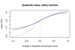
Figure 1: Examples of quadratic news-utility functions in the family $\alpha_{p}=\alpha$, $\alpha_{n}=\lambda\alpha$, $\beta_{p}=\beta,$ $\beta_{n}=\lambda\beta$. Grey curve: $\alpha=2,$ $\beta=1,$ $\lambda=1$. Red curve: $\alpha=2$, $\beta=1$, $\lambda=2$. Blue curve: $\alpha=2,$ $\beta=0.8$, $\lambda=1$.

3 Diminishing Sensitivity and Preference over News Skewness

In this section, we show that news utility with diminishing sensitivity makes novel predictions about preference over the skewness of information. When there is no loss aversion, one-shot resolution of uncertainty is neither the agent’s most preferred way to get information nor the least preferred. Instead, the agent strictly prefers one-shot resolution over an information structure that delivers piecemeal bad news over time, and strictly prefers an information structure with the opposite skewness over one-shot resolution. By continuity, the same conclusions hold when loss aversion is present but sufficiently weak.

Definition 2.

An information structure features gradual good news, one-shot bad news if

• $\mathbb{P}[\rho_{t}\geq\rho_{t-1}\text{ for all }1\leq t\leq T\mid\rho_{T}=1]=1$ and

• $\mathbb{P}[\rho_{t}<\rho_{t-1}\text{ for no more than one }1\leq t\leq T\mid\rho_{T}=0]=1$.

An information structure features gradual bad news, one-shot good news if

• $\mathbb{P}[\rho_{t}\leq\rho_{t-1}\text{ for all }1\leq t\leq T\mid\rho_{T}=0]=1$ and

• $\mathbb{P}[\rho_{t}>\rho_{t-1}\text{ for no more than one }1\leq t\leq T\mid\rho_{T}=1]=1$.

The event $\rho_{T}=1$ corresponds to the “good” state being realized and $\rho_{T}=0$ corresponds to the “bad” state being realized, from the perspective of the agent’s consumption utility. In the gradual good news, one-shot bad news information structures, the agent gets good news over time and gradually increases his expectation of future consumption. When the state is bad, the agent gets all the negative information at once — in the first period when his expectation $\rho_{t}$ strictly decreases, he fully learns that the state is bad. Conversely, “gradual bad news, one-shot good news” refers to the opposite kind of information structure.

An information structure features one-shot resolution if $\mathbb{P}[\rho_{t}\neq\rho_{t-1}\text{ for at most one }1\leq t\leq T]=1.$ That is, almost surely the agent’s belief only changes in one period (including the final period when true state is perfectly revealed). Note that one-shot resolution falls into both classes from Definition 2. We say that an information structure features strictly gradual good news if

$$\mathbb{P}[\rho_{t}>\rho_{t-1}\text{ and }\rho_{t^{{}^{\prime}}}>\rho_{t^{{}^{\prime}}-1}\text{ for two distinct }1\leq t,t^{{}^{\prime}}\leq T\mid\rho_{T}=1]>0.$$

That is, there is positive probability that the agent’s expectation strictly increases at least twice in periods $1$ through $T$. Similarly define strictly gradual bad news.

We now prove that whenever $\mu$ satisfies diminishing sensitivity and (weak) loss aversion, information structures featuring strictly gradual bad news, one-shot good news are strictly worse than one-shot resolution. The intuition is that information structures in this class deliver small pieces of bad news but large clumps of good news, which is the exact opposite of what the agent wants when he experiences diminishing sensitivity to news.

Proposition 1.

Suppose $\mu$ satisfies diminishing sensitivity and weak loss aversion. Any information structure featuring strictly gradual bad news, one-shot good news provides strictly lower utility than one-shot resolution in expectation, and almost surely weakly lower utility ex-post.

Proposition 1 identifies a class of information structures that are worse than one-shot resolution for news utility with diminishing sensitivity, distinguishing it from other models of information preference where one-shot resolution is the worst possible information structure. Utility models that make this other prediction include suspense and surprise (Ely, Frankel, and Kamenica, 2015) and news utility with a two-part linear, gain-loving (instead of loss-averse) value function (Chapman, Snowberg, Wang, and Camerer, 2022; Campos-Mercade, Goette, Graeber, Kellogg, and Sprenger, 2022).

Next, we show that if the agent has diminishing sensitivity but not loss aversion, then information structures with strictly gradual good news, one-shot bad news are strictly better than one-shot resolution.

Proposition 2.

Suppose $\mu$ satisfies diminishing sensitivity and it is symmetric around 0 with $-\mu(-x)=\mu(x)$ for all $x\geq 0$ (that is, it does not exhibit loss aversion). Any information structure featuring strictly gradual good news, one-shot bad news provides strictly higher utility than one-shot resolution in expectation, and almost surely weakly higher utility ex-post.

In Kőszegi and Rabin (2009)’s model of news utility without diminishing sensitivity, one-shot resolution is optimal among all information structures. By contrast, Proposition 2 can be combined with continuity to show that for news-utility functions with diminishing sensitivity and a small enough amount of loss aversion, there are information structures that are strictly better than one-shot resolution. To make this precise, consider the parametric class of $\lambda$-scaled news-utility functions. We fix some $\tilde{\mu}_{pos}:[0,1]\to\mathbb{R}_{+}$, strictly increasing and strictly concave with $\tilde{\mu}_{pos}(0)=0$, and consider the family of news-utility functions given by $\mu_{\lambda}(x)=\tilde{\mu}_{pos}(x)$, $\mu_{\lambda}(-x)=-\lambda\tilde{\mu}_{pos}(x)$ for $x>0$ as we vary the loss aversion parameter $\lambda\geq 1.$

Corollary 1.

Consider a class of $\lambda$-scaled news-utility functions $(\mu_{\lambda})_{\lambda\geq 1}$ and any information structure featuring strictly gradual good news, one-shot bad news. There exists some $\bar{\lambda}>1$ so that for any $1\leq\lambda\leq\bar{\lambda}$, this information structure gives strictly higher utility than one-shot resolution in expectation.

In summary, provided loss aversion is low enough, diminishing sensitivity induces the following preference ranking: gradual good news, one-shot bad news is better than one-shot resolution, which is in turn better than gradual bad news, one-shot good news. Section 5.1 discusses related experimental literature about preference over news skewness, and Appendix B contains additional results about preference over information structures.

3.1 Consumption Preference and Information Preference

An an application, we consider an environment where a sequence of signal realizations gradually determine the binary state. We show that agents with opposite consumption preferences over the two states can exhibit opposite preferences between observing the signals as they arrive or only learning the final state, because the same gradual information translates into two different kinds of skewness for these agents.

In each period $t=1,2,...,T$, a binary signal $X_{t}$ realizes, where $\mathbb{P}[X_{t}=1]=q_{t}$ with $0<q_{t}<1$. Each $X_{t}$ is independent of the other ones. The signals determine the state. If $X_{t}=1$ for all $t$, then the state is $A$. Otherwise, when $X_{t}=0$ for at least one $t$, the state is $B$. At time 0, the agent chooses between observing the realizations of the signals $(X_{t})_{t=1}^{T}$ in real time (gradual information), or only learning the state of the world at the end of period $T$ (one-shot resolution).

For a concrete example, imagine a televised debate between two political candidates $A$ and $B$ where $A$ loses as soon as she makes a “gaffe” during the debate. If $A$ does not make any gaffes, then $A$ wins. In this example, $\{X_{t}=1\}$ corresponds to the event that candidate $A$ does not make a gaffe during the $t$-th minute of the debate. States $A$ and $B$ correspond to candidates $A$ and $B$ winning the debate. An individual chooses between watching the debate live (i.e., observing the stochastic process $(X_{t})$ in real time) or only reading the outcome of the debate the following morning (i.e., one-shot resolution about the state).

The individual could be someone who benefits from candidate $A$ winning the debate (that is, $v(c_{A})=1,$ $v(c_{B})=0$), or someone who benefits from candidate $B$ winning the debate (that is, $v(c_{A})=0,$ $v(c_{B})=1$). For the first type of agent, the debate provides gradual good news, one-shot bad news. For the second type of agent, the debate provides gradual bad news, one-shot good news. It follows from Proposition 1 and Corollary 1 that these two types can make different choices about whether to watch the debate.

Corollary 2.

Consider a class of $\lambda$-scaled news-utility functions $(\mu_{\lambda})_{\lambda\geq 1}$. For any $\lambda\geq 1$, the agent chooses one-shot resolution over gradual information when $v(c_{A})=0,$ $v(c_{B})=1$. There exists some $\bar{\lambda}>1$ so that for any $1\leq\lambda\leq\bar{\lambda}$, the agent chooses gradual information over one-shot resolution when $v(c_{A})=1,$ $v(c_{B})=0$.

At the population level, Corollary 2 shows that society can exhibit an endogenous diversity of information preferences, driven by an underlying diversity of consumption preferences. Individuals with the same news-utility function $\mu$ can nevertheless choose to learn about the state of the world in two different ways, if they have opposite rankings of the states in terms of their consumption levels. So heterogeneous consumption preferences generate heterogeneous information preferences.

This observation also suggests a possible mechanism for media competition: if the realization of some state $A$ depends on a series of smaller events, then some news sources may cover these small events in detail as they happen, while other sources may choose to only report the final outcome. If there is a heterogeneity of tastes over states in the society, then viewers will sort between these two kinds of news sources based on how they rank states $A$ and $B$ in terms of consumption.

At the individual level, Corollary 2 shows that the same person may choose gradual information in one situation but one-shot resolution in another, even if his news-utility function remains stable. For example, if political candidate $X$ wins any debate when and only when she does not make a gaffe, an agent may choose to watch a debate between candidates $X$ and $Y$ but refuse to watch a debate between candidates $X$ and $Z$, because he prefers $X$ over $Y$ but $Z$ over $X.$

By contrast, many related theories about behavioral information preference tend to predict that the agent either always prefers one-shot resolution in all situations, or always prefers every other information structure to one-shot resolution in all situations.

Proposition 3.

The following models predict that the agent will not change his choice between gradual information and one-shot resolution when the sign of $v(c_{A})-v(c_{B})$ changes.

1. News utility with a two-part linear $\mu$, where $\mu(x)=x$ for $x\geq 0$ and $\mu(x)=\lambda x$ for $x<0$, with any $\lambda\geq 0$.

2. Anticipatory utility where the agent gets $u(\rho_{t})$ in period $t$, with $u$ an increasing, weakly concave function.

3. Ely, Frankel, and Kamenica (2015)’s “suspense and surprise” utility.

3.2 An Application to Game Shows

A final consequence of Corollary 2 concerns the design of game shows. Consider a game show featuring a single contestant who will win either $100,000 or nothing depending on her performance across five rounds. The audience, empathizing with the contestant, derives news utility $\mu(\pi_{t}-\pi_{t-1})$ at the end of round $t,$ where $\pi_{t}$ is the contestant’s probability of winning the prize based on the first $t$ rounds. One possible format (“sudden death”) features five easy rounds each with $w=0.5^{1/5}\approx 87\%$ winning probability, where the contestant wins $100,000 if she wins all five rounds. Another possible format (“repêchage”) involves five hard rounds each with $1-w$ winning probability, but the contestant wins $100,000 as soon as she wins any round. Both formats lead to the same distribution over final outcomes and generate the same amount of suspense and surprise utilities à la Ely, Frankel, and Kamenica (2015). Corollary 2 shows the first format induces more news utility than one-shot resolution (which could correspond to not watching the game show and simply looking up the contestant’s outcome later) for audience members who are not too loss averse, while the second format is worse than one-shot resolution for all audience members. Consistent with this prediction, the vast majority of game shows resemble the first format more than the second format.

4 Diminishing Sensitivity and the Credibility Problem

So far, we have assumed the agent commits to an information structure ex-ante. In many economic settings, it is instead an informed individual who communicates the state to the agent over time. Such communication often takes the form of unverifiable cheap-talk messages, especially if the speaker wishes to convey inconclusive news about the state.

We consider a cheap-talk game between a receiver who experiences news utility with diminishing sensitivity, and a benevolent sender who knows the state and wishes to maximize the receiver’s welfare. At first glance, one may think that the sender can simply implement the receiver’s favorite information structure in the equilibrium of the game, given that the two parties have aligned incentives. While this is true with two-part linear news utility, we show that the receiver’s diminishing sensitivity leads to a credibility problem for the sender.

4.1 Cheap Talk with an Informed and Benevolent Sender

Let a finite set of cheap-talk messages $M$ with $|M|\geq 2$ be fixed. The sender learns the true state of the world $\theta\in\{A,B\}$ in period $t=0$. The receiver’s consumption preference is common knowledge, which we normalized to be $v(c_{A})=1,$ $v(c_{B})=0.$ In every period $t=1,2,...,T-1$, the sender conveys a message $m\in M$ to the receiver. The sender’s communication strategy in period $t$ is given by a mixture over messages $\sigma_{t}(\cdot\mid h^{t-1},\theta)\in\Delta(M)$ that can depend on the history $h^{t-1}$ of messages so far and the true state $\theta$. The sender cannot commit to how she will communicate with the receiver in different states of the world.

The sender is benevolent and wants to maximize the receiver’s welfare. At the end of period $T$, if the receiver has experienced the belief path $(\pi_{t})_{t=0}^{T}$, then the sender’s total payoff in the game is $\sum_{t=1}^{T}\mu\left(\pi_{t}-\pi_{t-1}\right)$ (we may ignore the physical consumption term since neither party can affect it). The state of the world determines the final belief $\pi_{T}$ and thus affects news utility in the final period, so the sender expects different payoffs from sending the same sequence of messages in different states.

We analyze perfect-Bayesian equilibria of the cheap talk game, under some off-path belief refinements.

Definition 3.

A perfect-Bayesian equilibrium consists of sender’s strategy $\sigma^{*}=(\sigma_{t}^{*})_{t=1}^{T-1}$ together with receiver’s beliefs $p^{*}:\cup_{t=0}^{T-1}H^{t}\to[0,1]$, where:

• For every $1\leq t\leq T-1,$ $h^{t-1}\in H^{t-1}$ and $\theta\in\{A,B\},$ $\sigma^{*}$ maximizes the receiver’s total expected news utility in periods $t,...,T-1,T$ conditional on having reached the public history $h^{t-1}$ in state $\theta$ at the start of period $t$.

• $p^{*}$ is derived by applying the Bayes’ rule to $\sigma^{*}$ whenever possible.

We make two belief-refinement restrictions:

• If $t\leq T-1$, $h^{t}$ is a continuation history of $h^{\underline{t}}$, and $p^{*}(h^{\underline{t}})\in\{0,1\},$ then $p^{*}(h^{t})=p^{*}(h^{\underline{t}}).$

• The receiver’s belief $\pi_{T}$ in period $T$ when state is $\theta$ puts probability 1 on $\theta$, regardless of the preceding history $h^{T-1}\in H^{T-1}.$

We will abbreviate a perfect-Bayesian equilibrium satisfying our off-path belief refinements as an “equilibrium.” Our definition requires that once the receiver updates his belief to 0 or 1, this belief stays constant through the end of period $T-1$. In other words, the support of his belief is non-expanding through the penultimate period. In period $T,$ the receiver updates his belief to reflect full confidence in the true state of the world, regardless of his (possibly dogmatically wrong) belief at the end of period $T-1$.

Babbling equilibria always exists for any news-utility function $\mu,$ message space $M,$ time horizon $T,$ and prior $\pi_{0}$. In a babbling equilibrium, the sender mixes over messages in a state-independent way, and the receiver keeps his prior belief $\pi_{0}$ after every history up until period $T$. A babbling equilibrium implements one-shot resolution for the receiver, as his belief stays constant and fully resolves in the final period.

4.2 The Credibility Problem and Babbling

Are there equilibria where the sender gets a higher expected payoff than the babbling payoff of $\pi_{0}\mu(1-\pi_{0})+(1-\pi_{0})\mu(-\pi_{0})$? By Proposition 2, for a receiver who has diminishing sensitivity but not loss aversion, there exist a class of information structures that strictly improve on one-shot resolution. But the next result proves none of these information structures can be implemented in equilibrium.

Proposition 4.

Suppose $\mu$ is symmetric around 0 and $\mu^{{}^{\prime\prime}}(x)<0$ for all $x>0$. For any $M,T,\pi_{0},$ the sender’s payoff in every equilibrium is equal to the babbling payoff.

To understand why, consider the final period of communication $t=T-1.$ Suppose the state is bad and the sender must decide between revealing the truth to decrease the receiver’s belief from $\pi$ to 0, or sending a positive message that increases the receiver’s belief by $z>0$. Such false hope in period $T-1$ gives positive news utility today at the cost of increasing disappointment in the final period. But diminishing sensitivity implies the marginal utility of positive news today is larger than the marginal disutility of the incremental future disappointment, $\mu(z)>\mu(-\pi)-\mu(-(\pi+z))$. This shows that in equilibrium, the sender cannot communicate good news in either state, otherwise she will be tempted to mimic the good-news messages when the state is bad, destroying the credibility of these messages. So the sender must babble in period $T-1,$ so we could treat period $T-2$ as the last period of communication, and apply the same arguments by backward induction.

In summary, diminishing sensitivity leads to a credibility problem that prevents any informative communication, even though the players share the same payoff function. In a cheap-talk setting with instrumental information and anticipatory utility, Kőszegi (2006) shows that a benevolent sender also distorts equilibrium communication relative to the commitment benchmark. The breakdown in communication is more complete in our setting, for the players get the same payoffs as when communication is impossible.

The intuition we gave for the uniqueness of babbling up to payoffs assumes the receiver is not loss averse — that is, $\mu$ is symmetric around 0. Babbling remains unique with a small amount of loss aversion, but a high enough level of loss aversion can restore the sender’s credibility and enable non-babbling equilibria. (In the next section, we will construct a family of such non-babbling equilibria.)

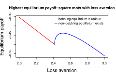
Figure 2: The babbling equilibrium is unique up to payoffs for low values of $\lambda$, but there exists an equilibrium with gradual good news for $\lambda\geq 2.414$. Due to the role of loss aversion in sustaining credible partial news, a receiver with higher loss aversion may experience higher or lower expected news utility in equilibrium than a receiver with lower loss aversion.

To illustrate, suppose $\mu(x)=\sqrt{x}$ for $x\geq 0,$ $\mu(x)=-\lambda\sqrt{-x}$ for $x<0,$ $T=2$, and $\pi_{0}=\frac{1}{2}$. Figure 2 plots the highest equilibrium payoff for different values of $\lambda.$ Receivers with higher $\lambda$ may enjoy higher equilibrium payoffs. The reason for this non-monotonicity is that for low values of $\lambda$, the babbling equilibrium is unique and increasing $\lambda$ decreases expected news utility linearly. When the new, non-babbling equilibrium emerges for large enough $\lambda$, the sender’s behavior in the new equilibrium depends on $\lambda$. Higher loss aversion carries two countervailing effects: first, a non-strategic effect of hurting welfare when $\theta=B$, as the receiver must eventually hear the bad news; second, an equilibrium effect of changing the relative amounts of good news in different periods conditional on $\theta=A$. Receivers with an intermediate amount of loss aversion enjoy higher expected news utility than receivers with low loss aversion, as the equilibrium effect leads to better “consumption smoothing” of good news across time. But, the non-strategic effect eventually dominates and receivers with high loss aversion experience worse payoffs than receivers with low loss aversion.

4.3 Deterministic Gradual Good News Equilibria

When the receiver’s loss aversion is high enough, there can exist non-babbling equilibria in the cheap-talk game. We now analyze a family of such non-babbling equilibria, where the receiver’s belief monotonically increases over time conditional on the good state. These equilibria show that the gradual good news, one-shot bad news information structures discussed in Section 3 can be sustained without commitment.

An equilibrium $(M,\sigma^{*},p^{*})$ features deterministicgradual good news (GGN equilibrium) if there exist a sequence of constants $p_{0}\leq p_{1}\leq...\leq p_{T-1}\leq p_{T}$ with $p_{0}=\pi_{0}$, $p_{T}=1$, and the receiver always has belief $p_{t}$ in period $t$ when the state is good. By Bayesian beliefs, in the bad state of any GGN equilibrium the sender must induce a belief of either $0$ or $p_{t}$ in period $t$, as any message not inducing belief $p_{t}$ is a conclusive signal of the bad state.

The class of GGN equilibria is non-empty, for it contains the babbling equilibrium where $\pi_{0}=p_{0}=p_{1}=...=p_{T-1}<p_{T}=1$. The number of intermediate beliefs in a GGN equilibrium is the number of distinct beliefs in the open interval $(\pi_{0},1)$ along the sequence $p_{0},p_{1},...,p_{T-1}$. The babbling equilibrium has zero intermediate beliefs.

The next proposition characterizes the set of all GGN equilibria with at least one intermediate belief.

Proposition 5.

Let $P^{*}(\pi)\subseteq(\pi,1]$ be those beliefs $x>\pi$ satisfying $\mu(x-\pi)+\mu(-x)=\mu(-\pi).$ Suppose $\mu$ exhibits diminishing sensitivity and loss aversion. For $1\leq J\leq T-1,$ there exists a gradual good news equilibrium with the $J$ intermediate beliefs $q^{(1)}<...<q^{(J)}$ if and only if $q^{(j)}\in P^{*}(q^{(j-1)})$ for every $j=1,...,J$, where $q^{(0)}:=\pi_{0}$.

To interpret, $P^{*}(\pi)$ contains the set of beliefs $x>\pi$ such that the sender is indifferent between inducing the two belief paths $\pi\to x\to 0$ and $\pi\to 0.$ When $\mu$ is symmetric, this indifference condition is never satisfied, which is the source of the credibility problem for good-news messages. The same indifference condition pins down the relationship between successive intermediate beliefs in GGN equilibria. This condition ensures that in the bad state, the sender is willing to randomize between revealing the state and lying with an inconclusive piece of good news that moves the receiver to the next intermediate belief.

We illustrate this result with the quadratic news utility.

Corollary 3.

1) With quadratic news utility, $P^{*}(\pi)=\left\{\pi\cdot\frac{\beta_{p}+\beta_{n}}{\beta_{p}-\beta_{n}}-\frac{\alpha_{n}-\alpha_{p}}{\beta_{p}-\beta_{n}}\right\}\cap(\pi,1).$

2a) If $\beta_{n}>\beta_{p}$, there cannot exist any gradual good news equilibrium with more than one intermediate belief.

2b) If $\beta_{n}<\beta_{p}$, there can exist gradual good news equilibria with more than one intermediate belief. For a given set of parameters of the quadratic news-utility function and prior $\pi_{0}$, there exists a uniform bound on the number of intermediate beliefs that can be sustained in equilibrium across all $T$.

3) In any GGN equilibrium with quadratic news utility, intermediate beliefs in the good state grow at an increasing rate.

For the case of quadratic news utility, this result provides a closed-form characterization of the successive intermediate beliefs. It also shows every GGN equilibrium involves progressively larger pieces of good news in the good state, $q^{(j+1)}-q^{(j)}>q^{(j)}-q^{(j-1)}$. The convex time-path of equilibrium beliefs is due to diminishing sensitivity. If the sender is indifferent between providing $d$ amount of false hope and truth-telling in the bad state when the receiver has prior belief $\pi_{L}$, then she strictly prefers providing the same amount of false hope over truth-telling at any more optimistic prior belief $\pi_{H}>\pi_{L}$. The false hope generates the same positive news utility in both cases, but an extra $d$ units of disappointment matters less when added a baseline disappointment level of $\pi_{H}$ rather than $\pi_{L}$, thanks to diminishing sensitivity.

Equilibrium beliefs in the good state grow at an increasing rate, but must be bounded above by 1. So, there exists some uniform bound $\bar{J}$ on the number of intermediate beliefs depending only on the prior belief $\pi_{0}$ and parameters of the news-utility function.

As an illustration, consider the quadratic news utility with $\alpha_{p}=2$, $\alpha_{n}=2.1$, $\beta_{p}=1$, and $\beta_{n}=0.2$. Starting at the prior belief of $\pi_{0}=\frac{1}{3}$, Figure 3 shows the longest possible sequence of intermediate beliefs in any GGN equilibrium for arbitrarily large $T$. Since the $P^{*}$ sets are either empty sets or singleton sets for the quadratic news utility, Figure 3 also contains all the possible beliefs in any state of any GGN equilibrium with these parameters.

Figure 3: The longest possible sequence of GGN intermediate beliefs starting with prior $\pi_{0}=\frac{1}{3}$. For quadratic news utility, equilibrium GGN beliefs always increase at an increasing rate in the good state.

Beyond the quadratic case, the intuition that diminishing sensitivity should cause the receiver to have a convex time-path of equilibrium beliefs holds more generally. The next result formalizes this relationship. It shows that when diminishing sensitivity is combined with a pair of regularity conditions, intermediate beliefs grow at an increasing rate in any GGN equilibrium. These conditions are satisfied, for example, by the square-roots news utility with loss aversion.

Proposition 6.

Suppose $\mu$ exhibits diminishing sensitivity, $|P^{*}(\pi)|\leq 1$ and $\frac{\partial}{\partial\epsilon}\left[\mu(\epsilon)+\mu(-(\pi+\epsilon))\right]|_{\epsilon=0}>0$ for all $\pi\in(0,1)$. Then, in any GGN equilibrium with intermediate beliefs $q^{(1)}<...<q^{(J)}$, we get $q^{(j)}-q^{(j-1)}<q^{(j+1)}-q^{(j)}$ for all $1\leq j\leq J-1$.

The first regularity condition requires that the sender is indifferent between the belief paths $\pi\to x\to 0$ and $\pi\to 0$ for at most one $x>\pi.$ It is a technical assumption that lets us prove our result, but we suspect the conclusion also holds under some relaxed conditions. The second regularity condition says in the bad state, the total news utility associated with an $\epsilon$ amount of false hope is higher than truth-telling for small $\epsilon$.

5 Related Literature and Predictions of Other Belief-Based Utility Models

5.1 Experiments on Information Preference

A number of experimental papers have tested whether people prefer one-shot resolution by asking subjects to choose how they wish to learn about their prize for the experiment, with one-shot resolution as a feasible information structure. The empirical results are mixed. After accounting for preference over the timing of resolution, Falk and Zimmermann (2023) and Bellemare, Krause, Kröger, and Zhang (2005) find evidence that subjects prefer one-shot resolution, while Nielsen (2020); Masatlioglu, Orhun, and Raymond (2017); Zimmermann (2014); Budescu and Fischer (2001) find evidence against it. News utility with diminishing sensitivity may explain these mixed results, as it predicts one-shot resolution is neither the best nor the worst information structure, so it may or may not be chosen depending on what other information structures are feasible in a particular experiment. On the other hand, these experimental results are harder to reconcile with theories that either predict agents always choose one-shot resolution or predict agents always avoid it.

Two experiments have examined people’s preference over the skewness of news, with mixed results. Tables 10 and 11 in Nielsen (2020) report that subjects prefer negatively skewed news, as predicted by news utility with diminishing sensitivity. But, Masatlioglu, Orhun, and Raymond (2017) find that agents prefer positively skewed news. In showing that a classical assumption of reference dependence leads to a prediction about preference over news skewness, we hope to stimulate further empirical work on this topic.

Finally, consistent with the mechanism discussed in Section 3, Gul, Natenzon, Ozbay, and Pesendorfer (2020) find in an experiment that more people choose gradual information over early one-shot resolution when the gradual information features gradual good news rather than gradual bad news.

5.2 Related Work on New Utility

Since Kőszegi and Rabin (2009), several other authors have analyzed the implications of news utility in different settings: asset pricing (Pagel, 2016), life-cycle consumption (Pagel, 2017), portfolio choice (Pagel, 2018), and mechanism design (Duraj, 2019). These papers focus on Bayesian agents with two-part linear gain-loss utilities and do not study the role of diminishing sensitivity to news.

Interpreting monetary gains and losses as news about future consumption, experiments that show risk-seeking behavior when choosing between loss lotteries and risk-averse behavior when choosing between gain lotteries provide evidence for diminishing sensitivity over consumption news (see e.g., Rabin and Weizsäcker (2009)). In the same vein, papers in the finance literature that use diminishing sensitivity over monetary gains and losses to explain the disposition effect (Shefrin and Statman, 1985; Kyle, Ou-Yang, and Xiong, 2006; Barberis and Xiong, 2012; Henderson, 2012) also provide indirect evidence for diminishing sensitivity over consumption news.

Bowman, Minehart, and Rabin (1999) study a consumption-based reference-dependent model with diminishing sensitivity. A critical difference is that their reference points are based on past habits, not rational expectations. We are not aware of existing work that focuses on how diminishing sensitivity matters for information design with news utility.

5.3 Predictions of Other Belief-Based Utility Models

In general, papers on belief-based utility have highlighted two sources of felicity: levels of belief about future consumption utility (“anticipatory utility,” e.g., Kőszegi (2006); Eliaz and Spiegler (2006); Schweizer and Szech (2018)) and changes in belief about future consumption utility (“news utility” and “suspense and surprise” (Ely, Frankel, and Kamenica, 2015)). For the latter, some function of both the prior belief and the posterior belief serves as the carrier of utility, while a given posterior belief brings the same anticipatory utility for all priors (Eliaz and Spiegler, 2006). The rich information preference under news utility with diminishing sensitivity contrast against more stark predictions of the other commonly used models of belief-based utility in the behavioral literature.

5.3.1 News Utility without Diminishing Sensitivity

The literature on reference-dependent preferences and news utility has focused on two-part linear gain-loss utility functions, which violate diminishing sensitivity. If $\mu$ is two-part linear with loss aversion, then it follows from the martingale property of Bayesian beliefs that one-shot resolution is weakly optimal for the agent among all information structures. If there is strict loss aversion, then one-shot resolution does strictly better than any information structure that resolves uncertainty gradually.

5.3.2 Anticipatory Utility

In our setup, an agent who experiences anticipatory utility gets $A\left(\sum_{\theta\in\Theta}\pi_{t}(\theta)\cdot v(c_{\theta})\right)$ if he ends period $t$ with posterior belief $\pi_{t}\in\Delta(\Theta),$ where $A:\mathbb{R}\to\mathbb{R}$ is a strictly increasing anticipatory-utility function. When $A$ is the identity function (as in Kőszegi (2006)), the solution to the optimization problem would be unchanged if we modified our model and let the agent experience both anticipatory utility and news utility. This is because by the martingale property, the agent’s ex-ante expected anticipatory utility in a given period is the same across all information structures. So, the ranking of information structures entirely depends on the news utility they generate.

For a general $A$, if the agent only experiences anticipatory utility, not news utility, then there exists an optimal information structure that only releases information in $t=1$, followed by uninformative signals in all subsequent periods (see Online Appendix OA 2.2). By contrast, this kind of one-shot resolution is not optimal when the agent has diminishing sensitivity and weak enough loss aversion.

5.3.3 Suspense and Surprise

Ely, Frankel, and Kamenica (2015) study dynamic information design with a Bayesian receiver who derives utility from suspense or surprise. They propose and study an original utility function over belief paths where larger belief movements always bring greater felicity. By contrast, because our states are associated with different consumption consequences, changes in beliefs may increase or decrease the receiver’s utility depending on whether the news is good or bad. While one-shot resolution is suboptimal in both Ely, Frankel, and Kamenica (2015)’s problem and our problem (under some conditions), other results differ. For example, information structures featuring gradual bad news, one-shot good news are worse than one-shot resolution in our problem, while one-shot resolution is the worst possible information structure in Ely, Frankel, and Kamenica (2015)’s problem.

Ely, Frankel, and Kamenica (2015) also discuss state-dependent versions of suspense and surprise utilities, but this extension does not embed our model. Suppose there are two states, $\Theta=\{G,B\},$ and the agent has the suspense objective $\sum_{t=0}^{T-1}u\left(\mathbb{E}_{t}(\sum_{\theta}\alpha_{\theta}\cdot(\pi_{t+1}(\theta)-\pi_{t}(\theta))^{2}\right)$ or the surprise objective $\sum_{t=1}^{T}u\left(\sum_{\theta}\alpha_{\theta}\cdot(\pi_{t}(\theta)-\pi_{t-1}(\theta))^{2}\right)$, where $\alpha_{G},\alpha_{B}>0$ are state-dependent scaling weights. We must have $\pi_{t+1}(G)-\pi_{t}(G)=-(\pi_{t+1}(B)-\pi_{t}(B))$, so pathwise $(\pi_{t+1}(G)-\pi_{t}(G))^{2}=(\pi_{t+1}(B)-\pi_{t}(B))^{2}$. This shows that the new objectives obtained by applying two possibly different scaling weights $\alpha_{G}\neq\alpha_{B}$ to states $G$ and $B$ are identical to the ones that would be obtained by applying the same scaling weight $\alpha=\frac{\alpha_{G}+\alpha_{B}}{2}$ to both states. Due to this symmetry in preference, the optimal information structure for entertaining an agent with state-dependent suspense or surprise utility treats the two states symmetrically, in contrast to a central prediction of diminishing sensitivity in our model.

5.3.4 Designing Beliefs through Non-Informational Channels

Brunnermeier and Parker (2005) and Macera (2014) study the optimal design of beliefs for agents with belief-based utilities that differ from the news-utility setup we consider. Another important distinction is that we focus on the design of information: changes in the agent’s belief derive from Bayesian updating an exogenous prior, using the information conveyed by an information structure or by a sender. Macera (2014) considers a non-Bayesian agent who freely chooses a path of beliefs, while knowing the actual state of the world. Brunnermeier and Parker (2005) study the “opposite” problem to ours, where the agent freely chooses a prior belief (over the sequence of state realizations) at the start of the game, then updates belief about future states through an exogenously given information structure.

5.4 Related Decision-Theoretic Work on Information Preference

Several paper in decision theory have studied models of preference over dynamic information structures. Dillenberger (2010) shows that preference for one-shot resolution of uncertainty is equivalent to a weakened version of independence, provided the preference satisfies recursivity. This result does not apply here because our mean-based model of news utility violates recursivity — it can be shown that a news-utility agent may strictly prefer a 0% chance of winning a prize over a 1% chance of winning it, if he will gradually learn about the outcome of the lottery and has high enough loss aversion (see Online Appendix OA 2.1). Dillenberger and Raymond (2020) axiomatize a general class of additive belief-based preferences in the domain of two-stage lotteries, relaxing recursivity and the independence axiom. In the case of $T=2,$ our news-utility model belongs to the class they characterize. Under this specialization, our work may be thought of as studying the information design problem, with and without commitment, using some of Dillenberger and Raymond (2020)’s additive belief-based preferences. Gul, Natenzon, and Pesendorfer (2021) axiomatize a class of preferences over non-instrumental information called risk consumption preferences, including a novel “peak-trough” utility specification. In contrast, we study the implications diminishing sensitivity, a classical assumption from the behavioral economics literature. Our model is not a risk consumption preference (see Online Appendix OA 2.3).

5.5 Related Work in Dynamic Information Design

In a setting without behavioral preferences, Li and Norman (2021) and Wu (2018) consider a group of senders with commitment power, sequentially sending signals to persuade a single receiver. The receiver takes an action after observing all signals. In their settings, every equilibrium in their setting can be converted into a payoff-equivalent “one-step” equilibrium where the first sender sends the joint signal implied by the old equilibrium, while all subsequent senders babble uninformatively. Dynamics matter more in our setting, as different sequences of interim beliefs cause the agent to experience different amounts of total news utility.

Lipnowski and Mathevet (2018) study a static model of information design with a psychological receiver whose welfare depends directly on posterior belief. They discuss an application to a mean-based news-utility model without diminishing sensitivity in their Appendix A, finding that either one-shot resolution or no information is optimal. We focus on the implications of diminishing sensitivity. Our work also differs in that we study a dynamic problem and examine equilibria without commitment.

6 Conclusion

In this work, we have studied how diminishingly sensitive gain-loss utilities applied to changes in beliefs affect the agent’s informational preferences. If we think that diminishing sensitivity to the magnitude of news is psychologically realistic in this domain, then the stark predictions of the ubiquitous two-part linear models may be misleading. In the presence of diminishing sensitivity, richer informational preferences emerge.

An agent’s consumption preference over the states can determine his preference between an information structure that delivers news gradually and another that results in one-shot resolution. In general, one-shot resolution is neither the best way to get information nor the worst way — skewness matters. One-shot resolution is strictly better than information structures with strictly gradual bad news, one-shot good news. But, it is strictly worse than information structures with strictly gradual good news, one-shot bad news, provided loss aversion is not too high.

For an informed sender who lacks commitment power, diminishing sensitivity leads to novel credibility problems that inhibit any meaningful communication when the receiver has no loss aversion. High enough loss aversion can restore the equilibrium credibility of good-news messages, and the receiver’s equilibrium welfare may be non-monotonic in loss aversion. We construct a family of non-babbling equilibria with gradual good news when loss aversion is high enough, finding that the sender must communicate increasingly larger pieces of good news over time in the good state.

Appendix A Proofs of the Main Results

This appendix contains the proofs of the results stated in the main text. Proofs of auxiliary results stated in the appendix appear in Online Appendix OA 1.

In the proofs, we will often use the following fact about news-utility functions with diminishing sensitivity. We omit its simple proof.

Fact 1.

Let $d_{1},d_{2}>0$ and suppose $\mu(0)=0$.

• (sub-additivity in gains) If $\mu^{{}^{\prime\prime}}(x)<0$ for all $x>0$, then $\mu(d_{1}+d_{2})<\mu(d_{1})+\mu(d_{2}).$

• (super-additivity in losses) If $\mu^{{}^{\prime\prime}}(x)>0$ for all $x<0,$ then $\mu(-d_{1}-d_{2})>\mu(-d_{1})+\mu(-d_{2})$

A.1 Proof of Proposition 1

Proof.

In the less preferred state, the agent gets $\mu(-\rho_{0})$ with one-shot resolution , but $\sum_{t=1}^{T}\mu(\rho_{t}-\rho_{t-1})$ with gradual bad news, one-shot good news. For each $t,$ $\rho_{t}-\rho_{t-1}\leq 0,$ and furthermore $\sum_{t=1}^{T}\rho_{t}-\rho_{t-1}=-\rho_{0}$ by telescoping and using the fact that $\rho_{T}=0$. Due to super-additivity in losses, we get that $\mu(-\rho_{0})\geq\sum_{t=1}^{T}\mu(\rho_{t}-\rho_{t-1})$ almost surely when the state is bad. Also, because there is strictly gradual bad news, $\mathbb{E}[\sum_{t=1}^{T}\mu(\rho_{t}-\rho_{t-1})\mid\rho_{T}=0]<\mu(-\rho_{0})$.

In the more preferred state, he gets $\mu(1-\rho_{0})$ with one-shot resolution. With gradual bad news, one-shot good news, let $\hat{T}\leq T$ be the first period where $\rho_{\hat{T}}>\rho_{\hat{T}-1}$. His news utility is $\left[\sum_{t=1}^{\hat{T}-1}\mu(\rho_{t}-\rho_{t-1})\right]+\mu(1-\rho_{\hat{T}-1})$ where each $\rho_{t}-\rho_{t-1}\leq 0$ for $1\leq t\leq\hat{T}-1$. Again by super-additivity in losses, $\sum_{t=1}^{\hat{T}-1}\mu(\rho_{t}-\rho_{t-1})\leq\mu(\rho_{\hat{T}-1}-\rho_{0})$. By sub-additivity in gains, $\mu(1-\rho_{\hat{T}-1})\leq\mu(\rho_{0}-\rho_{\hat{T}-1})+\mu(1-\rho_{0})\leq-\mu(\rho_{\hat{T}-1}-\rho_{0})+\mu(1-\rho_{0})$, where the weak inequality follows since $\lambda\geq 1.$ Putting these pieces together,

$$\left[\sum_{t=1}^{\hat{T}-1}\mu(\rho_{t}-\rho_{t-1})\right]+\mu(1-\rho_{\hat{T}-1}) \leq\mu(\rho_{\hat{T}-1}-\rho_{0})-\mu(\rho_{\hat{T}-1}-\rho_{0})+\mu(1-\rho_{0})=\mu(1-\rho_{0}).$$

Therefore, strictly gradual bad news, one-shot good news gives strictly lower utility than one-shot resolution in expectation, and almost surely weakly lower utility ex-post. ∎

A.2 Proof of Proposition 2

Proof.

In the preferred state, the agent gets $\mu(1-\rho_{0})$ with one-shot resolution, but $\sum_{t=1}^{T}\mu(\rho_{t}-\rho_{t-1})$ with gradual good news, one-shot bad news. For each $t,$ $\rho_{t}-\rho_{t-1}\geq 0,$ and furthermore $\sum_{t=1}^{T}\rho_{t}-\rho_{t-1}=1-\rho_{0}$ by telescoping and using the fact that $\rho_{T}=1$. Due to sub-additivity in gains, we get that $\sum_{t=1}^{T}\mu(\rho_{t}-\rho_{t-1})\geq\mu(1-\rho_{0})$ when the state is good. Also, because there is strictly gradual good news, $\mathbb{E}[\sum_{t=1}^{T}\mu(\rho_{t}-\rho_{t-1})\mid\rho_{T}=1]>\mu(1-\rho_{0})$.

In the less preferred state, he gets $\mu(-\rho_{0})$ with one-shot resolution. With gradual good news, one-shot bad news, let $\hat{T}\leq T$ be the first period where the $X_{\hat{T}}=0$. His news utility is $\left[\sum_{t=1}^{\hat{T}-1}\mu(\rho_{t}-\rho_{t-1})\right]+\mu(-\rho_{\hat{T}-1})$ where each $\rho_{t}-\rho_{t-1}\geq 0$ for $1\leq t\leq\hat{T}-1$. Again by sub-additivity in gains, $\sum_{t=1}^{\hat{T}-1}\mu(\rho_{t}-\rho_{t-1})\geq\mu(\rho_{\hat{T}-1}-\rho_{0})$. By super-additivity in losses, $\mu(-\rho_{\hat{T}-1})\geq\mu(-(\rho_{\hat{T}-1}-\rho_{0}))+\mu(-\rho_{0})=-\mu(\rho_{\hat{T}-1}-\rho_{0})+\mu(-\rho_{0})$, where we used the symmetry of $\mu$ around 0 in the last equality. Putting these pieces together,

$$\left[\sum_{t=1}^{\hat{T}-1}\mu(\rho_{t}-\rho_{t-1})\right]+\mu(-\rho_{\hat{T}-1}) \geq\mu(\rho_{\hat{T}-1}-\rho_{0})-\mu(\rho_{\hat{T}-1}-\rho_{0})+\mu(-\rho_{0})=\mu(-\rho_{0}).$$

Therefore, strictly gradual good news, one-shot bad news provides strictly higher utility than one-shot resolution in expectation, and almost surely weakly higher utility ex-post. ∎

A.3 Proof of Corollary 1

Proof.

This follows from Proposition 2 by continuity. ∎

A.4 Proof of Corollary 2

Proof.

When $v(c_{A})=0$ and $v(c_{B})=1$, gradual information falls in the class of strictly gradual bad news, one-shot good news. So, the first claim follows from Proposition 1. When $v(c_{A})=1$ and $v(c_{B})=0$, gradual information falls in the class of strictly gradual good news, one-shot bad news. So, the second claim follows from Corollary 1. ∎

A.5 Proof of Proposition 3

Proof.

(1) Suppose $\mu$ is two-part linear with $\mu(x)=x$ for $x\geq 0,$ $\mu(x)=\lambda x$ for $x<0,$ where $\lambda\geq 0$. Suppose $v(c_{A})=1$, $v(c_{B})=0.$ In each period, $\mathbb{E}[\mu(\pi_{t}-\pi_{t-1})]=\mathbb{E}[(\pi_{t}-\pi_{t-1})^{+}-\lambda(\pi_{t}-\pi_{t-1})^{-}]$. By the martingale property, $\mathbb{E}[(\pi_{t}-\pi_{t-1})^{+}]=\mathbb{E}[(\pi_{t}-\pi_{t-1})^{-}]$, so $\mathbb{E}[\mu(\pi_{t}-\pi_{t-1})]=\frac{1}{2}(1-\lambda)\mathbb{E}[|\pi_{t}-\pi_{t-1}|]$. This shows total expected news utility is $\mathbb{E}[\sum_{t=1}^{T}\mu(\pi_{t}-\pi_{t-1})]=\frac{1}{2}(1-\lambda)\mathbb{E}[\sum_{t=1}^{T}|\pi_{t}-\pi_{t-1}|]$. Note that $\mathbb{E}[\sum_{t=1}^{T}|\pi_{t}-\pi_{t-1}|]$ is strictly larger for gradual information than for one-shot resolution. If $\lambda>1,$ the agent strictly prefers one-shot resolution. If $0\leq\lambda<1,$ the agent strictly prefers gradual information. If $\lambda=1,$ the agent is indifferent.

Now suppose $v(c_{A})=0$, $v(c_{B})=1.$ By the same arguments, total expected news utility is $\mathbb{E}[\sum_{t=1}^{T}\mu(\rho_{t}-\rho_{t-1})]=\frac{1}{2}(1-\lambda)\mathbb{E}[\sum_{t=1}^{T}|\rho_{t}-\rho_{t-1}|]$. Note that $\mathbb{E}[\sum_{t=1}^{T}|\rho_{t}-\rho_{t-1}|]$ is strictly larger for gradual information than for one-shot resolution. So again, if $\lambda>1,$ the agent strictly prefers one-shot resolution. If $0\leq\lambda<1,$ the agent strictly prefers gradual information. If $\lambda=1,$ the agent is indifferent.

(2) If $u$ is linear, then the agent is indifferent between gradual information and one-shot resolution regardless of the sign of $v(c_{A})-v(c_{B})$. If $u$ is strictly concave, then for $1\leq t\leq T-1$, $\mathbb{E}[u(\rho_{t})]<u(\rho_{0})$ by combining the martingale property and Jensen’s inequality. So the agent strictly prefer to keep his prior beliefs until the last period and will therefore choose one-shot resolution, regardless of the sign of $v(c_{A})-v(c_{B})$.

(3) Ely, Frankel, and Kamenica (2015) mention a “state-dependent” specification of their suspense and surprise utility functions. With two states, A and B, their specification uses weights $\alpha_{A},\alpha_{B}>0$ to differentially re-scale belief-based utilities for movements in the two different directions. Specifically, their re-scaled suspense utility is

$$\sum_{t=0}^{T-1}u\left(\mathbb{E}_{t}\left[\alpha_{A}\cdot(\pi_{t+1}-\pi_{t})^{2}+\alpha_{B}\cdot((1-\pi_{t+1})-(1-\pi_{t}))^{2}\right]\right)$$

and their re-scaled surprise utility is

$$\mathbb{E}\left[\sum_{t=1}^{T}u\left(\alpha_{A}\cdot(\pi_{t+1}-\pi_{t})^{2}+\alpha_{B}\cdot((1-\pi_{t+1})-(1-\pi_{t}))^{2}\right)\right].$$

We may consider agents with opposite preferences over states A and B as agents with different pairs of scaling weights $(\alpha_{A},\alpha_{B}).$ Specifically, say there are $\alpha^{\text{High}}>\alpha^{\text{Low}}>0$. For an agent preferring A, $\alpha_{A}=\alpha^{\text{High}},\alpha_{B}=\alpha^{\text{Low}}$. For an agent preferring B, $\alpha_{A}=\alpha^{\text{Low}},\alpha_{B}=\alpha^{\text{High}}$. But note that we always have $\pi_{t+1}-\pi_{t}=-[(1-\pi_{t+1})-(1-\pi_{t})]$, so along every realized path of beliefs, $(\pi_{t+1}-\pi_{t})^{2}=((1-\pi_{t+1})-(1-\pi_{t}))^{2}$. This means these two agents with the opposite scaling weights actually have identical objectives and therefore will have the same preference over gradual information or one-shot resolution. ∎

A.6 Proof of Proposition 4

We begin by giving some additional definition and notation. For $p,\pi\in[0,1],$ let $N_{B}(x;\pi):=\mu(x-\pi)+\mu(-x)$ denote the total amount of news utility across two periods when the receiver updates his belief from $\pi$ to $x>\pi$ today and updates it from $x$ to 0 tomorrow. Similarly, $N_{A}(p;\pi):=\mu(p-\pi)+\mu(1-p)$.

We state some preliminary lemmas about $N_{A}$ and $N_{B}$, whose proofs appear in Online Appendix OA 1.

Lemma A.1.

If $\mu$ is symmetric around 0 and $\mu^{{}^{\prime\prime}}(x)<0$ for all $x>0,$ then for any $0<\pi<x<1$ it holds $N_{B}(0;\pi)<N_{B}(x;\pi)$.

Lemma A.2.

Suppose $\mu$ exhibits diminishing sensitivity and greater sensitivity to losses. Then, $p\mapsto N_{A}(p;\pi)$ is strictly increasing on $[0,\pi]$ and symmetric on the interval $[\pi,1]$. For each $p_{1}\in[\pi,1]$, there exists exactly one point $p_{2}\in[\pi,1]$ so that $N_{A}(p_{1};\pi)=N_{A}(p_{2};\pi).$ For every $p_{L}<\pi$ and $p_{H}\geq\pi,$ $N_{A}(p_{L};\pi)<N_{A}(p_{H};\pi).$ Also, $N_{B}(p;\pi)$ is symmetric on the interval $[0,\pi]$. For each $p_{1}\in[0,\pi]$, there exists exactly one point $p_{2}\in[0,\pi]$ so that $N_{B}(p_{1};\pi)=N_{B}(p_{2};\pi).$

Consider any period $T-2$ history $h_{T-2}$ in any equilibrium $(M,\sigma^{*},p^{*})$ where $p^{*}(h_{T-2})=\pi\in(0,1).$ Let $P_{A}$ and $P_{B}$ represent the sets of posterior beliefs induced at the end of $T-1$ with positive probability, in states A and B. The next lemma gives an exhaustive enumeration of all possible $P_{A},P_{B}$.

Lemma A.3.

The sets $P_{A},P_{B}$ belong to one of the following cases.

1. $P_{A}=P_{B}=\{\pi\}$

2. $P_{A}=\{1\},$ $P_{B}=\{0\}$

3. $P_{A}=\{p_{1}\}$ for some $p_{1}\in(\pi,1)$ and $P_{B}=\{0,p_{1}\}$

4. $P_{A}=\{\pi,1\}$ and $P_{B}=\{0,\pi\}$

5. $P_{A}=\{p_{1},p_{2}\}$ for some $p_{1}\in(\pi,\frac{1+\pi}{2}),$ $p_{2}=1-p_{1}+\pi$, $P_{B}=\{0,p_{1},p_{2}\}$.

We now give the proof of Proposition 4.

Proof.

Consider any period $T-2$ history $h^{T-2}$ with $p^{*}(h^{T-2})\in(0,1).$ By Lemma A.1, $N_{B}(p;p^{*}(h^{T-2}))>N_{B}(0;p^{*}(h^{T-2}))$ for all $p\in(p^{*}(h^{T-2}),1]$. Therefore, cases 3 and 5 are ruled out from the conclusion of Lemma A.3. This shows that after having reached history $h^{T-2}$, the receiver will get total news utility of $\mu(1-p^{*}(h^{T-2}))$ in the good state and $\mu(-p^{*}(h^{T-2}))$ in the bad state. This conclusion applies to all period $T-2$ histories (including those with equilibrium beliefs 0 or 1). So, the sender gets the same utility as if the state is perfectly revealed in period $T-1$ rather than $T$, and the equilibrium up to period $T-1$ form an equilibrium of the cheap talk game with horizon $T-1.$ By backwards induction, we see that along the equilibrium path, whenever the receiver’s belief updates, it is updated to the dogmatic belief in $\theta$. ∎

A.7 Proof of Proposition 5

Proof.

Let $J$ intermediate beliefs satisfying the hypotheses be given. We construct a gradual good news equilibrium where $p_{t}=q^{(t)}$ for $1\leq t\leq J$, and $p_{t}=q^{(J)}$ for $J+1\leq t\leq T-1.$

Let $M=\{a,b\}$ and consider the following strategy profile. In period $t\leq J$ where the public history so far $h^{t-1}$ does not contain any $b$, let $\sigma(h^{t-1};A)(a)=1,$ $\sigma(h^{t-1};B)(a)=x$ where $x\in(0,1)$ satisfies $\frac{p_{t-1}}{p_{t-1}+(1-p_{t-1})x}=p_{t}$. But if public history contains at least one $b,$ then $\sigma(h^{t-1};A)(b)=1$ and $\sigma(h^{t-1};B)(b)=1$. Finally, if the period is $t>J$, then $\sigma(h^{t-1};A)(b)=1$ and $\sigma(h^{t-1};B)(b)=1$. In terms of beliefs, suppose $h^{t}$ has $t\leq J$ and every message so far has been $a.$ Such histories are on-path and get assigned the Bayesian posterior belief. If $h^{t}$ has $t\leq J$ and contains at least one $b$, then it gets assigned belief 0. Finally, if $h^{t}$ has $t>J$, then $h^{t}$ gets assigned the same belief as the subhistory constructed from its first $J$ elements. It is easy to verify that these beliefs are derived from Bayes’ rule whenever possible.

We verify that the sender has no incentive to deviate. Consider period $t\leq J$ with history $h^{t-1}$ that does not contain any $b.$ The receiver’s current belief is $p_{t-1}$ by construction.

In state $B$, we first calculate the sender’s equilibrium payoff after sending $a.$ The receiver will get some $I$ periods of good news before the bad state is revealed, either by the sender or by nature in period $T.$ That is, the equilibrium news utility with $I$ periods of good news is given by $\sum_{i=1}^{I}\mu(p_{t-1+i}-p_{t-2+i})+\mu(-p_{t-1+I}).$ Since $p_{t-1+I}\in P^{*}(p_{t-2+I})$, we have $N_{B}(p_{t-1+I};p_{t-2+I})=N_{B}(0;p_{t-2+I}),$ that is to say $\mu(p_{t-1+I}-p_{t-2+I})+\mu(-p_{t-1+I})=\mu(-p_{t-2+I}).$ We may therefore rewrite the receiver’s total news utility as $\sum_{i=1}^{I-1}\mu(p_{t-1+i}-p_{t-2+i})+\mu(-p_{t-2+I})$. But by repeating this argument, we conclude that the receiver’s total news utility is just $\mu(-p_{t-1})$. Since this result holds regardless of $I$’s realization, the sender’s expected total utility from sending $g$ today is $\mu(-p_{t-1})$, which is the same as the news utility from sending $b$ today. Thus, sender is indifferent between $a$ and $b$ and has no profitable deviation.

In state $A$, the sender gets at least $\mu(1-p_{t-1})$ from following the equilibrium strategy. This is because the receiver’s total news utility in the good state along the equilibrium path is given by $\sum_{i=1}^{J-(t-1)}\mu(p_{t-1+i}-p_{t-2+i})+\mu(1-p_{t-1+I})$. By sub-additivity in gains, this sum is strictly larger than $\mu(1-p_{t-1}).$ If the sender deviates to sending $b$ today, then the receiver updates belief to 0 today and belief remains there until the exogenous revelation, when belief updates to 1. So this deviation gives the total news utility $\mu(-p_{t-1})+\mu(1)$. We have

$$\mu(1) <\mu(1-p_{t-1})+\mu(p_{t-1})$$

$$\leq\mu(1-p_{t-1})-\mu(-p_{t-1}),$$

where the first inequality comes from sub-additivity in gains, and the second from weak loss aversion. This shows $\mu(-p_{t-1})+\mu(1)<\mu(1-p_{t-1})$, so the deviation is strictly worse than sending the equilibrium message.

Finally, at a history containing at least one $b$ or a history with length $K$ or longer, the receiver’s belief is the same at all continuation histories. So the sender has no deviation incentives since no deviations affect future beliefs.

For the other direction, suppose by way of contradiction there exists a gradual good news equilibrium with the $J$ intermediate beliefs $q^{(1)}<...<q^{(J)}$. For a given $1\leq j\leq J,$ find the smallest $t$ such that $p_{t}=q^{(k-1)}$ and $p_{t+1}=q^{(k)}.$ At every on-path history $h^{t}\in H^{t}$ with $p^{*}(h^{t})=p_{t}$, we must have $\sigma^{*}(h^{t};B)$ inducing both 0 and $q^{(j)}$ with strictly positive probability. Since we are in equilibrium, we must have $\mu(-q^{(j-1)})$ being equal to $\mu(q^{(j)}-q^{(j-1)})$ plus the continuation payoff. If $j=J$, then this continuation payoff is $\mu(-q^{(j)})$ as the only other period of belief movement is in period $T$ when the receiver learns the state is bad. If $j<J,$ then find the smallest $\bar{t}$ so that $p_{\bar{t}+1}=q^{(j+1)}$. At any on-path $h^{\bar{t}}\in H^{\bar{t}}$ which is a continuation of $h^{t},$ we have $p^{*}(h^{\bar{t}})=q^{(j)}$ and the receiver has not experienced any news utility in periods $t+2,...,\bar{t}$. Also, $\sigma^{*}(h^{\bar{t}};B)$ assigns positive probability to inducing posterior belief 0, so the continuation payoff in question must be $\mu(-q^{(j)}).$ So we have shown that $\mu(-q^{(j-1)})=\mu(q^{(j)}-q^{(j-1)})+\mu(-q^{(j)}),$ that is $N_{B}(q^{(j)};q^{(j-1)})=N_{B}(0;q^{(j-1)})$. ∎

A.8 Proof of Corollary 3

Proof.

We apply Proposition 5 to the case of quadratic news utility. Recall the relevant indifference equation in the good state.

$$\mu(-q_{t})=\mu(q_{t+1}-q_{t})+\mu(-q_{t+1}).$$ (1)

Plugging in the quadratic specification and algebraic transformations lead to

$$0=(\alpha_{p}-\alpha_{n})(q_{t+1}-q_{t})-\beta_{p}(q_{t+1}-q_{t})+\beta_{n}(q_{t+1}-q_{t})(q_{t+1}+q_{t})$$

Define $r=q_{t+1}-q_{t}$. Then this relation can be written as

$$(\beta_{p}-\beta_{n})r^{2}+(\alpha_{n}-\alpha_{p}-2\beta_{n}q_{t})r=0,$$

i.e. $r$ is a zero of a second order polynomial. For $P^{*}$ to be non-empty we need this root $r$ to be in $(0,1-q_{t})$. In particular the peak/trough $\bar{r}$ of the parabola defined by the second order polynomial should satisfy $\bar{r}\in(0,\frac{1-q_{t}}{2})$. Given that $\bar{r}=\frac{2\beta_{n}q_{t}-(\alpha_{n}-\alpha_{p})}{2(\beta_{p}-\beta_{n})}$ for the case that $\beta_{p}\neq\beta_{n}$, we get the equivalent condition on the primitives $0<\frac{2\beta_{n}q_{t}-(\alpha_{n}-\alpha_{p})}{2(\beta_{p}-\beta_{n})}<\frac{1-q_{t}}{2}.$ The root $r$ itself is given by $r=\frac{2\beta_{n}q_{t}-(\alpha_{n}-\alpha_{p})}{\beta_{p}-\beta_{n}},$ which leads to the recursion

$$q_{t+1}=q_{t}\frac{\beta_{p}+\beta_{n}}{\beta_{p}-\beta_{n}}-\frac{\alpha_{n}-\alpha_{p}}{\beta_{p}-\beta_{n}}.$$ (2)

This leads to the formula for $P^{*}(\pi)$ in part 1).

Case 1: When $\beta_{p}<\beta_{n}$ the coefficient in front of $q_{t}$ is negative so that the recursion in Equation (2) leads to

$$q_{t+1}-q_{t}=q_{t}\frac{2\beta_{n}}{\beta_{p}-\beta_{n}}-\frac{\alpha_{n}-\alpha_{p}}{\beta_{p}-\beta_{n}}<0.$$

This also shows that for the case that $\beta_{p}<\beta_{n}$, a GGN equilibrium with 1 or more intermediate beliefs only exists when the prior is low enough: namely $\pi_{0}<\frac{\alpha_{n}-\alpha_{p}}{2\beta_{n}}=:q^{*}.$

Case 2: When $\beta_{p}>\beta_{n}$ the slope in Equation (2) is above $1$ so that for all priors $\pi_{0}$ large enough we get an increasing sequence $q_{t}$ which satisfies Equation (1). It is also easy to see from Equation (2) that

$$(q_{t+2}-q_{t+1})-(q_{t+1}-q_{t})=\left(\frac{\beta_{p}+\beta_{n}}{\beta_{p}-\beta_{n}}-1\right)>0,$$

proving the statement in the text after the corollary.

That an equilibrium can exist where partial good news are released for more than two periods, is shown by the example in the main text following the statement of the Corollary (see Figure 3). ∎

A.9 Proof of Proposition 6

Proof.

Since $N_{B}(p;\pi)-N_{B}(0;\pi)=0$ for $p=\pi$ and $\frac{\partial}{\partial p}N_{B}(p;\pi)|_{p=\pi}>0,$ $N_{B}(p;\pi)-N_{B}(0;\pi)$ starts off positive for $p$ slightly above $\pi.$ Given that $|P^{*}(\pi)|\leq 1,$ if we find some $p^{{}^{\prime}}>\pi$ with $N_{B}(p^{{}^{\prime}};\pi)-N_{B}(0;\pi)>0,$ then any solution to $N_{B}(p;\pi)-N_{B}(0;\pi)=0$ in $(\pi,0)$ must lie to the right of $p^{{}^{\prime}}.$

If $q^{(j)},q^{(j+1)}$ are intermediate beliefs in a GGN equilibrium, then by Proposition 5, $q^{(j)}\in P^{*}(q^{(j-1)})$ and $q^{(j+1)}\in P^{*}(q^{(j)})$. Let $p^{{}^{\prime}}=q^{(j)}+(q^{(j)}-q^{(j-1)})$. Then,

$$N_{B}(p^{{}^{\prime}};q^{(j)})-N_{B}(0;q^{(j)}) =\mu(p^{{}^{\prime}}-q^{(j)})+\mu(-p^{{}^{\prime}})-\mu(-q^{(j)})$$

$$=\mu(q^{(j)}-q^{(j-1)})+\mu(-q^{(j)}-(q^{(j)}-q^{(j-1)}))-\mu(-q^{(j)})$$

$$>\mu(q^{(j)}-q^{(j-1)})+\mu(-q^{(j-1)}-(q^{(j)}-q^{(j-1)}))-\mu(-q^{(j-1)}),$$

where the last inequality comes from diminishing sensitivity. But, the final expression is $N_{B}(q^{(j)};q^{(j-1)})-N_{B}(0;q^{(j-1)})$, which is 0 since $q^{(j)}\in P^{*}(q^{(j-1)})$. This shows we must have $q^{(j+1)}-q^{(j)}>q^{(j)}-q^{(j-1)}.$ ∎

Appendix B More Results on Preference over Information Structures

In this section, we consider an agent who commits to an information structure at time 0. We find a sufficient condition on the degrees of loss aversion and diminishing sensitivity for one-shot resolution to not be optimal across all information structures. When there are two periods, we find a sufficient condition for all optimal information structures to satisfy gradual good news, one-shot bad news. Finally, for two periods and the quadratic news-utility function, we solve for the optimal information structure in closed form.

B.1 General Notation for the Information Structure

In period 0, the agent chooses an information structure $(M,\sigma)$ to learn about the state $\theta$ over time. An information structure consists of a finite message space $M$ and a family of state-contingent message distributions $\sigma=(\sigma_{t})_{t=1}^{T-1}$, where $\sigma_{t}(\cdot\mid h^{t-1},\theta)\in\Delta(M)$ is a distribution over messages in period $t$ that depends on the history $h^{t-1}\in H^{t-1}:=(M)^{t-1}$ of messages so far, as well as the true state $\theta$.

The agent commits to how he will learn about $\theta$ once he chooses an information structure. He will mechanically receive messages in periods $1,2,...,T-1$ according to $\sigma$. At the end of period $t$ for $1\leq t\leq T-1$, the agent forms the Bayesian posterior belief $\pi_{t}$ about the state based on the history $h^{t}\in H^{t}$ of $t$ messages. We normalize $v(c_{A})=1,v(c_{B})=0$, so the agent’s news utility in period $1\leq t\leq T$ is $\mu(\pi_{t}-\pi_{t-1}).$

B.2 Sub-Optimality of One-Shot Resolution and Optimality of Gradual Good News, One-Shot Bad News

First, we give a sufficient condition on the news-utility function for one-shot resolution to be strictly suboptimal.

Proposition A.1.

For any $T$, one-shot resolution is strictly suboptimal if

$$\mu(1-\pi_{0})-\mu(-\pi_{0})+\mu^{{}^{\prime}}(0^{+})-\mu^{{}^{\prime}}(1-\pi_{0})+\mu(-1)>0.$$

We will soon explain that the condition in Proposition A.1 has the interpretation of “strong enough diminishing sensitivity relative to loss aversion.” The intuition behind the result, assuming this interpretation of its condition, is that an information structure that makes the agent either 99% certain that the state is good or fully confident that the state is bad improves on one-shot resolution. Starting with an interim belief of 0.99, the agent will receive another small piece of good news with high probability in the future, and that future news will still deliver sizable positive news utility by diminishing sensitivity. Of course, the agent will also become disappointed on rare occasions, but the relative weakness of loss aversion limits the disutility of this event. (It is easy to show that if $\mu$ is instead two-part linear, then one-shot resolution is optimal.)

Now we explain why the condition in this result can be thought of as a race between loss aversion and diminishing sensitivity. The quadratic news utility provides a clear illustration of this interpretation: the condition holds if and only if there is enough curvature relative to the size of the “kink” at 0.

Corollary A.1.

For quadratic news utility, Proposition A.1’s condition is equivalent to $\alpha_{n}-\alpha_{p}<\beta_{n}+\beta_{p}$.

On the left-hand side, $\alpha_{n}-\alpha_{p}=\mu^{{}^{\prime}}(0^{-})-\mu^{{}^{\prime}}(0^{+})$, which is the amount of loss aversion in quadratic news utility near 0. On the right-hand side, $\beta_{p}$ and $\beta_{n}$ control the amounts of curvature in the positive and negative regions, respectively, and correspond to the extent of diminishing sensitivity.

The interpretation of “strong enough diminishing sensitivity relative to loss aversion” also extends to a general $\mu.$ We have $\mu(1-\pi_{0})-\mu(-\pi_{0})>0$, so Proposition A.1’s condition is satisfied whenever $\mu^{{}^{\prime}}(0^{+})-\mu^{{}^{\prime}}(1-\pi_{0})+\mu(-1)>0$. We always have $\mu^{{}^{\prime}}(0^{+})-\mu^{{}^{\prime}}(1-\pi_{0})>0,$ and it increases when $\mu$ becomes more concave in the positive region. We have $\mu(-1)<0,$ but it increases when $\mu$ is more convex in the negative region. So diminishing sensitivity, in the gains or losses domain, increase the expression $\mu^{{}^{\prime}}(0^{+})-\mu^{{}^{\prime}}(1-\pi_{0})+\mu(-1)$. On the other hand, holding fixed $\mu^{{}^{\prime}}(0^{+})$ and the curvature $\mu^{{}^{\prime\prime}}(x)$ for $x\neq 0$, increasing the amount of loss aversion near 0 (i.e., $\mu^{{}^{\prime}}(0^{-})-\mu^{{}^{\prime}}(0^{+}))$ decreases $\mu(-1)$.

The next result presents a necessary and sufficient condition for inconclusive bad news to be suboptimal when $T=2.$ We then verify the condition for quadratic news utility. Let $U_{1}(\pi_{1}\mid\pi_{0})$ be the sum of the agent’s expected news utilities in periods 1 and 2, if he updates his belief to $\pi_{1}\in[0,1]$ at the end of period 1. So $U_{1}(\pi_{1}\mid\pi_{0})=\mu(\pi_{1}-\pi_{0})+\pi_{1}\cdot\mu(1-\pi_{1})+(1-\pi_{1})\cdot\mu(-\pi_{1})$.

Proposition A.2.

For $T=2$, information structures with $\mathbb{P}_{(M,\sigma)}[\pi_{1}<\pi_{0}\text{ and }\pi_{1}\neq 0]>0$ are strictly suboptimal if and only if there exists some $q\geq\pi_{0}$ so that the chord connecting $(0,U_{1}(0\mid\pi_{0}))$ and $(q,U_{1}(q\mid\pi_{0}))$ lies strictly above $U_{1}(p\mid\pi_{0})$ for all $p\in(0,\pi_{0}).$

Corollary A.2.

Quadratic news utility satisfies the condition of Proposition A.2.

If $\mu$ satisfies both conditions in Propositions A.1 and A.2, then any optimal information structure for the agent with $T=2$ must feature strictly gradual good news, one-shot bad news. In particular, we can combine Corollaries A.1 and A.2 to infer that this conclusion applies to quadratic news utility satisfying $\alpha_{n}-\alpha_{p}<\beta_{n}+\beta_{p}$.

B.3 Explicit Solution with Quadratic News Utility

We solve the optimal information structure in closed-form when the agent has a quadratic news-utility function. Suppose the parameters of $\mu$ satisfy $\alpha_{n}-\alpha_{p}<\beta_{n}+\beta_{p}$ in a $T=2$ environment. Furthermore, a concavification argument (Proposition A.4) shows that there exists an optimal information structure with binary messages that induces either belief 0 or belief $p_{H}>\pi_{0}$ in the only period of communication. We characterizes $p_{H}$ as the root of a cubic polynomial.

Proposition A.3.

For $T=2$ and quadratic news utility satisfying $\alpha_{n}-\alpha_{p}<\beta_{n}+\beta_{p},$ the optimal partial good news $p_{H}>\pi_{0}$ satisfies

$$\pi_{0}(\alpha_{n}-\alpha_{p})-(\beta_{p}+\beta_{n})\pi_{0}^{2}=p_{H}^{2}(\alpha_{n}-\alpha_{p}+\beta_{n}+\beta_{p})-p_{H}^{3}(2\beta_{p}+2\beta_{n}).$$

Let $c:=\frac{\alpha_{n}-\alpha_{p}}{\beta_{n}+\beta_{p}}$. We have $\frac{dp_{H}}{dc}>0.$ Also, we have $\frac{dp_{H}}{d\pi_{0}}<0$ when $\pi_{0}<\frac{1}{2}c$, and $\frac{dp_{H}}{d\pi_{0}}>0$ when $\pi_{0}>\frac{1}{2}c$.

There is a tension between loss aversion near the reference point (captured by $\alpha_{n}-\alpha_{p})$ and diminishing sensitivity (captured by $\beta_{n}+\beta_{p})$ in shaping the optimal information structure. Fixing the prior belief, the optimal amount of partial good news is increasing in loss aversion but decreasing in diminishing sensitivity. To understand these comparative statics, recall that in the bad state the agent will sometimes experience false hope as he gets interim good news. The agent chooses between getting (i) a larger piece of false hope with lower probability, or (ii) a smaller piece of false hope with higher probability. When there is more loss aversion near the reference point, belief paths that feature a small piece of good news followed by a small piece of bad news become much more costly, so (i) is preferred. When there is more diminishing sensitivity, the utility gap between the positive components of (i) and (ii) narrows, so (ii) becomes more favorable.

The optimal partial good news is non-monotonic in the prior belief when $\mu$ exhibits loss aversion — in that case, $p_{H}$ decreases with the prior when the prior is low, but increases with the prior when it is high. Figure A.1 illustrates. The intuition is that the agent faces competing incentives in maximizing his news utility conditional on the good state and the bad. Conditional on state $A,$ the optimal interim good news is $\frac{1}{2}(1+\pi_{0})$, which exploits diminishing sensitivity by splitting the good news evenly across two periods. Conditional on state $B$, the distortion from loss aversion discussed before pushes towards information structures that send a bigger piece of interim good news (with lower probability). For $\pi_{0}$ near 0, the agent’s expected welfare is essentially determined by his welfare in the bad state, so the latter incentive dominates and $p_{H}$ is far above 0.5. As $\pi_{0}$ increases, the relative weight on the good state’s welfare increases, so $p_{H}$ converges to $\frac{1}{2}(1+\pi_{0}).$ In the case of $\alpha_{n}=\alpha_{p}$, the distortion from loss aversion is absent, so we get $\frac{dp_{H}}{d\pi_{0}}>0$ for any $\pi_{0}\in(0,1)$.

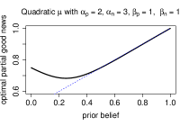
Figure A.1: Left: Optimal partial good news with $T=2$, prior $\pi_{0}=0.1,$ quadratic news utility parameters $\alpha_{p}=2,$ $\beta_{p}=1,$ $\beta_{n}=1$, as a function of $\alpha_{n}$. The optimal $p_{H}$ monotonically increases with the amount of loss aversion near 0. Right: Optimal partial good news with $T=2$, quadratic news utility parameters $\alpha_{p}=2$, $\alpha_{n}=3,$ $\beta_{p}=1,$ $\beta_{n}=1$, as a function of the prior belief. The dashed blue line shows $\pi_{0}\mapsto\frac{1}{2}(\pi_{0}+1)$, the midpoint between the prior and 1. The optimal partial good news is decreasing in the prior before $\pi_{0}=0.25$, and increasing afterwards.

B.4 Proofs of Results from Appendix B

B.4.1 Proof of Proposition A.1

Proof.

Suppose $T=2.$ Consider the following family of information structures, indexed by $\epsilon>0.$ Let $M=\{m_{L},m_{H}\}.$ Let $\sigma_{1}(A)(m_{H})=1$, and $\sigma_{1}(B)(m_{L})=x,$ $\sigma_{1}(B)(m_{H})=1-x$ for some $x\in(0,1)$ so that the posterior belief after observing $m_{H}$ is $(1-\epsilon)$.

For every $\epsilon>0,$ the difference between its expected news utility and that of one-shot resolution is $W(\epsilon),$ given by

$$\pi_{0}\cdot\left[\mu((1-\epsilon)-\pi_{0})+\mu(\epsilon)-\mu(1-\pi_{0})\right]$$

$$+ \frac{\epsilon}{1-\epsilon}\pi_{0}\cdot\left[\mu((1-\epsilon)-\pi_{0})+\mu(-(1-\epsilon))-\mu(-\pi_{0})\right].$$

$W$ is continuously differentiable away from 0 and $W(0)=0.$ To show that $W(\epsilon)>0$ for some $\epsilon>0$, it suffices that $\lim_{\epsilon\to 0^{+}}W^{{}^{\prime}}(\epsilon)>0.$ Using the continuous differentiability of $\mu$ except at 0, this limit is

$$\mu(1-\pi_{0})-\mu(-\pi_{0})+\mu^{{}^{\prime}}(0^{+})-\mu^{{}^{\prime}}(1-\pi_{0})+\mu(-1)>0.$$

If $T>2,$ then note the agent’s $T$-period problem starting with prior $\pi_{0}$ has a value at least as large as the 2-period problem with the same prior. On the other hand, one-shot resolution brings the same total expected news utility regardless of $T.$ ∎

B.4.2 Proof of Corollary A.1

Proof.

We verify Proposition A.1’s condition $\mu(1-\pi_{0})-\mu(-\pi_{0})+\mu^{{}^{\prime}}(0^{+})-\mu^{{}^{\prime}}(1-\pi_{0})+\mu(-1)>0,$ which is equivalent to $\mu^{{}^{\prime}}(0^{+})+\mu(1-\pi_{0})-\mu(-\pi_{0})>-\mu(-1)+\mu^{{}^{\prime}}(1-\pi_{0}).$ We have that

$$LHS =\alpha_{p}+\alpha_{p}(1-\pi_{0})-\beta_{p}(1-\pi_{0})^{2}-[\beta_{n}\pi_{0}^{2}-\alpha_{n}\pi_{0}]$$

$$RHS =[-\beta_{n}+\alpha_{n}]+[\alpha_{p}-2\beta_{p}(1-\pi_{0})]$$

By algebra, $LHS-RHS=(1-\pi_{0})(\alpha_{p}-\alpha_{n})+(1-\pi_{0}^{2})(\beta_{p}+\beta_{n}).$ Given that $(\alpha_{n}-\alpha_{p})\leq(\beta_{p}+\beta_{n})$ and $1-\pi_{0}^{2}>1-\pi_{0}$ for $0<\pi_{0}<1$,

$$LHS-RHS>-(1-\pi_{0}^{2})(\beta_{p}+\beta_{n})+(1-\pi_{0}^{2})(\beta_{p}+\beta_{n})=0.$$

∎

B.4.3 Backwards-Induction with Concavification

The next few results depend on an iterative concavification procedure.

For $f:\Delta(\Theta)\to\mathbb{R},$ let $\text{cav}f$ be the concavification of $f$ — that is, the smallest concave function that dominates $f$ pointwise. Concavification plays a key role in solving this information design problem, just as in Kamenica and Gentzkow (2011) and Aumann and Maschler (1995).

For $\pi_{T-2},\pi_{T-1}\in[0,1]$ two beliefs about the state, let $U_{T-1}(\pi_{T-1}\mid\pi_{T-2})$ be the sum of the agent’s expected news utilities in periods $T-1$ and $T$, if he enters period $T-1$ with belief $\pi_{T-2}$ and updates it to $\pi_{T-1}$. More precisely,

$$U_{T-1}(\pi_{T-1}\mid\pi_{T-2}):=\mu(\pi_{T-1}-\pi_{T-2})+\pi_{T-1}\cdot\mu(1-\pi_{T-1})+(1-\pi_{T-1})\cdot\mu(-\pi_{T-1}),$$

Note that by the martingale property of beliefs, if the agent holds belief $\pi_{T-1}$ at the end of period $T-1,$ then state $A$ must then realize in period $T$ with probability $\pi_{T-1}$.

Let $U_{T-1}^{*}(\pi_{T-2}):=\left(\text{cav}U_{T-1}(\cdot\mid\pi_{T-2})\right)(\pi_{T-2}).$ As we will show in the proof of Proposition A.4, $U_{T-1}^{*}(\pi_{T-2})$ is the value function of the agent if he enters period $T-1$ with belief $\pi_{T-2}.$ Continuing inductively, using the value function $U_{t+1}^{*}(\cdot)$ for $t\geq 1$, we may define $U_{t}(\pi_{t}\mid\pi_{t-1}):=\mu(\pi_{t}-\pi_{t-1})+U_{t+1}^{*}(\pi_{t}),$ which leads to the period $t$ value function $U_{t}^{*}(x):=\left(\text{cav}U_{t}(\cdot\mid x)\right)(x).$ The maximum expected news utility across all information structures is $U_{1}^{*}(\pi_{0})$, and the sequence of concavifications give the optimal information structure.

Proposition A.4.

The maximum expected news utility across all information structures is $U_{1}^{*}(\pi_{0}).$ There is an information structure $(M,\sigma)$ with $|M|=2$ attaining this maximum, with the property that after each on-path public history $h^{t-1}$ associated with belief $\pi_{t-1},$ the information structure $\sigma_{t}(\cdot\mid h^{t-1},\theta)$ induces posterior $q^{k}$ at the end of period $t$ with probability $w^{k},$ for some $q^{1},q^{2}\in[0,1],$ $w^{1},w^{2}\geq 0,$ $w^{1}+w^{2}=1$, satisfying $\sum_{k=1}^{2}w^{k}q^{k}=\pi_{t-1}$, and $U_{t}^{*}(\pi_{t-1})=\sum_{k=1}^{2}w^{k}U_{t}(q^{k}\mid\pi_{t-1})$.

The proof of Proposition A.4 appears in Online Appendix OA 1.

B.4.4 Proof of Proposition A.2

Proof.

Suppose the condition in Proposition A.2 holds. So in particular, it holds for $q=\pi_{0}.$ Consider any information structure $(M,\sigma)$ and its induced distribution over posterior beliefs in state $A$, $\eta\in\Delta([0,1]).$ If there exists $0<x<\pi_{0}$ such that $\eta(x)>0,$ then we can “split posterior $x$ into $0$ and $\pi_{0}$”: that is, we can construct another information structure $(\tilde{M},\tilde{\sigma})$ with induced distribution $\tilde{\eta}\in\Delta([0,1]),$ so that $\tilde{\eta}(x)=0,$ $\tilde{\eta}(0)=\eta(0)+\eta(x)(1-\frac{x}{\pi_{0}}),$ $\tilde{\eta}(\pi_{0})=\eta(\pi_{0})+\eta(x)\frac{x}{\pi_{0}}$. Information structure $(\tilde{M},\tilde{\sigma})$ gives strictly higher news utility than $(M,\sigma)$, since the condition implies $U_{1}(x\mid\pi_{0})<(1-\frac{x}{\pi_{0}})\cdot U_{1}(0\mid\pi_{0})+\frac{x}{\pi_{0}}\cdot U_{1}(\pi_{0}\mid\pi_{0})$.

Conversely, suppose every information structure $(M,\sigma)$ with induced posterior distribution $\eta$ such that $\eta(x)>0$ for some $0<x<\pi_{0}$ is strictly suboptimal. Then, there must exist an optimal information structure, $(\tilde{M},\tilde{\sigma})$ with posterior distribution $\tilde{\eta},$ so that $\tilde{\eta}$ is supported on two points: 0 and some $q>\pi_{0}.$ (If no information at period 1 is optimal, then one-shot resolution at period 1 is also optimal, which has $\tilde{\eta}(0)>0.$) If there exists some point $p\in(0,\pi_{0})$ that violates the condition of Proposition A.2 for this $q$, that is $U_{1}(p\mid\pi_{0})$ is at least as large as the height of the chord connecting $(0,U_{1}(0\mid\pi_{0}))$ and $(q,U_{1}(q\mid\pi_{0}))$, then an information structure inducing the posterior beliefs $p$ and $q$ would strictly dominate the optimal information structure, which is impossible. ∎

B.4.5 Proof of Corollary A.2

We first state a sufficient condition for the sub-optimality of information structures with partial bad news with $T=2$. Consider the chord connecting $(0,U_{1}(0\mid\pi_{0}))$ and $(\pi_{0},U_{1}(\pi_{0}\mid\pi_{0}))$ and let $\ell(x)$ be its height at $x\in[0,\pi_{0}]$. Let $D(x):=\ell(x)-U_{1}(x\mid\pi_{0})$.

Lemma A.4.

For this chord to lie strictly above $U_{1}(p\mid\pi_{0})$ for all $p\in(0,\pi_{0}),$ it suffices that $D^{{}^{\prime}}(0)>0,$ $D^{{}^{\prime}}(\pi_{0})<0,$ and $D^{{}^{\prime\prime}}(p)=0$ for at most one $p\in(0,\pi_{0}).$

The proof of Lemma A.4 appears in Online Appendix OA 1. Now we verify that the condition in Lemma A.4 holds for the quadratic news utility, which in turn verifies the condition of Proposition A.2 for $q=\pi_{0}$ and shows partial bad news information structures to be strictly suboptimal.

Proof.

Clearly, $D(p)$ is a third-order polynomial, so $D^{{}^{\prime\prime}}(p)$ has at most one root.

For $p<\pi_{0},$ we have the derivative

$$\frac{d}{dp}U(p\mid\pi_{0})= 2\beta_{n}(p-\pi_{0})+\alpha_{n}+\alpha_{p}(1-p)-\beta_{p}(1-p)^{2}$$

$$+p(-\alpha_{p}+2\beta_{p}(1-p))-(\beta_{n}p^{2}-\alpha_{n}p)+(1-p)(2\beta_{n}p-\alpha_{n})$$

The slope of the chord between $0$ and $\pi_{0}$ is: $\alpha_{p}-\beta_{p}+(2\beta_{p}-\alpha_{p}+\alpha_{n})\pi_{0}-(\beta_{p}+\beta_{n})\pi_{0}^{2}$. So, after straightforward algebra, $D^{{}^{\prime}}(0)=(2(\beta_{p}+\beta_{n})-(\alpha_{p}-\alpha_{n}))\pi_{0}-(\beta_{p}+\beta_{n})\pi_{0}^{2}.$ Applying weak loss aversion with $z=1$, $\alpha_{p}-\alpha_{n}\leq\beta_{p}-\beta_{n}.$ This shows

$$D^{{}^{\prime}}(0) \geq(2(\beta_{p}+\beta_{n})-(\beta_{p}-\beta_{n}))\pi_{0}-(\beta_{p}+\beta_{n})\pi_{0}^{2}$$

$$=(\beta_{p}+\beta_{n})\pi_{0}(1-\pi_{0})+2\beta_{n}\pi_{0}>0$$

for $0<\pi_{0}<1.$

We also derive $D^{{}^{\prime}}(\pi_{0})=(\alpha_{p}-2\beta_{p}-2\beta_{n}-\alpha_{n})\pi_{0}+(2\beta_{p}+2\beta_{n})\pi_{0}^{2}.$ Note that this is a convex parabola in $\pi_{0}$, with a root at 0. Also, the parabola evaluated at 1 is equal to $\alpha_{p}-\alpha_{n}\leq 0,$ where the inequality comes from the weak loss aversion with $z=0$. This implies $D^{{}^{\prime}}(\pi_{0})<0$ for $0<\pi_{0}<1.$ ∎

B.4.6 Proof of Proposition A.3

Proof.

We have

$$\frac{d}{dp}U(p\mid\pi_{0})=2\alpha_{p}-\alpha_{n}-\beta_{p}+2\beta_{p}\pi_{0}+p(-2\alpha_{p}+2\beta_{p}+2\alpha_{n}+2\beta_{n})+p^{2}(-3\beta_{p}-3\beta_{n})$$

Further, $p$ times slope of chord is:

$$U(p\mid\pi_{0})-U(0\mid\pi_{0})= U(p\mid\pi_{0})-(\beta_{n}\pi_{0}^{2}-\alpha_{n}\pi_{0})$$

$$= \pi_{0}(-\alpha_{p}+\alpha_{n})+\pi_{0}^{2}(-\beta_{p}-\beta_{n})+p(2\alpha_{p}-\alpha_{n}-\beta_{p})$$

$$+p^{2}(-\alpha_{p}+\beta_{p}+\alpha_{n}+\beta_{n})+p^{3}(-\beta_{p}-\beta_{n})+p\pi_{0}(2\beta_{p})$$

Equating $p\cdot\frac{d}{dp}U(p\mid\pi_{0})=U(p\mid\pi_{0})-U(0\mid\pi_{0})$, we get

$$\pi_{0}(\alpha_{n}-\alpha_{p})-(\beta_{p}+\beta_{n})\pi_{0}^{2}=p^{2}(\alpha_{n}-\alpha_{p}+\beta_{n}+\beta_{p})-p^{3}(2\beta_{p}+2\beta_{n}).$$

Define $c=\frac{\alpha_{n}-\alpha_{p}}{\beta_{n}+\beta_{p}}$. Note that $c\in[0,1)$ by assumptions in the statement of the Proposition.

Corollary A.2 allows us to define $p(\pi_{0},c)$ as an implicit function through $\pi_{0}c-\pi_{0}^{2}=p^{2}(1+c)-2p^{3}.$

We characterize first the derivative of $p$ w.r.t. $\pi_{0}$.

We check the conditions of the implicit function theorem in our setting: define the function $f(\pi_{0},p,c)=p^{2}(1+c)-2p^{3}-\pi_{0}c+\pi_{0}^{2}$ with domain $(0,1)^{3}$. We look at the case $c=0$ separately in the end. We need $\partial_{p}f(\pi_{0},p,c)\neq 0$. If this is true, then we can solve for $p(\pi_{0},c)$ locally and also calculate its derivative. We note that $\partial_{p}f(\pi_{0},p,c)=2p(1+c)-6p^{2}$. Hence, $\partial_{p}f(\pi_{0},p,c)$ is zero if $p=\frac{1+c}{3}=:\hat{p}\in[\frac{1}{3},\frac{2}{3}]$. Now, for a fixed $c$, we see if there is a $\pi_{0}$ that would give $\hat{p}$. This involves solving for $\pi_{0}$ in quadratic equation

$$\pi_{0}^{2}-\pi_{0}c+\frac{1}{27}(1+c)^{3}=0.$$ (3)

The discriminant as a function of $c$ is given as $D(c)=c^{2}-\frac{4}{27}(1+c)^{3}$. Note that $D^{\prime}(c)=\frac{2}{9}(2-c)(2c-1)$. In particular, $D$ is decreasing from $c=0$ to $c=\frac{1}{2}$ and increasing from then on until $c=1$. We note also that $D(0)<0,D(1)<0$ so that overall it follows that $D(c)<0$ for all $c\in[0,1]$. In particular, it holds that Equation (3) has no solution. This means that $\partial_{p}f$ never changes sign in $(0,1)^{3}\cap\{(p,\pi_{0},c):\pi_{0}c-\pi_{0}^{2}=p^{2}(1+c)-2p^{3}\}$. This also implies that $p(\pi_{0})>\frac{1+c}{3},$ for all $c,\pi_{0}\in(0,1)$. Recall here that $f$ is a smooth function on its domain. Thus, implicit function theorem is applicable for all $(\pi_{0},c)\in(0,1)^{2}$.

Totally differentiating, we get:

$$d\pi_{0}\cdot(\alpha_{n}-\alpha_{p})-(\beta_{p}+\beta_{n})2\pi_{0}\cdot d\pi_{0} =2p\cdot dp\cdot(\alpha_{n}-\alpha_{p}+\beta_{n}+\beta_{p})-3p^{2}\cdot dp\cdot(2\beta_{p}+2\beta_{n}),$$

which can be rearranged to $\frac{dp}{d\pi_{0}}\frac{1}{p}=\frac{c-2\pi_{0}}{2p^{2}(1+c)-6p^{3}}.$ The steps above showed that the denominator of this expression never changes sign. Given that we know it is negative at $c=0$ and $f$ is continuously differentiable, we conclude that the denominator is always negative for all $c$ and all $\pi_{0}\in(0,1)$. It follows that unless $c=0$, $p(\pi_{0})$ is falling until the prior characterized in the statement of the Proposition and increasing afterwards.

For the case $c=0$ one looks at the implicitly defined function $p(\pi_{0})$ through $2p^{3}(\pi_{0})-p^{2}(\pi_{0})=\pi_{0}^{2}$. Solving with similar steps as above one finds, it is strictly increasing and it is strictly above $\frac{1}{3}$ for all $\pi_{0}\in(0,1)$.

Summarizing, the amount of optimal good news can always be solved explicitly under the condition that $c\in[0,1)$ and it is always strictly above $\max\{\pi_{0},\frac{1}{3}\}$. It is strictly increasing in the prior in the absence of loss aversion and otherwise U-shaped.

Next, we focus on the derivative of $p$ w.r.t. $c$ as defined implicitly through $\pi_{0}c-\pi_{0}^{2}=p^{2}(1+c)-2p^{3}.$ We fix $\pi_{0}\in(0,1)$ and we look at the function $f:(0,1)\times(0,1)\rightarrow\mathbb{R}$ given by $f(c,p)=p^{2}(1+c)-2p^{3}-(\pi_{0}c-\pi_{0}^{2})$. The calculations above show that $f_{p}\neq 0$ for every $(c,p)\in(0,1)^{2}$. Hence, the implicit function theorem is applicable and we can calculate

$$p\frac{dp}{dc}=\frac{\pi_{0}-p^{2}}{2(1+c)-6p}.$$

Above we showed that the denominator of this expression is strictly negative. Next we show that $p(c)>\sqrt{\pi_{0}}$ for all $c\in(0,1)$. Note that the function $p\mapsto p^{2}(1+c)-2p^{3}$ is strictly decreasing in $p$ for $p>\frac{1+c}{3}$. This can be established by looking at first order derivatives. We note also that $\pi_{0}(1+c)-2\sqrt{\pi_{0}}\pi_{0}>\pi_{0}c-\pi_{0}^{2}$ is equivalent to $1-2\sqrt{\pi_{0}}+\pi=(1-\sqrt{\pi_{0}})^{2}>0$, which is true by virtue of $\pi_{0}<1$. This, and the strict monotonicity of $p\mapsto p^{2}(1+c)-2p^{3}$ for $p>\frac{1+c}{3}$ implies that $p(c)>\sqrt{\pi_{0}}$ for all $c,\pi_{0}\in(0,1)$. This establishes the result.

Summarizing, the amount of optimal good news is increasing in loss aversion as measured by $\alpha_{n}-\alpha_{p}$ and decreasing in the amount of diminishing sensitivity, as measured by $\beta_{n}+\beta_{p}$. ∎

Online Appendix

Appendix OA 1 Proof of Auxiliary Results Stated in the Appendix

OA 1.1 Proof of Lemma A.1

Proof.

Due to sub-additivity,

$$\mu(p)<\mu(p-\pi)+\mu(\pi).$$ (4)

Note that symmetry implies $\mu(-p)=-\mu(p)$ and that $\mu(-\pi)=-\mu(\pi)$. Rearranged (4) is precisely $N(0;\pi)<N(p;\pi)$. ∎

OA 1.2 Proof of Lemma A.2

Proof.

We have $\frac{\partial N_{A}(p;\pi)}{\partial p}=\mu^{{}^{\prime}}(p-\pi)-\mu^{{}^{\prime}}(1-p)$. For $0\leq p<\pi$ and under greater sensitivity to losses, $\mu^{{}^{\prime}}(p-\pi)\geq\mu^{{}^{\prime}}(\pi-p).$ Since $\mu^{{}^{\prime\prime}}(x)<0$ for $x>0,$ $\mu^{{}^{\prime}}(\pi-p)>\mu^{{}^{\prime}}(1-p)$. This shows $\frac{\partial N_{A}(p;\pi)}{\partial p}>0$ for $p\in[0,\pi).$

The symmetry results follow from simple algebra and do not require any assumptions.

Note that $\frac{\partial^{2}N_{A}(p;\pi)}{\partial p^{2}}=\mu^{{}^{\prime\prime}}(p-\pi)+\mu^{{}^{\prime\prime}}(1-p)<0$ for any $p\in[\pi,1],$ due to diminishing sensitivity. Combined with the required symmetry, this means $\frac{\partial N_{A}(p;\pi)}{\partial p}$ crosses 0 at most once on $[\pi,1],$ so for each $p_{1}\in[\pi,1]$, we can find at most one $p_{2}$ so that $N_{A}(p_{1};\pi)=N_{A}(p_{2};\pi)$. In particular, this implies at every intermediate $p_{1}\in(\pi,1),$ we get $N_{A}(p_{1};\pi)>N_{A}(\pi;\pi)$ since we already have $N_{A}(1;\pi)=N_{A}(\pi;\pi).$ This shows $N_{A}(\cdot;\pi)$ is strictly larger on $[\pi,1]$ than on $[0,\pi).$

A similar argument, using $\mu^{{}^{\prime\prime}}(x)>0$ for $x<0$, establishes that for each $p_{1}\in[0,\pi]$, we can find at most one $p_{2}$ so that $N_{B}(p_{1};\pi)=N_{B}(p_{2};\pi)$. ∎

OA 1.3 Proof of Lemma A.3

Proof.

Suppose $|P_{A}|=1.$

If $P_{A}=\{\pi\}$, then any equilibrium message not inducing $\pi$ must induce 0. By the Bayes’ rule, the sender cannot induce belief 0 with positive probability in the bad state, so $P_{B}=\{\pi\}$ as well.

If $P_{A}=\{1\},$ then any equilibrium message not inducing $1$ must induce 0. Furthermore, the sender cannot send equilibrium messages inducing belief 1 with positive probability in the bad state, else the equilibrium belief associated with these messages should be strictly less than 1. Thus $P_{B}=\{0\}$.

If $P_{A}=\{p_{1}\}$ for some $0\leq p_{1}<\pi,$ then any equilibrium message not inducing $p_{1}$ must induce 0. This is a contradiction since the posterior beliefs do not average out to $\pi.$

This leaves the case of $P_{A}=\{p_{1}\}$ for some $\pi<p_{1}<1.$ Any equilibrium message not inducing $p_{1}$ must induce 0. Furthermore, the sender must induce the belief $p_{1}$ in the bad state with positive probability, else we would have $p_{1}=1.$ At the same time, the sender must also induce belief 0 with positive probability in the bad state, else we violate Bayes’ rule. So $P_{B}=\{0,p_{1}\}$.

Now suppose $|P_{A}|=2.$

In the good state, the sender must be indifferent between two beliefs $p_{1},p_{2}$ both induced with positive probability. By Lemma A.2, $N_{A}(p;\pi)$ is strictly increasing on $[0,\pi]$ and strictly higher on $[\pi,1]$ than on $[0,\pi)$, while for each $p_{1}\in[\pi,1]$, there exists exactly one point $p_{2}\in[\pi,1]$ so that $N_{A}(p_{1};\pi)=N_{A}(p_{2};\pi).$ This means we must have $p_{1}\in[\pi,\frac{1+\pi}{2}]$, $p_{2}=1-p_{1}+\pi$.

If $P_{A}=\{\pi,1\}$, any equilibrium message not inducing $\pi$ or 1 must induce 0. Also, $1\notin P_{B},$ because any message sent with positive probability in the bad state cannot induce belief 1. We cannot have $P_{B}=\{0\}$, because then the message inducing belief $\pi$ actually induces 1. We cannot have $P_{B}=\{\pi\}$ for then we violate Bayes’ rule. This leaves only $P_{B}=\{0,\pi\}$.

If $P_{A}=\{p_{1},p_{2}\}$ for some $p_{1}\in(\pi,\frac{1+\pi}{2}),$ then any equilibrium message not inducing $p_{1}$ or $p_{2}$ must induce 0. Also, $p_{1},p_{2}\in P_{B},$ else messages inducing these beliefs give conclusive evidence of the good state. By Bayes’ rule, we must have $P_{B}=\{0,p_{1},p_{2}\}.$

It is impossible that $|P_{A}|\geq 3,$ since, by Lemma A.2, $N_{A}(p;\pi)$ is strictly increasing on $[0,\pi]$ and strictly higher on $[\pi,1]$ than on $[0,\pi)$, while for each $p_{1}\in[\pi,1]$, there exists exactly one point $p_{2}\in[\pi,1]$ so that $N_{A}(p_{1};\pi)=N_{A}(p_{2};\pi).$ So the sender cannot be indifferent between 3 or more different posterior beliefs of the receiver in the good state. ∎

OA 1.4 Proof of Proposition A.4

Proof.

We first justify by backwards induction that the value function is indeed given by $U_{t}^{*}(x)=\left(\text{cav}U_{t}(\cdot\mid x)\right)(x),$ for all $x\in[0,1]$ and all $t\leq T-1$, and that it is continuous in $x$.

If the agent enters period $t=T-1$ with the belief $x\in[0,1]$, the optimization problem over information structures is the following.

$$[Q_{T-1}]\quad\max_{\eta\in\Delta([0,1]),\mathbb{E}[\eta]=x}\int_{[0,1]}U_{T-1}(p\mid x)d\eta(p).$$

This is because any information structure $\sigma_{T-1}$ induces a Bayes plausible distribution of posterior beliefs, $\eta$ with $\mathbb{E}[\eta]=x$, and conversely every such distribution can be generated by some information structure, as in Kamenica and Gentzkow (2011). It is well-known that the value of problem $Q_{T-1}$ is $\left(\text{cav}U_{T-1}(\cdot\mid x)\right)(x)$, justifying $U_{T-1}^{*}(x)$ as the value function for any $x\in\Delta(\Theta)$. The objective in $Q_{T-1}$ is continuous in $p$ (by assumption on $\mu$) and hence in $\eta$, and furthermore the constraint set $\{\eta\in\Delta([0,1]):\mathbb{E}[\eta]=x\}$ is continuous in $x$. Therefore, $x\mapsto U_{T-1}^{*}(x)$ is continuous by Berge’s Maximum Theorem.

Assume that we have shown that value function is continuous and given by $U_{t}^{*}(x)$ for all $t\geq S$. If the agent enters period $t=S-1$ with belief $x,$ then the value of the maximization problem must be:

$$[Q_{t}]\quad\max_{\eta\in\Delta([0,1]),\mathbb{E}[\eta]=x}\int_{[0,1]}\mu(p-x)+U_{t+1}^{*}(p)d\eta(p)$$

using the inductive hypothesis that $U_{t+1}^{*}(p)$ is the period $t+1$ value function. But $\mu(p-x)+U_{t+1}^{*}(p)=U_{t}(p\mid x)$ by definition, and it is continuous by the inductive hypothesis. So by the same arguments as in the base case, $U_{S-1}^{*}(x)$ is the time-$(S-1)$ value function and it is continuous, completing the inductive step.

In the first period, by Carathéodory’s theorem, there exist weights $w^{1},w^{2}\geq 0$, beliefs $q^{1},q^{2}\in[0,1],$ with $\sum_{k=1}^{2}w^{k}=1$, $\sum_{k=1}^{2}w^{k}q^{k}=x$, such that $U_{1}^{*}(\pi_{0})=\sum_{k=1}^{2}w^{k}U_{1}(q^{k}\mid\pi_{0})$. Having now shown $U_{2}^{*}$ is the period-2 value function, there must exist an optimal information structure where $\sigma_{1}(\cdot\mid\theta)$ induces beliefs $q^{k}$ with probability $w^{k}$. This information structure induces one of the beliefs $q^{1},q^{2}$ in the second period. Repeating the same procedure for subsequent periods establishes the proposition. ∎

OA 1.5 Proof of Lemma A.4

Proof.

We need $D>0$ in the region $(0,\pi_{0})$. We know that $D(0)=D(\pi_{0})=0$. Given the conditions in the statement and the twice-differentiability of $D$ in $(0,\pi_{0})$ it follows that $D^{\prime\prime}$ changes sign only once. Moreover, it also follows that $D>0$ in a right-neighborhood of $x=0$ and a left-neighborhood of $x=\pi_{0}$. Suppose $D$ has an interior minimum at $x_{0}\in(0,\pi_{0})$. Then it holds $D^{\prime\prime}(x_{0})\geq 0$.

Suppose $D^{\prime\prime}(x)>0$ for all small $x$. Then it follows $x_{0}\leq p$, where we set $p=\pi_{0}$ if $p$ doesn’t exist. Because $D^{\prime\prime}(x)\geq 0$ for all $x\leq p$ we have that $D^{\prime}(x)>0$ for all $x\leq p$. In particular also $D(x)>0$ for all such $x$ due to the Fundamental Theorem of Calculus. Thus, the interior minimum is positive and so the claim about $D$ in $(0,\pi)$ is proven in this case.

Suppose instead that $D^{\prime\prime}(x)<0$ for all $x$ near enough to $0$. Then it follows that $x_{0}\geq p$. In particular, for all $x>p$ we have $D^{\prime\prime}(x)>0$. Since the derivative is strictly increasing for all $x\in(x_{0},\pi_{0})$ and $D^{\prime}(\pi_{0})<0$ we have that $D^{\prime}(x)<0$ for all $x\in(x_{0},\pi_{0})$. In particular, from the Fundamental Theorem of Calculus, $D(\pi_{0})$ is strictly below $D(x_{0})$. Since $D(\pi_{0})=0$ we have again that $D(x_{0})>0$.

Given the boundary values of $D$ and the signs of the derivatives at $0,\pi_{0}$ and that any interior minimum of $D$ is strictly positive, we have covered all cases and so shown that $D>0$ in $(0,\pi_{0})$. ∎

Appendix OA 2 Further Results

OA 2.1 Preference for Dominated Consumption Lotteries

So far, we have taken the prior distribution over states $\pi_{0}\in\Delta(\Theta)$ as exogenously given. Fixing an information structure, a news-utility agent may strictly prefer a dominated distribution over states. This distinguishes our news-utility preference from other preferences, such as recursive preferences and Gul, Natenzon, and Pesendorfer (2021)’s risk consumption preference.

We now give an example. Suppose $T=2$ and there are two states, $\Theta=\{A,B\}.$ Normalize consumption utility to be $v(c_{A})=1,$ $v(c_{B})=0.$ Let the news utility function be $\mu(z)=\sqrt{z}$ for $z\geq 0,$ $\mu(z)=-\lambda\sqrt{-z}$ for $z<0,$ where $\lambda\geq 1.$ At time $t=0,$ the agent holds a prior belief $\pi_{0}$ with $\pi_{0}(A)=p\in[0,1].$ At time $t=1,$ the agent learns the state perfectly, so $\pi_{1}$ is degenerate with probability 1. Consumption takes place at time $t=2.$ For any $\lambda,$ the agent strictly prefers state $A$ for sure ($\pi_{0}(A)=1$) over state $B$ for sure ($\pi_{0}(A)=0$), as both environments provide zero news utility. But, the agent may strictly prefer state $B$ for sure over an interior probability of the good state, $\pi_{0}(A)=p.$ In fact, this happens when $p+p\sqrt{1-p}-\lambda(1-p)\sqrt{p}<0$, which says $\lambda>\frac{\sqrt{p}(1+\sqrt{1-p})}{1-p}$. A sufficiently loss-averse agent may strictly prefer no chance of winning a consumption lottery than a low chance of winning.

OA 2.2 Optimal Information Structure for Anticipatory Utility

We show that if the agent has anticipatory utility and gets $A\left(\sum\pi_{t}(\theta)\cdot v(c_{\theta})\right)$ when he ends period $t$ with posterior belief $\pi_{t}\in\Delta(\Theta),$ then with commitment power, there exists an optimal information structure that only discloses information in period $t=1$.

Consider any information structure $(M,\sigma).$ Find the period $t^{*}$ with the highest ex-ante anticipatory utility, i.e., $t^{*}\in\underset{1\leq t\leq T-1}{\arg\max}\mathbb{E}_{(M,\sigma)}\left[A\left(\sum\pi_{t}(\theta)\cdot v(c_{\theta})\right)\right]$. Consider another information structure that generates the (feasible) distribution of beliefs $\pi_{t^{*}}$ in period 1, then reveals no additional information in periods $2,...,T-1.$ This new information structure gives weakly higher expected anticipatory utility than $(M,\sigma)$ in every period. Therefore there exists an optimal information structure that only discloses information in $t=1.$

OA 2.3 Risk Consumption Preferences

Gul, Natenzon, and Pesendorfer (2021) study a model of preference over random evolving lotteries and propose a class of risk consumption preferences. Translated into our setting, an agent with risk consumption preference values an information structure $(M,\sigma)$ according to utility function

$$\mathbb{E}_{(M,\sigma)}\left[\int v(u_{2}(\pi_{t}))d\eta\right].$$

Here $u_{2}:\Delta(\Theta)\to\mathbb{R}$ is affine and $v$ is strictly increasing. The term $v(u_{2}(\pi_{t}))$ is viewed as a function from the time periods $\{0,1,...,T-1\}$ into the reals and $d\eta$ denotes the Choquet integral with respect to a capacity $\eta$ on $\{0,1,...,T-1\}.$

To show that our model of mean-based news utility is not nested under the class of risk consumption preferences, we show that risk consumption preferences cannot exhibit the preference patterns from Appendix OA 2.1: that is, strictly preferring winning a lottery for sure to not winning it for sure, but also strictly preferring not winning for sure to winning with some interior probability $p\in(0,1)$ in the $T=2$ setup.

By an abuse of notation, the belief assigning probability $q$ to state $A$ will simply be denoted $q.$ The first part of the preference gives $v(u_{2}(1))>v(u_{2}(0))$, since Choquet integral of a constant function returns the same constant. When the prior winning probability is $p\in(0,1),$ the Choquet integrand is either $f_{A}:\{0,1\}\to\mathbb{R}$ with $f_{A}(0)=v(u_{2}(p))$ and $f_{A}(1)=v(u_{2}(1))$, or $f_{B}:\{0,1\}\to\mathbb{R}$ with $f_{B}(0)=v(u_{2}(p))$ and $f_{B}(0)=v(u_{2}(0))$. The two integrands correspond to belief paths where the agent wins or loses the lottery. Since $v$ is strictly increasing, $u_{2}$ is affine, and $v(u_{2}(1))>v(u_{2}(0)),$ we have $v(u_{2}(p))>v(u_{2}(0)).$ Thus both $f_{G}$ and $f_{B}$ dominate the constant function $v(u_{2}(0))$ in every period. By monotonicity of the Choquet integral, the agent must prefer $p$ probability of winning the lottery to no chance of winning it.

References

- Augenblick and Rabin (2021) Augenblick, N. and M. Rabin (2021): “Belief movement, uncertainty reduction, and rational updating,” The Quarterly Journal of Economics, 136, 933–985.
- Aumann and Maschler (1995) Aumann, R. J. and M. B. Maschler (1995): Repeated Games with Incomplete Information, Cambridge, MA: MIT Press.
- Barberis and Xiong (2012) Barberis, N. and W. Xiong (2012): “Realization utility,” Journal of Financial Economics, 104, 251–271.
- Battigalli and Dufwenberg (2022) Battigalli, P. and M. Dufwenberg (2022): “Belief-dependent motivations and psychological game theory,” Journal of Economic Literature, 60, 833–82.
- Bellemare et al. (2005) Bellemare, C., M. Krause, S. Kröger, and C. Zhang (2005): “Myopic loss aversion: Information feedback vs. investment flexibility,” Economics Letters, 87, 319–324.
- Bowman et al. (1999) Bowman, D., D. Minehart, and M. Rabin (1999): “Loss aversion in a consumption–savings model,” Journal of Economic Behavior and Organization, 38, 155–178.