Angle-Dependent Ab initio Low-Energy Hamiltonians for a Relaxed Twisted Bilayer Graphene Heterostructure

Abstract

We present efficient angle-dependent low-energy Hamiltonians to describe the properties of the twisted bilayer graphene (tBLG) heterostructure, based on ab initio calculations of mechanical relaxation and electronic structure. The angle-dependent relaxed atomic geometry is determined by continuum elasticity theory, which induces both in-plane and out-of-plane deformations in the stacked graphene layers. The electronic properties corresponding to the deformed geometry are derived from a Wannier transformation to local interactions obtained from Density Functional Theory calculations. With these ab initio tight-binding Hamiltonians of the relaxed heterostructure, the low-energy effective theories are derived from the projections near Dirac cones at K valleys. For twist angles ranging from 0.7^∘ to 4^∘, we extract both the intra-layer pseudo-gauge fields and the inter-layer coupling terms in the low-energy Hamiltonians, which extend the conventional low-energy continuum models. We further include the momentum dependent inter-layer scattering terms which give rise to the particle-hole asymmetric features of the electronic structure. Our model Hamiltonians can serve as a starting point for formulating physically meaningful, accurate interacting electron theories.

I Introduction

The physical system consisting of two layers of graphene with a small relative twist between them, referred to as twisted bilayer graphene (tBLG), has emerged as a new platform for studying correlated phases of matter since the discovery of its Mott insulator Cao et al. (2018a) and the superconducting Cao et al. (2018b) behavior. The unconventional nature of both the insulating and superconducting phases has prompted further experimental Yankowitz et al. (2019); Cao et al. (2019a); Kerelsky et al. (2018); Choi et al. (2019); Sharpe et al. (2019); Lu et al. (2019); Codecido et al. (2019) and theoretical efforts Lian et al. (2018); Wu et al. (2018a); Padhi et al. (2018); Xie and MacDonald (2018); Thomson et al. (2018); Venderbos and Fernandes (2018); González and Stauber (2019); Kennes et al. (2018); Peltonen et al. (2018); Isobe et al. (2018); Liu et al. (2018); Ochi et al. (2018); Guo et al. (2018) to better understand the physics of tBLG and related van der Waals heterostructures. Unconventional correlated phases are also observed in the heterostructures that include trilayer graphene with nearly aligned hBN substrate Chen et al. (2018, 2019) and twisted double bilayer graphene Shen et al. (2019); Liu et al. (2019); Cao et al. (2019b). The hypothesis is that a better understanding of the correlated many-body phases will emerge by exploring the many parameters available to tune the behavior of the stacked-layer hetersotstructures; these parameters include doping, external electric and magnetic fields, temperature and applied pressure Yankowitz et al. (2019). The response of the system to changes in the parameters would serve to set constraints on theoretical models, much as was the case for the isotope effect Maxwell (1950) or the effect of external magnetic fields in understanding conventional superconductivity. In contrast to the conventional three-dimensional crystalline solids, one unique adjustable parameter for tBLG and its relatives, is the twist angle between layers: by manipulating the corresponding moiré length scale through the twist angle, which can be controlled to exquisite precision, the characteristic kinetic and interaction energies can be varied without sacrificing the material quality, an effect referred to as “twistronics” Carr et al. (2017). As a consequence, the existence of the unconventional, correlated phases depends sensitively on twist angle variations Cao et al. (2018a, b); Yankowitz et al. (2019). The flat bands that emerge in the electronic spectrum at the “magic angle” ($\sim 1^{\circ}$ for tBLG) are a characteristic feature of these systems that signals the emergence of strong electron interaction effects, as first pointed out by A. McDonald and coworkers Bistritzer and MacDonald (2011a).

At the single-particle theory level, accurate theoretical modeling can capture the angle-dependent effects on the electronic structure and band topology Po et al. (2018a); Song et al. (2018); Hejazi et al. (2019), and thus serves as a starting point for formulating minimal models of interacting theories Po et al. (2018b); Koshino et al. (2018); Kang and Vafek (2018); Yuan and Fu (2018). Such theoretical modeling should take into account both the mechanical relaxation and the electronic properties. In single-layer graphene, the structural deformation can affect the electronic structure by inducing pseudo-gauge fields coupled to the Dirac electrons Mañes et al. (2013); Fang et al. (2018); Vozmediano et al. (2008, 2010). In the case of tBLG, the interaction between the two misaligned layers gives rise to a modulated structural pattern Nam and Koshino (2017); Carr et al. (2018a). The origin of the modulation is due to the varying local geometric configurations. Among these configurations, the Bernal stacking order as in the bulk graphite structure is most favorable energetically Zhou et al. (2015); Dai et al. (2016); Carr et al. (2018a). The relaxed tBLG crystal is hence determined by optimizing the stacking energy cost and elastic energy from layer deformation. Near the magic angle, the crystal relaxation can affect the electronic structure around the flat bands Nam and Koshino (2017). The single-particle gaps on both electron and hole sides of the flat bands can be accounted for by including crystal relaxation when compared with the experiments. When the twist angle is varied, the strength of atomic relaxation can be modified as well Nam and Koshino (2017); Carr et al. (2018a). It is therefore important to construct electronic models that capture these angle-dependent effects.

Given the relaxed crystal structure of a tBLG, one can model the electronic properties. A numerical scheme to model such van der Waals heterostructures has to be accurate enough to make numerical predictions that can be compared to experiment. Moreover, it should also give an intuitive physical picture that can facilitate the design of structures to enable electron correlations. The large number of atoms involved in the supercells of twisted bilayers has prevented straightforward numerical approaches. Numerical methods at different levels of sophistications from large scale density functional theory (DFT) calculations Uchida et al. (2014); Latil et al. (2007), empirical tight-binding Hamiltonians Trambly de LaissardiÚre et al. (2010); Suárez Morell et al. (2010); Trambly de Laissardière et al. (2012); Sboychakov et al. (2015); Nam and Koshino (2017) to low-energy $\bm{k}\cdot\bm{p}$ continuum theories Bistritzer and MacDonald (2011a); Lopes dos Santos et al. (2007, 2012); Mele (2011, 2010) have been employed. Among these approaches, the continuum $\bm{k}\cdot\bm{p}$ is computationally efficient and allows continuous twist angle control of the electronic band structure unconstrained by commensurate conditions Zou et al. (2018); Mele (2010); the latter type of constraints are required for DFT and tight-binding calculations. Each approach has its strengths and weaknesses in terms of numerical accuracy and efficiency.

In our work, we adopt an ab initio multi-scale numerical approach to model a tBLG which takes fully into account crystal relaxation and the twist angle dependence. Briefly, this multi-scale numerical method is designed to combine the strengths of conventional approaches mentioned above. This framework allows us to extract the relevant mechanical and electronic properties at the microscopic length scale based on ab initio total-energy and electronic structure calculations. We thus obtain a computation scheme that allows for both a clear physical picture and efficient numerical implementation, discussed in detail in the main body of the paper. Through this approach, we are able to generalize the conventional continuum $\bm{k}\cdot\bm{p}$ theory Bistritzer and MacDonald (2011a) to capture all relevant band features of ab initio methods Carr et al. (2019a). For example, one such feature is the pronounced particle-hole asymmetry in the tight-binding bands in tBLG, a theoretical prediction that remains an open question on the experiment side.

Another interesting aspect of the flat bands near the Fermi level is the topological properties of the manifold, related to the wavefunction texture in the full Brillouin Zone. In contrast with trivial atomic insulator bands which can be viewed as the Hilbert space from spatially localized orbitals, a non-trivial topological structure of the flat bands in a tBLG near the magic angle has implications on the construction of a finite $n$-band model near charge-neutrality Po et al. (2018a); Song et al. (2018). In other heterostructures, flat bands with non-trivial Chern numbers are predicted Zhang et al. (2019); Wu et al. (2019). The non-trivial topology in the manifold impacts the formation of exotic interacting phases. The accurate multi-scale modeling can provide a reliable numerical method to estimate the model parameters and investigate various perturbations and their effects on the topology of the flat bands.

The paper is structured as follows: In Sec. II, we describe the procedures in each step of the multi-scale approach, from mechanical and electronic calculations with DFT and Wannier constructions, to ab-initio tight-binding models and the derivations of effective low-energy $\bm{k}\cdot\bm{p}$ Hamiltonians based on the projection method. In Sec III, we further explore the numerical implications of our effective models which include the mechanical and electronic properties, and the scaling of coupling constants with respect to the twist angle. We conclude and summarize the discussions in Sec IV, and remark on potential applications and extensions.

II Relaxed tBLG Mechanical and Electronic Structure: A Multi-scale Approach

A van der Waals heterostructure as exemplified in a tBLG is a complicated material system to study, with massive number of atoms involved at small twist angles. For a tBLG at around the magic angle, there are about 12,000 atoms in a twisted moiré supercell. Direct simulation of a complete heterostructure requires substantial computational resources and does not yield a clear physical picture in a straightforward manner. Here we take a different approach to van der Waals heterostructure system, by a multi-scale numerical scheme as outlined in Fig. 1. This multi-scale numerical scheme is designed to combine the accuracy of DFT calculations and the transparent physical picture of efficient low-energy $\bm{k}\cdot\bm{p}$ continuum theories, connected by a simplified tight-binding Hamiltonian for a moiré supercell. Our studies begin with the mechanical and electronic modeling for the much smaller local systems sampled from the heterostructure supercell. The full physical picture of the entire heterostructure is obtained by “stitching” together this local information.

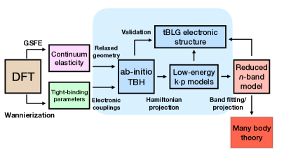
Figure 1: Schematic representation of the multi-scale numerical approach for the tBLG electronic structure, which begins at the microscopic scale where the mechanical and electronic properties of the local configuration are modeled with DFT calculations. These results are employed for the construction of ab initio tight-binding Hamiltonian and low-energy effective $\bm{k}\cdot\bm{p}$ theories. The reduced $n$-band models are further simplifications intended to form the basis for interacting many-body theories. The blocks in blue color are the focus of the present work (included in the light-blue shaded region).

The backbone of this approach, the microscopic atomic coupling and energetics, are provided by accurate DFT calculations through both the generalized stacking fault energy (GSFE), which describes the mechanical energy of the bilayer stacking Carr et al. (2018a); Zhou et al. (2015); Dai et al. (2016), and Wannier orbital coupling for the electronic properties Fang and Kaxiras (2016); Fang et al. (2018). With the GSFE, one can determine the relaxed geometry of a tBLG within continuum elasticity theory Carr et al. (2018a). The ab-initio tight-binding Hamiltonian can be constructed from the extracted Wannier couplings and applied to the relaxed geometry Fang and Kaxiras (2016). These ab-initio tight-binding Hamiltonians can be further simplified by projections onto the low-energy degrees of freedom to derive the effective $\bm{k}\cdot\bm{p}$ Hamiltonians, which are efficient ways of describing the electronic structure. Further simplifications of the $\bm{k}\cdot\bm{p}$ Hamiltonians can be carried out by projecting the lowest $n$-bands near the charge neutrality Po et al. (2018a); Carr et al. (2019a, b). Our method allows us to extract the relevant parameters based on well-defined assumptions and enables study of the twist angle dependence. In the following sections, we give more details for each step in this multi-scale numerical approach.

II.1 Mechanical Properties for Atomic Relaxation

We start by setting the conventions for a twisted bilayer graphene crystal, and describing the atomic relaxation effects. Two sheets of monolayer graphene (denoted as L1 and L2) are stacked together, with the L2 (L1) layer rotated counterclockwise (clockwise) by $\theta/2$. This small mismatch of the crystal orientations from two sheets due to this twist angle induces a long-wavelength interference pattern in the local atomic registry, alternating between locally AA, AB and BA stacking orders. We define the origin at the center of a locally AA stacking spot, which coincides with a six-fold rotational symmetry axis at the center of a hexagon in the honeycomb structure. To simplify our discussion, here we focus on the commensurate moiré supercell, which is spanned by the supercell primitive vectors $\bm{R}_{i}(i=1,2)$ and the associated supercell Brillouin zone with reciprocal lattice vectors $\bm{G}_{i}(i=1,2)$ Uchida et al. (2014). From the perspective of each individual layer, the relative twist of L1 and L2 also rotates the reciprocal lattice vectors from each layer. The differences of the reciprocal lattice vectors from each layer give rise to the supercell reciprocal lattice vectors ($\bm{G}_{i}$).

Relaxed domains of locally AB/BA stacking are energetically favored in the twisted bilayer graphene crystal Carr et al. (2018a); Zhang and Tadmor (2018). As a result of minimizing the additional energy due to the twist, the AB/BA spots are enlarged and become uniform stacking regions; these are separated by domain boundaries. Regions of AA stacking spots are reduced in size with the domain boundaries between neighboring AB/BA regions connecting the neighboring AA stacking spots. As the twist angle $\theta$ decreases, the area of AB stacking regions increases, but the domain wall width remains unchanged. This domain structure is stabilized beyond a critical twist angle Nam and Koshino (2017); Carr et al. (2018a); Zhang and Tadmor (2018). Another feature is the puckered out-of-plane crystal relaxations Uchida et al. (2014). The vertical layer separation is shortest for the AB/BA stacking regions and largest for the AA regions.

To obtain the mechanical relaxation pattern of a twisted bilayer graphene, we adopted a continuum model in combination with the GSFE Carr et al. (2018a); Zhou et al. (2015); Dai et al. (2016). To describe the structural deformation, at an unrelaxed position $\bm{r}$ in a supercell, we define the corresponding in-plane component of the displacement vector $\bm{U}^{(i)}(\bm{r})$ $(i=1,2)$ and the out-of-plane component $\bm{h}^{(i)}(\bm{r})=h^{(i)}(\bm{r})\hat{z}$ after relaxation with layer index $i$. The undeformed position $\bm{r}$ before relaxation is then mapped as $\bm{r}\rightarrow\bm{r}+\bm{U}^{(i)}(\bm{r})+h^{(i)}(\bm{r})\hat{z}$. The total mechanical energy of the twisted system has two components, the intra- and inter-layer components. The intra-layer strain energy of a single layer sheet is described by a linear isotropic continuum approximation Nam and Koshino (2017):

$$E^{\mathrm{intra}}(\bm{U}^{(i)})=\sum_{i}\int\frac{G}{2}(\partial_{x}U^{(i)}_{x}+\partial_{y}U^{(i)}_{y})^{2}$$

$$+\frac{K}{2}\left\{(\partial_{x}U^{(i)}_{x}-\partial_{y}U^{(i)}_{y})^{2}+(\partial_{x}U^{(i)}_{y}+\partial_{y}U^{(i)}_{x})^{2}\right\}d^{2}\bm{r},$$ (1)

where $G$ and $K$ are shear and bulk modulus of a monolayer graphene, which we take to be $G=9.0\,\mathrm{eV/}$Ų, $K=13.2\,\mathrm{eV/}$Ų. These values are obtained with DFT by isotropically straining and compressing the monolayer and performing a quadratic fitting of the ground-state energy as a function of the applied strain or shear.

The inter-layer energy is described by the GSFE Carr et al. (2018a); Zhou et al. (2015); Dai et al. (2016), denoted as $V_{\mathrm{GSFE}}$, which has been employed to explain relaxation in van der Waals heterostructures Carr et al. (2018a); Dai et al. (2016), and depends only on the relative stacking between two adjacent layers. We obtain the $V_{\mathrm{GSFE}}$ by applying a $9\times 9$ grid sampling of rigid shifts to L1 in the unit cell with respect to L2 and extract the relaxed ground state energy at each shift. The optimal inter-layer separation $h(\bm{r})=|h^{(1)}(\bm{r})-h^{(2)}(\bm{r})|$ is also extracted for each shifted configuration. The GSFE at any position $\bm{r}$ can then be expressed as a Fourier sum:

$$V^{\mathrm{GSFE}}(\bm{r})=\sum_{\bm{p}_{i}}V_{\bm{p}_{i}}\mathrm{e}^{i\bm{p}_{i}\cdot\bm{r}},$$ (2)

where $\bm{p}_{i}$ is defined as $\bm{p}_{i}=n_{1}\bm{G}_{1}+n_{2}\bm{G}_{2}$ for $n_{1},n_{2}$ integers, and $V_{\bm{p}_{i}}$ is the corresponding Fourier coefficient found by fitting the ground state energy at each shift. In terms of the $V^{\mathrm{GSFE}}$, the inter-layer energy $E_{\mathrm{inter}}$ can be then written as follows for a relaxed twisted bilayer:

$$E^{\mathrm{inter}}(\bm{U}^{(i)})=\int V^{\mathrm{GSFE}}(\bm{b}(\bm{r})+\bm{U}^{(1)}(\bm{r})-\bm{U}^{(2)}(\bm{r}))\,d^{2}\bm{r},$$ (3)

where $\bm{b}(\bm{r})$ is the local stacking order at an atomic position $\bm{r}$, which we can take to be the distance from the given atomic position $\bm{r}$ to the position of the nearest neighbor of the same sublattice type amd Mitchell Luskin and Massatt (2018). Note that the $V^{\mathrm{GSFE}}$ is a function of the sum of the local stacking order and the displacement vectors to describe the inter-layer stacking energy after relaxation.

The total energy is the sum of the inter-layer and the intra-layer energies:

$$E^{\mathrm{tot}}(\bm{U}^{(i)})=E^{\mathrm{intra}}(\bm{U}^{(i)})+E^{\mathrm{inter}}(\bm{U}^{(i)}),$$ (4)

where $\bm{U}^{(1)}(\bm{r})=-\bm{U}^{(2)}(\bm{r})$ due to the mirror symmetry between L1 and L2 Nam and Koshino (2017) (i.e. a $C_{2}$ rotation in three-dimensional space with an in-plane rotation axis). We then minimize the total energy as a function of the in-plane displacement field $\bm{U}^{(i)}(\bm{r})$ to obtain the optimal relaxation pattern. The relaxation pattern respects the three-fold rotation symmetry and mirror symmetry of the twisted bilayer, and the functional form can be Fourier expanded:

$$\bm{U}^{(i)}(\bm{r})=-i\sum_{\bm{p}_{i}}U_{\bm{p}_{i}}^{(i)}e^{i\bm{p}_{i}\cdot\bm{r}},h^{(i)}(\bm{r})=h^{(i)}_{0}+\sum_{\bm{p}_{i}}h^{(i)}_{\bm{p}_{i}}e^{i\bm{p}_{i}\cdot\bm{r}},$$ (5)

where symmetry requires $U^{(i)}_{\mathcal{R}_{6}\bm{p}}=\mathcal{R}_{6}U^{(i)}_{\bm{p}}$ and $h^{(i)}_{\mathcal{R}_{6}\bm{p}}=h^{(i)}_{\bm{p}}$ with $\mathcal{R}_{6}$ the $2\pi/6$ rotation matrix.

II.2 Ab-initio Tight-Binding Hamiltonian

Given a relaxed tBLG crystal with a commensurate supercell structure, the conventional Bloch theorem applies due to the presence of supercell translation symmetries. Modeling such a crystal with full DFT simulations at small twist angles is computationally demanding so we instead employ the ab initio tight-binding Hamiltonian method Fang and Kaxiras (2016); Fang et al. (2018). In this model, atomic orbital couplings are short-ranged and determined by local geometry such as the atomic registry Fang and Kaxiras (2016), layer separation Carr et al. (2018b), strain Fang et al. (2018) and orientation in the heterostructure. Calculations of the much smaller aligned bilayer structure in DFT allow us to extract the relevant tight-binding parameters and their dependence on the local geometry Fang and Kaxiras (2016); Carr et al. (2018b). This is based on the Wannier transformation of DFT calculations. The large twisted supercell structure can then be parametrized by these ab initio tight-binding Hamiltonians. We have validated the method with the full DFT simulation of a tBLG at larger twist angles Fang and Kaxiras (2016). This approach has been applied to the rigid twisted bilayers and the tBLG under external pressure Carr et al. (2018b). The scaling with pressure is consistent with the recent experiment of the tBLG in a pressure cell Yankowitz et al. (2019). The resulting accurate ab initio tight-binding Hamiltonians are still rather complicated but can be expanded to derive the simpler low-energy effective theories in the next section.

II.3 Low-Energy Effective k.p Hamiltonians

To obtain insights on the electronic structure and simpler efficient computational models, we derive the continuum low-energy effective model based on the expansion of the ab-initio tight-binding Hamiltonians of a relaxed tBLG. We begin with a brief review of the symmetries of the crystal, the low-energy effective Hamiltonian for the unrelaxed twisted bilayer graphene Bistritzer and MacDonald (2011a), and then the generalization to a relaxed crystal. This is followed by a numerical projection method to derive the effective models from ab initio tight-binding Hamiltonians, which is described in the following sections.

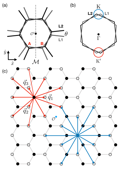
Figure 2: Conventions for a tBLG crystal and the symmetries. (a) In the real space, the twisted bilayer is generated by the rotation around the common hexagon center from an AA-stacking bilayer unit. The symmetries are defined with respect to this hexagon centers. $\mathcal{M}$ is a valley-preserving mirror symmetry which is a $180^{\circ}$ rotation with respect to an in-plane axis shown as dotted line. (b) The monolayer Brillouin zones from both layers, which are rotated from each other. The effective long-wavelength theories are expanded at either the K or K’ valleys. (c) Illustration of the low-energy $\bm{k}\cdot\bm{p}$ effective model in momentum space: the filled (empty) circles are momentum states from L1 (L2). The inter-layer (intra-layer) couplings terms with momentum $\bm{q}_{i}$ ($\bm{p}_{i}$) are represented by the red (blue) lines which connect the coupled momentum states.

Monolayer graphene features relativistic Dirac electrons at K, K’ valleys in the Brillouin zone corners. The twist angle introduces a relative displacement of Dirac cones, which originates from the same valley of each individual layer. These two copies of the Dirac electrons are then coupled through the inter-layer interaction, which is spatially varying with the moiré pattern. The scattering between Dirac electrons from the opposite valleys (K and K’) is negligible due to the much larger scattering momentum required compared to the characteristic momentum scale of the moiré pattern at small twist angle. Therefore, Dirac electrons from K and K’ valleys are essentially decoupled in the single particle description. Such valley protection and degeneracy, or the emergent valley $U_{v}(1)$ symmetry Zou et al. (2018), allows for the construction of effective models involving only one single K valley type with the opposite valley related by time reversal. Each copy of the effective model involves low-energy states enclosed in one circle in Fig. 2 (b) with the rotated monolayer Brillouin zones.

The above view of the effective $\bm{k}\cdot\bm{p}$ low-energy theory stresses its role as the expansion of the full model. On the other hand, symmetry considerations have been used as the guiding principle in constructing these low-energy models. The relevant symmetry operations for a tBLG effective $\bm{k}\cdot\bm{p}$ model include the lattice translations, $C_{3}$ rotations, valley-preserving $\mathcal{M}$ mirror symmetry and anti-unitary $C_{2}\mathcal{T}$ symmetry Zou et al. (2018). In our convention, the origin (rotation center) is chosen to be the hexagon center of a locally AA-stacking spot with the symmetries shown in Fig. 2 (a). Under these symmetries, the wavefunction $\Psi(\bm{r})=[\Psi_{\rm 1A}(\bm{r}),\Psi_{\rm 1B}(\bm{r}),\Psi_{\rm 2A}(\bm{r}),\Psi_{\rm 2B}(\bm{r})]$ transforms as

$$C_{3}: \mathcal{M}: C_{2}\mathcal{T}:$$

$$\begin{bmatrix}\bar{\phi}\Psi_{\rm 1A}(\mathcal{R}_{3}\bm{r})\\ \phi\Psi_{\rm 1B}(\mathcal{R}_{3}\bm{r})\\ \bar{\phi}\Psi_{\rm 2A}(\mathcal{R}_{3}\bm{r})\\ \phi\Psi_{\rm 2B}(\mathcal{R}_{3}\bm{r})\end{bmatrix}, \begin{bmatrix}\Psi_{\rm 2B}(\mathcal{M}\bm{r})\\ \Psi_{\rm 2A}(\mathcal{M}\bm{r})\\ \Psi_{\rm 1B}(\mathcal{M}\bm{r})\\ \Psi_{\rm 1A}(\mathcal{M}\bm{r})\end{bmatrix}, \begin{bmatrix}\Psi^{*}_{\rm 1B}(-\bm{r})\\ \Psi^{*}_{\rm 1A}(-\bm{r})\\ \Psi^{*}_{\rm 2B}(-\bm{r})\\ \Psi^{*}_{\rm 2A}(-\bm{r}),\end{bmatrix}$$ (6)

where $\phi=e^{i2\pi/3}$ ($\bar{\phi}=e^{-i2\pi/3}$), $\mathcal{R}_{3}$ rotates the vector $\bm{r}$ clockwise by $2\pi/3$ and $\mathcal{M}$ flips the $x$ coordinate of the vector $\bm{r}$ as in Fig. 2 (a). The crystal relaxation retains these relevant symmetries.

Such an effective low-energy theory expanded around the K valley has already been derived for the unrelaxed case of tBLG Bistritzer and MacDonald (2011a); Lopes dos Santos et al. (2007, 2012); Mele (2011). Since here we want to eventually include the electronic effects of relaxation, we augment this model to include additional terms that can capture these effects. With the gauge convention chosen such that the origin coincides with a locally AA-stacking spot, the augmented low-energy Hamiltonian takes the form:

$$\tilde{H}_{\rm K}=\begin{bmatrix}H^{(1)}_{D}(\bm{k})+A^{(1)}(\bm{r})&\tilde{T}^{\dagger}(\bm{r})\\ \tilde{T}(\bm{r})&H^{(2)}_{D}(\bm{k})+A^{(2)}(\bm{r}),\end{bmatrix}$$ (7)

where $H^{(i)}_{D}(\bm{k})$ is the Dirac Hamiltonian for each individual layer ($i=1,2$), and $\tilde{T}(\bm{r})$ the inter-layer coupling matrix, which varies with the spatial moiré pattern. The Dirac Hamiltonian is given by:

$$H_{D}(\bm{k})=v_{F}\begin{bmatrix}0&-ik_{+}\\ ik_{-}&0\end{bmatrix},$$ (8)

with additional Pauli matrix rotation terms to account for the small twist angle.

In the unrelaxed case, the terms $A^{(i)}(\bm{r}),i=1,2$ are set to zero, and the inter-layer coupling $\tilde{T}(\bm{r})$ is simplified to:

$$T_{\alpha\beta}(\bm{r})=\omega_{0}\begin{bmatrix}T_{0}(\bm{r})&T_{+}(\bm{r})\\ T_{-}(\bm{r})&T_{0}(\bm{r})\end{bmatrix},$$ (9)

where $T_{\alpha\beta}(\bm{r})$ specifies the coupling between various momentum states from the sublattice $\beta$ of L1 to sublattice $\alpha$ of L2, $\alpha,\beta={\rm A},{\rm B}$. In the above equations, the various symbols that appear have the following meaning: $k_{\pm}=k_{x}\pm ik_{y}$, $T_{0}(\bm{r})=e^{i\bm{q}_{1}\cdot\bm{r}}+e^{i\bm{q}_{2}\cdot\bm{r}}+e^{i\bm{q}_{3}\cdot\bm{r}}$, $T_{-}(\bm{r})=e^{i\bm{q}_{1}\cdot\bm{r}}+\phi e^{i\bm{q}_{2}\cdot\bm{r}}+\bar{\phi}e^{i\bm{q}_{3}\cdot\bm{r}}$, $T_{+}(\bm{r})=e^{i\bm{q}_{1}\cdot\bm{r}}+\bar{\phi}e^{i\bm{q}_{2}\cdot\bm{r}}+\phi e^{i\bm{q}_{3}\cdot\bm{r}}$. $\bm{q}_{1}=k_{D}\hat{x}$, $\bm{q}_{2}=k_{D}(-\hat{x}-\sqrt{3}\hat{y})/2$ and $\bm{q}_{3}=k_{D}(-\hat{x}+\sqrt{3}\hat{y})/2$ with $k_{D}=(8\pi/3a_{G})\sin(\theta/2)$ and $a_{G}$ being the graphene lattice constant, as shown in Fig. 2 (c). The inter-layer coupling strength is $\omega_{0}\approx$ 110 meV. The moiré supercell has reciprocal lattice vectors $\bm{G}_{1}=\bm{q}_{1}-\bm{q}_{2}$ and $\bm{G}_{2}=\bm{q}_{3}-\bm{q}_{2}$. The Hamiltonian can be shown to preserve the symmetries above. One interesting observation is that the coupling $T(\bm{r})$ is not periodic under moiré supercell translations Bistritzer and MacDonald (2011b) due to the field expansion gauge choice around the Dirac point of each individual layer. The two shifted Dirac cones are connected by $\bm{q}_{1}$ as in Fig. 2 (b) and (c). We will re-examine this labeling of momentum states which would facilitate the projection from the full tight-binding Hamiltonian.

To determine the set of coupled momentum states, we first look for the momentum states in each layer that are folded onto the same supercell momentum label. With $\bm{k}_{i}$ being the momentum measured from the ${\rm K}^{(i)}$ valley, this requires ${\rm K}^{(1)}+\bm{k}_{1}={\rm K}^{(2)}+\bm{k}_{2}+\bm{G}$, where $\bm{G}$ is a reciprocal lattice vector of the moiré supercell spanned by $\bm{G}_{i}$. The set of $\bm{k}_{i}$ momentum states of each layer (filled and empty circles) that are folded to the supercell $\Gamma$ point are shown in Fig. 2 (c), which is a bipartite lattice in momentum space. In the absence of the deformation from lattice relaxation, the exact translation symmetry within each single layer eliminates the direct intra-layer coupling terms between momentum states. This leaves only the inter-layer coupling $T(\bm{r})$ to be determined. The inter-layer coupling $T(\bm{r})$ describes the coupling between states at momentum $\bm{k}_{2}-\bm{k}_{1}=({\rm K}^{(1)}-{\rm K}^{(2)})-\bm{G}$, which does not belong to moiré supercell reciprocal lattice vectors. In a rigid tBLG, the dominant contributions in $T(\bm{r})$ can be derived from the orbital coupling in the microscopic tight-binding Hamiltonian Bistritzer and MacDonald (2011a). The low-energy Hamiltonian can be viewed as a momentum lattice with only nearest neighbor couplings. The $2\times 2$ coupling matrices to the three nearest neighbors direction $\bm{q}_{i}$ are:

$$T_{1}=\omega_{0}\begin{bmatrix}1&1\\ 1&1\end{bmatrix},\;\;T_{2}=\omega_{0}\begin{bmatrix}1&\bar{\phi}\\ \phi&1\end{bmatrix},\;\;T_{3}=\omega_{0}\begin{bmatrix}1&\phi\\ \bar{\phi}&1\end{bmatrix}.$$ (10)

A momentum cutoff is also imposed for the momentum lattice within the linear Dirac cone regime.

To generalize the above effective Hamiltonian for a twisted bilayer crystal with atomic relaxation within the plane (in-plane strain) as well as height variations (out-of-plane strain), we start with a deformed monolayer graphene with a strain field $\bm{U}^{(i)}(\bm{r})$, which describes the displacement vector of the underlying constituent atoms, moving the atom to a new position $\bm{r}\rightarrow\bm{r}+\bm{U}^{(i)}(\bm{r})+h^{(i)}(\bm{r})\hat{z}$ on the $i$-th layer. The in-plane strain is known to appear in the low-energy theory as the pseudo-gauge field with $A^{(i)}(\bm{r})$ a $2\times 2$ matrix which couples with the Dirac Hamiltonian $H_{D}^{(i)}(\bm{k})+A^{(i)}(\bm{r})$ Mañes et al. (2013). The isotropic part of the strain $(\partial_{x}U^{(i)}_{x}+\partial_{y}U^{(i)}_{y})$ or the deformation potential contributes to the diagonal part of $A^{(i)}(\bm{r})$, while the off-diagonal elements are given by the coupling to $(\partial_{x}U^{(i)}_{x}-\partial_{y}U^{(i)}_{y})$ and $(\partial_{x}U^{(i)}_{y}+\partial_{y}U^{(i)}_{x})$ strain components dictated by symmetry. The spatially varying $A^{(i)}(\bm{r})$ matrix introduced by the atomic deformation induces coupling between different momentum states within the same single layer. The $A^{(i)}(\bm{r})$ matrix can be decomposed into Fourier components at moiré supercell reciprocal lattice vectors. Strain perturbations are also known to renormalize the local Fermi velocity of the Dirac electron and give anisotropic velocity corrections Mañes et al. (2013). Here, we only retain the contributions in the form of the $A^{(i)}(\bm{r})$ matrix, which causes scatterings between the momentum states. For a twisted bilayer, the mirror symmetry will relate the $A^{(i)}(\bm{r})$ between the two layers.

Regarding the inter-layer coupling, the deformation field $\bm{U}^{(i)}(\bm{r})+h^{(i)}(\bm{r})\hat{z}$ from relaxation causes additional relative shifts in the local atomic registry, which modifies the $T(\bm{r})$ coupling matrix. The height variations in the moiré supercell weaken the inter-layer coupling in the locally AA stacking region (due to its larger vertical separation) and enhance the coupling in the enlarged AB/BA domains. This causes the off-diagonal coupling constants in $\tilde{T}(\bm{r})$ to be larger than the diagonal components. The dominant $T_{1}$ above with atomic relaxation becomes $\omega_{0}\sigma_{0}+\omega_{1}\sigma_{x}$ with $\omega_{0}<\omega_{1}$. These corrections are relevant for the single-particle gaps above and below the flat bands near the magic angle. Furthermore, the domain line formation and the finer structure from the atomic relaxation enhances the scattering with higher momentum components. The dependence of the coupling parameters on the twist angle will be discussed later.

In short summary, the intra-layer deformation of each of the two layers introduces the non-zero scattering terms, $A^{(i)}(\bm{r})$, in Eq. (7). The Dirac electrons from the two layers are then coupled through the inter-layer $\tilde{T}(\bm{r})$ term, which is also modified by the atomic relaxation. Later, we will include another correction term to the inter-layer coupling that involves momentum dependence of the scattered momentum states.

The effects of various coupling terms here can also be visualized from the momentum space representation of the Hamiltonian. For simplicity, we first focus on the supercell $\Gamma$ point in momentum space. The relevant momentum states from both layers are represented by the circles in Fig. 2 (c). The inter-layer coupling from $\tilde{T}(\bm{r})$ links the states from both layers, while the intra-layer $A^{(i)}(\bm{r})$ connects states reside within the same layer. We can expand these coupling terms into the Fourier momentum components

$$A^{(i)}(\bm{r})=\sum_{\bm{p}_{i}}A^{(i)}_{\bm{p}_{i}}e^{i\bm{p}_{i}\cdot\bm{r}},\;\;\tilde{T}(\bm{r})=\sum_{\bm{q}_{i}}\tilde{T}_{\bm{q}_{i}}e^{i\bm{q}_{i}\cdot\bm{r}},$$ (11)

with the twelve $\bm{q}_{i}$ ($\bm{p}_{i}$) momentum vectors illustrated in Fig. 2 (c). The $\bm{p}_{i}$ vectors are the reciprocal lattice vectors of the moiré supercell, $\bm{p}_{i}=n_{1}\bm{G}_{1}+n_{2}\bm{G}_{2}$ and the general $\bm{q}_{i}$ vectors are $({\rm K}^{(1)}-{\rm K}^{(2)})-\bm{G}^{{}^{\prime}}$. These correction terms introduce further neighbor couplings in the momentum lattice to the model as in Fig. 2 (c).

We now discuss how the symmetries in the low-energy theory constrain the forms of the coupling terms. For the $C_{3}$ and $C_{2}\mathcal{T}$ symmetries, which do not flip the layer indices, we let $F(\bm{r})$ represent either of $A^{(i)}(\bm{r})$ or $\tilde{T}(\bm{r})$ $2\times 2$ matrices. These symmetries dictate

$$C_{3} : e^{i(2\pi/3)\sigma_{z}}F(\mathcal{R}_{3}^{-1}\bm{r})e^{-i(2\pi/3)\sigma_{z}}=F(\bm{r}),$$ (12)

$$C_{2}\mathcal{T} : \sigma_{x}F^{*}(-\bm{r})\sigma_{x}=F(\bm{r}),$$ (13)

($\mathcal{R}_{3}^{-1}$ rotates $\bm{r}$ counterclockwise) with the Pauli matrices $\bm{\sigma}=(\sigma_{x},\sigma_{y},\sigma_{z})$ acting on the sublattice degree of freedom. As for the $\mathcal{M}$ mirror symmetry that flips the layer, we can derive the following relations

$$\mathcal{M} : \sigma_{x}\tilde{T}(\mathcal{M}\bm{r})\sigma_{x}=\tilde{T}^{\dagger}(\bm{r}),\;\;\sigma_{x}A^{(1)}(\mathcal{M}\bm{r})\sigma_{x}=A^{(2)}(\bm{r}),$$ (14)

and similarly for $A^{(1)}\leftrightarrow A^{(2)}$ in the last equation. When these $2\times 2$ matrices are decomposed into Fourier momentum components, these symmetry conditions yield the following equivalent constraints on the expanded matrix components:

$$C_{3} : e^{i\frac{2\pi}{3}\sigma_{z}}F_{\mathcal{R}_{3}^{-1}\bm{g}_{i}}e^{-i\frac{2\pi}{3}\sigma_{z}}=F_{\bm{g}_{i}},$$ (15)

$$C_{2}\mathcal{T} : \sigma_{x}F^{*}_{\bm{g}_{i}}\sigma_{x}=F_{\bm{g}_{i}},$$ (16)

$$\mathcal{M} : \sigma_{x}A^{(1)}_{\mathcal{M}\bm{p}_{i}}\sigma_{x}=A^{(2)}_{\bm{p}_{i}},\;\sigma_{x}\tilde{T}_{-\mathcal{M}\bm{q}_{i}}\sigma_{x}=\tilde{T}_{\bm{q}_{i}}^{\dagger}.$$ (17)

In the original effective model Bistritzer and MacDonald (2011a), only the first three $\bm{q}_{i}$’s (connections to the nearest neighbors) from $\tilde{T}_{\bm{q}_{i}}$ are included. Even though these three $\bm{q}_{i}$’s are shown to be the dominant contribution in an unrelaxed twisted bilayer, relaxation would not only modify the matrix elements but also enhance the higher momentum components.

II.4 Low-Energy Expansion based on Ab-initio Tight-Binding Hamiltonian

Here, we summarize the procedure to extract these relevant matrix elements for both the pseudo-gauge field $A^{(i)}(\bm{r})$ and inter-layer coupling $\tilde{T}(\bm{r})$ in the effective low-energy theory, derived from an ab initio tight-binding Hamiltonian of relaxed twisted bilayer graphene.

(i) For a relaxed commensurate twisted bilayer with atomic relaxation, the supercell is spanned by the translation vectors $\bm{R}_{i}$. Two integers $M$ and $N$ are used to specify the twist angle Uchida et al. (2014). The origin is chosen to be at the center of the hexagon as in Fig. 2 (a). We adopt the series $M=N+1$ commensurate supercells which have vanishing twist angles with increasing $M$ and exactly one AA-stacking region in a supercell unit. For an unrelaxed twisted bilayer, these specify all the atomic positions $\bm{r}_{l}$ in a supercell. The relaxation moves an atom to a new position by $\bm{r}_{l}\rightarrow\bm{r}_{l}+\bm{U}^{(i)}(\bm{r}_{l})+h^{(i)}(\bm{r}_{l})\hat{z}$ and modifies the coupling strength between atomic pairs. Given a supercell momentum $\bm{k}_{\rm SC}$, we define the Bloch wave as

$$|\Psi_{l}(\bm{k}_{\rm SC})\rangle=\frac{1}{\sqrt{N_{\rm SC}}}\sum_{\bm{R}}e^{i\bm{k}_{\rm SC}\cdot(\bm{r}_{l}+\bm{R})}|\bm{r}_{l}+\bm{R}\rangle,$$ (18)

where $N_{\rm SC}$ is the total number of supercells. Note that the original unrelaxed position $\bm{r}_{l}+\bm{R}$ is used in the definition even though the actual relaxed position is $\bm{r}_{l}+\bm{U}^{(i)}(\bm{r}_{l})+h^{(i)}(\bm{r}_{l})\hat{z}+\bm{R}$. The Hamiltonian $H^{\rm TBH}(\bm{k}_{\rm SC})$ in the supercell reciprocal space can be derived as:

$$H^{\rm TBH}_{lm}(\bm{k}_{\rm SC})=\sum_{\bm{R},\bm{R}^{\prime}}t_{\bm{r}_{l}+\bm{U}^{(i)}(\bm{r}_{l})+\bm{R},\bm{r}_{m}+\bm{U}^{(j)}(\bm{r}_{m})+\bm{R}^{\prime}}$$ (19)

$$\times e^{-i\bm{k}_{\rm SC}\cdot(\bm{r}_{l}+\bm{R}-\bm{r}_{m}-\bm{R}^{\prime})}.$$

(ii) The relevant states at low-energy are the Bloch waves near the K valley of both layers.

$$|\Phi_{\alpha}({\rm K}^{(i)}+\bm{k}^{(i)})\rangle$$

$$=\frac{1}{\sqrt{N_{\rm SC}N_{\alpha}}}\sum_{\bm{R}}\sum_{\bm{r}_{l}\in\alpha}e^{i({\rm K}^{(i)}+\bm{k}^{(i)})\cdot(\bm{r}_{l}+\bm{R})}|\bm{r}_{l}+\bm{R}\rangle$$

$$=\frac{1}{\sqrt{N_{\alpha}}}\sum_{\bm{r}_{l}\in\alpha}e^{i\bm{G}^{\prime}\cdot\bm{r}_{l}}|\Psi_{l}(\bm{k}_{\rm SC})\rangle,$$ (20)

with $i=1,2$ being the layer index, $\alpha=A,B$ the sublattice index, and $\bm{k}^{(i)}$ is the momentum measured relative to ${\rm K}^{(i)}$. These states are defined with the unrelaxed original positions and momentum labeling from graphene primitive unit cell translations. To be compatible with the translational symmetry of the above Hamiltonian $H^{\rm TBH}(\bm{k}_{\rm SC})$, the momentum states must be such that they can be folded to the supercell $\bm{k}_{\rm SC}$ point in momentum space. This yields the condition ${\rm K}^{(i)}+\bm{k}^{(i)}=\bm{G}^{\prime}+\bm{k}_{\rm SC}$ with $\bm{G}^{\prime}$ being a supercell reciprocal lattice vector. Given a supercell momentum $\bm{k}_{\rm SC}$, we can then construct a set of Bloch plane wave states for both layers to sample the low-energy sector of the Hamiltonian. The unrelaxed $\bm{r}_{l}+\bm{R}$ positions of atoms used in the Bloch phase factors ensure the orthogonality of the projection basis states, for a crystal with or without atomic relaxation. The state $|\Phi_{\alpha}({\rm K}^{(i)}+\bm{k}^{(i)})\rangle$ in the tight-binding orbital picture is mapped to the plane wave state on $i$-th layer with momentum $\bm{k}^{(i)}$ in the low-energy $\bm{k}\cdot\bm{p}$ expansion. We will use this picture to bridge the tight-binding and low-energy $\bm{k}\cdot\bm{p}$ pictures.

(iii) Having established the tight-binding Hamiltonian and the relevant low-energy states $|\Phi_{\alpha}({\rm K}^{(i)}+\bm{k}^{(i)})\rangle$, we can project out the coupling matrix elements in $A_{\bm{p}_{j}}^{(i)}$ and $\tilde{T}_{\bm{q}_{j}}$ for the low-energy Hamiltonian. For example, the intra-layer scattering terms from $A^{(i)}_{\alpha\beta}$ with momentum $\bm{p}_{j}$ can be inferred from $\langle\Phi_{\alpha}({\rm K}^{(i)}+\bm{k}^{(i)}+\bm{p}_{j})|H^{\rm TBH}(\bm{k}_{\rm SC})|\Phi_{\beta}({\rm K}^{(i)}+\bm{k}^{(i)})\rangle$ with ${\rm K}^{(i)}+\bm{k}$ and ${\rm K}^{(i)}+\bm{k}+\bm{p}_{j}$ both folded to $\bm{k}_{\rm SC}$. The inter-layer coupling $\tilde{T}_{\alpha\beta}$ at momentum $\bm{q}_{j}$ can be obtained from $\langle\Phi_{\alpha}({\rm K}^{(2)}+\bm{k}+\bm{q}_{j})|H^{\rm TBH}({\bm{k}_{\rm SC})}|\Phi_{\beta}({\rm K}^{(1)}+\bm{k})\rangle$ with the momentum transfer $\bm{q}_{j}$ and compatible momentum states. Numerically, the coupling matrix is obtained from the average of sampling $\bm{k}_{\rm SC}$ and $\bm{k}^{(i)}$ momenta near the K valley that are scattered into new states. The reconstructed low-energy $\bm{k}\cdot\bm{p}$ Hamiltonian captures most essential features of the tight-binding electronic band structure as shown in Fig. 3 (c). To further improve the particle-hole asymmetry of the bands, we identify the relevant terms to be added to the low-energy theory in the next section.

Figure 3: (a) A comparison of the band structures from decoupled bilayers, one without relaxation (thick green lines) and one with relaxation (purple lines). The in-plane and out-of-plane relaxation can open band gaps at high-symmetry points. (b-d) Band structures benchmarked for effective $\bm{k}\cdot\bm{p}$ bilayer Hamiltonians at $\theta=1.05^{\circ}$ with a momentum lattice cutoff radius of $6|\bm{G}|$. The full tight-binding reference bands are in thick grey lines and the $\bm{k}\cdot\bm{p}$ bands are in red. We show examples for both the unrelaxed bandstructure (b) and the relaxed bandstructure, (c) without momentum-dependent and (d) with momentum-dependent $\tilde{T}^{\prime}(\bm{r},\hat{k}_{\pm})$ terms in Eq. (21).

II.5 Momentum-Dependent Inter-layer Coupling

Experimentally, it is interesting to investigate whether the tBLG is particle-hole symmetric or not under electrical gating and the implications for the correlated insulating and superconducting phases. For the electronic structures, higher order terms in the Dirac Hamiltonian, Pauli matrix rotations, due to the twist angle Song et al. (2018) and electric potential from doping Guinea and Walet (2018) are known to give rise to particle-hole asymmetric bands. In our model, we have included the Pauli matrix rotations but they are not adequate to fully capture the asymmetric bands in the tight-binding calculations as shows in Fig. 3 (c). The projection method introduced above from the full tight-binding Hamiltonian enables us to systematically extract and identify various terms and approximations. In the above $\bm{k}\cdot\bm{p}$ low-energy Hamiltonian, the inter-layer couplings between $|\Phi_{\alpha}^{(2)}({\rm K}^{(2)}+\bm{k}+\bm{q}_{j})\rangle$ and $|\Phi_{\beta}^{(1)}({\rm K}^{(1)}+\bm{k})\rangle$ states are assumed to only depend on the momentum transfer $\bm{q}_{j}$. However, there is no protecting symmetry for this property and the coupling constants could generally depend on the momentum $\bm{k}$ as well. This dependence is explicitly seen in our numerical projection method. To elucidate these momentum-dependent correction terms, we focus here on the first three dominant $\bm{q}_{j}$ contributions, which gives the following form

$$\begin{split}\tilde{T}^{\prime}(\bm{r},\hat{k}_{\pm})=&\frac{i}{2}\begin{bmatrix}\lambda_{1}\big{\{}T_{-}(\bm{r}),\hat{k}_{+}\big{\}}&\lambda_{3}\big{\{}T_{0}(\bm{r}),\hat{k}_{+}\big{\}}\\ \lambda_{2}\big{\{}T_{+}(\bm{r}),\hat{k}_{+}\big{\}}&\lambda_{1}\big{\{}T_{-}(\bm{r}),\hat{k}_{+}\big{\}}\end{bmatrix}\\ &-\frac{i}{2}\begin{bmatrix}\lambda_{1}\big{\{}T_{+}(\bm{r}),\hat{k}_{-}\big{\}}&\lambda_{2}\big{\{}T_{-}(\bm{r}),\hat{k}_{-}\big{\}}\\ \lambda_{3}\big{\{}T_{0}(\bm{r}),\hat{k}_{-}\big{\}}&\lambda_{1}\big{\{}T_{+}(\bm{r}),\hat{k}_{-}\big{\}}\end{bmatrix},\end{split}$$ (21)

where $\lambda_{2}\approx 2\lambda_{1}\approx 0.18$ eV$\cdot$Å, $\lambda_{3}\approx 0$ around $\theta=1^{\circ}$ and the anti-commutator form for non-commuting operators. We have added this leading momentum-dependent scattering terms in the inter-layer coupling, $\tilde{T}(\bm{r})+\tilde{T}^{\prime}(\bm{r},\hat{k}_{\pm})$, and they indeed can capture the particle-hole asymmetry as shown in Fig. 3 (d). The projected low-energy bands are in good agreement with the full ab initio tight-binding electronic structure.

III Numerical Results For Angular Dependence

The effective models presented above are derived for twist angles in the range of $0.7^{\circ}$ to $4^{\circ}$. A series of commensurate $(M,N)$ supercells with $M=N+1$ are used to extract the model parameters in this range. For the general twist angles, the parameters can be obtained by interpolating the results of the commensurate cases. The numerical results are presented in their Fourier component version. There are two sets of crystal momenta involved in the expansions. The first is denoted as $\bm{p}_{i}=n_{1}\bm{G}_{1}+n_{2}\bm{G}_{2}$ which can be expressed by the moiré supercell reciprocal lattice vectors $\bm{G}_{i}$. The other second can be written as $\bm{q}_{i}$ as in Fig. 2. The differences between $\bm{q}_{i}$ vectors are reciprocal lattice vectors of the moiré supercell. Hence, any $\bm{q}_{i}$ can be written as $\bm{q}_{i}=\bm{q}_{1}+m_{1}^{i}\bm{G}_{1}+m_{2}^{i}\bm{G}_{2}$. The $\bm{q}_{i}$ are the basis for the inter-layer coupling expansion, while the $\bm{p}_{i}$ are for the intra-layer expansion (strain). Terms evaluated from momenta of identical magnitude tend to only differ by a complex phase dictated by symmetries. For this reason, we organize the $\bm{p}$ and $\bm{q}$ dependent terms by “shells” of equidistant momenta. For example, in Fig. 2, there are three shells of $\bm{q}$ (in red) and two shells of $\bm{p}$ (in blue). In summarizing the strength of terms in the expansion, it is more convenient to compare the average magnitudes of different shells instead of the complex values of individual momenta, so we label these terms as $T_{s_{j}}$ and $A_{s_{j}}$ instead of $T_{\bm{q}_{i}}$ and $A^{(i)}_{\bm{p}_{i}}$

We begin with the mechanical properties of the relaxed twisted bilayer graphene. The competition between the stacking energy and the strain energy will depend on the twist angle which determines the moiré length scale. The atomic structure will tend to reduce to the area of the unfavorable $AA$ stacking, while increasing the area of the favorable Bernal stacking ($AB$ and $BA$). The displacement field in Eq. (5) can be expanded into the Fourier components at momenta $\bm{p}_{i}$. A real-space image of the atomic relaxation is provided in Fig. 4, along with the angle-dependent magnitudes of the representative $\bm{p}_{i}$ from the first three shells.

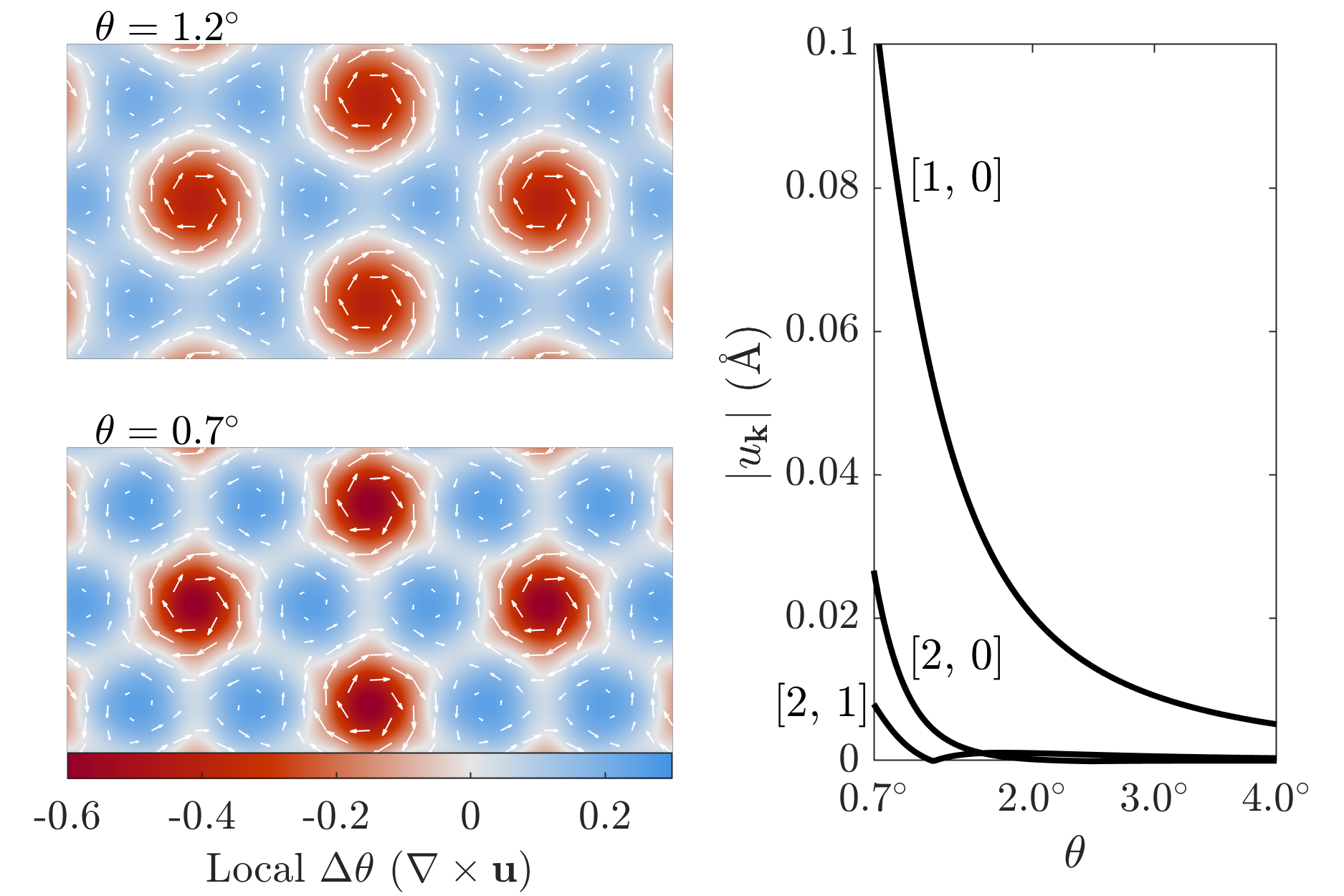
Figure 4: (Left) Relaxation patterns of L2 for bilayers with twist angles $\theta=1.2^{\circ}$ and $0.7^{\circ}$ from the continuum model. The local relaxation is given by the white arrows, and the curl of the relaxation (local change in twisting angle) is given by color. (Right) Twist-angle dependence of the relaxation coefficients $u_{\bm{p}_{i}}$, where the label $[n_{1},n_{2}]$ corresponds to $\bm{p}_{i}=n_{1}\bm{G}_{1}+n_{2}\bm{G}_{2}$.

The atomic deformation induces a pseudo-gauge field coupled to the Dirac electrons in each layer. The pseudo-gauge can also be Fourier expanded at $\bm{p}_{i}$ momenta, and then easily included in the $\bm{k}\cdot\bm{p}$ Hamiltonian. The crystal relaxation also modifies the inter-layer coupling. Both the $\tilde{T}(\bm{r})$ and the momentum-dependent corrections $\tilde{T}^{\prime}(\bm{r})$ are affected. The diagonal inter-layer coupling term (labeled $\tilde{T}^{(AA)}$) is generally smaller than the off-diagonal coupling (labeled $\tilde{T}^{(AB)}$), as the $AA$ stacking has a larger inter-layer distance (and thus smaller electronic coupling) than the $AB$ and $BA$ regions. The $AA$ coupling is further reduced at small angles by the reduction of the overall $AA$ stacking area, while the $AB$ coupling is increased. The dependence of all electronic terms on twist angle for the relaxed tBLG system is given in Fig. 5.

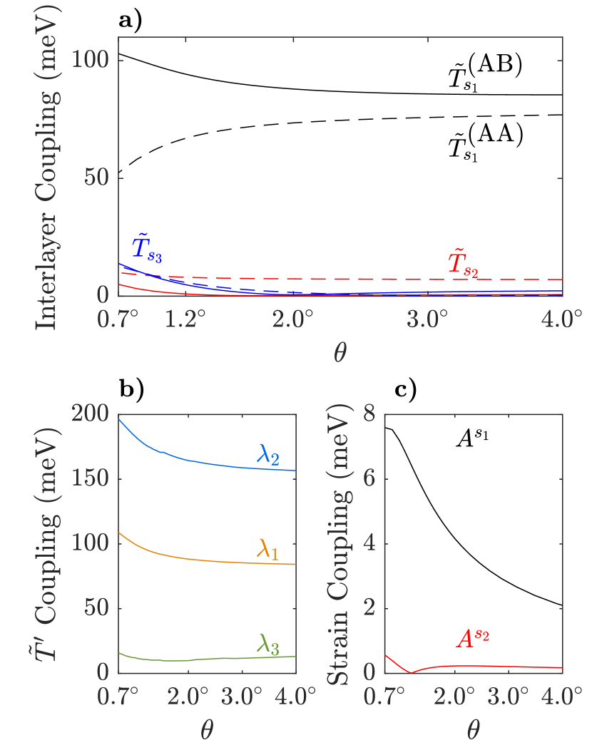
Figure 5: Twist-angle dependence of various parameters in the $\bm{k}\cdot\bm{p}$ model. (a) Magnitudes of inter-layer coupling terms $\tilde{T}_{i}$ for the three nearest shells ($s_{j}$) of couplings (red lines in Fig. 2 (c).). The off-diagonal elements of the $\tilde{T}$ matrices (AB) are shown by solid lines, while the diagonal elements (AA) by dashed lines. (b) The three $\lambda_{i}$ momentum-dependent parameters. (c) Magnitudes of the intra-layer coupling terms, ${A}^{(i)}$ for the two nearest shells ($s_{j}$) of couplings (blue lines in Fig. 2(c).).

Using the fitted $\bm{k}\cdot\bm{p}$ parameters, band structures can be calculated for tBLG systems at an arbitrary twist angle (Fig. 6). These band structures are essentially identical to those of the full tight-binding model (see Fig. 3d). Our model predicts an inversion of the two low-energy bands at $0.98^{\circ}$, but has nearly flat bands in a range of angles from $0.95^{\circ}$ to $1.05^{\circ}$. For further analysis and discussion of the low-energy electronic structure and its angle-dependence we defer to a companion work, Ref. Carr et al., 2019a.

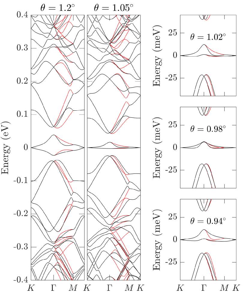
Figure 6: Twist-angle dependence of the low energy band structure of relaxed tBLG, calculated using the relaxed $k\cdot p$ model. The black lines are for an expansion around the monolayer K valley, while the red lines are for the monolayer K’ valley. At $\theta=0.98^{\circ}$, the upper and lower flat bands at the $\Gamma$ point pass smoothly through one another due to opposite mirror symmetry eigenvalues Carr et al. (2019a).

IV CONCLUSION

In this work, we adopted a systematic multi-scale approach to the modeling of tBLG with an angle dependence and relaxation effects included. Starting with DFT calculations, the mechanical and electronic properties are extracted to model the relaxed geometry through ab-initio tight-binding Hamiltonians. We then simplify the models by low-energy $\bm{k}\cdot\bm{p}$ expansions to capture the essential electronic features of the derived ab initio tight-binding Hamiltonians Carr et al. (2019a). Our approach provides an unified and coherent method to derive and simplify the modeling process while preserving the important physics, which paves the way for formulating interacting-electron theories (The model scripts are available at https://github.com/stcarr/kp_tblg).

There are also other factors that may affect the electronic structure of tBLG that are not included in our current modeling. Such factors are the hBN substrate effects on tBLG crystal relaxation and electronic couplings, screening effects from the substrate used Qiu et al. (2017), electrical gating, and self-consistent electric potential from the electron doping Guinea and Walet (2018). Disorder and additional strain variations Bi et al. (2019) across the samples introduced by the fabrication process might also complicate the interpretation of the observed behavior Kerelsky et al. (2018). Our multi-scale method provides a framework for generalizing the models to include corrections or to estimate the energy scale for such perturbations.

Our multi-scale numerical framework can be easily extended to other van der Waals heterostructures such as a few-layer graphene stacks Lee et al. (2019); Zhang et al. (2019), and transition metal dichalcogenides stacks Wu et al. (2019, 2018b). The effect of mechanical relaxation can also be included in modeling the band structure of twisted trilayer graphene stacks Zhu et al. (2019). Following the scheme of Fig. 1, one can derive models at various levels of approximation and scaling of the parameters in conjunction with the relevant symmetry analysis. Further experimental probes to the electronic and mechanical properties can also be used to refine the numerical models. This will close the design loop in predicting the properties of van der Waals heterostructures, towards establishing these systems as a new platform for exploring the physics of correlated electrons.

Appendix A Density Functional Theory Calculations

The DFT calculations in this work were carried out using the Vienna Ab initio Simulation Package (VASP) Kresse and Furthmüller (1996); Kresse and FurthmÃŒller (1996) with Projector Augmented-Wave (PAW) type of pseudo-potentials, parametrized by Perdew, Burke and Ernzerhof (PBE) Perdew et al. (1996). A slab geometry with a 20 Å vacuum region is used to reduce the interactions between periodic images. The DFT calculations are converged with plane-wave energy cutoff $500$ eV and a reciprocal space Monkhorst-Pack grid sampling of size $17\times 17\times 1$.

For the mechanical relaxation, the Generalized Stacking Fault Energy (GSFE) was calculated by performing rigid shift of the unit cell and calculate the ground state energy from DFT, and we used a $9\times 9$ grid in a unit cell for the computation. We fix the in-plane positions and allow the out-of-plane positions to relax. We implemented the van der Waals force through the vdW-DFT method using the SCAN+rVV10 functional Klimeš et al. (2011); Peng et al. (2016).

The extended Bloch wavefunction basis can be transformed into the maximally-localized Wannier functions (MLWF) basis as implemented in the Wannier90 code Mostofi et al. (2008). With this transformation, the effective tight-binding Hamiltonian for a designated group of bands of the material can be constructed. This not only gives an efficient numerical method to reproduce DFT results but also provides a physically transparent picture of localized atomic orbitals and their hybridizations. Our work is based on the systematic analysis of such tight-binding Hamiltonians, which inherit the ab initio information without fitting procedures for the numerical parameters Fang and Kaxiras (2016). Further corrections for band gaps from advanced GW calculations or other choices of exchange correlation functionals are also compatible with Wannier constructions.

References

- Cao et al. (2018a) Y. Cao, V. Fatemi, A. Demir, S. Fang, S. L. Tomarken, J. Y. Luo, J. D. Sanchez-Yamagishi, K. Watanabe, T. Taniguchi, E. Kaxiras, R. C. Ashoori, and P. Jarillo-Herrero, Nature 556, 80 EP (2018a).
- Cao et al. (2018b) Y. Cao, V. Fatemi, S. Fang, K. Watanabe, T. Taniguchi, E. Kaxiras, and P. Jarillo-Herrero, Nature 556, 43 EP (2018b).
- Yankowitz et al. (2019) M. Yankowitz, S. Chen, H. Polshyn, Y. Zhang, K. Watanabe, T. Taniguchi, D. Graf, A. F. Young, and C. R. Dean, Science (2019), 10.1126/science.aav1910, http://science.sciencemag.org/content/early/2019/01/25/science.aav1910.full.pdf .
- Cao et al. (2019a) Y. Cao, D. Chowdhury, D. Rodan-Legrain, O. Rubies-Bigordà, K. Watanabe, T. Taniguchi, T. Senthil, and P. Jarillo-Herrero, “Strange metal in magic-angle graphene with near planckian dissipation,” (2019a), arXiv:1901.03710 .
- Kerelsky et al. (2018) A. Kerelsky, L. McGilly, D. M. Kennes, L. Xian, M. Yankowitz, S. Chen, K. Watanabe, T. Taniguchi, J. Hone, C. Dean, A. Rubio, and A. N. Pasupathy, “Magic angle spectroscopy,” (2018), arXiv:1812.08776 .
- Choi et al. (2019) Y. Choi, J. Kemmer, Y. Peng, A. Thomson, H. Arora, R. Polski, Y. Zhang, H. Ren, J. Alicea, G. Refael, F. von Oppen, K. Watanabe, T. Taniguchi, and S. Nadj-Perge, “Imaging electronic correlations in twisted bilayer graphene near the magic angle,” (2019), arXiv:1901.02997 .
- Sharpe et al. (2019) A. L. Sharpe, E. J. Fox, A. W. Barnard, J. Finney, K. Watanabe, T. Taniguchi, M. A. Kastner, and D. Goldhaber-Gordon, “Emergent ferromagnetism near three-quarters filling in twisted bilayer graphene,” (2019), arXiv:1901.03520 .
- Lu et al. (2019) X. Lu, P. Stepanov, W. Yang, M. Xie, M. A. Aamir, I. Das, C. Urgell, K. Watanabe, T. Taniguchi, G. Zhang, A. Bachtold, A. H. MacDonald, and D. K. Efetov, “Superconductors, orbital magnets, and correlated states in magic angle bilayer graphene,” (2019), arXiv:1903.06513 .
- Codecido et al. (2019) E. Codecido, Q. Wang, R. Koester, S. Che, H. Tian, R. Lv, S. Tran, K. Watanabe, T. Taniguchi, F. Zhang, M. Bockrath, and C. N. Lau, “Correlated insulating and superconducting states in twisted bilayer graphene below the magic angle,” (2019), arXiv:1902.05151 .
- Lian et al. (2018) B. Lian, Z. Wang, and B. A. Bernevig, “Twisted bilayer graphene: A phonon driven superconductor,” (2018), arXiv:1807.04382 .
- Wu et al. (2018a) F. Wu, A. H. MacDonald, and I. Martin, Phys. Rev. Lett. 121, 257001 (2018a).
- Padhi et al. (2018) B. Padhi, C. Setty, and P. W. Phillips, Nano Letters 18, 6175 (2018), pMID: 30185049, https://doi.org/10.1021/acs.nanolett.8b02033 .
- Xie and MacDonald (2018) M. Xie and A. H. MacDonald, “On the nature of the correlated insulator states in twisted bilayer graphene,” (2018), arXiv:1812.04213 .
- Thomson et al. (2018) A. Thomson, S. Chatterjee, S. Sachdev, and M. S. Scheurer, Phys. Rev. B 98, 075109 (2018).
- Venderbos and Fernandes (2018) J. W. F. Venderbos and R. M. Fernandes, Phys. Rev. B 98, 245103 (2018).
- González and Stauber (2019) J. González and T. Stauber, Phys. Rev. Lett. 122, 026801 (2019).
- Kennes et al. (2018) D. M. Kennes, J. Lischner, and C. Karrasch, Phys. Rev. B 98, 241407 (2018).
- Peltonen et al. (2018) T. J. Peltonen, R. Ojajärvi, and T. T. Heikkilä, Phys. Rev. B 98, 220504 (2018).
- Isobe et al. (2018) H. Isobe, N. F. Q. Yuan, and L. Fu, Phys. Rev. X 8, 041041 (2018).
- Liu et al. (2018) C.-C. Liu, L.-D. Zhang, W.-Q. Chen, and F. Yang, Phys. Rev. Lett. 121, 217001 (2018).
- Ochi et al. (2018) M. Ochi, M. Koshino, and K. Kuroki, Phys. Rev. B 98, 081102 (2018).
- Guo et al. (2018) H. Guo, X. Zhu, S. Feng, and R. T. Scalettar, Phys. Rev. B 97, 235453 (2018).
- Chen et al. (2018) G. Chen, L. Jiang, S. Wu, B. Lv, H. Li, B. L. Chittari, K. Watanabe, T. Taniguchi, Z. Shi, Y. Zhang, and F. Wang, “Evidence of gate-tunable mott insulator in trilayer graphene-boron nitride moiré superlattice,” (2018), arXiv:1803.01985 .
- Chen et al. (2019) G. Chen, A. L. Sharpe, P. Gallagher, I. T. Rosen, E. Fox, L. Jiang, B. Lyu, H. Li, K. Watanabe, T. Taniguchi, J. Jung, Z. Shi, D. Goldhaber-Gordon, Y. Zhang, and F. Wang, “Signatures of gate-tunable superconductivity in trilayer graphene/boron nitride moiré superlattice,” (2019), arXiv:1901.04621 .
- Shen et al. (2019) C. Shen, N. Li, S. Wang, Y. Zhao, J. Tang, J. Liu, J. Tian, Y. Chu, K. Watanabe, T. Taniguchi, R. Yang, Z. Y. Meng, D. Shi, and G. Zhang, “Observation of superconductivity with tc onset at 12k in electrically tunable twisted double bilayer graphene,” (2019), arXiv:1903.06952 .
- Liu et al. (2019) X. Liu, Z. Hao, E. Khalaf, J. Y. Lee, K. Watanabe, T. Taniguchi, A. Vishwanath, and P. Kim, “Spin-polarized correlated insulator and superconductor in twisted double bilayer graphene,” (2019), arXiv:1903.08130 .
- Cao et al. (2019b) Y. Cao, D. Rodan-Legrain, O. Rubies-Bigorda, J. M. Park, K. Watanabe, T. Taniguchi, and P. Jarillo-Herrero, “Electric field tunable correlated states and magnetic phase transitions in twisted bilayer-bilayer graphene,” (2019b), arXiv:1903.08596 .
- Maxwell (1950) E. Maxwell, Phys. Rev. 78, 477 (1950).
- Carr et al. (2017) S. Carr, D. Massatt, S. Fang, P. Cazeaux, M. Luskin, and E. Kaxiras, Phys. Rev. B 95, 075420 (2017).
- Bistritzer and MacDonald (2011a) R. Bistritzer and A. H. MacDonald, Proceedings of the National Academy of Sciences 108, 12233 (2011a), https://www.pnas.org/content/108/30/12233.full.pdf .
- Po et al. (2018a) H. C. Po, L. Zou, T. Senthil, and A. Vishwanath, “Faithful tight-binding models and fragile topology of magic-angle bilayer graphene,” (2018a), arXiv:1808.02482 .
- Song et al. (2018) Z. Song, Z. Wang, W. Shi, G. Li, C. Fang, and B. A. Bernevig, “All "magic angles" are "stable" topological,” (2018), arXiv:1807.10676 .
- Hejazi et al. (2019) K. Hejazi, C. Liu, H. Shapourian, X. Chen, and L. Balents, Phys. Rev. B 99, 035111 (2019).
- Po et al. (2018b) H. C. Po, L. Zou, A. Vishwanath, and T. Senthil, Phys. Rev. X 8, 031089 (2018b).
- Koshino et al. (2018) M. Koshino, N. F. Q. Yuan, T. Koretsune, M. Ochi, K. Kuroki, and L. Fu, Phys. Rev. X 8, 031087 (2018).
- Kang and Vafek (2018) J. Kang and O. Vafek, Phys. Rev. X 8, 031088 (2018).
- Yuan and Fu (2018) N. F. Q. Yuan and L. Fu, Phys. Rev. B 98, 045103 (2018).
- Mañes et al. (2013) J. L. Mañes, F. de Juan, M. Sturla, and M. A. H. Vozmediano, Phys. Rev. B 88, 155405 (2013).
- Fang et al. (2018) S. Fang, S. Carr, M. A. Cazalilla, and E. Kaxiras, Phys. Rev. B 98, 075106 (2018).
- Vozmediano et al. (2008) M. A. H. Vozmediano, F. de Juan, and A. Cortijo, Journal of Physics: Conference Series 129, 012001 (2008).
- Vozmediano et al. (2010) M. Vozmediano, M. Katsnelson, and F. Guinea, Physics Reports 496, 109 (2010).
- Nam and Koshino (2017) N. N. T. Nam and M. Koshino, Phys. Rev. B 96, 075311 (2017).
- Carr et al. (2018a) S. Carr, D. Massatt, S. B. Torrisi, P. Cazeaux, M. Luskin, and E. Kaxiras, Phys. Rev. B 98, 224102 (2018a).
- Zhou et al. (2015) S. Zhou, J. Han, S. Dai, J. Sun, and D. J. Srolovitz, Phys. Rev. B 92, 155438 (2015).
- Dai et al. (2016) S. Dai, Y. Xiang, and D. J. Srolovitz, Nano Letters 16, 5923 (2016), pMID: 27533089, https://doi.org/10.1021/acs.nanolett.6b02870 .
- Uchida et al. (2014) K. Uchida, S. Furuya, J.-I. Iwata, and A. Oshiyama, Phys. Rev. B 90, 155451 (2014).
- Latil et al. (2007) S. Latil, V. Meunier, and L. Henrard, Phys. Rev. B 76, 201402 (2007).
- Trambly de LaissardiÚre et al. (2010) G. Trambly de LaissardiÚre, D. Mayou, and L. Magaud, Nano Letters 10, 804 (2010), pMID: 20121163, https://doi.org/10.1021/nl902948m .
- Suárez Morell et al. (2010) E. Suárez Morell, J. D. Correa, P. Vargas, M. Pacheco, and Z. Barticevic, Phys. Rev. B 82, 121407 (2010).
- Trambly de Laissardière et al. (2012) G. Trambly de Laissardière, D. Mayou, and L. Magaud, Phys. Rev. B 86, 125413 (2012).
- Sboychakov et al. (2015) A. O. Sboychakov, A. L. Rakhmanov, A. V. Rozhkov, and F. Nori, Phys. Rev. B 92, 075402 (2015).
- Lopes dos Santos et al. (2007) J. M. B. Lopes dos Santos, N. M. R. Peres, and A. H. Castro Neto, Phys. Rev. Lett. 99, 256802 (2007).
- Lopes dos Santos et al. (2012) J. M. B. Lopes dos Santos, N. M. R. Peres, and A. H. Castro Neto, Phys. Rev. B 86, 155449 (2012).
- Mele (2011) E. J. Mele, Phys. Rev. B 84, 235439 (2011).
- Mele (2010) E. J. Mele, Phys. Rev. B 81, 161405 (2010).
- Zou et al. (2018) L. Zou, H. C. Po, A. Vishwanath, and T. Senthil, Phys. Rev. B 98, 085435 (2018).
- Carr et al. (2019a) S. Carr, S. Fang, Z. Zhu, and E. Kaxiras, “An exact continuum model for low-energy electronic states of twisted bilayer graphene,” (2019a), arXiv:1901.03420 .
- Zhang et al. (2019) Y.-H. Zhang, D. Mao, Y. Cao, P. Jarillo-Herrero, and T. Senthil, Phys. Rev. B 99, 075127 (2019).
- Wu et al. (2019) F. Wu, T. Lovorn, E. Tutuc, I. Martin, and A. H. MacDonald, Phys. Rev. Lett. 122, 086402 (2019).
- Fang and Kaxiras (2016) S. Fang and E. Kaxiras, Phys. Rev. B 93, 235153 (2016).
- Carr et al. (2019b) S. Carr, S. Fang, H. C. Po, A. Vishwanath, and E. Kaxiras, “Derivation of wannier orbitals and minimal-basis tight-binding hamiltonians for twisted bilayer graphene: a first-principles approach,” (2019b), arXiv:1907.06282 .
- Zhang and Tadmor (2018) K. Zhang and E. B. Tadmor, Journal of the Mechanics and Physics of Solids 112, 225 (2018).
- amd Mitchell Luskin and Massatt (2018) P. C. amd Mitchell Luskin and D. Massatt, “Energy minimization of 2d incommensurate heterostructures,” (2018), arXiv:1806.10395 .
- Carr et al. (2018b) S. Carr, S. Fang, P. Jarillo-Herrero, and E. Kaxiras, Phys. Rev. B 98, 085144 (2018b).
- Bistritzer and MacDonald (2011b) R. Bistritzer and A. H. MacDonald, Phys. Rev. B 84, 035440 (2011b).
- Guinea and Walet (2018) F. Guinea and N. R. Walet, Proceedings of the National Academy of Sciences 115, 13174 (2018), https://www.pnas.org/content/115/52/13174.full.pdf .
- Qiu et al. (2017) D. Y. Qiu, F. H. da Jornada, and S. G. Louie, Nano Letters 17, 4706 (2017), pMID: 28677398, https://doi.org/10.1021/acs.nanolett.7b01365 .
- Bi et al. (2019) Z. Bi, N. F. Q. Yuan, and L. Fu, “Designing flat band by strain,” (2019), arXiv:1902.10146 .
- Lee et al. (2019) J. Y. Lee, E. Khalaf, S. Liu, X. Liu, Z. Hao, P. Kim, and A. Vishwanath, “Theory of correlated insulating behaviour and spin-triplet superconductivity in twisted double bilayer graphene,” (2019), arXiv:1903.08685 .
- Wu et al. (2018b) F. Wu, T. Lovorn, E. Tutuc, and A. H. MacDonald, Phys. Rev. Lett. 121, 026402 (2018b).
- Zhu et al. (2019) Z. Zhu, P. Cazeaux, M. Luskin, and E. Kaxiras, “Modeling mechanical relaxation in incommensurate two-dimensional trilayers,” (2019), manuscript in preparation .
- Kresse and Furthmüller (1996) G. Kresse and J. Furthmüller, Phys. Rev. B 54, 11169 (1996).
- Kresse and FurthmÃŒller (1996) G. Kresse and J. FurthmÃŒller, Computational Materials Science 6, 15 (1996).
- Perdew et al. (1996) J. P. Perdew, K. Burke, and M. Ernzerhof, Phys. Rev. Lett. 77, 3865 (1996).
- Klimeš et al. (2011) J. Klimeš, D. R. Bowler, and A. Michaelides, Physical Review B 83, 195131 (2011).
- Peng et al. (2016) H. Peng, Z.-H. Yang, J. P. Perdew, and J. Sun, Physical Review X 6, 041005 (2016).
- Mostofi et al. (2008) A. A. Mostofi, J. R. Yates, Y.-S. Lee, I. Souza, D. Vanderbilt, and N. Marzari, Computer Physics Communications 178, 685 (2008).