Constraint Programming Approaches for the Discretizable Molecular Distance Geometry Problem

Abstract

The Distance Geometry Problem (DGP) seeks to find positions for a set of points in geometric space when some distances between pairs of these points are known. The so-called discretization assumptions allow us to discretize the search space of DGP instances. In this paper, we focus on a key subclass of DGP, namely the Discretizable Molecular DGP, and study its associated graph vertex ordering problem, the Contiguous Trilateration Ordering Problem (CTOP), which helps solve DGP. We propose the first constraint programming formulations for CTOP, as well as a set of checks for proving infeasibility, domain reduction techniques, symmetry breaking constraints and valid inequalities. Our computational results on random and pseudo-protein instances indicate that our formulations outperform the state-of-the-art integer programming formulations.

Keywords. Discretizable Molecular Distance Geometry, discretization order, Contiguous Trilateration Ordering, constraint programming, combinatorial optimization

1 Introduction

In its essence, Distance Geometry seeks to find positions for a set of points in geometric space when some distances between pairs of these points are known [8, 17]. This has many applications, including in molecular geometry, where Nuclear Magnetic Resonance (NMR) spectroscopy gives estimates of some interatomic distances and the three-dimensional structure must be determined [8]. Here, the points to be positioned are the atoms of a molecule. As seen in Figure 1(a), we have a set of five atoms and know some pairwise distances between them. We would like to give the atoms coordinates in Euclidean space so that the distances are preserved; a possible three-dimensional mapping of these atoms is pictured in Figure 1(b). In wireless sensor localization, the positions of wireless sensors such as smartphones must be determined using the estimated distance between sensors, but there is also a fixed component of the network such as routers [13]. Other applications include astronomy, robotics, statics and graph rigidity, graph drawing, and clock synchronization [8, 17, 13]. More recent applications have arisen from a new variant of the Distance Geometry Problem (DGP), namely dynamical DGP, including air traffic control, crowd simulation, multi-robot formation, and human motion retargeting [17].

(a)

(b)

Figure 1: (1(a)) A set of points, $1,2,\ldots,5$, and known pairwise distances. (1(b)) An embedding of these points in three dimensions.

The input to the DGP can be represented as a graph, say $G$, where the vertices are the points we would like to position and weighted edges represent known distances between two points. Formally, we give the definition from [8].

Definition 1 (Distance Geometry Problem).

Given an integer $K>0$, and a simple, undirected graph $G=(\mathcal{V},\mathcal{E})$ with edge weights $w:\mathcal{E}\to(0,\infty)$, find a function $x:\mathcal{V}\to\mathbb{R}^{K}$ such that for all $\{u,v\}\in\mathcal{E}$:

$$\|x(u)-x(v)\|=w(u,v).$$

If this function $x$ exists, it is called a realization for $G$, we also refer to the realization as an embedding of $G$. For example, Figure 1(b) shows a realization with $K=3$ for the graph in Figure 1(a), which does not have a realization when $K=2$. We assume $G$ is connected, since determining if a disconnected graph has a valid realization is equivalent to determining if its connected components have a realization [1]. We also assume the norm in Definition 1 is the Euclidean norm for the remainder of this paper, however this need not be the case. We also note that there exists a form of the problem where the function need not satisfy the strict equality in Definition 1, but rather must satisfy $w_{l}(u,v)\leq\|x(u)-x(v)\|\leq w_{u}(u,v)$ for lower and upper bounds on the weights $w_{l}(u,v)$ and $w_{u}(u,v)$ respectively; this is called the interval DGP [3, 10].

The DGP with integer weights is $\mathcal{NP}$-Complete for $K=1$ and $\mathcal{NP}$-Hard for $K>1$ [19], motivating the need for solution methods that are able to solve the problem in practice. Solution methods for the DGP include nonlinear programming, semi-definite programming, and the geometric build-up methods [17, 13, 15, 6]. If the distances between all pairs of vertices in $G$ are known, i.e., $G$ is complete, and we assume a solution exists in $\mathbb{R}^{K}$, there is a procedure for finding the realization by solving a series of linear equations [8, Chapter 3].

In most applications, the input graph is not complete, i.e., not all pairwise distances are known. In such a case, there exists an iterative procedure to position the vertices. In this procedure, we begin by choosing $K$ vertices for which all pairwise distances are known; without loss of generality, we may position them at any coordinates which satisfy all their pairwise distances. Next, we choose a vertex with enough pairwise distances (at least $K$) relative to the previously positioned vertices and fix its position using this information. We repeat, fixing vertices with at least $K$ pairwise distances to the previously fixed vertices, until we have a realization. This procedure is the idea behind the branch-and-prune (BP) algorithm, whose success depends on choosing the right fixing order [8, 13, 15, 16]. Thus we first aim to find the order in which the BP algorithm should iterate over vertices [9]. The class of DGP instances possessing such an order is called Discretizable DGPs (DDGPs). Otherwise, there may still be a realization, but the instance does not have enough distance information to determine one using the BP algorithm; as such it could be more difficult to find. We note that the input to these discretized ordering problems is an unweighted graph, and the output is a vertex order which is given as input together with the actual pairwise distances to the BP algorithm to find a realization. We direct the reader to [8, 13] for a formal definition and more detailed explanation of DDGPs and the BP algorithm.

In this paper, we study a key subclass of DDGPs, namely the Discretizable Molecular Distance Geometry Problem (DMDGP) [8] for which the literature is quite limited, as compared to other DDGPs. The ordering problem associated with DMDGP is the Contiguous Trilateration Ordering Problem (CTOP). Taking an unweighted graph as input, CTOP searches for an ordering of the vertices that ensures the first $K$ vertices are pairwise adjacent and each subsequent vertex in the order is adjacent to the $K$ immediately previously ranked vertices. The motivation for solving CTOP, instead of a relaxation of the problem, comes from the key application of realizing protein backbones with NMR data, since a certain structure is required to compute interatomic distances using covalent bond lengths and angles between them. These orders also have desirable properties: an order that is a solution to CTOP exhibits symmetries in the BP tree, so to find all solutions for a DMDGP the BP algorithm only needs to be applied to find a single solution and the rest can be enumerated using symmetry [8, Chapter 5]. There are other ordering problems associated with DDGPs, one of the most commonly studied being the Discretizable Vertex Ordering Problem (DVOP) which relaxes the need for vertices to be adjacent to the immediately previous vertices to any vertex of lower rank. We remark that the solution to CTOP is a solution to DVOP but the converse is not true.

DVOP has been shown to be polynomially solvable via a greedy algorithm in fixed dimension [7]. Moreover, integer programming methods have been used to find DVOP orders which are optimal with respect to some measure of their BP tree size [18], and algorithms finding partial orders that optimize the BP search space have been proposed [4]. In contrast to DVOP, CTOP is shown to be $\mathcal{NP}$-complete and several integer programming formulations have been proposed to solve it on small instances [1]. In [14], the same underlying graph structure as one of the integer programming formulations of [1] is used and an order is constructed using a path in this graph. The algorithm is applied directly to small protein instances and the authors note it cannot be extended to large molecules. As such, we consider [1] the only work of comparison for our study.

The BP algorithm was first proposed for CTOP in [9], and in [2] answer set programming was shown to improve the performance of the BP algorithm for CTOP. Furthermore, DMDGP vertex orders with repeated vertices, called re-orders, are considered [10], their computational complexity is analyzed [1] and further studied in detail [11].

The rest of the paper is organized as follows. In Section 2, we present in detail the CTOP and review two existing integer programming (IP) formulations from the literature. In Section 3, we introduce three novel constraint programming (CP) formulations for CTOP. We then present, in Section 4, a structural study of CTOP which may eventually aid in its solution. Finally, in Section 5, we present a computational study which compares the CP and IP models, and which demonstrates the current utility and drawbacks of the structural findings.

We note that an overview of our paper, namely the models from the literature as well as our proposed models and structural ideas, is provided in Table LABEL:table:DMDGPsummary of Appendix D.

2 Preliminaries

In this section, we introduce the common notation used in the paper, provide the problem definition and briefly present the existing formulations for the problem.

2.1 Notation

All sets are denoted calligraphically. Let $G=(\mathcal{V},\mathcal{E})$ be an undirected graph, where $\mathcal{V}$ is the set of vertices and $\mathcal{E}$ is the set of edges. The adjacency matrix of $G$ is denoted by $A$, i.e., $A_{v,u}=1$ if and only if edge $\{u,v\}\in\mathcal{E}$. Denote the neighbourhood of a vertex $v$ as $\mathcal{N}(v)$, i.e., $\mathcal{N}(v)=\{u\in\mathcal{V}:\{u,v\}\in\mathcal{E}\}$. Thus $v\notin\mathcal{N}(v)$ and the degree of $v$ is $d(v)=|\mathcal{N}(v)|$. We let $G[\mathcal{V}^{\prime}]=(\mathcal{V}^{\prime},\mathcal{E}^{\prime})$ be the subgraph of $G$ induced by $\mathcal{V}^{\prime}\subseteq\mathcal{V}$, and thus $\mathcal{E}^{\prime}=\{\{u,v\}\in\mathcal{E}:u,v\in\mathcal{V}^{\prime}\}$. A clique, $\mathcal{K}$, in $G$ is a set of vertices $\{v_{1},v_{2},\ldots,v_{|\mathcal{K}|}\}\subseteq\mathcal{V}$ such that $\{v_{i},v_{j}\}\in\mathcal{E}$ for all $v_{i},v_{j}\in\mathcal{K}$ such that $v_{i}\neq v_{j}$. Similarly, a stable set, $\mathcal{SS}$, in $G$ is a set of vertices $\{u_{1},\ldots,u_{|\mathcal{SS}|}\}\subseteq\mathcal{V}$ such that $\{u_{i},u_{j}\}\notin\mathcal{E}$ for all $u_{i},u_{j}\in\mathcal{SS}$. We define an adjacent predecessor of a vertex $v\in\mathcal{V}$ as $u\in\mathcal{V}$ with $\{u,v\}\in\mathcal{E}$ such that $u$ precedes $v$ in a vertex order, and we define a contiguous predecessor of a vertex $v\in\mathcal{V}$ as $u\in\mathcal{V}$ with $\{u,v\}\in\mathcal{E}$, such that there is no $w\in\mathcal{V}$ with $\{w,v\}\notin\mathcal{E}$ between $v$ and $u$ in the vertex order. Thus, $u$ is an adjacent predecessor that immediately precedes $v$ in the order, meaning there is no non-adjacent vertex between $u$ and $v$ in the vertex order.

For $a,b\in\mathbb{Z}_{+}$, $a\leq b$, we introduce the notation $[a]=\{0,1,\ldots,{\color[rgb]{0,0,0}a}\}$ and $[a,b]=\{a,a+1,\ldots,b\}$. If $a>b$, then $[a,b]=\emptyset$, similarly if $a<0$, then $[a]=\emptyset$. Indices follow these conventions: indices start at $0$, so that the possible positions of a vertex order are $[|\mathcal{V}|-1]$. We let $|\mathcal{V}|=n$, and use $|\mathcal{V}|$ in relation to vertices and $n$ in relation to ranks, i.e., positions, of a vertex order.

Finally, we introduce the set $\mathcal{V}^{d[K,K+\delta]}=\{v\in\mathcal{V}:\ d(v)\in[K,K+\delta]\}$ for some fixed positive integer $\delta$, the set of vertices with degrees in $[K,K+\delta]$.

2.2 Problem Definition

Given an integer dimension $K$, the Discretizable Molecular Distance Geometry Problem (DMDGP) [1] is the problem of finding a realization in $\mathbb{R}^{K}$ given a simple, connected, undirected graph instance, $G=(\mathcal{V},\mathcal{E})$, possessing a total order of its vertices that satisfies the following:

1. the first $K$ vertices in the order form a clique in the input graph $G$, and

2. each vertex with rank $\geq K$ has at least $K$ contiguous predecessors. That is, for each vertex at position $k\in[K,n-1]$ along with the vertices at positions $[k-K,k-1]$ form a $(K+1)$-clique in the input graph.

We refer to a total order that satisfies (i) and (ii) as a DMDGP order, and a clique satisfying (i) as the initial clique. We say an instance for which a DMDGP order exists is feasible, otherwise it is infeasible. The problem of determining whether a DMDGP order exists for $G$ is known as the Contiguous Trilateration Ordering Problem (CTOP) [1]. An instance of CTOP, i.e., an integer $K>0$ and a simple, undirected, connected graph $G=(\mathcal{V},\mathcal{E})$, will be denoted $(G=(\mathcal{V},\mathcal{E}),K)$ or simply $(G,K)$. Cassioli et al. [1] proved CTOP is $\mathcal{NP}$-complete.

We can restate points (i) and (ii) of the definition using a key property of the problem structure, as mentioned in [1]:

Definition 2 (DMDGP Order).

Given an integer dimension $K$, a DMDGP order is a total order of the vertices of a simple, connected, undirected graph $G=(\mathcal{V},\mathcal{E})$, so that the order forms a series of $(K+1)$-cliques which overlap by at least $K$ vertices.

We note that there may be extra edges between vertices than those that form the overlapping cliques. This important property is depicted in Figure 2(b) for Example 1. Considering this overlapping clique structure, we refer to the first of those overlapping cliques as the initial $(K+1)$-clique.

(a)

(b)

Figure 2: (2(a)) A graph instance which is feasible for CTOP with $K=2$. (2(b)) Overlapping cliques of the order$(v_{4},v_{2},v_{3},v_{1},v_{5},v_{0})$.

Example 1.

The graph given in Figure 2(a) with $K=2$ is a feasible instance for CTOP. A possible DMDGP order is $(v_{4},v_{2},v_{3},v_{1},v_{5},v_{0})$. Clearly, since they are adjacent $\{v_{4},v_{2}\}$ form a clique, $v_{3}$ is adjacent to both of its immediate predecessors: $v_{4},\text{ and }v_{2}$, so $\{v_{4},v_{2},v_{3}\}$ form a $(K+1)$-clique in the input graph. Similarly, $v_{1}$ is adjacent to $v_{2},\text{ and }v_{3}$, forming a $(K+1)$-clique in the input graph and so on.

2.3 Existing Integer Programming Models

Prior to this work, Cassioli et al. [1] present three integer programming (IP) formulations for CTOP. Below we summarize their properties, while we provide their full details for completeness in Appendix A.

• The vertex-rank formulation $\mathbb{(IP^{VR})}$: They introduce $|\mathcal{V}|\times n$ binary variables indicating vertex-rank assignment. Then, the model contains ($|\mathcal{V}|+n$)-many 1-1 assignment constraints and ($|\mathcal{V}|\times n$)-many clique constraints.

• The clique digraph formulation $\mathbb{(IP^{CD})}$: They enumerate all ordered cliques of size $(K+1)$ in $G$, define a clique digraph $D$ with vertices as those ordered cliques and arcs for pairs of cliques that suitably overlap to follow each other in the order (as in Figure 2(b)). We note $D$ is exactly the pseudo de Bruijn graph structure described in [14]. Then, the CTOP solution corresponds to a path in $D$. This IP model has digraph arc variables, first clique and last clique variables, and precedence variables for vertices in $G$.

• The unordered clique relaxation $\mathbb{(IP^{RELAX})}$: They relax the strict clique ordering constraints of the clique digraph formulation, and solve this relaxation as a first check for the existence of a DMDGP order. The benefit of this formulation is that it reduces the number of variables in $\mathbb{(IP^{CD})}$, because we have reduced the worst case number of vertices in the $D$ by a factor of $(K+1)!$. When a solution to $\mathbb{(IP^{RELAX})}$ is found, it must be verified as this solution does not necessarily yield a DMDGP order. The verification is a simple check to ensure the linear order solution forms a DMDGP order. The strength in this formulation is that if $\mathbb{(IP^{RELAX})}$ is infeasible, there is no DMDGP order for the instance.

Regarding the vertex-rank formulation $\mathbb{(IP^{VR})}$, we prove that its LP relaxation is always feasible.

Proposition 1.

The LP relaxation of $\mathbb{(IP^{VR})}$ on any instance $G=(\mathcal{V},\mathcal{E})$ with $K\geq 2$ is feasible.

Proof.

See Appendix A.1. ∎

This observation can be taken as a sign of the $\mathbb{(IP^{VR})}$ model being weak. In fact, we observe in our computational experiments that especially for infeasible instances, a large number of branch-and-bound nodes are processed due to LP relaxations (and cuts driven on them) not being strong enough to prune infeasible branches early on.

On the other hand, we note that the clique digraph model (its relaxation) mostly suffers from the large number of ordered (unordered) cliques, and hits either the time or memory limit in our numerical experiments.

Lastly, we note that as mentioned in [1], $\mathbb{(IP^{VR})}$ works better for feasible instances, while $\mathbb{(IP^{CD})}$ works better for infeasible instances. However, none of them scale well with the size of the input graph, which motivates our work on developing alternative formulations and study of the structure of DMDGP orders.

3 Constraint Programming Models

Constraint Programming (CP) is a natural approach to distance geometry ordering problems since CTOP is a Constraint Satisfiability Problem (CSP) where the optimal solution is one that merely satisfies all constraints [12]. Unlike Constraint Optimization Problems where the optimal solution minimizes or maximizes some objective function subject to the constraints, CSPs do not have an objective function. CP has been shown to work well for problems with a permutation structure [20] and allows the leveraging of global constraints such as AllDifferent. To our knowledge, no CP model for CTOP has ever been proposed. The flexibility of CP allows for three possible formulations for CTOP.

The first formulation follows naturally from $\mathbb{(IP^{VR})}$, from [1]. We define integer variables $r_{v}$ equal to the rank of vertex $v\in\mathcal{V}$ in the order.

$$\mathbb{(CP^{RANK})}:\ \text{ AllDifferent}(r_{0},r_{1},...,r_{|\mathcal{V}|-1})\quad$$ (1a)

$$|r_{u}-r_{v}|\geq K+1 \forall\ u,v\in\mathcal{V}\text{ s.t. }u\neq v,\{u,v\}\notin\mathcal{E}$$ (1b)

$$r_{v}\in[n-1] \forall\ v\in\mathcal{V}$$ (1c)

Using the global constraint AllDifferent (1a), we enforce that each vertex has a unique rank. Together with the domain constraints, (1c), this is equivalent to the one-to-one assignment constraints, in $\mathbb{(IP^{VR})}$, since each rank has a possible domain of $[n-1]$ and we are enforcing the constraint over all the rank variables which are indexed by the vertices, i.e., $|\mathcal{V}|=n$ variables. To enforce clique constraints, (1b), we use the idea that if two vertices do not have an edge between them, they cannot be in the same $(K+1)$-clique. In other words their ranks must have a difference of at least $K+1$. This constraint completely models the clique constraints and the predecessor constraints since if their rank difference is $\leq K$ then vertices $u\text{ and }v$ must be in the same clique which contradicts there being no edge between them. We note constraints (1b) can also be expressed using a minimum distance constraint, however our experiments show that the constraints as stated above had better performance.

Secondly, we present what is called a dual formulation in CP [20], where the values and variable meanings are swapped. Let integer variable $v_{r}$ represent the vertex in position $r$ of the order and let $\text{table}(\mathcal{E})$ denote the table which contains a tuple for each edge in $\mathcal{E}$.

$$\mathbb{(CP^{VERTEX})}:\ \text{AllDifferent}(v_{0},v_{1},..,v_{n-1})\qquad$$ (2a)

$$\color[rgb]{0,0,0}({v_{i},v_{j}})\in\text{table}(\mathcal{E}) \color[rgb]{0,0,0}\forall\ i\in[0,n-K-1],j\in[i+1,i+K]$$ (2b)

$$v_{r}\in[|\mathcal{V}|-1] \forall\ r\in[n-1]$$ (2c)

In (2a) we enforce that each rank has a unique vertex, again using AllDifferent. To enforce the clique and predecessor constraints (2b), we use the CP notion of table constraints. These are global constraints that can be seen as an extension of domain constraints for a set of decision variables, where only certain predefined value combinations are allowed for those variables. Explicitly capturing some relationships between variables, they lead to improved propagation in the CP solver. In Constraints (2b), in order to ensure the overlapping clique structure required, we enforce that for any pair of ranks that differ by at most $K$, the vertices assigned to these positions in the order must be adjacent in $G$, thus they should correspond to the two endpoints of an edge in $G$. Finally, (2c) enforces the domain of the variables.

The last CP model is the result of combining the rank and vertex models into a single model by channelling the variables using an inverse constraint. It uses the constraints for predecessors and cliques from both formulations. This is useful because redundant constraints may actually help CP solvers perform more inference and discover feasible solutions in a shorter amount of time. Having defined $v$ and $r$ variables as before, the combined model is as follows:

$$\mathbb{(CP^{COMBINED})}:\ \color[rgb]{0,0,0}\text{AllDifferent}(v_{0},v_{1},..,v_{n-1})$$ (3a)

$$\color[rgb]{0,0,0}\text{AllDifferent}(r_{0},r_{1},...,r_{|\mathcal{V}|-1})\quad$$ (3b)

$$|r_{u}-r_{v}|\geq K+1\quad \forall\ u,v\in\mathcal{V}\text{ s.t. }u\neq v,\{u,v\}\notin\mathcal{E}$$ (3c)

$$\color[rgb]{0,0,0}({v_{i},v_{j}})\in\text{table}(\mathcal{E}) \color[rgb]{0,0,0}\forall\ i\in[0,n-K-1],j\in[i+1,i+K]$$ (3d)

$$\text{inverse}(r,v)$$ (3e)

$$r_{v}\in[n-1] \forall\ v\in\mathcal{V}$$ (3f)

$$v_{r}\in[|\mathcal{V}|-1] \forall\ r\in[n-1]$$ (3g)

In this formulation, the inverse constraint (3e) enforces the relation $(r_{u}=j)\equiv(v_{j}=u)$, which also makes the AllDifferent constraints in the vertex and rank models redundant. However we include them in the model, as when using the appropriate CP parameters they improve the results.

4 Structural Analysis of CTOP

In this section we present a study of the structure of DMDGP orders that we believe can lead to improvements for the formulations presented in Section 3. We present these structural findings as checks for infeasible instances, procedures for reducing the domains and breaking symmetries in DMDGP orders, and a class of valid inequalities.

4.1 Infeasibility Checks

We begin the discussion of the structure of CTOP by introducing some simple checks which will immediately indicate if an instance $(G,K)$ is infeasible. The first check arises from the fact that every vertex needs at least $K$ neighbours to be a part of a $(K+1)$-clique.

Infeasibility Check 1 (Minimum Degree).

Given (G, K), if $\exists\ v\in\mathcal{V}\text{ such that }d(v)<K$ then $G$ does not have a DMDGP order for $K$.

Similarly, it is possible to determine a lower bound on the number of edges in $G$.

Proposition 2.

Given (G, K), the minimum number of edges in $G$ to have a DMDGP order is $\left(|\mathcal{V}|-\frac{1}{2}\right)K-\frac{1}{2}K^{2}$.

Proof.

See B.1. ∎

Proposition 2 leads to a second check for infeasibility.

Infeasibility Check 2 (Minimum Edges).

Given (G, K), if $|\mathcal{E}|<\left(|\mathcal{V}|-\frac{1}{2}\right)K-\frac{1}{2}K^{2}$ then this instance is infeasible.

Example 2.

The graph in Figure 3 is infeasible with $K=2$ and $K=3$. For $K=2$, the instance passes Infeasibility Check 1 as every vertex has at least two neighbours. However Infeasibility Check 2 proves it is infeasible as the graph has $|\mathcal{E}|=8$ and the minimum number of edges for $K=2$ is $(6-0.5)2-0.5(2^{2})=9$. For $K=3$, we can prove this instance is infeasible using Infeasibility Check 1 since $d(v_{4})=2$.

Figure 3: A graph which is infeasible for CTOP with $K=2$ and $K=3$.

Cassioli et al. [1] establish a lower bound on the degree of a vertex, which depends on its position in the order. If a vertex has degree $K$ then it can only be placed in the first or last position, since it can only appear in a single $(K+1)$-clique. If there are more than two vertices with degree exactly $K$ the instance must be infeasible as there are only two available positions for these vertices. Similarly, there are four positions available for a vertex with degree $K+1$; ranks $0,1,n-2,n-1$, so if there are more than four vertices with degree $K+1$, the instance is infeasible. This argument can be extended to the frequency of all vertices of degree strictly less than $2K$. We formalize the argument of Cassioli et al. [1] as Infeasibility Checks. We introduce the set $\mathcal{V}^{d[K,K+\delta]}=\{v\in\mathcal{V}\leavevmode\nobreak\ |\ d(v)\in[K,K+\delta]\}$ for some fixed positive integer $\delta$, to help express these arguments. We call vertices $v$ with $d(v)<2K$ small degree vertices and vertices $v$ with $d(v)\geq 2K$ large degree vertices.

Infeasibility Check 3 (Upper Bound on Small Degree Vertices).

Given an instance (G, K), if $\exists\ \delta\in[K-1]$ such that $\left|\mathcal{V}^{d[K,K+\delta]}\right|\geq 2(\delta+1)+1$ then this instance is infeasible.

Example 3.

Consider the graph in Figure 4(a) with $K=3$. We will see that it is infeasible by Infeasibility Check 3. Note that this instance cannot be proved infeasible by Infeasibility Check 1 but can be proved infeasible by Infeasibility Check 2. Since $K=3$, we have $\delta\in[1,2]$. First let $\delta=1$, we have

$$\mathcal{V}^{d[3,4]}=\{v_{0},v_{1},v_{2},v_{3},v_{4}\}$$

and $\left|\mathcal{V}^{d[3,4]}\right|=5$. The right-hand side of the expression in Infeasibility Check 3 with $\delta=1$ is

$$2(1+1)+1=5$$

and so we are able to say this instance is infeasible.

(a) A graph that is infeasible for CTOP with $K=3$.

(b) A graph that is infeasible for CTOP with $K=2$.

Figure 4: Two graphs that are infeasible for CTOP.

Similarly, we have a lower bound on the number of vertices with larger degree. Since the central $(n-2K)$ vertices in the order are in at least $2K$ cliques, they must all have degree of at least $2K$, meaning there must be enough vertices with large degree to occupy these $(n-2K)$ positions.

Infeasibility Check 4 (Lower Bound on Large Degree Vertices).

Given (G, K), with $n\geq(2K+1)$, if $\left|\mathcal{V}^{d[2K,n-1]}\right|\leq n-(2K+1)$ then the instance is infeasible.

Example 4.

Consider the graph in Figure 4(b) with $K=2$. We will see that it is infeasible by Infeasibility Check 4. Note that this instance cannot be proven infeasible by Infeasibility Check 1 or by Infeasibility Check 2. We have $n=5=2K+1$ and so $\mathcal{V}^{d[4,4]}=\emptyset$ thus $\left|\mathcal{V}^{d[4,4]}\right|=0$. We also have $n-2K-1=0$, and so we are able to say this instance is infeasible.

4.2 Domain Reduction

We are able to exploit some structural characteristics of CTOP to help prune variable domains in the CP formulations. Let the domain of an integer variable $x$ be given by $\mathcal{D}_{x}$.

First, we extend the lower bounds on the degree of a vertex given by Cassioli et al.  [1] to set the domains for rank variables. As observed previously, a DMDGP order is a series of overlapping cliques of size (at least) $K+1$. In the minimal case, the first and last vertices in the order are in exactly one clique, the second and second to last vertices are in two cliques, and so on. The central $(|\mathcal{V}|-2K)$ vertices are in at least $2K$ cliques. From this we can infer the minimum number of neighbours required by a vertex at a given rank.

Domain Reduction Rule 1 (Domain Reduction for Small Degree Vertices).

Given an instance (G, K), we can define the domain for the rank variables as follows:

$$\mathcal{D}_{r_{v}}=\begin{cases}[d(v)-K]\cup[n-1-(d(v)-K),n-1]&\quad\text{if }d(v)<2K\\ [n-1]&\quad\text{otherwise }\end{cases}$$

Example 5.

Consider the graph in Figure 5 with $K=2$. It has two vertices with degree strictly less than $2K$: $v_{0}$ and $v_{4}$. By Domain Reduction Rule 1 we can reduce the domain of both vertices so that their new domains are $\mathcal{D}_{r_{v_{0}}}=\{0,1,4,5\}\ \text{and}\ \mathcal{D}_{r_{v_{4}}}=\{0,5\}.$

Figure 5: A graph instance feasible for CTOP with $K=2$, to illustrate Domain Reduction Rule 1.

We are able to extend domain reduction to the vertices that are adjacent to small degree vertices. The intuition is that if a vertex has small degree, the position of its neighbours cannot be too far from that vertex. If the position of a small degree vertex $v^{*}$ has already been limited, its neighbours must be within the first or the last $d(v^{*})$ vertices of the order since they are all connected to $v^{*}$.

Domain Reduction Rule 2 (Domain Reduction for Neighbourhood of Small Degree Vertices).

Given an instance (G, K), with $n\geq(2K+1)$, for all $v^{*}\in\mathcal{V}^{d[K,2K-1]}$

$$\mathcal{D}_{r_{v}}=[d(v^{*})]\cup[n-1-d(v^{*}),n-1]\quad\forall\ v\in\mathcal{N}(v^{*}).$$

Example 6.

Consider the graph in Figure 6 with $K=2$. For Domain Reduction Rule 2, we have $\mathcal{V}^{d[2,3]}=\{v_{0},v_{7}\}$. The neighbours of $v_{7}$ are $v_{5}$ and $v_{4}$. Since they both have degree greater than $2K$, their domains would not have been reduced by Domain Reduction 1. We reduce their domains as follows

$$\mathcal{D}_{r_{v_{5}}}=\mathcal{D}_{r_{v_{4}}}=\{0,1,2,5,6,7\}.$$

For the neighbours of $v_{0}$, we notice that $[d(v^{*})]\cup[n-1-d(v^{*}),n-1]=[n-1]$, so we will not be able to reduce their domains.

Figure 6: A graph instance feasible for CTOP with $K=2$, to illustrate Domain Reduction Rule 2.

4.3 Symmetry Breaking

As observed in [1], reversing a DMDGP order also gives a DMDGP order. We establish that these are not the only symmetries present in DMDGP orders, and present strategies for breaking these symmetries. We begin by a simple condition to break the reverse symmetry. First, notice that if there is a single vertex that has degree $K$ without loss of generality we can fix its position to $0$. If there is a second vertex with degree $K$ we can fix its position to $n-1$, noting that there are at most two vertices of degree $K$ in a DMDGP order due to Infeasibility Check 3.

Symmetry Breaking Condition 1 (Degree $K$).

If $\mathcal{V}^{d[K,K]}=\{v_{i}\}$, then let $r_{v_{i}}=0$. If $\mathcal{V}^{d[K,K]}=\{v_{i},v_{j}\}$, then let $r_{v_{i}}=0$ and $r_{v_{j}}=n-1$.

Next, we observe that if two vertices have the same neighbourhood excluding each other, they are interchangeable in the DMDGP order since they will have exactly the same contiguous predecessors. This guarantees a DMDGP order, since the only condition we need to meet to preserve the order if we interchange two vertices is ensuring that they have the appropriate contiguous predecessors. We call this symmetry pairwise symmetry, which can be broken by imposing an arbitrary order on the pair of such symmetric vertices. Ideally, we would identify a large set of such vertices and order them. However, identifying such vertex sets can be computationally expensive. We instead identify two types of vertex sets that will allow for easy detection and breaking of pairwise symmetry. Specifically, we consider stable sets and cliques in the input graph.

Symmetry Breaking Condition 2 (Stable Set).

For a stable set $\mathcal{SS}=\{v_{1},v_{2},\ldots,v_{k}\}\subseteq\mathcal{V}$ such that $\mathcal{N}(v_{i})=\mathcal{N}(v_{j})\ \forall\ v_{i},v_{j}\in\mathcal{SS}$ we enforce that $r_{v_{1}}<r_{v_{2}}<\cdots<r_{v_{k}}$.

Symmetry Breaking Condition 3 (Clique).

For a clique $\mathcal{K}=\{v_{1},v_{2},\ldots,v_{k}\}\subseteq\mathcal{V}$ such that $\mathcal{N}(v_{i})\setminus\mathcal{K}=\mathcal{N}(v_{j})\setminus\mathcal{K},\ \forall\ v_{i},v_{j}\in\mathcal{K}$ we enforce that $r_{v_{1}}<r_{v_{2}}<\cdots<r_{v_{k}}$.

In our experiments, we examine only cliques of size three or less, since we are usually unable to find large cliques satisfying Condition 3. Furthermore, we are able to conditionally extend these symmetry breaking conditions to include more vertices. Consider, for example, two vertices $v$ and $u$ whose neighbourhoods differ only by one vertex $w\in\mathcal{N}(v)$. If in the DMDGP order $w$ is at least $K+1$ positions away from $v$, the edge connecting them is not necessary to enforce precedence in the order, that is, $w$ is not an contiguous predecessor of $v$ and vice versa. In this case we can essentially consider $u$ and $v$ as having the same neighbourhood and so can impose symmetry breaking on them. For some set $\mathcal{S}\subseteq\mathcal{V}$ we denote $\mathcal{N}(\mathcal{S})=\cup_{v\in\mathcal{S}}\mathcal{N}(v)\setminus\mathcal{S}$, the set of all vertices, outside of $\mathcal{S}$ that are adjacent to a vertex in $\mathcal{S}$.

Symmetry Breaking Condition 4 (Extended Stable Set).

Let $\mathcal{SS}$ be a stable set meeting Condition 2 or a single vertex not in any stable set meeting Condition 2. For a vertex $v\in\mathcal{V}\setminus(\mathcal{SS}\cup\mathcal{N}(\mathcal{SS}))$ such that $\mathcal{N}(v)\setminus\mathcal{N}(\mathcal{SS})=\{w\}$ we enforce the logical constraints:

$$|r_{v}-r_{w}|\geq K+1\implies r_{v}<r_{u}\ \forall\ u\in\mathcal{SS}.$$

If we have enforced an ordering for $\mathcal{SS}$ already, we need only add the constraint

$$|r_{v}-r_{w}|\geq K+1\implies r_{v}<r_{v_{1}}.$$

Symmetry Breaking Condition 5 (Extended Clique).

Let $\mathcal{K}$ be a clique meeting Condition 3 or a single vertex not in any clique meeting Condition 3. For a vertex $v\in\mathcal{N}(\mathcal{K})$ such that $(\mathcal{N}(v)\cup\{v\})\setminus(\mathcal{N}(\mathcal{K})\cup\mathcal{K})=\{w\}$ we enforce the logical constraints

$$|r_{v}-r_{w}|\geq K+1\implies r_{v}<r_{u}\ \forall\ u\in\mathcal{K}.$$

Finally, if we have not been able to break any symmetry via any of the previous ways we can arbitrarily choose two vertices and impose an order on them.

Symmetry Breaking Condition 6 (Arbitrary).

For any $v_{1},v_{2}\in\mathcal{V}$ enforce that $r_{v_{1}}<r_{v_{2}}$.

An example of the strength of symmetry breaking with $K=2$ can be found in Appendix C.

In our experiments, we first test for Symmetry Breaking Conditions 2 and 3 and then for Symmetry Breaking Conditions 4 and 5, breaking the symmetry where possible. If none of these conditions are met, we test for symmetry using Symmetry Breaking Condition 1, because it is unlikely we will have a vertex with degree exactly $K$ if $n$ is large. Finally, if all previous Symmetry Breaking Conditions have failed, we break the symmetry using Symmetry Breaking Condition 6.

4.4 A Class of Valid Inequalities

Next, we develop the structure of a class of valid inequalities for CTOP. We note that the focus of this study is not the practical application of these valid inequalities but the underlying structural analysis that leads to them. We proceed with the following intuition: if we identify some subset $\mathcal{S}\subseteq\mathcal{V}$ such that the induced subgraph of $\mathcal{S}$ does not have a DMDGP order, the entire set $\mathcal{S}$ cannot appear consecutively in the order.

If for a given instance, $(G,K)$, we are able to identify subsets $\mathcal{S}\subseteq\mathcal{V}$ whose induced graphs, $G[\mathcal{S}]$, do not have DMDGP orders for $K$, we can add cuts to enforce that the difference between the maximum rank and the minimum rank of any element in $\mathcal{S}$ is at least $|\mathcal{S}|$. Let $r_{max},r_{min}$ denote the maximum rank and the minimum rank of any vertex in $\mathcal{S}$, respectively. The valid inequality is

$$r_{max}-r_{min}\geq|\mathcal{S}|.$$ (4)

We can improve this cut by examining the vertex in $\mathcal{S}$ with the smallest degree in the induced subgraph. Let $\mathcal{E}[\mathcal{S}]$ be the edge set of $G[\mathcal{S}]$, and let $\delta^{miss}_{\mathcal{S}}(v)=|\{u\in\mathcal{S}\setminus\{v\}\ |(v,u)\notin\mathcal{E}[\mathcal{S}]\}|$, i.e., the number of edges with one endpoint at $v\in\mathcal{S}$ missing from $G[\mathcal{S}]$ and let $\delta^{miss}_{\mathcal{S}}=\max_{v\in\mathcal{S}}\delta^{miss}_{\mathcal{S}}(v)$. If $K>|\mathcal{S}|-\delta^{miss}_{\mathcal{S}}$, the difference between the maximum rank and the minimum rank must be greater than $\delta^{miss}_{\mathcal{S}}+K$, because the $v\in\mathcal{S}$ which has $\delta^{miss}_{\mathcal{S}}$, cannot be in a clique with $\delta^{miss}_{\mathcal{S}}$ of the vertices in $\mathcal{S}$, so we need at minimum $\delta^{miss}_{\mathcal{S}}$ extra vertices between the vertices of $\mathcal{S}$ in the order. Otherwise, if $K\leq|\mathcal{S}|-\delta^{miss}_{\mathcal{S}}$, the difference in ranks must be greater than $|\mathcal{S}|$ which is the inequality (4). So, the valid inequality is

$$r_{max}-r_{min}\geq\max\{|\mathcal{S}|,\delta^{miss}_{\mathcal{S}}+K\}.$$ (5)

Example 7.

For the graph in Figure 7 with $K=3$, consider $\mathcal{S}=\{v_{0},v_{3},v_{4},v_{5}\}$ where $G[\mathcal{S}]$ has no DMDGP order since $|\mathcal{E}[\mathcal{S}]|=4$ and Infeasibility Check 2 gives a lower bound of $6$ edges for a DMDGP order. We have

$$\delta^{miss}_{\mathcal{S}}=\max\{\delta^{miss}_{\mathcal{S}}(v_{0}),\delta^{miss}_{\mathcal{S}}(v_{3}),\delta^{miss}_{\mathcal{S}}(v_{4}),\delta^{miss}_{\mathcal{S}}(v_{5})\}$$

$$\delta^{miss}_{\mathcal{S}}=\max\{2,0,1,1\}$$

so we have $\max\{|S|,\delta^{miss}_{\mathcal{S}}+K\}=\max\{4,2+3\}=5$. Thus (5) gives:

$$r_{max}-r_{min}\geq 5$$

which is stronger than the original (4),

$$r_{max}-r_{min}\geq 4.$$

Note that this may not have been the case with a different choice of $\mathcal{S}$.

Figure 7: Graph with DMDGP order $(v_{5},v_{4},v_{3},v_{2},v_{1},v_{0})$ for $K=3$.

The task of finding subsets of vertices $\mathcal{S}$ so that the subgraph induced by $\mathcal{S}$ does not have a DMDGP order is as difficult as determining if the whole graph has a DMDGP order. Thus, we would like to find sets of vertices with the most edges missing in their induced subgraph. As the sets with the most missing edges are stable sets, we can consider stable sets in $G$ as candidate $\mathcal{S}$ sets. For any stable set $\mathcal{SS}$, no pair of vertices can appear in the same $(K+1)$-clique. Thus, each pair of vertices in $\mathcal{SS}$ needs to have a difference in their ranks of at least $K+1$, meaning the minimum rank and maximum rank must have a difference of $(|\mathcal{SS}|-1)(K+1)$. The inequality becomes

$$r_{max}-r_{min}\geq(|\mathcal{SS}|-1)(K+1).$$ (6)

Example 8.

Using the graph from Figure 7 and $K=3$, consider $\mathcal{SS}=\{v_{0},v_{5}\}$. The inequality (6) is:

$$r_{max}-r_{min}\geq(2-1)(3+1)$$

$$r_{max}-r_{min}\geq 4$$

This observation also yields a simple check for infeasibility.

Infeasibility Check 5.

Given $(G,K)$, if the size of the maximum stable set in $G$ is greater than $\frac{n}{K+1}+1$, we can immediately say $G$ does not have a DMDGP order with $K$.

Proposition 3.

The inequalities (5) and (6) are incomparable.

Proof.

See B.2. ∎

Example 9.

Take the wheel graph $W_{7}$, as pictured in Figure 8, with $K=3$. The maximum stable sets are $\{1,3,5\}$ and $\{2,4,6\}$ which have size $3$. The right-hand side of the inequality in Infeasibility Check 5 is $\frac{7}{3+1}+1=2.75\leq 3$. Thus we can say immediately that this instance is infeasible.

Figure 8: A wheel graph with seven vertices, $W_{7}$.

In fact, we are able to generalize this for all wheel graphs.

Proposition 4.

For any wheel graph, $W_{n}$, with $K\geq 2$, if $n$ is odd and $n\geq\frac{K+1}{K-1}$ or if $n$ is even and $n\geq 2\frac{K+1}{K-1}$ there is no DMDGP order.

Proof.

See B.3. ∎

Finally, we define these valid inequalities so that they may be added to the $\mathbb{(CP^{RANK})}$ and $\mathbb{(CP^{COMBINED})}$ formulations. Given a stable set $\mathcal{SS}\subseteq\mathcal{V}$, and the rank variables $r_{v}$ we have two options to implement the valid inequalities, as follows:

$$\max\{r_{v}|v\in\mathcal{SS}\}-\min\{r_{v}|v\in\mathcal{SS}\}\geq(|\mathcal{SS}|-1)(K+1)$$ (7)

$$\text{MinDistance}(\{r_{v}|v\in\mathcal{SS}\},K+1)$$ (8)

where the constraint (8) is a minimum distance constraint which ensures that all variables it acts upon take values at least $K+1$ apart from each other.

5 Computational Results

5.1 Experimental Setup

To solve the IPs we use the solver IBM ILOG CPLEX version 12.8.0 and to solve the CPs we use IBM ILOG CP Optimizer version 12.8.0. All models were implemented in C++ and run on MacOs with 16GB RAM and a 2.3 GHz Intel Core i5 processor, using a single thread. The default IP and CP parameters were used with the exception of in $\mathbb{(CP^{COMBINED})}$ where extended inference was invoked on the AllDifferent constraints. We use $K=3$ for all experiments as this is the value of $K$ frequently used in applications. The time limit is set to $7200$ seconds. (We also tested the small random instances with $K=4$ and $K=5$; their results are provided in Tables LABEL:table:K4 and LABEL:table:K5 of Appendix E, respectively. We note the results were similar to those with $K=3$.)

5.2 Instances

We perform our numerical experiments on a test data set consisting of randomly generated graphs and pseudo-protein graphs.

Random Instances

We divide the random test set into small instances, having $n\in\{20,25,\ldots,60\}$ and the expected edge density (measured as $D=\frac{2|\mathcal{E}|}{n(n-1)}$) in $\{0.3,0.5,0.7\}$, and medium-sized instances which have $n\in\{65,70\ldots,100\}$ and the expected edge density in $\{0.2,0.3,0.4,0.5\}$. For each $n$, density pair, we generate three graph instances using the dense_gnm_random_graph() method in the NetworkX Python package [5], which chooses a graph uniformly at random from the set of all graphs with $n$ vertices and $m$ edges. These are Erdős-Rényi random $G(n,M)$ graphs. Table 1 presents a summary of the instances. We remark that a portion of the instances were unsolved by any method; we denote these as unsolved instances.

Table 1: Random graph instances.

	$n$	$D$	# Instances	# Feasible	# Infeasible	# Unsolved
small	$20$-$60$	0.3	27	0	27	0
		0.5	27	20	7	0
		0.7	27	27	0	0
Total			81	47	33	0
medium	$65$-$100$	0.2	24	0	24	0
		0.3	24	0	10	14
		0.4	24	13	0	11
		0.5	24	24	0	0
Total			96	37	34	25

We remark that for the small instance data set, all $27$ graph instances with $D=0.3$ were infeasible and all $27$ graph instances with $D=0.7$ were feasible. When $D=0.5$, we have $7$ instances which are infeasible, all of which have $n=20,n=25$ or $n=30$, the $20$ feasible instances have $n\geq 30$. For medium-sized instances, preliminary results showed all instances with $D>0.5$ were feasible and solved in less than a second. For this reason we focus our study on instances with $D\leq 0.5$, which give more insights into the solution methods. The $24$ instances with $D=0.2$ were infeasible and the $24$ instances with $D=0.5$ were feasible. The instances with $D=0.3$ and $D=0.4$ were more difficult to solve. For instances with $D=0.3$, we found $10$ infeasible instances, those with $n=65,70,75,80$, with all others unsolved. For medium-sized instances with $D=0.4$, $13$ instances were feasible with $11$ others unsolved.

Pseudo-Protein Instances

The pseudo-protein instances are similar to those used in [18] and were provided by the authors of that paper. They are generated using existing instances of the Protein Data Bank, which are cut to the required number of vertices and then reduced in density by randomly removing edges. This test data set has $209$ instances with vertices in $\{30,40,50,60\}$ and expected edge density in $[0.03,0.12]$. We remark of these pseudo-protein instances $192$ are infeasible and $17$ are feasible.

5.3 Computational Results and Discussion

In this section, we provide our observations based on a thorough computational study. All the detailed experimental result tables are provided in Appendix E. Here, we summarize our main findings by first outlining the results, without the addition of improvements from Section 4, of the novel CP formulations as compared to the IP formulations from the literature. Then in Sections 5.4 and 5.5 we present a preliminary study of the structural findings and valid inequalities, respectively.

We begin by noting that the IP formulations from the literature do not perform well against the CP formulations, which can be seen in detail in Table LABEL:table:smallExact of Appendix E. $\mathbb{(IP^{CD})}$ is able to solve instances with $D=0.3$ and $n\leq 40$ in less than a second. These are also the instances that are infeasible. However, for higher densities, and as $n$ increases, $\mathbb{(IP^{CD})}$ either hits the time limit or memory limit with $50\%$ of the instances hitting the time or memory limit for $\mathbb{(IP^{CD})}$, due to the large number of ordered cliques for larger and more dense instances. On average the instances have $165,875$ ordered cliques, with the smallest number of ordered cliques being $48$ and the largest being $1,406,256$ cliques. Table LABEL:table:CDrelax of Appendix E shows that $\mathbb{(IP^{RELAX})}$ has performance similar to $\mathbb{(IP^{CD})}$, performing best when the number of vertices is small and when the density is low. For $n\geq 30$, $\mathbb{(IP^{RELAX})}$ is unable to solve any feasible instance (all of which have $D=0.5$ or $D=0.7$) without running out of time or memory. In fact, when the time limit is hit, we are still in the root node of the tree, for instances with $n\geq 50$. Even when we relax the ordering constraints on the cliques, we still have a large number of unordered cliques. The smallest number of unordered cliques for an instance is $2$ and the largest is $58,594$, on average an instance has $6,911$ unordered cliques. $\mathbb{(IP^{VR})}$ begins to hit the time limit at $n=25$ and for $n\geq 35$ it is only able to solve one instance with $D<0.7$. This confirms the observations of [1], but we have also shown that neither $\mathbb{(IP^{CD})}$ nor $\mathbb{(IP^{VR})}$ scale well.

We next compare our CP formulations with the vertex-rank IP formulation $\mathbb{(IP^{VR})}$ of [1]. In Figure 9, we provide performance profiles for the solutions times of different models on small instances. Note that solution times are given in a logarithmic scale. We observe that the CP formulations all outperform $\mathbb{(IP^{VR})}$. For small feasible instances, as seen in Figure 9(a), $\mathbb{(CP^{RANK})}$ is able to solve $29$ instances in less than a second. However, for feasible instances $\mathbb{(CP^{COMBINED})}$ and $\mathbb{(CP^{VERTEX})}$ perform the best overall, with $\mathbb{(CP^{VERTEX})}$ solving one more instances than $\mathbb{(CP^{COMBINED})}$ within the time limit. The performance profile for small infeasible instances in Figure 9(b) shows that $\mathbb{(CP^{COMBINED})}$ has the best performance on these instances.

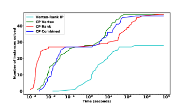
(a) Small feasible instances

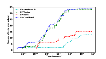
(b) Small infeasible instances

Figure 9: Solution times of the models for small instances.

Table LABEL:table:smallExact of Appendix E also reveals that $\mathbb{(CP^{RANK})}$ is able to solve instances with $D=0.7$ in less than a second, however, it begins to hit the time limit for $n\geq 35$ when $D=0.3$. For $D=0.5$, $\mathbb{(CP^{RANK})}$ is able to solve instances but is almost always outperformed by $\mathbb{(CP^{COMBINED})}$ and $\mathbb{(CP^{VERTEX})}$. We also remark that after 25 vertices, with $D=0.5$, the number of choice points for solving with $\mathbb{(CP^{RANK})}$ exceed one million for all but two instances.

Overall, we conclude lower density instances are more challenging for the CP models. However, high density ($D=0.7$) is trivial even with $60$ vertices. For these reasons, we focus on densities less than or equal to $0.5$, but increase the number of densities considered. Due to their poor performance, we exclude the IPs from further study. We now direct our focus to the CP models for medium-sized instances.

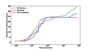
(a) Medium-sized feasible instances

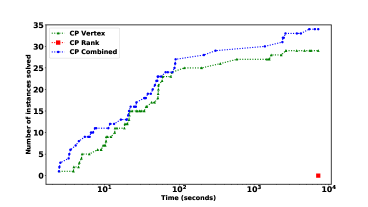
(b) Medium-sized infeasible instances

Figure 10: Solution times of the constraint programming models for medium-sized instances.

The performance profiles for the solutions times of different models on medium-sized instances are given in Figure 10 and the detailed results table can be found in Table LABEL:table:largeCP of Appendix E. We observe that $\mathbb{(CP^{RANK})}$ is outperformed by $\mathbb{(CP^{COMBINED})}$ and $\mathbb{(CP^{VERTEX})}$ in both the feasible and infeasible cases; it is unable to solve any infeasible instances. In the feasible case, $\mathbb{(CP^{VERTEX})}$ solves $6$ more instances than $\mathbb{(CP^{COMBINED})}$ within the time limit, however in the infeasible case, $\mathbb{(CP^{COMBINED})}$ solves $5$ more instances than $\mathbb{(CP^{VERTEX})}$ within the time limit. Overall, $\mathbb{(CP^{VERTEX})}$ is able to solve one more instance than $\mathbb{(CP^{COMBINED})}$ before the time limit is reached. We note however, that for medium-sized instances $25$ of the instances were unsolved by any method. For these medium-sized instances, those with $D=0.2$ or $D=0.5$ were all solved in less than $2$ minutes. The $D=0.3$ and $D=0.4$ instances are more difficult with only $13$ of $24$ instances with $D=0.4$ solved and no instances with $D=0.3$ and $n\geq 85$ solved. Thus there is still opportunity to improve the CP formulations.

Finally, we compare the best performing CP formulations, $\mathbb{(CP^{COMBINED})}$ and $\mathbb{(CP^{VERTEX})}$, with $\mathbb{(IP^{VR})}$ on the pseudo-protein instances. As seen in Figure 11, the results can be found in Tables LABEL:table:prot30 to LABEL:table:prot60 of Appendix E. We observe that $\mathbb{(CP^{VERTEX})}$ and $\mathbb{(CP^{COMBINED})}$ outperform $\mathbb{(IP^{VR})}$, which is only able to solve $39$ instances in total within the time limit. $\mathbb{(CP^{COMBINED})}$ has the best performance on these instances solving every instance in less than $32$ seconds. $\mathbb{(CP^{VERTEX})}$ is unable to solve $9$ instances before the time limit is hit. We observe that of the instances $\mathbb{(CP^{VERTEX})}$ is unable to solve, $8$ have $n\geq 40$ and they are those that have the highest density. Overall, we conclude that the CP formulations perform very well on pseudo-protein instances.

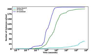
Figure 11: Solution times for pseudo-protein instances.

5.4 Preliminary Computational Study of Structural Findings

In this section, we present a preliminary study of the structural findings of Section 4. We implement them on $\mathbb{(CP^{COMBINED})}$ and test on the small random instances. In the worst case it takes 0.12 seconds to check for infeasibility and then apply domain reduction and symmetry breaking. For both the domain reduction and the symmetry breaking, we apply the infeasibility checks before solving. The infeasibility checks are able to prove four instances are infeasible without having to solve a mathematical program.

Solution times for $\mathbb{(CP^{COMBINED})}$ on small instances with domain reduction only and the symmetry breaking only, as well as both domain reduction and symmetry breaking together, and with no additions are shown in Figure 12. In total, for the set of $81$ small instances, Infeasibility Check 1 was able to solve two instances and Infeasibility Check 3 was also able to solve two instances. Domain Reduction Rule 1 was applied to $12$ instances. Finally, Symmetry Breaking Condition 4 was applied to $33$ instances, Symmetry Breaking Condition 5 was applied to $32$ instances, and Symmetry Breaking Condition 6 was applied to $37$ instances. None of the instances could be deemed infeasible using Infeasibility Checks 2 and 4. We were also unable to apply Domain Reduction Rule 2, and could not use Symmetry Breaking Conditions 1, 2, 3 for these instances.

We present the results in Table LABEL:table:enhance of Appendix E. We focus on small instances since we were unable to apply any of the findings other than arbitrary symmetry breaking to the medium-sized instances. We also see that the solution time with the addition of some combination of the structural strategies is decreased for $63$ of the $81$ instances. We believe this is because as $n$ increases, an instance is less likely to have degree less than $2K$, since $K$ is small with respect to $n$ and it is less likely that two vertices will have the same neighbourhoods. We observe that for feasible instances, symmetry breaking is slightly detrimental to the performance of $\mathbb{(CP^{COMBINED})}$ and that adding only domain reduction gives very similar results to no additions at all. However, for infeasible instances, we observe that domain reduction alone improves upon $\mathbb{(CP^{COMBINED})}$, and has similar performance to when both symmetry breaking and domain reduction are added to the model.

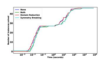
(a) Small feasible instances

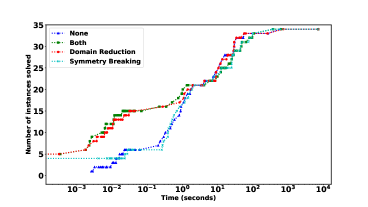
(b) Small infeasible instances

Figure 12: Solution times of the alternatives for structural findings.

For the majority of instances there exists an addition of one or more structural finding to the model that improves the solution time as compared to $\mathbb{(CP^{COMBINED})}$ on its own. Thus we conclude that the structural findings are beneficial for this data set. We also see that as the instance size increases we are unable to find these key structures in the graph. This motivates the future work of incorporating these structural insights into the CP search tree for further propagation opportunities and apply them at every node of the search tree to some subset of the order.

5.5 Preliminary Computational Study of Valid Inequalities

To provide insight into the class of valid inequalities using stable sets, (7) and (8), presented in Section 4.4, we study the impact of adding all possible valid inequalities to both $\mathbb{(CP^{RANK})}$ and $\mathbb{(CP^{COMBINED})}$ before solving. We use the Networkx Python package to enumerate all maximal stable sets for each small instance; the total time to enumerate these sets is $2.55$ seconds. We then add the valid inequalities (7) or (8) to the model as constraints using these stable sets and compare against the formulations without the valid inequalities. We remark that this is by no means a complete study of the impact of the valid inequalities but is meant to provide insight that even with a naive implementation there are cases where the valid inequalities are useful. The complete results table can be found in Table LABEL:table:VI of Appendix E

Figure 13(a) shows the results for small feasible instances. We observe that adding the valid inequalities was only slightly detrimental for both $\mathbb{(CP^{RANK})}$ and $\mathbb{(CP^{COMBINED})}$ and that the inequalities (7) have better performance than the inequalities (8). In the infeasible case, Figure 13(b), both forms of the valid inequalities increase the number of instances solved by $\mathbb{(CP^{RANK})}$ within the time limit and the speed at which they were solved. For $\mathbb{(CP^{COMBINED})}$ on the smallest infeasible instances, the formulations with valid inequalities (7) and (8) dominate the formulation without. In fact, the formulations with valid inequalities are able to solve some of these instances with $0$ choice points, which is notable. As the size of the instances grows, $\mathbb{(CP^{COMBINED})}$ without valid inequalities has better performance. This is most likely as a result of the larger instances having more stable sets and the subsequent models having a large number of constraints as a result.

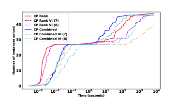
(a) Small feasible instances

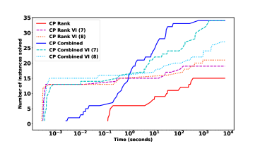
(b) Small infeasible instances

Figure 13: Solution times of the alternatives for valid inequalities (VI).

We conclude that in this preliminary implementation the valid inequalities are useful in small, low density instances and to improve $\mathbb{(CP^{RANK})}$ on infeasible instances. Future work on this topic includes further analysis to select a small enough subset of the stable sets that the number of constraints will not be too large and that will have a large impact on solution times. We remark however that the valid inequalities show promise given a more suitable implementation, such as a specialized propagator for the CP formulations.

6 Conclusion

We propose the first CP formulations for the CTOP and compare them against two existing IP formulations in the literature. Applying ideas from both the CP and IP literature, and by studying the structure of DMDGP orders, we introduce three classes of additions to formulations for CTOP, namely infeasibility checks, domain reduction, and symmetry breaking. We also provide the first class of valid inequalities for CTOP.

Our computational results show our models outperform the state-of-the-art IP formulations. They also indicate that the additions to the models based on structural findings are useful for infeasible instances, but may negatively impact the amount of time it takes to solve feasible instances. Nonetheless, they give important insight into the structure of CTOP and show promise for improvement and extension.

Acknowledgements

We are grateful to Leo Liberti for introducing us to the area of distance geometry and this topic in particular. We would also like to thank Jérémy Omer for kindly providing the pseudo-protein instances similar to those used in [18].

Appendix A Details of the Existing IP Models

Prior to this work, Cassioli et al. [1] present two IP formulations for CTOP.

A.1 The vertex-rank IP

Let $x_{vr}$ be a binary variable, which takes value $1$ if a vertex $v\in\mathcal{V}$ is receives rank $r\in[n-1]$ in the order, and $0$ otherwise. Since CTOP is a satisfiability problem, we are simply looking for a feasible order; there is no objective. The so-called vertex-rank IP formulation is as follows:

$$\mathbb{(IP^{VR})}:\ \sum_{r\in[n-1]}x_{vr}=1 \forall\ v\in\mathcal{V}$$ (9a)

$$\sum_{v\in\mathcal{V}}x_{vr}=1 \forall\ r\in[n-1]$$ (9b)

$$\sum_{u\in\mathcal{N}(v)}\sum_{j\in[r-1]}x_{uj}\geq rx_{vr} \forall\ v\in\mathcal{V},r\in[1,K-1]$$ (9c)

$$\sum_{u\in\mathcal{N}(v)}\sum_{j\in[r-K,r-1]}x_{uj}\geq Kx_{vr}\quad \forall\ v\in\mathcal{V},r\in[K,n-1]$$ (9d)

$$x_{vr}\in\{0,1\} \forall\ v\in\mathcal{V},r\in[n-1]$$ (9e)

Constraints (9a) and (9b) enforce a one-to-one assignment between the vertices and the ranks, so that each vertex appears exactly once in the order and that each rank gets exactly one vertex. Constraints (9c) enforce that there must be an initial clique of size $K$, i.e., that the vertices in positions $[K-1]$ are all adjacent to their predecessors. Constraints (9d) enforce each vertex with a rank in $[K,n-1]$ has at least $K$ contiguous predecessors. Finally, constraints (9e) ensure the binary domain of the vertex-rank variables.

Proof of Proposition 1. We claim that setting $x_{vr}=\frac{1}{n}$ for all $v\in\mathcal{V},r\in[n-1]$ always yields a feasible solution to the LP relaxation of $\mathbb{(IP^{VR})}$. We show the proposed solution satisfies all LP constraints. For constraints (9a), fixing $v\in\mathcal{V}$ gives

$$\sum_{r\in[n-1]}\frac{1}{n}=n\cdot\frac{1}{n}=1.$$

Similarly, for constraints (9b), fixing $r\in[n-1]$ gives

$$\sum_{v\in\mathcal{V}}\frac{1}{n}=|\mathcal{V}|\cdot\frac{1}{n}=n\cdot\frac{1}{n}=1.$$

For constraints (9c), for any $v\in\mathcal{V}$ and $r\in[1,K-1]$ we have

$$\sum_{u\in\mathcal{N}(v)}\sum_{j\in[r-1]}\frac{1}{n}\geq\sum_{j\in[r-1]}\frac{1}{n}=r\frac{1}{n}$$

where the inequality follows from $|\mathcal{N}(v)|\geq 1$ since $G$ is connected. Finally, for constraints (9d), for any $v\in\mathcal{V}$ and $r\in[K,n-1]$ we have

$$\sum_{u\in\mathcal{N}(v)}\sum_{j\in[r-K,r-1]}\frac{1}{n}\geq\sum_{j\in[r-K,r-1]}\frac{1}{n}=K\cdot\frac{1}{n}$$

again, due to $|\mathcal{N}(v)|\geq 1$ since G is connected.

Thus $x_{vr}=\frac{1}{n}$ satisfies all constraints and the LP relaxation is feasible. $\Box$

A.2 The clique digraph IP and its relaxation

As stated in Key Property 2, a DMDGP order is a series of overlapping induced $(K+1)$-cliques in $G$, which cover all the vertices and share $K$ vertices between adjacent pairs. Define a clique digraph $D=(\mathcal{O},\mathcal{A})$, where $\mathcal{O}$ is the index set of all ordered cliques $\{o_{j}\}_{j\in\mathcal{O}}$ of size $K+1$ in the input graph $G$, where $o_{j}=(v_{1}^{j},v_{2}^{j},\ldots,v_{K+1}^{j})$, i.e., represented simply by its ordered vertices. There is an arc $(o_{i},o_{j})\in\mathcal{A}$ between $o_{i},o_{j}\in\mathcal{O}$ if $v_{K+1}^{i}=v_{K}^{j}$, i.e., if the two cliques overlap by $K$ vertices and differ only by the first and the last vertex respectively. For instance, in the example given in Figure 2, there will be an arc in $\mathcal{A}$ between the vertices corresponding to the ordered 3-cliques $(v_{4},v_{2},v_{3})$ and $(v_{2},v_{3},v_{1})$. Let $\ell_{i}$ be the last vertex of a clique $o_{i}\in\mathcal{O}$. In this setting a DMDGP order is described by a path (of cliques) $P=(o_{1},o_{2},\ldots,o_{n-K})$ in $D$ where $\{v\in o_{c_{1}}\}\cup\{\ell_{i}:i\in[2,n-K]\}=\mathcal{V}$. That is, the initial clique and the last vertices of all other cliques cover $\mathcal{V}$. For instance, the DMDGP order given in Figure 2(b) is described by the path of cliques $o_{1}=(v_{4},v_{2},v_{3}),o_{2}=(v_{2},v_{3},v_{1}),o_{3}=(v_{3},v_{1},v_{5})$ and $o_{4}=(v_{1},v_{5},v_{0})$.

Define binary variables $x_{ij}=1$ if the arc $(i,j)\in\mathcal{A}$ is selected in the path solution $P$, $0$ otherwise. Let the binary variable $\gamma_{j}=1$ if $j\in\mathcal{O}$ is the first clique in $P$ and $\lambda_{j}=1$ if $j\in\mathcal{O}$ is the last clique in $P$. Define binary precedence variables $p_{uv}=1$ if $u\in\mathcal{V}$ precedes $v\in\mathcal{V}$ in the DMDGP order. Then the clique digraph IP formulation is as follows:

$$\mathbb{(IP^{CD})}:\min\ \sum_{(i,j)\in\mathcal{A}}x_{ij}$$ (10a)

s.t. $$\sum_{j\in\mathcal{O}}\gamma_{j}=1$$ (10b)

$$\sum_{j\in\mathcal{O}}\lambda_{j}=1$$ (10c)

$$\gamma_{i}+\sum_{\begin{subarray}{c}j\in\mathcal{O}\\ (j,i)\in\mathcal{A}\end{subarray}}x_{ji}=\lambda_{i}+\sum_{\begin{subarray}{c}j\in\mathcal{O}\\ (i,j)\in\mathcal{A}\end{subarray}}x_{ij}\quad \forall\ i\in\mathcal{O}$$ (10d)

$$\sum_{\begin{subarray}{c}j\in\mathcal{O}:\\ (i,j)\in\mathcal{A}\end{subarray}}x_{ij}\leq 1 \forall\ i\in\mathcal{O}$$ (10e)

$$\sum_{\begin{subarray}{c}j\in\mathcal{O}:\\ v\in o_{j}\end{subarray}}\gamma_{j}+\sum_{\begin{subarray}{c}(i,j)\in\mathcal{A}:\\ o_{j}\setminus o_{i}=\{v\}\end{subarray}}x_{ij}=1 \forall\ v\in\mathcal{V}$$ (10f)

$$p_{uv}+p_{vu}=1 \forall\ v,u\in\mathcal{V}\text{ s.t. }v\neq u$$ (10g)

$$p_{uv}+p_{vw}+p_{wu}\leq 2 \forall\ v,u,w\in\mathcal{V}\text{ s.t. }v\neq u\neq w$$ (10h)

$$p_{v_{k}^{i}v_{k+1}^{i}}\geq x_{ij} \forall\ (i,j)\in\mathcal{A},k\in[1,K]$$ (10i)

$$p_{v_{K+1}^{i}v}\geq x_{ij} \forall\ (i,j)\in\mathcal{A},v=o_{j}\setminus o_{i}$$ (10j)

$$p_{v^{i}_{k}v^{i}_{k+1}}\geq\gamma_{i}+\lambda_{i} \forall\ i\in\mathcal{O},k\in[1,K]$$ (10k)

$$\gamma^{i}\in\{0,1\} \forall\ i\in\mathcal{O}$$ (10l)

$$\lambda^{i}\in\{0,1\} \forall\ i\in\mathcal{O}$$ (10m)

$$x_{ij}\in\{0,1\} \forall\ (i,j)\in\mathcal{A}$$ (10n)

$$p_{uv}\in\{0,1\} \forall\ u,v\in\mathcal{V}$$ (10o)

Objective (10a) imposes that we will select the minimum number of arcs required to form the path $P$. Constraints (10b) and (10c) ensure there is exactly one initial clique and one last clique selected. Constraints (10d) ensure that flow balance holds in the path $P$ except at the first and last path vertices which have one arc out and one arc in respectively. These flow balance constraints also ensure a correct predecessor relationship between the cliques in $P$. Constraints (10e) ensure each clique has at most one successor, one if it is in the path and not the last clique and none otherwise. Constraints (10f) ensure that the cliques selected cover all the vertices in $\mathcal{V}$. Constraints (10g) and (10h) impose a linear order among vertex pairs and triplets. Constraints (10i), (10j), and (10k) ensure that each clique is ordered. Constraints (10i) impose that $v^{i}_{k}$ precedes vertex $v^{i}_{k+1}$ if ordered clique $i$ has an outgoing arc in the path solution $P$. Constraints (10j) ensure that if arc $(i,j)\in\mathcal{A}$ is selected in $P$, the vertex of $j$ not in $i$, $v$, is preceded by all other vertices of $j$ in $i$, which have been ordered by (10i). Constraints (10k) are similar to (10i), except they order the vertices of the first and last clique. Finally, constraints (10l), (10m), (10n), and (10o) enforce the binary domains of all variables.

$\mathbb{(IP^{CD})}$ is disadvantaged by the potential number of vertices in the clique digraph $D$, as the cardinality of $\mathcal{O}$ can be quite large even for relatively sparse graphs. To reduce the number of variables in $\mathbb{(IP^{CD})}$, Cassioli et al. [1] present a relaxation of the clique digraph formulation which considers unordered cliques. The idea is to relax the ordering constraints in the formulation and to solve this relaxation as a first check for the existence of a DMDGP order. In this case, the worst case number of vertices in $D$ can be reduced by a factor of $(K+1)!$. Let $\mathcal{O}$ now denote the set of unordered cliques of size $K+1$ in $G$. Let binary variable $z_{j}=1$ if the unordered clique $j\in\mathcal{O}$ is used in $P$. The unordered clique IP relaxation of $\mathbb{(IP^{CD})}$ is as follows:

$$\mathbb{(IP^{RELAX})}:\min\ \sum_{(i,j)\in\mathcal{A}}x_{ij}$$ (11a)

s.t. $$\eqref{IPcd:firstClique}-\eqref{IPcd:LOtriplets}$$ (11b)

$$p_{uv}\geq x_{ij} \forall\ (i,j)\in\mathcal{A},u\in o_{i},v=o_{j}\setminus o_{i}$$ (11c)

$$z_{j}\geq x_{ij} \forall\ (i,j)\in\mathcal{A}$$ (11d)

$$z_{i}\geq\gamma_{i} \forall\ i\in\mathcal{O}$$ (11e)

$$\sum_{\begin{subarray}{c}i\in\mathcal{O}:\\ v\in o_{i}\end{subarray}}z_{i}\leq K+1\quad \forall\ v\in\mathcal{V}$$ (11f)

$$\eqref{IPcd:domInitClique}-\eqref{IPcd:domArc}$$ (11g)

$$z_{i}\in\{0,1\} \forall\ i\in\mathcal{O}$$ (11h)

(11a) and(11b) are the same as in $\mathbb{(IP^{CD})}$. However, we have relaxed the clique ordering constraints, (10i)-(10k), so now constraints (11c) ensure we have that if arc $(i,j)\in\mathcal{A}$ is selected in $P$, all $u\in o_{i}$ precede vertex $v$, the only vertex of $j$ not in $i$. Constraints (11d) ensure we have correctly linked the arc variables and clique variables to the indicator $z_{j}$, so that it is $1$ if a clique is part of an arc selected in the solution path $P$, while the indicator for the first clique is activated through constraints (11e). The constraints (11f) impose that each vertex appears in at most $K+1$ cliques. These constraints are another relaxation, since to make it exact we would need to enforce that all vertices except the first and last $K$ appear in $K+1$ cliques; however this will require many more variables to express. Finally constraints (11g) and (11h) enforce the variable domains.

When a solution to $\mathbb{(IP^{RELAX})}$ is found, it must be verified as this solution does not necessarily yield a DMDGP order. The verification is a simple check to ensure the $p$ solution forms a DMDGP order. The strength in this formulation is that if $\mathbb{(IP^{RELAX})}$ is infeasible, there is no DMDGP order for the instance.

Appendix B Selected Proofs

B.1 Proof of Proposition 2

Proof.

Minimally, the vertex in position $0$ must be adjacent to $K$ vertices since it is in a $(K+1)$-clique, similarly for the vertex in position $n-1$. The vertex in position $1$ is in two $(K+1)$-cliques since it is in the initial clique but also is an adjacent predecessor of the vertex in position $K+1$; similarly for the vertex in position $n-2$. We extend this logic to all vertices in the order, noting that the centre $|\mathcal{V}|-2K$ vertices in the order, i.e., the ones in positions $[K,n-K-1]$, must all be in $2K$ cliques, as seen in Figure 14.

Figure 14: Minimum degree requirement for ranks in a DMDGP order.

This minimal case analysis gives a lower bound on the number of edges in a DMDGP order. For each vertex from position $0$ to position $n-1$ we sum over the minimum degree in $G$ to have a DMDGP order. Note that we divide by two to avoid double counting since the input graph is undirected.

$$\frac{1}{2}(K+(K+1)+(K+2)+\cdots+2K+\cdots+2K+\cdots+(K+2)+(K+1)+K)$$

$$=\frac{(|\mathcal{V}|-2K)2K+2\sum_{i=K}^{2K-1}i}{2}$$

$$=K(|\mathcal{V}|-2K)+\sum_{i=K}^{2K-1}i$$

$$=K(|\mathcal{V}|-2K)+\frac{1}{2}K(3K-1)$$

$$=\left(|\mathcal{V}|-\frac{1}{2}\right)K-\frac{1}{2}K^{2}$$

Thus the minimum number of edges for a DMDGP order is $\left(|\mathcal{V}|-\frac{1}{2}\right)K-\frac{1}{2}K^{2}$. ∎

B.2 Proof of Proposition 3

Proof.

We first show that there exists an instance for which (5) dominates (6). Consider the graph, $G_{1}$, shown in Figure 15(a) and let $K=3$. Let $\mathcal{S}_{1}=\{v_{1},v_{2},v_{3},v_{4},v_{5}\}$. Then $G_{1}[\mathcal{S}_{1}]=G_{1}$ does not have a DMDGP order due to Infeasibility Check 1, e.g., since $v_{3}$ cannot be in the initial clique and cannot have $K$ contiguous predecessors.

(a) $G_{1}$

(b) $G_{2}$

Figure 15: Graphs used to compare valid inequalities (5) and (6).

To find the inequality (5), we calculate $\max_{v\in\mathcal{S}_{1}}\delta^{miss}_{\mathcal{S}_{1}}(v)=\delta^{miss}_{\mathcal{S}_{1}}(v_{3})=3$ and find:

$$r_{max}-r_{min} \geq\max\{|\mathcal{S}_{1}|,\delta^{miss}_{\mathcal{S}_{1}}+K\}$$ (13a)

$$r_{max}-r_{min} \geq\max\{5,3+3\}$$ (13b)

$$r_{max}-r_{min} \geq 6$$ (13c)

The instance only has $5$ vertices in total, so this single inequality is enough to prove the instance does not have a DMDGP order. The largest stable set in the graph in Figure 15(a) has cardinality two; using any of these stable sets as $\mathcal{SS}_{1}$ makes the inequality (6)

$$r_{max}-r_{min} \geq(|\mathcal{SS}_{1}|-1)(K+1)$$ (14a)

$$r_{max}-r_{min} \geq(2-1)(3+1)$$ (14b)

$$r_{max}-r_{min} \geq 4$$ (14c)

which is not sufficient to prove the infeasibility of the instance. Thus (5) dominates (6) in this instance.
We now show that there exists an instance for which (6) dominates (5). Consider the graph, $G_{2}$, shown in Figure 15(b) and let $K=3$. A maximum stable set in $G_{2}$ is $\mathcal{SS}_{2}=\{u_{1},u_{3},u_{5}\}$, making the inequality (6):

$$r_{max}-r_{min} \geq(|\mathcal{SS}_{2}|-1)(K+1)$$ (15a)

$$r_{max}-r_{min} \geq(3-1)(3+1)$$ (15b)

$$r_{max}-r_{min} \geq 8$$ (15c)

Setting $\mathcal{S}_{2}=\mathcal{SS}_{2}$, then $G[\mathcal{S}_{2}]$ does not have a DMDGP order due to Infeasibility Check 1.We calculate $\max_{u\in\mathcal{S}_{2}}\delta^{miss}_{\mathcal{S}_{2}}(u)=2$ and find

$$r_{max}-r_{min} \geq\max\{|\mathcal{S}_{2}|,\delta^{miss}_{\mathcal{S}_{2}}+K\}$$ (16a)

$$r_{max}-r_{min} \geq\max\{3,2+3\}$$ (16b)

$$r_{max}-r_{min} \geq 5$$ (16c)

Thus (6) dominates (5), and we may conclude that (5) and (6) are incomparable.

∎

B.3 Proof of Proposition 4

Proof.

Let the vertices in the wheel be indexed as in Figure 8, i.e., the centre vertex has index 0, while the ones in the peripheral cycle are indexed from $[1,n]$ counter clock-wise starting at an arbitrary one.

• Case 1: When $n$ is odd, a maximum stable set in $W_{n}$ is $\{1,3,\ldots,n-2\}$ with size $\frac{n-1}{2}$. For the right-hand side of the inequality in Infeasibility Check 5 to hold, we need

  $$\frac{n-1}{2}\geq\frac{n}{K+1}+1$$

  $$\frac{n}{2}-\frac{n}{K+1}\geq\frac{1}{2}$$

  $$n\left(\frac{1}{2}-\frac{1}{K+1}\right)\geq\frac{1}{2}$$

  $$n\geq\frac{K+1}{K-1}.$$

• Case 2: Similarly, when $n$ is even, a maximum stable set in $W_{n}$ is $\{1,3,\ldots,n-3\}$ with size $\frac{n}{2}$. So we need

  $$\frac{n}{2}\geq\frac{n}{K+1}+1$$

  $$n\left(\frac{1}{2}-\frac{1}{K+1}\right)\geq 1$$

  $$n\geq 2\frac{K+1}{K-1}.$$

Thus the inequalities hold. ∎

Appendix C Example

Example 10.

We will demonstrate the strength of symmetry breaking on the graph in Figure 16 with $K=2$.

Figure 16: A graph instance which is feasible for CTOP with $K=2$.

This instance has $12$ feasible DMDGP orders:

$$(v_{4},v_{3},v_{2},v_{1},v_{0},v_{5}) (v_{5},v_{0},v_{1},v_{2},v_{3},v_{4}) (v_{4},v_{3},v_{2},v_{5},v_{0},v_{1})$$

$$(v_{1},v_{0},v_{5},v_{2},v_{3},v_{4}) (v_{4},v_{2},v_{3},v_{1},v_{5},v_{0}) (v_{0},v_{5},v_{1},v_{3},v_{2},v_{4})$$

$$(v_{4},v_{3},v_{2},v_{1},v_{5},v_{0}) (v_{0},v_{5},v_{1},v_{2},v_{3},v_{4}) (v_{4},v_{2},v_{3},v_{5},v_{1},v_{0})$$

$$(v_{0},v_{1},v_{5},v_{3},v_{2},v_{4}) (v_{4},v_{3},v_{2},v_{5},v_{1},v_{0}) (v_{0},v_{1},v_{5},v_{2},v_{3},v_{4})$$

We begin by noticing that $\mathcal{V}^{d[2,2]}=\{v_{4}\}$ so we fix $r_{v_{4}}=0$ and eliminate half the orders, leaving the orders:

$$(v_{4},v_{3},v_{2},v_{1},v_{0},v_{5}) (v_{4},v_{2},v_{3},v_{1},v_{5},v_{0}) (v_{4},v_{3},v_{2},v_{5},v_{0},v_{1})$$

$$(v_{4},v_{3},v_{2},v_{1},v_{5},v_{0}) (v_{4},v_{3},v_{2},v_{5},v_{1},v_{0}) (v_{4},v_{2},v_{3},v_{5},v_{1},v_{0})$$

There are no stable sets meeting Symmetry Breaking Condition 2, and the only clique meeting Symmetry Breaking Condition 3 is $\{v_{1},v_{5}\}$. Thus we enforce $r_{v_{1}}<r_{v_{5}}$ and eliminate another three orders, leaving three remaining orders:

$$(v_{4},v_{3},v_{2},v_{1},v_{0},v_{5}) (v_{4},v_{3},v_{2},v_{1},v_{5},v_{0}) (v_{4},v_{3},v_{2},v_{5},v_{0},v_{1}).$$

Since we have found a clique in Symmetry Breaking Condition 3, we first examine Symmetry Breaking Condition 5. Beginning with $\mathcal{K}=\{v_{1},v_{5}\}$ and $v=v_{2}$, we have

$$(\mathcal{N}(v_{2})\cup\{v_{2}\})\setminus(\mathcal{N}(\{v_{1},v_{5}\})\cup\{v_{1},v_{5}\})=\{v_{0},v_{1},v_{2},v_{3},v_{4},v_{5}\}\setminus\{v_{0},v_{1},v_{2},v_{3},v_{5}\}=\{v_{4}\}$$

so $w=v_{4}$ and we can add the following logical constraints:

$$|r_{v_{2}}-r_{v_{4}}|\geq 3\implies r_{v_{2}}<r_{v_{5}}$$

$$|r_{v_{2}}-r_{v_{4}}|\geq 3\implies r_{v_{2}}<r_{v_{1}}$$

In fact, the latter suffices since we have already added $r_{v_{1}}<r_{v_{5}}$. Unfortunately this does not remove any solutions from the pool. We now try $\mathcal{K}=\{v_{0}\}$ and $v=v_{5}$. In this case we have $w=v_{3}$ and add

$$|r_{v_{5}}-r_{v_{3}}|\geq 3\implies r_{v_{5}}<r_{v_{0}}$$

which removes a further order, yielding the remaining orders:

$$(v_{4},v_{3},v_{2},v_{1},v_{5},v_{0}) (v_{4},v_{3},v_{2},v_{5},v_{0},v_{1}).$$

Finally, we extend $\mathcal{K}=\{v_{3}\}$ using $v=2$, giving $w=v_{0}$ and the logical constraint:

$$|r_{v_{2}}-r_{v_{0}}|\geq 3\implies r_{v_{2}}<r_{v_{3}}$$

Thus symmetry breaking has reduced the solution space to a single DMDGP order:

$$(v_{4},v_{3},v_{2},v_{5},v_{0},v_{1})$$

Appendix D Summary of the paper

Table LABEL:table:DMDGPsummary provides a summary of the models from the literature as well as all of our proposed formulations and structural insights.

Appendix E DMDGP Results

We provide the following tables:

• Table LABEL:table:smallExact compares the integer programming formulations from the literature [1], namely the vertex-rank formulation $\mathbb{(IP^{VR})}$ and the clique digraph formulation $\mathbb{(IP^{CD})}$, with the newly proposed constraint programming formulations, namely the rank-based primal formulation $\mathbb{(CP^{RANK})}$, the vertex-based dual formulation $\mathbb{(CP^{VERTEX})}$ and the combined formulation $\mathbb{(CP^{COMBINED})}$ on the small instances for a variety of densities with $K=3$.

• Table LABEL:table:largeCP compares the CP formulations $\mathbb{(CP^{RANK})}$, $\mathbb{(CP^{VERTEX})}$, and $\mathbb{(CP^{COMBINED})}$ on the medium-sized instances for low to medium densities with $K=3$.

• Table LABEL:table:CDrelax compares the IP Clique Digraph formulations $\mathbb{(IP^{CD})}$ and $\mathbb{(IP^{RELAX})}$ on small instances with $K=3$.

• Tables LABEL:table:prot30, LABEL:table:prot40, LABEL:table:prot50, and LABEL:table:prot60 compare the $\mathbb{(IP^{VR})}$, $\mathbb{(CP^{VERTEX})}$, and $\mathbb{(CP^{COMBINED})}$ formulations with $K=3$ on pseudo-protein instances with $30,40,50,$ and $60$ vertices respectively.

• Table LABEL:table:enhance compares the $\mathbb{(CP^{COMBINED})}$ formulation with $K=3$, with and without the additions from the structural analysis, on small instances. It also gives the rule that was applied and to how many vertices or sets using the following conventions:

  • $[\text{Inf}r]$ refers to Infeasibility Check $r$, either 1 or 3.

  • $[\text{DR}r]$ refers to Domain Reduction Rule 1 which has been applied to $r$ vertices.

  • $[\text{E}\mathcal{SS}s]$ refers to Symmetry Breaking Condition 4 which has been applied to $s$ stable sets.

  • $[\text{E}\mathcal{K}c]$ refers to Symmetry Breaking Condition 5 which has been applied to $c$ cliques

  • $[\text{Arb}]$ refers to an arbitrary ordering on two vertices, as in Symmetry Breaking Condition 6.

  We note that Infeasibility Checks 2 and 4, Domain Reduction Rule 2, and Symmetry Breaking Conditions 1, 2, 3 are excluded from the table since they were never applied.

• Table LABEL:table:VI compares $\mathbb{(CP^{RANK})}$ and $\mathbb{(CP^{COMBINED})}$ with valid inequalities in the form (7) and (8) and without valid inequalities. Valid inequalities are generated for every stable set in each instance and added before solving.

• Table LABEL:table:K4 compares the vertex-rank formulation $\mathbb{(IP^{VR})}$ with CP formulations $\mathbb{(CP^{RANK})}$, $\mathbb{(CP^{VERTEX})}$, and $\mathbb{(CP^{COMBINED})}$ on the small instance with $K=4$.

• Table LABEL:table:K5 compares the vertex-rank formulation $\mathbb{(IP^{VR})}$ with CP formulations $\mathbb{(CP^{RANK})}$, $\mathbb{(CP^{VERTEX})}$, and $\mathbb{(CP^{COMBINED})}$ on the small instance with $K=5$.

For the instances, we have

• “Status”: Feasibility status of the instance; “Feas.” and “Infeas.” if it is proven to be feasible and infeasible by any of the methods, respectively, “Unsol.” otherwise as it is not solved by any method.

In particular, for random instances we have

• “$n$”: The number of vertices in the input graph.

  • $n\in\{20,25,\ldots,60\}$ for the small instances.

  • $n\in\{65,70,\ldots,100\}$ for the medium-sized instances.

• “$D$”: The edge density of the input graph.

  • $D\in\{0.3,0.5,0.7\}$ for the small instances.

  • $D\in\{0.2,0.3,0.4,0.5\}$ for the medium-sized instances.

• “Inst.”: The assigned instance number from $\{1,2,3\}$ for each $(n,D)$ combination.

For pseudo-protein instances we have

• “Protein Inst.”: the Protein Data Bank protein which was modified to create the instance.

• “Ratio”: the approximate average edge to vertex ratio of the instance.

We also have

• “Time”: Solution time in seconds if the instance is solved in the given time limit, “TL” if the instance hit the time limit, “MEM” if the instance hit the memory limit.

• “BB Nodes”: The number of branch-and-bound nodes explored (for the IP formulations); exact if it is less than one thousand, lower bound rounded to the closest million otherwise where a single decimal point is used up to between one million for a better accuracy.

• “Ch.Pts.”: The number of choice points (for the CP formulations); the number convention is the same as the “BB Nodes”.

• ”Solved”: indicates if a feasible solution was found.

• “DMDGP found”: “Yes” if the feasible solution is a DMDGP order, “No” otherwise.

• “# cliques”: the number of ordered and unordered cliques for $\mathbb{(IP^{CD})}$ and $\mathbb{(IP^{RELAX})}$ respectively.

Table 2: Integer programming and constraint programming results for small instances

				$\mathbb{(IP^{VR})}$		$\mathbb{(IP^{CD})}$		$\mathbb{(CP^{RANK})}$		$\mathbb{(CP^{VERTEX})}$		$\mathbb{(CP^{COMBINED})}$
$n$	$D$	Inst.	Status	Time	BB Nodes	Time	BB Nodes	Time	Ch.Pts.	Time	Ch.Pts.	Time	Ch.Pts.
20	0.3	1	Infeas.	41.43	5981	0.00	0	0.16	8937	0.10	1987	0.01	72
		2	Infeas.	0.01	0	0.00	0	0.13	7286	0.01	130	0.00	17
		3	Infeas.	29.08	5188	0.00	0	0.15	8255	0.01	122	0.00	20
	0.5	1	Infeas.	132.53	52865	4.13	0	0.21	10850	0.80	9705	0.91	9423
		2	Infeas.	156.95	79733	5.66	0	0.13	7408	0.65	8402	0.29	3909
		3	Infeas.	27.35	8844	1.86	0	0.15	8279	0.78	8836	0.20	2519
	0.7	1	Feas.	0.18	0	TL	0	0.00	55	0.02	621	0.01	129
		2	Feas.	0.22	125	TL	0	0.00	57	0.01	137	0.00	30
		3	Feas.	0.27	112	TL	0	0.00	15	0.01	128	0.00	65
25	0.3	1	Infeas.	0.02	0	0.00	0	10.35	417400	0.21	3779	0.02	194
		2	Infeas.	105.34	6376	0.00	0	8.86	382191	0.23	4184	0.02	160
		3	Infeas.	59.15	5303	0.00	0	6.55	276282	0.01	184	0.01	123
	0.5	1	Infeas.	3835.96	882598	0.03	0	34.84	$>$ 1.1M	22.00	195704	0.23	2415
		2	Infeas.	TL	$>$ 1.8M	962.72	0	114.68	$>$ 3.1M	33.40	328076	16.01	100057
		3	Infeas.	TL	$>$ 1.8M	632.05	0	31.15	$>$ 1.0M	7.76	57986	7.47	44433
	0.7	1	Feas.	5.70	3902	MEM	-	0.00	39	0.02	578	0.01	45
		2	Feas.	0.56	251	MEM	-	0.00	109	0.00	24	0.00	30
		3	Feas.	0.43	39	MEM	-	0.00	26	0.01	171	0.01	141
30	0.3	1	Infeas.	843.31	52684	0.00	0	308.12	$>$ 9.2M	0.25	3204	0.45	3225
		2	Infeas.	639.51	33523	0.00	0	368.72	$>$ 9.6M	0.43	4152	0.33	2191
		3	Infeas.	531.50	31092	0.00	0	251.35	$>$ 7.3M	0.43	4874	0.50	3429
	0.5	1	Feas.	TL	$>$ 1.2M	TL	0	66.41	$>$ 2.8M	67.56	613865	53.36	299863
		2	Infeas.	TL	954489	TL	0	TL	$>$ 102M	TL	$>$27M	601.23	$>$2.7M
		3	Feas.	TL	$>$ 1.2M	TL	0	89.47	$>$ 4.3M	2.07	24663	4.60	29699
	0.7	1	Feas.	0.72	203	MEM	-	0.00	33	0.01	147	0.02	195
		2	Feas.	1.16	540	MEM	-	0.00	112	0.00	34	0.01	27
		3	Feas.	2.24	1285	MEM	-	0.00	33	0.00	33	0.03	379
35	0.3	1	Infeas.	TL	463579	0.00	0	TL	$>$ 308M	1.17	7248	0.59	3517
		2	Infeas.	TL	244370	0.00	0	TL	$>$ 363M	0.55	4819	0.89	4033
		3	Infeas.	TL	529463	0.00	0	TL	$>$ 267M	0.55	4341	0.81	4043
	0.5	1	Feas.	TL	$>$ 1.4M	TL	0	279.32	$>$ 13M	2.95	30082	7.14	40622
		2	Feas.	TL	$>$ 1.0M	TL	0	26.89	$>$ 1.2M	45.94	526013	16.28	113300
		3	Feas.	TL	$>$ 1.0M	TL	0	4825.99	$>$ 271M	39.62	383353	TL	$>$32M
	0.7	1	Feas.	1.33	95	MEM	-	0.00	39	0.01	34	0.01	34
		2	Feas.	1.35	166	MEM	-	0.01	267	0.00	33	0.03	273
		3	Feas.	1.58	74	MEM	-	0.00	37	0.00	33	0.01	30
40	0.3	1	Infeas.	TL	253348	0.00	0	TL	$>$ 323M	1.58	7482	2.04	6156
		2	Infeas.	TL	179520	0.00	0	TL	$>$ 41M	0.87	5143	1.41	4789
		3	Infeas.	TL	215387	0.00	0	TL	$>$ 40M	1.52	8490	1.07	4191
	0.5	1	Feas.	TL	$>$ 1.0M	MEM	-	557.97	$>$ 24M	6.58	56710	266.57	$>$1.31M
		2	Feas.	TL	878086	MEM	-	37.55	$>$ 1.6M	11.35	111152	9.10	51413
		3	Feas.	TL	831307	MEM	-	35.85	$>$ 1.5M	6.93	66262	23.88	130898
	0.7	1	Feas.	1.33	0	MEM	-	0.00	36	0.05	577	0.02	166
		2	Feas.	2.77	123	MEM	-	0.00	44	0.00	39	0.01	34
		3	Feas.	2.21	50	MEM	-	0.00	176	0.09	1074	0.01	68
45	0.3	1	Infeas.	TL	167176	0.01	0	TL	$>$ 298M	6.92	21970	8.70	18790
		2	Infeas.	TL	99401	0.01	0	TL	$>$ 42M	4.74	17489	1.19	3473
		3	Infeas.	TL	119535	1.89	0	TL	$>$ 41M	4.76	19927	1.70	5194
	0.5	1	Feas.	242.69	10702	MEM	-	9.75	430149	4.61	41180	3.56	16486
		2	Feas.	TL	565030	MEM	-	237.99	$>$ 10M	12.61	103490	3.85	18158
		3	Feas.	TL	676199	MEM	-	33.00	$>$ 1.4M	4.52	38613	3.37	16901
	0.7	1	Feas.	4.04	132	MEM	-	0.00	41	0.01	47	0.01	39
		2	Feas.	1.53	0	MEM	-	0.00	40	0.01	47	0.01	50
		3	Feas.	2.86	10	MEM	-	0.00	46	0.03	452	0.02	129
50	0.3	1	Infeas.	TL	68691	0.02	0	TL	$>$ 280M	12.36	32724	4.32	9124
		2	Infeas.	TL	103348	7.04	0	TL	$>$ 37M	7.36	23010	13.50	27987
		3	Infeas.	TL	69546	0.02	0	TL	$>$ 37M	14.36	38069	10.53	19301
	0.5	1	Feas.	TL	283084	MEM	-	287.47	$>$ 12M	16.59	113189	42.87	169360
		2	Feas.	TL	554285	MEM	-	32.18	$>$ 1.3M	0.59	4490	1.63	7874
		3	Feas.	TL	473504	MEM	-	153.82	$>$ 6.3M	7.04	50776	7.83	31997
	0.7	1	Feas.	6.59	273	MEM	-	0.00	52	0.01	51	0.01	47
		2	Feas.	9.27	195	MEM	-	0.00	46	0.01	48	0.05	315
		3	Feas.	9.01	201	MEM	-	0.00	48	0.06	669	0.03	190
55	0.3	1	Infeas.	TL	49459	14.13	0	TL	$>$ 261M	13.78	29494	28.38	43711
		2	Infeas.	TL	51372	0.03	0	TL	$>$ 32M	17.57	36651	30.21	44814
		3	Infeas.	TL	46087	0.03	0	TL	$>$ 32M	16.85	31236	29.51	43579
	0.5	1	Feas.	TL	475709	MEM	-	158.49	$>$ 6.2M	23.19	155633	20.74	80931
		2	Feas.	TL	483159	MEM	-	1.92	73055	7.62	49245	17.80	65528
		3	Feas.	TL	390397	MEM	-	52.05	$>$ 1.9M	5.85	32292	41.29	164410
	0.7	1	Feas.	16.19	141	MEM	-	0.00	359	0.09	804	0.02	77
		2	Feas.	14.80	439	MEM	-	0.00	72	0.20	1801	0.02	110
		3	Feas.	11.65	193	MEM	-	0.00	53	0.01	52	0.01	50
60	0.3	1	Infeas.	TL	24403	4061.37	0	TL	$>$ 268M	92.01	147378	57.55	66028
		2	Infeas.	TL	14867	26.81	0	TL	$>$ 34M	23.44	44252	34.55	43375
		3	Infeas.	TL	18187	0.07	0	TL	$>$ 42M	73.24	135352	11.73	16208
	0.5	1	Feas.	TL	349369	MEM	-	92.38	$>$ 3.4M	14.37	85998	9.01	30615
		2	Feas.	TL	141418	MEM	-	117.15	$>$ 5.5M	9.27	59659	25.93	91975
		3	Feas.	TL	279238	MEM	-	4.05	191858	27.21	174109	45.13	158247
	0.7	1	Feas.	34.36	180	MEM	-	0.00	56	0.03	212	0.06	277
		2	Feas.	25.75	596	MEM	-	0.00	69	0.03	221	0.02	102
		3	Feas.	35.99	278	MEM	-	0.00	61	0.01	60	0.03	107

Table 3: Constraint programming results for medium-sized instances

				$\mathbb{(CP^{RANK})}$		$\mathbb{(CP^{VERTEX})}$		$\mathbb{(CP^{COMBINED})}$
$n$	$D$	Inst.	Status	Time	Ch.Pts.	Time	Ch.Pts.	Time	Ch.Pts.
65	0.2	1	Infeas.	TL	265M	4.60	12430	2.46	3781
		2	Infeas.	TL	266M	5.01	12963	3.50	4263
		3	Infeas.	TL	267M	8.09	16647	2.49	3574
	0.3	1	Infeas.	TL	297M	352.77	428908	86.21	79144
		2	Infeas.	TL	294M	2659.91	3.8M	22.35	23589
		3	Infeas.	TL	295M	116.46	149767	213.19	200152
	0.4	1	Unsol.	TL	292M	TL	$>$24M	TL	$>$14M
		2	Unsol.	TL	294M	TL	$>$26M	TL	$>$14M
		3	Unsol.	TL	293M	TL	$>$22M	TL	$>$13M
	0.5	1	Feas.	27.63	$>$1.2M	3.84	22151	7.75	23745
		2	Feas.	319.69	$>$13M	46.63	248767	19.81	60984
		3	Feas.	73.69	$>$3.1M	20.23	120980	70.21	229712
70	0.2	1	Infeas.	TL	246M	2.47	6133	7.46	10838
		2	Infeas.	TL	249M	3.89	8936	3.32	4681
		3	Infeas.	TL	247M	9.58	19539	4.11	4635
	0.3	1	Infeas.	TL	271M	TL	$>$8.4M	2424.76	$>$2.3M
		2	Infeas.	TL	277M	587.53	676349	65.50	59863
		3	Infeas.	TL	268M	1692.80	$>$2.2M	304.72	262913
	0.4	1	Unsol.	TL	274M	TL	22M	TL	$>$14M
		2	Feas.	TL	276M	1596.55	$>$4.9M	6490.16	$>$12M
		3	Unsol.	TL	274M	TL	$>$21M	TL	$>$13M
	0.5	1	Feas.	53.29	$>$2.2M	19.95	95724	6.06	16960
		2	Feas.	15.79	657645	11.01	54130	51.68	146234
		3	Feas.	153.93	$>$6.4M	23.30	108045	26.21	67902
75	0.2	1	Infeas.	TL	232M	13.70	20500	4.54	5683
		2	Infeas.	TL	228M	21.23	39721	2.57	3272
		3	Infeas.	TL	234M	13.82	23875	3.38	4321
	0.3	1	Infeas.	TL	250M	TL	$>$7.3M	2388.75	$>$2.0M
		2	Infeas.	TL	253M	TL	$>$7.6M	2627.21	$>$2.2M
		3	Infeas.	TL	249M	TL	$>$7.8M	1393.82	$>$1.1M
	0.4	1	Unsol.	TL	256M	TL	$>$17M	TL	$>$11M
		2	Feas.	TL	255M	4720.92	$>$13M	TL	$>$13M
		3	Unsol.	TL	258M	TL	$>$21M	TL	$>$13M
	0.5	1	Feas.	52.18	2.1M	8.98	36417	13.41	32718
		2	Feas.	30.63	$>$12.M	6.24	26811	25.00	65955
		3	Feas.	29.06	$>$1.1M	10.25	44649	52.63	137809
80	0.2	1	Infeas.	TL	217M	10.54	14933	21.26	22259
		2	Infeas.	TL	208M	4.92	7799	11.85	13623
		3	Infeas.	TL	217M	10.48	15404	16.55	18362
	0.3	1	Unsol.	TL	235M	TL	6.8M	TL	$>$5.7M
		2	Unsol.	TL	236M	TL	6.8M	TL	$>$5.5M
		3	Infeas.	TL	234M	TL	$>$7.1M	5465.09	$>$4.0M
	0.4	1	Feas.	TL	242M	198.71	546437	TL	$>$11M
		2	Unsol.	TL	240M	TL	$>$17M	TL	$>$11M
		3	Unsol.	TL	241M	TL	$>$20M	TL	$>$11M
	0.5	1	Feas.	8.63	325945	30.99	118909	7.02	15534
		2	Feas.	9.16	366384	4.49	16480	19.60	44067
		3	Feas.	22.14	835657	12.22	43777	34.61	76300
85	0.2	1	Infeas.	TL	198M	21.74	26137	6.59	5974
		2	Infeas.	TL	195M	18.74	25012	33.92	30334
		3	Infeas.	TL	194M	21.51	27435	5.46	5022
	0.3	1	Unsol.	TL	220M	TL	$>$7.2M	TL	$>$5.3M
		2	Unsol.	TL	218M	TL	$>$6.5M	TL	$>$5.2M
		3	Unsol.	TL	218M	TL	$>$7.8M	TL	$>$5.6M
	0.4	1	Unsol.	TL	226M	TL	1.78E+07	TL	$>$10M
		2	Feas.	TL	225M	2666.80	$>$6.8M	3726.22	$>$5.7M
		3	Feas.	TL	227M	TL	$>$13M	2492.79	$>$3.7M
	0.5	1	Feas.	25.75	958375	18.42	44029	6.32	13251
		2	Feas.	16.45	604637	33.96	80773	2.26	5249
		3	Feas.	25.58	916732	9.04	20806	35.66	78389
90	0.2	1	Infeas.	TL	183M	52.08	40320	20.69	17215
		2	Infeas.	TL	181M	60.12	50875	51.51	39634
		3	Infeas.	TL	186M	42.69	32850	26.70	20576
	0.3	1	Unsol.	TL	201M	TL	$>$5.3M	TL	$>$5.3M
		2	Unsol.	TL	201M	TL	$>$5.8M	TL	$>$4.7M
		3	Unsol.	TL	185M	TL	$>$6.6M	TL	$>$5.4M
	0.4	1	Feas.	TL	197M	5786.42	$>$13M	TL	$>$10M
		2	Feas.	TL	192M	2306.22	$>$5.1M	TL	$>$8.7M
		3	Feas.	TL	197M	1577.54	$>$3.3M	TL	$>$9.6M
	0.5	1	Feas.	35.62	$>$1.2M	27.13	91993	24.86	48101
		2	Feas.	12.85	450199	2.12	6440	41.59	76803
		3	Feas.	197.06	6.7M	14.68	42569	80.77	160588
95	0.2	1	Infeas.	TL	168M	52.59	48464	49.39	33305
		2	Infeas.	TL	178M	35.94	34804	37.93	27387
		3	Infeas.	TL	187M	58.82	60428	47.19	34976
	0.3	1	Unsol.	TL	182M	TL	$>$5.8M	TL	$>$4.8M
		2	Unsol.	TL	190M	TL	6.4M	TL	$>$4.8M
		3	Unsol.	TL	189M	TL	$>$5.7M	TL	$>$4.8M
	0.4	1	Feas.	TL	181M	1482.63	$>$2.8M	TL	$>$9.0M
		2	Feas.	TL	180M	TL	$>$14M	TL	$>$9.1M
		3	Feas.	TL	177M	TL	$>$14M	TL	$>$8.9M
	0.5	1	Feas.	0.75	18309	1.53	4223	6.74	11955
		2	Feas.	15.60	407153	77.00	246670	26.07	45377
		3	Feas.	2.62	65770	26.97	89663	11.23	18867
100	0.2	1	Infeas.	TL	141M	52.52	49457	44.07	30257
		2	Infeas.	TL	171M	51.74	45165	88.06	56078
		3	Infeas.	TL	169M	79.87	55536	89.22	48202
	0.3	1	Unsol.	TL	178M	TL	$>$5.7M	TL	$>$4.5M
		2	Unsol.	TL	177M	TL	$>$5.7M	TL	$>$4.6M
		3	Unsol.	TL	177M	TL	$>$5.5M	TL	$>$4.4M
	0.4	1	Feas.	TL	193M	3712.55	$>$7.4M	TL	$>$8.5M
		2	Unsol.	TL	186M	TL	$>$1.2M	TL	$>$8.5M
		3	Feas.	TL	192M	5567.75	$>$1.1M	4220.47	$>$5.0M
	0.5	1	Feas.	27.81	856316	9.95	27349	50.73	81993
		2	Feas.	12.77	389470	36.75	119129	3.51	5929
		3	Feas.	25.64	782540	29.37	79750	56.99	95817

Table 4: Results for $\mathbb{(IP^{CD})}$ and $\mathbb{(IP^{RELAX})}$ on small instances.

				$\mathbb{(IP^{RELAX})}$		# Cliques		Time		BB Nodes
$n$	$D$	Inst.	Status	Solved	DMDGP found	$\mathbb{(IP^{CD})}$	$\mathbb{(IP^{RELAX})}$	$\mathbb{(IP^{CD})}$	$\mathbb{(IP^{RELAX})}$	$\mathbb{(IP^{CD})}$	$\mathbb{(IP^{RELAX})}$
20	0.3	1	Infeas.	-	-	168	7	0.00	0.00	0	0
		2	Infeas.	-	-	48	2	0.00	0.00	0	0
		3	Infeas.	-	-	96	4	0.00	0.00	0	0
	0.5	1	Infeas.	-	-	1656	69	4.13	2.08	0	0
		2	Infeas.	-	-	1920	80	5.66	1.83	0	0
		3	Infeas.	-	-	1272	53	1.86	0.00	0	0
	0.7	1	Feas.	Yes	No	13872	578	TL	5308.77	0	6287
		2	Feas.	Yes	No	12000	500	TL	2217.26	0	7172
		3	Feas.	Yes	No	13872	578	TL	2105.65	0	3579
25	0.3	1	Infeas.	-	-	288	12	0.00	0.00	0	0
		2	Infeas.	-	-	216	9	0.00	0.00	0	0
		3	Infeas.	-	-	96	4	0.00	0.00	0	0
	0.5	1	Infeas.	-	-	4776	199	0.03	0.01	0	0
		2	Infeas.	-	-	4368	182	962.72	4095.70	0	7968
		3	Infeas.	-	-	3960	165	632.05	TL	0	18996
	0.7	1	Feas.	No	-	36360	1515	MEM	TL	-	287
		2	Feas.	No	-	34344	1431	MEM	TL	-	180
		3	Feas.	Yes	No	32856	1369	MEM	4536.87	-	333
30	0.3	1	Infeas.	-	-	264	11	0.00	0.01	0	0
		2	Infeas.	-	-	240	10	0.00	0.01	0	0
		3	Infeas.	-	-	360	15	0.00	0.01	0	0
	0.5	1	Feas.	No	-	10896	454	TL	TL	0	3742
		2	Unsol.	-	-	9264	386	TL	TL	0	3293
		3	Feas.	-	-	9960	415	TL	TL	0	2866
	0.7	1	Feas.	No	-	73872	3078	MEM	TL	-	12
		2	Feas.	No	-	72888	3037	MEM	TL	-	6
		3	Feas.	No	-	76488	3187	MEM	TL	-	3
35	0.3	1	Infeas.	-	-	864	36	0.00	0.01	0	0
		2	Infeas.	-	-	576	24	0.00	0.01	0	0
		3	Infeas.	-	-	696	29	0.00	0.01	0	0
	0.5	1	Feas.	No	-	18888	787	TL	TL	0	1457
		2	Feas.	No	-	21408	892	TL	TL	0	1828
		3	Feas.	No	-	20304	846	TL	TL	0	605
	0.7	1	Feas.	No	-	143616	5984	MEM	TL	-	0
		2	Feas.	No	-	151056	6294	MEM	TL	-	0
		3	Feas.			140976	5874	MEM	TL	-	0
40	0.3	1	Infeas.	-	-	1776	74	0.00	0.01	0	0
		2	Infeas.	-	-	816	34	0.00	0.01	0	0
		3	Infeas.	-	-	1344	56	0.00	0.01	0	0
	0.5	1	Feas.	No	-	34680	1445	MEM	TL	-	56
		2	Feas.	No	-	37056	1544	MEM	TL	-	72
		3	Feas.	No	-	35160	1465	MEM	TL	-	48
	0.7	1	Feas.	No	-	250608	10442	MEM	TL	-	0
		2	Feas.	No	-	265440	11060	MEM	TL	-	0
		3	Feas.	No	-	256224	10676	MEM	TL	-	0
45	0.3	1	Infeas.	-	-	2136	89	0.01	0.02	0	0
		2	Infeas.	-	-	2472	103	0.01	0.02	0	0
		3	Infeas.	-	-	2376	99	1.89	0.02	0	0
	0.5	1	Feas.	No	-	55032	2293	MEM	TL	-	0
		2	Feas.	No	-	56664	2361	MEM	TL	-	2
		3	Feas.	No	-	54360	2265	MEM	TL	-	5
	0.7	1	Feas.	No	-	412416	17184	MEM	MEM	-	-
		2	Feas.	No	-	404088	16837	MEM	MEM	-	-
		3	Feas.	No	-	423720	17655	MEM	MEM	-	-
50	0.3	1	Infeas.	-	-	4536	189	0.02	0.02	0	0
		2	Infeas.	-	-	3768	157	7.04	0.42	0	0
		3	Infeas.	-	-	4296	179	0.02	0.03	0	0
	0.5	1	Feas.	No	-	87552	3648	MEM	TL	-	0
		2	Feas.	No	-	83544	3481	MEM	TL	-	0
		3	Feas.	No	-	82680	3445	MEM	TL	-	0
	0.7	1	Feas.	No	-	621552	25898	MEM	MEM	-	-
		2	Feas.	No	-	657264	27386	MEM	MEM	-	-
		3	Feas.	No	-	662352	27598	MEM	MEM	-	-
55	0.3	1	Infeas.	-	-	5328	222	14.13	539.85	0	0
		2	Infeas.	-	-	4896	204	0.03	0.04	0	0
		3	Infeas.	-	-	5568	232	0.03	0.03	0	0
	0.5	1	Feas.	No	-	127608	5317	MEM	TL	-	0
		2	Feas.	No	-	129600	5400	MEM	TL	-	0
		3	Feas.	No	-	126168	5257	MEM	TL	-	0
	0.7	1	Feas.	No	-	958200	39925	MEM	MEM	-	-
		2	Feas.	No	-	946944	39456	MEM	MEM	-	-
		3	Feas.	No	-	994824	41451	MEM	MEM	-	-
60	0.3	1	Infeas.	-	-	8976	374	4061.37	TL	0	0
		2	Infeas.	-	-	6888	287	26.81	371.402	0	0
		3	Infeas.	-	-	8424	351	0.07	0.05	0	0
	0.5	1	Feas.	No	-	188496	7854	MEM	TL	-	0
		2	Feas.	No	-	171840	7160	MEM	TL	-	0
		3	Feas.	No	-	184728	7697	MEM	TL	-	0
	0.7	1	Feas.	No	-	1406256	58594	MEM	MEM	-	-
		2	Feas.	No	-	1363296	56804	MEM	MEM	-	-
		3	Feas.	No	-	1379184	57466	MEM	MEM	-	-

Table 5: Integer programming and constraint programming results for pseudo-protein instances with $30$ vertices.

			$\mathbb{(IP^{VR})}$		$\mathbb{(CP^{VERTEX})}$		$\mathbb{(CP^{COMBINED})}$
Protein Inst.	Ratio	Status	Time	BB Nodes	Time	Ch.Pts.	Time	Ch.Pts.
1a70	3.2	Infeas.	4604.21	52219	1.08	6709	0.41	2859
	3.6	Infeas.	2225.23	39693	4.18	23385	0.91	4328
	4	Infeas.	TL	56015	4.32	38727	0.80	3867
1bpm	3.2	Infeas.	322.34	8808	1.65	8308	0.35	2238
	3.6	Infeas.	TL	56680	3.41	15735	0.69	3013
	4	Infeas.	TL	42352	97.97	750383	0.66	3352
1crn	3.2	Infeas.	3369.59	34243	1.12	6849	0.63	3539
	3.6	Infeas.	1792.99	19305	2.61	13252	0.63	2756
	4	Infeas.	TL	99938	29.08	223126	1.61	5645
1fs3	3.2	Infeas.	807.31	18352	1.46	9041	0.42	2189
	3.6	Infeas.	TL	54702	15.51	94649	0.40	2129
	4	Infeas.	TL	50079	298.60	$>$2.0M	0.34	2111
1hoe	3.2	Infeas.	TL	38688	0.76	5497	0.35	1923
	3.6	Infeas.	5055.60	71768	1.07	6907	0.45	2399
	4	Infeas.	TL	86792	0.33	5118	1.47	7793
1jk2	3.2	Infeas.	1767.65	16345	0.53	5054	0.04	199
	3.6	Infeas.	TL	69336	13.57	95799	0.61	3090
	4	Infeas.	TL	67076	158.49	$>$1.1M	0.81	3611
1m40	3.2	Infeas.	TL	56590	1.22	8650	0.04	175
	3.6	Infeas.	TL	89419	8.37	47765	0.99	4695
	4	Feas.	1.47	0	0.20	4136	0.04	125
1mbn	3.2	Infeas.	4942.26	79612	1.44	8725	0.64	3012
	3.6	Infeas.	TL	89117	95.72	909899	0.96	3635
	4	Feas.	1.10	0	0.29	6369	0.03	125
1mqq	3.2	Infeas.	611.58	9189	1.65	10436	0.04	120
	3.6	Infeas.	1625.82	28685	6.77	40807	0.76	4132
	4	Infeas.	3920.73	85169	TL	$>$10M	0.49	3057
1n4w	3.2	Infeas.	1081.08	19770	0.76	4815	0.40	2078
	3.6	Infeas.	2589.28	45410	3.12	16796	0.41	2121
	4	Infeas.	TL	61732	375.82	$>$2.3M	0.72	3742
1pht	3.2	Infeas.	2199.55	26860	1.15	8173	0.42	2360
	3.6	Infeas.	TL	49646	4.45	20621	0.75	3353
	4	Infeas.	2002.63	28365	498.87	$>$3.0M	0.83	3841
1poa	3.2	Infeas.	1789.90	28365	1.09	7930	0.66	2828
	3.6	Infeas.	TL	50532	4.13	27347	0.82	3843
	4	Infeas.	TL	75421	0.40	7478	0.74	3911
1ppt	3.2	Infeas.	3392.28	47378	0.99	5799	0.35	1769
	3.6	Infeas.	TL	91485	31.51	224397	0.63	2425
	4	Feas.	0.00	0	0.03	442	0.03	146
1ptq	3.2	Infeas.	1848.53	25844	0.61	5312	0.78	4445
	3.6	Infeas.	TL	58213	1.82	9084	0.81	5014
	4	Infeas.	TL	43553	6.89	38551	0.58	2917
1rgs	3.2	Infeas.	839.14	10360	0.57	5043	0.02	172
	3.6	Infeas.	TL	44037	2.15	14020	0.69	3633
	4	Infeas.	TL	104246	1370.58	$>$7.4M	0.54	3057
1rwh	3.2	Infeas.	3217.58	53607	0.92	6084	0.60	2786
	3.6	Feas.	158.48	6669	0.17	2760	0.02	69
	4	Feas.	2.01	0	0.27	5142	0.05	204
2e7z	3.2	Infeas.	2279.91	27233	0.97	5272	0.56	2957
	3.6	Infeas.	1673.16	20537	1.48	8026	0.71	3252
	4	Infeas.	TL	60329	6.82	40804	0.70	3718
2erl	3.2	Infeas.	1474.13	23389	1.58	8805	0.67	3455
	3.6	Feas.	1.42	0	0.08	1094	0.06	193
	4	Feas.	0.78	0	0.07	816	0.06	228
3b34	3.2	Infeas.	1114.74	15921	1.04	7269	0.61	3176
	3.6	Infeas.	TL	75837	8.21	43068	0.62	3367
	4	Feas.	449.81	12928	0.34	5408	0.03	154

Table 6: Integer programming and constraint programming results for pseudo-protein instances with $40$ vertices.

			$\mathbb{(IP^{VR})}$		$\mathbb{(CP^{VERTEX})}$		$\mathbb{(CP^{COMBINED})}$
Protein Inst.	Ratio	Status	Time	BB Nodes	Time	Ch.Pts.	Time	Ch.Pts.
1a70	3.2	Infeas.	TL	10204	1.67	8308	0.61	2950
	3.6	Infeas.	TL	25380	5.75	30493	0.83	3628
1bpm	3.2	Infeas.	TL	16123	2.50	8143	0.79	4058
	3.6	Infeas.	TL	19203	5.88	19069	0.72	3902
1crn	3.2	Infeas.	4224.48	10435	1.79	8465	0.94	4454
	3.6	Infeas.	TL	19448	3.45	15341	0.80	3656
1fs3	3.2	Infeas.	TL	15318	3.28	12003	1.14	5309
	3.6	Infeas.	TL	24270	5.76	21182	0.92	4782
1hoe	3.2	Infeas.	TL	15870	2.72	14777	0.61	3247
	3.6	Infeas.	TL	20005	8.03	32487	0.57	3070
1jk2	3.2	Infeas.	TL	19556	1.73	7675	0.75	3450
	3.6	Infeas.	TL	21651	8.46	22447	1.12	4337
1m40	3.2	Infeas.	TL	15787	2.31	12037	0.71	3246
	3.6	Infeas.	TL	16298	19.67	91045	0.75	3293
1mbn	3.2	Infeas.	TL	20084	1.99	12083	0.74	3270
	3.6	Infeas.	TL	16910	7.69	38286	0.72	3056
1mqq	3.2	Infeas.	TL	17641	1.82	8174	0.67	3265
	3.6	Infeas.	TL	18693	2.10	10345	0.91	4288
1n4w	3.2	Infeas.	TL	16383	1.39	8671	0.63	3605
	3.6	Infeas.	TL	19753	5.65	22930	0.69	3629
1pht	3.2	Infeas.	TL	14685	0.85	4909	0.81	3526
	3.6	Infeas.	TL	15589	5.57	21237	1.32	5594
1poa	3.2	Infeas.	TL	13663	1.64	8102	0.74	4087
	3.6	Infeas.	TL	12606	19.96	74199	0.73	3410
1ppt	3.2	Infeas.	TL	15439	1.37	6606	0.65	3043
	3.6	Infeas.	TL	17335	5.89	22059	0.99	4279
1ptq	3.2	Infeas.	TL	13100	1.55	7891	1.21	6627
	3.6	Infeas.	TL	18384	3.68	12410	1.50	5066
1rgs	3.2	Infeas.	TL	12877	1.11	5351	0.91	5290
	3.6	Infeas.	TL	20928	3.42	14811	0.88	3708
1rwh	3.2	Infeas.	TL	17670	3.39	14650	0.92	3995
	3.6	Infeas.	TL	18284	7.78	40109	0.74	3084
2e7z	3.2	Infeas.	TL	12302	1.14	5144	0.03	158
	3.6	Infeas.	TL	18263	1.18	6855	0.57	3358
2erl	3.2	Infeas.	TL	17922	0.51	4374	0.70	3264
	3.6	Infeas.	TL	17922	10.30	46661	1.57	5430
3b34	3.2	Infeas.	TL	17831	2.07	9040	0.74	3415
	3.6	Infeas.	TL	21114	15.03	67777	1.10	5087

Table 7: Integer programming and constraint programming results for pseudo-protein instances with $50$ vertices.

			$\mathbb{(IP^{VR})}$		$\mathbb{(CP^{VERTEX})}$		$\mathbb{(CP^{COMBINED})}$
Protein Inst.	Ratio	Status	Time	BB Nodes	Time	Ch.Pts.	Time	Ch.Pts.
1a70	3.2	Infeas.	TL	7146	1.28	6806	2.03	4484
	3.6	Infeas.	TL	15102	9.97	24153	2.03	3884
	4	Infeas.	TL	10292	7.11	24801	15.99	20542
1bpm	3.2	Infeas.	TL	7896	3.78	7000	2.62	6094
	3.6	Infeas.	TL	9105	7.76	13444	3.22	5509
	4	Infeas.	TL	9105	151.23	376910	5.31	6452
1crn	3.2	Infeas.	TL	6500	2.96	7266	1.46	4060
	3.6	Infeas.	TL	9784	10.10	17726	2.22	5324
	4	Infeas.	TL	11951	112.13	225468	4.17	7249
1fs3	3.2	Infeas.	TL	7392	6.25	13825	1.78	4557
	3.6	Infeas.	TL	10346	14.68	23511	1.87	4663
	4	Infeas.	TL	7316	110.03	294908	1.63	4514
1hoe	3.2	Infeas.	TL	7872	4.30	9275	2.02	5222
	3.6	Infeas.	TL	9452	7.15	15433	1.66	4186
	4	Infeas.	TL	8573	213.36	488661	1.09	3419
1jk2	3.2	Infeas.	TL	9050	7.28	14930	2.53	6384
	3.6	Infeas.	TL	5357	25.67	57594	1.84	3814
	4	Infeas.	TL	11742	TL	$>$10M	2.66	5037
1m40	3.2	Infeas.	TL	6602	5.22	12346	2.05	4617
	3.6	Infeas.	TL	6961	14.62	25275	3.25	4917
	4	Feas.	TL	9741	8.83	15982	1.73	4541
1mbn	3.2	Infeas.	TL	6016	5.21	9520	2.07	3869
	3.6	Infeas.	TL	8144	18.61	35128	3.82	6732
	4	Feas.	43.38	0	0.46	4451	0.20	355
1mqq	3.2	Infeas.	TL	6916	1.28	4949	1.60	3457
	3.6	Infeas.	TL	8605	9.20	21491	1.24	3180
	4	Infeas.	TL	9741	3891.61	$>$10M	2.31	5368
1n4w	3.2	Infeas.	TL	6339	4.22	7807	2.05	4620
	3.6	Infeas.	TL	7337	7.69	18797	3.40	6199
	4	Infeas.	TL	11659	TL	$>$10M	1.56	3694
1pht	3.2	Infeas.	TL	11534	9.18	15474	2.41	5578
	3.6	Infeas.	TL	10109	16.07	27143	3.76	6898
	4	Infeas.	TL	16751	TL	$>$10M	2.58	6642
1poa	3.2	Infeas.	TL	12752	5.36	9633	2.43	5675
	3.6	Infeas.	TL	10449	10.93	18310	4.52	8118
	4	Infeas.	TL	7559	10.56	36356	2.75	5962
1ppt	3.2	Infeas.	TL	6853	5.69	10104	1.82	4462
	3.6	Infeas.	TL	6624	10.70	26856	2.71	6355
	4	Feas.	59.23	0	2.11	10992	0.49	1083
1ptq	3.2	Infeas.	TL	9839	5.66	9239	0.09	201
	3.6	Infeas.	TL	7345	9.75	17610	1.46	4008
	4	Infeas.	TL	7241	104.55	246037	1.86	5166
1rgs	3.2	Infeas.	TL	8142	4.29	9617	2.31	5105
	3.6	Infeas.	TL	8386	11.18	20037	2.34	4932
	4	Infeas.	TL	10428	543.82	$>$1.5M	4.23	7259
1rwh	3.2	Infeas.	TL	6879	5.47	10119	1.84	4771
	3.6	Feas.	TL	22330	17.36	29275	3.43	6460
	4	Feas.	45.23	0	0.36	3087	0.61	1391
2e7z	3.2	Infeas.	TL	6765	2.48	6875	1.38	3520
	3.6	Infeas.	TL	12889	2.64	6208	1.56	4491
	4	Infeas.	TL	6452	6.83	13232	1.50	4294
2erl	3.2	Infeas.	TL	9874	0.86	4322	2.79	5408
	3.6	Feas.	TL	6658	9.49	20867	2.41	5720
	4	Feas.	TL	8051	0.44	2596	0.20	656
3b34	3.2	Infeas.	TL	7185	7.34	13553	2.13	3678
	3.6	Infeas.	TL	9065	24.01	39688	3.13	5008
	4	Feas.	TL	6337	12.33	31489	0.17	190

Table 8: Integer programming and constraint programming results for pseudo-protein instances with $60$ vertices.

			$\mathbb{(IP^{VR})}$		$\mathbb{(CP^{VERTEX})}$		$\mathbb{(CP^{COMBINED})}$
Protein Inst.	Ratio	Status	Time	BB Nodes	Time	Ch.Pts.	Time	Ch.Pts.
1a70	3.2	Infeas.	TL	2162	1.86	5387	4.60	7243
	3.6	Infeas.	TL	1569	14.32	24469	3.62	5593
	4	Infeas.	TL	4112	63.92	208576	4.71	5972
1bpm	3.2	Infeas.	TL	2470	12.52	17783	4.81	8603
	3.6	Infeas.	TL	4552	16.45	22124	4.53	7544
	4	Infeas.	TL	4579	883.70	$>$2.5M	3.03	5205
1crn	3.2	Infeas.	TL	5388	5.01	8665	2.99	4680
	3.6	Infeas.	TL	5276	12.21	21222	1.89	4094
	4	Infeas.	TL	3553	66.04	107859	3.32	4889
1fs3	3.2	Infeas.	TL	2827	4.00	5960	2.82	5243
	3.6	Infeas.	TL	3210	15.68	19761	5.35	7913
	4	Infeas.	TL	2659	122.71	200511	2.96	6191
1hoe	3.2	Infeas.	TL	2964	6.88	8497	3.08	6147
	3.6	Infeas.	TL	3038	11.54	17607	3.94	6314
	4	Infeas.	TL	3552	45.33	74613	3.23	5704
1jk2	3.2	Infeas.	TL	2507	7.59	9389	2.98	5266
	3.6	Infeas.	TL	3157	16.28	24274	2.81	5023
	4	Infeas.	TL	4371	TL	$>$10M	8.77	8028
1m40	3.2	Infeas.	TL	3339	7.43	11723	3.04	5941
	3.6	Infeas.	TL	3884	12.42	16835	3.80	5321
	4	Feas.	TL	4456	TL	$>$10M	1.89	4124
1mbn	3.2	Infeas.	TL	6118	8.95	9752	4.39	6040
	3.6	Infeas.	TL	2449	27.01	28484	4.83	5907
	4	Feas.	337.83	0	0.67	4579	0.50	788
1mqq	3.2	Infeas.	TL	2768	6.87	12974	3.47	5302
	3.6	Infeas.	TL	1688	22.91	40966	6.25	6501
	4	Infeas.	TL	4145	822.07	$>$2.3M	2.54	4434
1n4w	3.2	Infeas.	TL	3458	29.58	37360	5.97	8089
	3.6	Infeas.	TL	3140	42.86	75204	10.50	10129
	4	Infeas.	TL	2470	TL	$>$10M	3.94	5816
1pht	3.2	Infeas.	TL	4294	8.16	10860	6.82	8938
	3.6	Infeas.	TL	2964	23.95	31120	4.60	6525
	4	Infeas.	TL	5039	TL	$>$10M	6.34	7700
1poa	3.2	Infeas.	TL	6631	12.21	14890	5.52	7892
	3.6	Infeas.	TL	4923	20.25	28235	7.01	7891
	4	Infeas.	TL	2536	48.19	200508	31.91	33583
1ppt	3.2	Infeas.	TL	1919	18.45	33033	4.69	5929
	3.6	Infeas.	TL	2336	18.64	29695	5.65	6564
	4	Feas.	308.24	0	1.36	6181	0.81	1416
1ptq	3.2	Infeas.	TL	5121	6.97	10543	2.71	6297
	3.6	Infeas.	TL	3832	25.83	41147	2.24	6036
	4	Infeas.	TL	2964	137.23	225316	3.69	7273
1rgs	3.2	Infeas.	TL	2809	11.73	14780	5.17	7566
	3.6	Infeas.	TL	1977	19.36	19959	4.47	7067
	4	Infeas.	TL	1886	165.05	388631	5.40	6685
1rwh	3.2	Infeas.	TL	2433	9.88	13424	2.30	4230
	3.6	Feas.	TL	3921	112.27	195205	4.97	7539
	4	Feas.	TL	2129	TL	$>$10M	6.80	8249
2e7z	3.2	Infeas.	TL	4451	6.34	9646	2.22	4402
	3.6	Infeas.	TL	4121	7.66	12791	2.83	5708
	4	Infeas.	TL	2964	13.86	20982	4.25	8036
2erl	3.2	Infeas.	TL	4909	10.05	15384	3.07	6982
	3.6	Feas.	TL	2964	19.63	33199	4.37	5631
	4	Feas.	TL	3607	20.88	61487	1.39	2615
3b34	3.2	Infeas.	TL	3668	8.87	12555	4.65	7953
	3.6	Infeas.	TL	2751	17.47	21804	6.33	7882
	4	Feas.	TL	2080	19.22	43537	0.91	1435

Table 9: Results for structural findings with $\mathbb{(CP^{COMBINED})}$ on small instances. In the structural findings rule column we use the convention (all)/(inf. checks & dom. red.)/(inf. checks & sym. break.). We have $[\text{Inf}]$ for Infeasibility Check 1 or 3, $[\text{DR}]$ for Domain Reduction Rule 1, $[\text{E}\mathcal{SS}]$ and $[\text{E}\mathcal{K}]$, and $[\text{Arb}]$ for Symmetry Breaking Condition 4, 5, and 6 respectively.

				$\mathbb{(CP^{COMBINED})}$		Structural Findings
$n$	$D$	Inst.	Status	Time	Ch.Pts.	Time	Ch.Pts.	Rule
20	0.3	1	Infeas.	0.01	72	0.00	0	[Inf 3]
		2	Infeas.	0.00	17	0.00	0	[Inf 1]
		3	Infeas.	0.00	20	0.00	0	[Inf 3]
	0.5	1	Infeas.	0.91	9423	0.76/1.12/ 0.57	6691/9423/6691	[E$\mathcal{SS}$ 8], [E$\mathcal{K}$ 9]
		2	Infeas.	0.29	3909	0.22/0.27/0.39	2282/2857/5041	[DR1], [E$\mathcal{SS}$7] , [E$\mathcal{K}$10]
		3	Infeas.	0.20	2519	0.01/0.01/0.29	51/60/3192	[DR1], [E$\mathcal{SS}$5] , [E$\mathcal{K}$2]
	0.7	1	Feas.	0.01	129	0.35/0.01/0.26	4280/129/4280	[E$\mathcal{SS}$10] , [E$\mathcal{K}$27]
		2	Feas.	0.00	30	0.04/0.00/0.04	508/30/508	[E$\mathcal{SS}$9] , [E$\mathcal{K}$14]
		3	Feas.	0.00	65	0.04/0.01/0.04	525/65/525	[E$\mathcal{SS}$7] , [E$\mathcal{K}$10]
25	0.3	1	Infeas.	0.02	194	0.00	0	[Inf 1]
		2	Infeas.	0.02	160	0.00/ 0.00/0.03	0/0/149	[DR6], [E$\mathcal{SS}$13] , [E$\mathcal{K}$3]
		3	Infeas.	0.01	123	0.00/ 0.00/0.02	5/5/141	[DR3], [E$\mathcal{SS}$2]
	0.5	1	Infeas.	0.23	2415	0.01/ 0.01/0.27	58/32/2938	[DR1], [E$\mathcal{SS}$6] , [E$\mathcal{K}$2]
		2	Infeas.	16.01	100057	6.23/19.11/ 5.04	28957/100057/28957	[E$\mathcal{K}$3]
		3	Infeas.	7.47	44433	9.86/8.98/7.97	44481/44433/44481	[E$\mathcal{SS}$1] , [E$\mathcal{K}$5]
	0.7	1	Feas.	0.01	45	0.03/ 0.01/0.03	344/45/344	[E$\mathcal{SS}$12] , [E$\mathcal{K}$9]
		2	Feas.	0.00	30	0.01/ 0.00/0.02	146/30/146	[E$\mathcal{SS}$2] , [E$\mathcal{K}$7]
		3	Feas.	0.01	141	0.02/ 0.01/0.02	193/141/193	[E$\mathcal{SS}$4] , [E$\mathcal{K}$4]
30	0.3	1	Infeas.	0.45	3225	0.00/ 0.00/0.39	4/4/2300	[DR4], [E$\mathcal{SS}$8] , [E$\mathcal{K}$3]
		2	Infeas.	0.33	2191	0.00/0.00/0.52	4/7/3191	[DR2], [E$\mathcal{SS}$3] , [E$\mathcal{K}$3]
		3	Infeas.	0.50	3429	0.00/0.00/0.41	4/4/2375	[DR2], [E$\mathcal{SS}$6]
	0.5	1	Feas.	53.36	299863	636.95/63.02/599.51	$>$2.96M/299863/$>$2.96M	[E$\mathcal{SS}$1] , [E$\mathcal{K}$1]
		2	Infeas.	601.23	$>$2.7M	378.71/739.33/ 360.23	$>$1.65M/$>$2.79M/$>$1.65M	[E$\mathcal{K}$1]
		3	Feas.	4.60	29699	95.22/5.47/92.70	510639/29699/510639	[E$\mathcal{SS}$1] , [E$\mathcal{K}$2]
	0.7	1	Feas.	0.02	195	0.01/0.02/0.01	102/195/102	[E$\mathcal{K}$3]
		2	Feas.	0.01	27	0.01/ 0.00/0.01	110/27/110	[E$\mathcal{SS}$1] , [E$\mathcal{K}$2]
		3	Feas.	0.03	379	0.01/0.03/ 0.00	38/379/38	[E$\mathcal{SS}$1] , [E$\mathcal{K}$2]
35	0.3	1	Infeas.	0.59	3517	0.51/0.83/ 0.46	2294/3517/2294	[E$\mathcal{SS}$1] , [E$\mathcal{K}$1]
		2	Infeas.	0.89	4033	0.01/0.03/0.83	13/54/3663	[DR1], [E$\mathcal{SS}$1]
		3	Infeas.	0.81	4043	0.01/ 0.01/0.69	14/23/3894	[DR1], [E$\mathcal{SS}$3] , [E$\mathcal{K}$1]
	0.5	1	Feas.	7.14	40622	7.33/8.60/ 7.10	38431/40622/38431	[Arb]
		2	Feas.	16.28	113300	42.44/19.83/41.66	270719/113300/270719	[E$\mathcal{K}$2]
		3	Feas.	TL	$>$32M	TL	$>$31M/$>$27.8M/$>$25.9M	[E$\mathcal{SS}$1] , [E$\mathcal{K}$1]
	0.7	1	Feas.	0.01	34	0.01/0.01/0.01	29/34/29	[E$\mathcal{SS}$2] , [E$\mathcal{K}$1]
		2	Feas.	0.03	273	0.01/0.03/0.01	64/273/64	[E$\mathcal{SS}$4] , [E$\mathcal{K}$7]
		3	Feas.	0.01	30	0.01/ 0.01/0.01	35/30/35	[E$\mathcal{K}$1]
40	0.3	1	Infeas.	2.04	6156	1.35/1.96/1.51	3982/6156/3982	[Arb]
		2	Infeas.	1.41	4789	1.02/1.41/1.16	3722/4789/3722	[E$\mathcal{SS}$2]
		3	Infeas.	1.07	4191	0.96/1.10/1.18	3605/4191/3605	[Arb]
	0.5	1	Feas.	266.57	$>$1.31M	62.65/260.67/75.04	292947/$>$1.31M/292947	[Arb]
		2	Feas.	9.10	51413	23.13/ 8.97/28.55	123236/51413/123236	[E$\mathcal{SS}$1]
		3	Feas.	23.88	130898	14.82/23.55/18.47	78090/130898/78090	[Arb]
	0.7	1	Feas.	0.02	166	0.02/ 0.02/0.03	201/166/201	[Arb]
		2	Feas.	0.01	34	0.01/ 0.01/0.01	41/34/41	[E$\mathcal{K}$2]
		3	Feas.	0.01	68	0.02/0.01/0.03	168/68/168	[E$\mathcal{SS}$1]
45	0.3	1	Infeas.	8.70	18790	20.89/ 8.68/25.50	42295/18790/42295	[Arb]
		2	Infeas.	1.19	3473	0.01/ 0.01/1.87	28/42/4140	[DR1], [E$\mathcal{SS}$1] , [E$\mathcal{K}$1]
		3	Infeas.	1.70	5194	0.02/0.02/2.19	53/44/5857	[DR1], [E$\mathcal{SS}$4] , [E$\mathcal{K}$2]
	0.5	1	Feas.	3.56	16486	6.27/3.61/7.99	28503/16486/28503	[Arb]
		2	Feas.	3.85	18158	17.21/3.91/19.71	80109/18158/80109	[Arb]
		3	Feas.	3.37	16901	15.47/3.49/15.66	71792/16901/71792	[Arb]
	0.7	1	Feas.	0.01	39	0.02/ 0.01/0.01	120/39/120	[Arb]
		2	Feas.	0.01	50	0.01/ 0.01/0.02	118/50/118	[E$\mathcal{SS}$1]
		3	Feas.	0.02	129	0.01/0.02/ 0.01	56/129/56	[Arb]
50	0.3	1	Infeas.	4.32	9124	30.00/ 4.19/30.00	51350/9124/51350	[Arb]
		2	Infeas.	13.50	27987	12.64/13.55/12.80	23178/27987/23178	[E$\mathcal{SS}$1]
		3	Infeas.	10.53	19301	12.31/10.57/12.03	22526/19301/22526	[Arb]
	0.5	1	Feas.	42.87	169360	34.59/41.88/ 34.37	133525/169360/133525	[Arb]
		2	Feas.	1.63	7874	12.88/1.78/12.88	50547/7874/50547	[Arb]
		3	Feas.	7.83	31997	8.40/7.90/8.16	32742/31997/32742	[Arb]
	0.7	1	Feas.	0.01	47	0.01/0.01/ 0.01	56/47/56	[Arb]
		2	Feas.	0.05	315	0.03/0.04/ 0.03	179/315/179	[E$\mathcal{K}$1]
		3	Feas.	0.03	190	0.04/ 0.04/0.04	251/190/251	[Arb]
55	0.3	1	Infeas.	28.38	43711	25.16/28.46/ 24.87	35017/43711/35017	[Arb]
		2	Infeas.	30.21	44814	26.59/29.34/ 26.11	37584/44814/37584	[Arb]
		3	Infeas.	29.51	43579	80.02/ 29.47/79.87	116831/43579/116831	[Arb]
	0.5	1	Feas.	20.74	80931	43.39/ 20.40/42.40	165702/80931/165702	[Arb]
		2	Feas.	17.80	65528	16.34/17.70/ 15.66	56948/65528/56948	[Arb]
		3	Feas.	41.29	164410	4.11/41.13/ 4.00	14519/164410/14519	[Arb]
	0.7	1	Feas.	0.02	77	0.07/0.02/0.06	325/77/325	[Arb]
		2	Feas.	0.02	110	0.02/0.02/ 0.01	60/110/60	[Arb]
		3	Feas.	0.01	50	0.01/0.01/0.02	53/50/53	[Arb]
60	0.3	1	Infeas.	57.55	66028	49.83/56.92/ 47.48	54255/66028/54255	[Arb]
		2	Infeas.	34.55	43375	106.82/ 34.10/100.19	130443/43375/130443	[Arb]
		3	Infeas.	11.73	16208	47.04/12.03/45.29	55064/16208/55064	[Arb]
	0.5	1	Feas.	9.01	30615	25.30/ 8.87/24.81	83164/30615/83164	[Arb]
		2	Feas.	25.93	91975	1.46/26.25/ 1.46	4929/91975/4929	[Arb]
		3	Feas.	45.13	158247	28.33/45.35/ 27.09	94049/158247/94049	[Arb]
	0.7	1	Feas.	0.06	277	0.02/0.04/0.02	90/277/90	[Arb]
		2	Feas.	0.02	102	0.03/0.02/0.02	95/102/95	[Arb]
		3	Feas.	0.03	107	0.02/0.03/0.02	61/107/61	[Arb]

Table 10: $\mathbb{(CP^{RANK})}$ and $\mathbb{(CP^{COMBINED})}$ results with and without valid inequalities on small instances.

				$\mathbb{(CP^{RANK})}$		$\mathbb{(CP^{RANK})}$		$\mathbb{(CP^{RANK})}$		$\mathbb{(CP^{COMBINED})}$		$\mathbb{(CP^{COMBINED})}$		$\mathbb{(CP^{COMBINED})}$
				No Valid Inequ.		Valid Inequ. (7)		Valid Inequ. (8)		No Valid Inequ.		Valid Inequ. (7)		Valid Inequ. (8)
$n$	$D$	Inst.	Status	Time	Ch.Pts.	Time	Ch.Pts.	Time	Ch.Pts.	Time	Ch.Pts.	Time	Ch.Pts.	Time	Ch.Pts.
20	0.3	1	Infeas.	0.16	8937	0.00	0	0.00	0	0.01	72	0.00	0	0.00	0
		2	Infeas.	0.13	7286	0.00	0	0.00	0	0.00	17	0.00	0	0.00	0
		3	Infeas.	0.15	8255	0.00	0	0.00	0	0.00	20	0.00	0	0.00	0
	0.5	1	Infeas.	0.21	10850	0.32	14216	0.30	1437	0.91	9423	0.30	2483	0.05	43
		2	Infeas.	0.13	7408	0.00	0	0.00	0	0.29	3909	0.00	0	0.00	0
		3	Infeas.	0.15	8279	0.00	0	0.00	0	0.20	2519	0.00	0	0.00	0
	0.7	1	Feas.	0.00	55	0.00	55	0.00	22	0.01	129	0.01	139	0.02	52
		2	Feas.	0.00	57	0.00	100	0.00	41	0.00	30	0.00	21	0.00	18
		3	Feas.	0.00	15	0.00	15	0.00	70	0.00	65	0.00	38	0.01	37
25	0.3	1	Infeas.	10.35	417400	0.00	0	0.00	0	0.02	194	0.00	0	0.00	0
		2	Infeas.	8.86	382191	0.00	0	0.00	0	0.02	160	0.00	0	0.00	0
		3	Infeas.	6.55	276282	0.00	0	0.00	0	0.01	123	0.00	0	0.00	0
	0.5	1	Infeas.	34.84	$>$ 1.1M	26.49	685824	316.86	772434	0.23	2415	0.39	2360	8.88	7301
		2	Infeas.	114.68	$>$ 3.1M	148.21	$>$ 3.1M	925.41	$>$2.2M	16.01	100057	3.83	14463	23.82	15192
		3	Infeas.	31.15	$>$ 1.0M	28.53	764517	136.46	306420	7.47	44433	6.45	24621	66.20	51144
	0.7	1	Feas.	0.00	39	0.00	44	0.00	37	0.01	45	0.01	41	0.01	22
		2	Feas.	0.00	109	0.00	96	0.01	94	0.00	30	0.00	30	0.01	30
		3	Feas.	0.00	26	0.00	24	0.00	24	0.01	141	0.01	96	0.02	55
30	0.3	1	Infeas.	308.12	$>$ 9.2M	0.00	0	0.00	0	0.45	3225	0.00	0	0.00	0
		2	Infeas.	368.72	$>$ 9.6M	0.00	0	0.00	0	0.33	2191	0.00	0	0.00	0
		3	Infeas.	251.35	$>$ 7.3M	0.28	4303	0.41	48	0.50	3429	0.01	44	0.00	0
	0.5	1	Feas.	66.41	$>$ 2.8M	399.01	$>$8.9M	410.51	491916	53.36	299863	174.39	536030	68.03	24923
		2	Infeas.	TL	$>$ 102M	TL	$>$69M	TL	$>$12M	601.23	$>$2.7M	440.38	$>$1.2M	1992.09	$>$1.1M
		3	Feas.	89.47	$>$ 4.3M	14.59	385619	241.45	324683	4.60	29699	7.99	29176	17.65	10231
	0.7	1	Feas.	0.00	33	0.00	33	0.01	26	0.02	195	0.01	60	0.02	25
		2	Feas.	0.00	112	0.00	112	0.02	145	0.01	27	0.01	27	0.01	27
		3	Feas.	0.00	33	0.00	45	0.00	26	0.03	379	0.02	146	0.04	108
35	0.3	1	Infeas.	TL	$>$ 308M	0.00	0	0.00	0	0.59	3517	0.00	0	0.00	0
		2	Infeas.	TL	$>$ 363M	110.50	563403	31.92	2086	0.89	4033	2.41	3193	0.00	0
		3	Infeas.	TL	$>$ 267M	0.00	0	0.00	0	0.81	4043	0.00	0	0.00	0
	0.5	1	Feas.	279.32	$>$ 13M	193.97	$>$3.3M	7186.72	$>$7.8M	7.14	40622	3.83	10891	118.01	36465
		2	Feas.	26.90	$>$ 1.2M	240.25	$>$4.3M	5396.89	$>$5.0M	16.28	113300	35.43	115515	1171.81	312715
		3	Feas.	4825.99	$>$ 271M	TL	$>$126M	TL	$>$7.6M	TL	$>$32M	TL	$>$17M	TL	$>$1.6M
	0.7	1	Feas.	0.00	39	0.00	39	0.01	39	0.01	34	0.01	34	0.02	32
		2	Feas.	0.01	267	0.00	153	0.03	148	0.03	273	0.02	161	0.14	244
		3	Feas.	0.00	37	0.00	37	0.01	34	0.01	30	0.01	29	0.02	29
40	0.3	1	Infeas.	TL	$>$ 323M	TL	$>$17M	432.91	8263	2.04	6156	6.16	3921	12.32	181
		2	Infeas.	TL	$>$ 41M	TL	$>$18M	165.18	5009	1.41	4789	4.84	3566	219.15	3148
		3	Infeas.	TL	$>$ 40M	0.00	0	0.00	0	1.07	4191	0.00	0	0.00	0
	0.5	1	Feas.	557.97	$>$ 24M	303.39	$>$4.6M	5605.79	$>$3.2M	266.57	$>$1.31M	12.75	31396	276.68	50931
		2	Feas.	37.55	$>$ 1.6M	542.12	$>$7.133160	1099.23	648631	9.10	51413	21.99	62486	229.82	41245
		3	Feas.	35.85	$>$ 1.5M	1137.01	$>$15M	902.60	499362	23.88	130898	19.54	48549	509.06	91720
	0.7	1	Feas.	0.00	36	0.00	38	0.01	38	0.02	166	0.03	283	0.15	188
		2	Feas.	0.00	44	0.00	42	0.01	38	0.01	34	0.01	34	0.02	34
		3	Feas.	0.00	176	0.01	174	0.02	95	0.01	68	0.01	55	0.04	45
45	0.3	1	Infeas.	TL	$>$ 298M	TL	$>$9.7M	TL	104876	8.70	18790	20.73	8150	962.23	8173
		2	Infeas.	TL	$>$ 42M	TL	$>$9.5M	TL	107926	1.19	3473	10.10	3491	956.66	7567
		3	Infeas.	TL	$>$ 41M	TL	$>$9.3M	TL	99303	1.70	5194	34.17	11702	324.14	2914
	0.5	1	Feas.	9.75	430149	166.41	$>$1.7M	318.31	118536	3.56	16486	4.26	8190	441.80	55262
		2	Feas.	237.99	$>$ 10M	3.05	31172	1624.20	629324	3.85	18158	31.37	63228	479.33	56644
		3	Feas.	33.00	$>$ 1.4M	46.96	503027	716.85	279338	3.37	16901	32.08	65216	68.78	9630
	0.7	1	Feas.	0.00	41	0.00	41	0.02	41	0.01	39	0.01	39	0.04	39
		2	Feas.	0.00	40	0.00	40	0.02	40	0.01	50	0.01	50	0.05	41
		3	Feas.	0.00	46	0.00	46	0.02	46	0.02	129	0.01	43	0.06	43
50	0.3	1	Infeas.	TL	$>$ 280M	TL	$>$4.4M	TL	74390	4.32	9124	161.61	22507	TL	32760
		2	Infeas.	TL	$>$ 37M	TL	$>$4.5M	TL	59130	13.50	27987	140.46	22270	5351.81	31011
		3	Infeas.	TL	$>$ 37M	TL	$>$5.1M	TL	67298	10.53	19301	175.55	26347	2199.80	9757
	0.5	1	Feas.	287.47	$>$ 12M	163.74	$>$1.2M	TL	$>$1.8M	42.87	169360	190.01	252874	2445.86	189609
		2	Feas.	32.18	$>$ 1.3M	580.73	$>$4.5M	2189.57	545226	1.63	7874	44.49	63756	341.80	28374
		3	Feas.	153.82	$>$ 6.3M	47.11	389615	2473.37	672790	7.83	31997	35.65	50602	689.58	60568
	0.7	1	Feas.	0.00	52	0.00	52	0.04	52	0.01	47	0.02	46	0.05	46
		2	Feas.	0.00	46	0.00	46	0.03	46	0.05	315	0.04	207	0.33	316
		3	Feas.	0.00	48	0.00	48	0.04	47	0.03	190	0.05	315	0.23	184
55	0.3	1	Infeas.	TL	$>$ 261M	TL	$>$2.7M	TL	40493	28.38	43711	445.88	37658	TL	19497
		2	Infeas.	TL	$>$ 32M	TL	$>$2.3	TL	41882	30.21	44814	484.76	40614	TL	19229
		3	Infeas.	TL	$>$ 32M	TL	$>$2.0M	TL	43661	29.51	43579	747.05	53709	TL	17987
	0.5	1	Feas.	158.49	$>$ 6.2M	586.18	$>$2.9M	TL	$>$1.3M	20.74	80931	100.10	109235	910.18	49640
		2	Feas.	1.92	73055	191.31	965794	TL	$>$1.2M	17.80	65528	3.49	4182	2624.05	149206
		3	Feas.	52.05	$>$ 1.9M	1145.82	$>$5.5M	TL	$>$1.2M	41.29	164410	56.95	57712	389.25	29137
	0.7	1	Feas.	0.01	359	0.01	359	0.21	359	0.02	77	0.02	77	0.07	51
		2	Feas.	0.00	72	0.00	57	0.06	58	0.02	110	0.03	110	0.13	97
		3	Feas.	0.00	53	0.00	53	0.05	53	0.01	50	0.02	50	0.07	50
60	0.3	1	Infeas.	TL	$>$ 268M	TL	$>$1.2M	TL	23774	57.55	66028	1437.04	65519	TL	9736
		2	Infeas.	TL	$>$ 34M	TL	$>$1.4M	TL	23783	34.55	43375	1198.51	59577	TL	10259
		3	Infeas.	TL	$>$ 42M	TL	$>$1.2M	TL	19530	11.73	16208	1680.11	77254	TL	10427
	0.5	1	Feas.	92.38	$>$ 3.4M	4917.59	$>$15M	3424.66	397466	9.01	30615	73.19	51839	1991.10	80881
		2	Feas.	117.15	$>$ 5.5M	1619.21	$>$4.9M	TL	892884	25.93	91975	93.32	68047	653.37	26614
		3	Feas.	4.06	191858	1508.85	$>$4.6M	TL	831355	45.13	158247	97.81	71611	578.10	22709
	0.7	1	Feas.	0.00	56	0.01	56	0.08	58	0.06	277	0.07	201	0.56	213
		2	Feas.	0.00	69	0.01	69	0.08	65	0.02	102	0.04	89	0.25	121
		3	Feas.	0.00	61	0.00	61	0.08	61	0.03	107	0.04	100	0.15	80

Table 11: Integer programming and constraint programming results for small instances with $K=4$.

				$\mathbb{(IP^{VR})}$		$\mathbb{(CP^{RANK})}$		$\mathbb{(CP^{VERTEX})}$		$\mathbb{(CP^{COMBINED})}$
$n$	$D$	Inst.	Status	Time	BB Nodes	Time	Ch.Pts.	Time	Ch.Pts.	Time	Ch.Pts.
20	0.3	1	Infeas.	0.02	0	0.05	4119	0.13	2148	0.01	41
		2	Infeas.	0.02	0	0.04	3743	0.01	130	0.00	15
		3	Infeas.	14.63	1766	0.05	4700	0.01	122	0.00	18
	0.5	1	Infeas.	151.22	35904	0.04	3907	0.98	10887	0.18	2769
		2	Infeas.	150.63	43948	0.06	4784	0.54	6671	0.15	2283
		3	Infeas.	26.96	7067	0.04	4081	0.27	3727	0.14	2413
	0.7	1	Infeas.	469.12	461021	0.17	12750	0.75	12906	0.35	4544
		2	Feas.	80.48	69308	0.06	4586	0.01	90	0.08	1223
		3	Feas.	118.75	130092	0.05	4330	0.17	4067	0.11	1850
25	0.3	1	Infeas.	0.03	0	0.15	11375	0.28	3329	0.00	24
		2	Infeas.	1.28	81	0.17	12552	0.39	4433	0.00	24
		3	Infeas.	84.55	8340	0.16	12273	0.02	195	0.00	24
	0.5	1	Infeas.	3119.92	409927	0.21	15897	4.03	26179	0.22	2311
		2	Infeas.	922.16	152551	0.23	15235	3.50	22598	1.30	9671
		3	Infeas.	5308.83	612028	0.27	14552	0.88	7925	1.70	15395
	0.7	1	Feas.	938.42	617552	0.03	1632	0.21	3713	0.03	404
		2	Feas.	49.33	28632	0.00	16	0.13	2110	0.01	138
		3	Feas.	897.73	585133	0.00	262	0.21	3605	0.30	3700
30	0.3	1	Infeas.	1657.41	96860	1.73	107240	0.44	3327	0.36	3107
		2	Infeas.	409.25	15383	1.93	116365	0.43	3240	0.02	176
		3	Infeas.	465.75	13689	1.60	111944	0.62	4085	0.44	3324
	0.5	1	Infeas.	TL	757211	5.56	320783	15.88	63070	6.64	35678
		2	Infeas.	6583.73	740577	2.19	129629	12.80	52330	11.49	68315
		3	Infeas.	4724.45	407545	4.47	248937	13.09	52204	4.59	27408
	0.7	1	Feas.	289.41	106546	0.01	755	0.10	1510	0.06	652
		2	Feas.	29.90	6603	0.02	1548	0.02	160	0.00	32
		3	Feas.	100.54	34296	0.01	202	0.36	4945	0.11	1359
35	0.3	1	Infeas.	TL	436782	134.40	$>$5.1M	1.96	8293	0.8	4982
		2	Infeas.	TL	370456	113.42	$>$4.1M	0.94	5579	0.64	4154
		3	Infeas.	2023.44	114771	123.22	$>$4.6M	1.07	5629	0.4	2647
	0.5	1	Infeas.	TL	656397	TL	$>$54M	81.02	221437	7.05	27524
		2	Infeas.	TL	776543	3662.71	29M	164.30	448088	15.49	51428
		3	Infeas.	TL	486490	1051.57	$>$16M	74.49	200395	7.11	25365
	0.7	1	Feas.	33.44	3689	0.00	231	0.09	1077	0.10	981
		2	Feas.	1571.77	495769	0.02	808	0.24	2838	0.09	711
		3	Feas.	595.49	139304	0.02	1018	0.11	1242	0.01	53
40	0.3	1	Infeas.	TL	265019	TL	71M	2.22	6771	0.73	3733
		2	Infeas.	TL	305095	TL	$>$84M	1.54	5664	0.79	3593
		3	Infeas.	TL	217531	TL	$>$85M	2.85	7553	0.78	2834
	0.5	1	Infeas.	TL	360082	TL	261M	2948.92	$>$6.7M	141.83	284038
		2	Infeas.	TL	438086	TL	168M	3390.71	$>$6.7M	81.13	173020
		3	Infeas.	TL	415471	TL	274M	6409.50	$>$13M	2764.87	$>$6.8M
	0.7	1	Feas.	666.80	136654	0.00	59	0.01	42	0.07	493
		2	Feas.	331.76	53872	0.03	1243	0.50	5232	0.05	272
		3	Feas.	155.55	31293	0.01	569	0.33	3622	0.07	401
45	0.3	1	Infeas.	TL	132679	TL	292M	2.33	6785	4.32	9812
		2	Infeas.	TL	151554	TL	282M	3.43	10945	1.63	4568
		3	Infeas.	TL	202731	TL	282M	12.96	30174	1.04	2985
	0.5	1	Unsol.	TL	358323	TL	268M	TL	$>$14M	TL	$>$13M
		2	Unsol.	TL	256614	TL	263M	TL	$>$11M	TL	$>$13M
		3	Infeas.	TL	240206	TL	264M	TL	$>$13M	2522.79	$>$5.0M
	0.7	1	Feas.	638.97	78964	0.01	585	0.32	2657	0.06	381
		2	Feas.	334.81	40918	0.02	1281	0.05	448	0.06	357
		3	Feas.	535.36	81341	0.00	154	0.01	39	0.37	1824
50	0.3	1	Infeas.	TL	94664	TL	268M	2.51	7119	2.07	3975
		2	Infeas.	TL	87880	TL	265M	12.23	20971	4.92	9123
		3	Infeas.	TL	80362	TL	268M	16.63	29196	4.05	7206
	0.5	1	Unsol.	TL	177651	TL	267M	TL	$>$12M	TL	$>$12M
		2	Unsol.	TL	206930	TL	268M	TL	$>$15M	TL	$>$14M
		3	Unsol.	TL	251349	TL	258M	TL	$>$11M	TL	$>$12M
	0.7	1	Feas.	255.64	36264	0.04	2141	0.02	44	0.09	454
		2	Feas.	TL	977231	0.00	120	0.04	208	0.11	545
		3	Feas.	501.16	56184	0.00	48	0.85	5306	0.10	445
55	0.3	1	Infeas.	TL	71914	TL	250M	5.41	11918	7.16	11161
		2	Infeas.	TL	81055	TL	240M	4.39	10416	12.97	20981
		3	Infeas.	TL	89114	TL	245M	6.4	11517	12.76	19334
	0.5	1	Unsol.	TL	85361	TL	271M	TL	$>$13M	TL	$>$14M
		2	Unsol.	TL	130393	TL	261M	TL	$>$18M	TL	$>$14M
		3	Unsol.	TL	126944	TL	259M	TL	$>$13M	TL	$>$13M
	0.7	1	Feas.	284.61	5186	0.00	191	0.22	1343	0.03	112
		2	Feas.	24.35	330	0.01	596	0.70	3967	0.24	847
		3	Feas.	37.15	2010	0.02	1036	1.01	5537	0.26	1049
60	0.3	1	Infeas.	TL	28137	TL	217M	10.97	13076	24.86	32076
		2	Infeas.	TL	44258	TL	219M	6.68	11115	19.58	24322
		3	Infeas.	TL	34610	TL	225M	5.41	11166	16.22	22205
	0.5	1	Unsol.	TL	101410	TL	247M	TL	14M	TL	$>$12M
		2	Unsol.	TL	41575	TL	241M	TL	$>$15M	TL	$>$12M
		3	Unsol.	TL	106377	TL	241M	TL	$>$13M	TL	$>$12M
	0.7	1	Feas.	6017.35	407628	0.00	86	5.42	23318	0.11	352
		2	Feas.	1214.95	56628	0.00	83	0.02	57	0.10	324
		3	Feas.	TL	476817	0.01	188	0.48	2279	0.32	1154

Table 12: Integer programming and constraint programming results for small instances with $K=5$.

				$\mathbb{(IP^{VR})}$		$\mathbb{(CP^{RANK})}$		$\mathbb{(CP^{VERTEX})}$		$\mathbb{(CP^{COMBINED})}$
$n$	$D$	Inst.	Status	Time	BB Nodes	Time	Ch.Pts.	Time	Ch.Pts.	Time	Ch.Pts.
20	0.3	1	Infeas.	0.02	0	0.04	2328	0.07	1259	0.01	33
		2	Infeas.	0.02	0	0.03	1999	0.02	130	0.00	11
		3	Infeas.	0.01	0	0.04	2781	0.01	122	0.00	11
	0.5	1	Infeas.	191.06	44255	0.05	3169	0.91	7899	0.00	31
		2	Infeas.	122.32	28105	0.03	1393	0.44	5393	0.00	39
		3	Infeas.	37.00	8895	0.04	2849	0.71	6201	0.00	44
	0.7	1	Infeas.	505.80	349338	0.03	1851	182.39	$>$1.6M	0.14	1719
		2	Infeas.	335.17	133414	0.03	1701	26.19	197049	0.32	3276
		3	Infeas.	820.60	652067	0.06	3825	90.76	803267	0.14	1825
25	0.3	1	Infeas.	0.04	0	0.16	7820	0.27	2447	0.00	22
		2	Infeas.	0.06	0	0.16	8422	0.48	3579	0.00	21
		3	Infeas.	116.29	6401	0.17	8190	0.03	203	0.00	21
	0.5	1	Infeas.	1391.46	142974	0.25	12930	5.21	25382	0.21	2291
		2	Infeas.	2809.62	448424	0.21	10815	7.20	34474	0.29	2803
		3	Infeas.	1443.81	303980	0.18	9714	0.89	6439	0.74	5088
	0.7	1	Infeas.	TL	$>$2.7M	1.00	46804	23.74	234324	3.96	21644
		2	Infeas.	TL	$>$2.8M	2.12	90033	0.73	7014	30.21	151484
		3	Infeas.	TL	$>$2.2M	0.35	20355	10.91	54638	8.14	42058
30	0.3	1	Infeas.	4.99	126	0.35	19531	0.71	3373	0.04	197
		2	Infeas.	636.99	31600	0.31	18559	0.50	2784	0.03	136
		3	Infeas.	183.72	3752	0.33	18437	0.61	3359	0.65	2834
	0.5	1	Infeas.	3788.00	337024	0.37	19557	9.57	38321	6.57	27912
		2	Infeas.	4736.50	586718	0.35	18599	14.45	52503	3.43	14117
		3	Infeas.	TL	972437	0.45	22852	3.13	14829	0.75	4313
	0.7	1	Feas.	TL	$>$2.0M	3.11	150263	0.77	6573	24.08	105791
		2	Feas.	TL	$>$1.9M	58.81	$>$2.1M	3.27	21596	152.65	610624
		3	Infeas.	TL	$>$1.6M	15.54	620857	2.20	18217	125.98	524235
35	0.3	1	Infeas.	TL	359977	2.74	138637	2.10	6048	0.94	4291
		2	Infeas.	2137.43	91145	2.97	141146	1.52	4779	0.86	3821
		3	Infeas.	4307.47	233693	3.12	151733	1.29	3931	0.70	3088
	0.5	1	Infeas.	TL	534518	7.03	279610	68.92	182675	8.54	24841
		2	Infeas.	TL	656907	14.95	608382	65.41	180277	1.74	6768
		3	Infeas.	TL	587741	4.86	229164	6.49	30797	17.00	50351
	0.7	1	Feas.	TL	$>$1.4M	9.52	469116	7.15	46085	4.50	19556
		2	Feas.	TL	$>$1.1M	4.20	193790	1.95	13057	3.51	17862
		3	Feas.	TL	$>$1.1M	3.09	154090	1.27	7565	10.54	52395
40	0.3	1	Infeas.	TL	333285	119.11	$>$4.1M	4.07	8198	0.92	3394
		2	Infeas.	TL	229471	155.16	$>$5.2M	2.54	6669	0.97	3731
		3	Infeas.	TL	211256	104.14	$>$3.7M	4.55	8530	0.86	2843
	0.5	1	Infeas.	TL	458432	344.76	$>$9.3M	145.64	289686	41.67	87672
		2	Infeas.	TL	371653	510.21	$>$12M	500.00	$>$1.1M	38.18	85013
		3	Infeas.	TL	396698	5087.14	$>$38M	244.45	505231	24.46	49619
	0.7	1	Feas.	TL	535758	0.29	12523	0.21	1385	1.69	7094
		2	Feas.	TL	670389	0.09	4619	0.63	4541	17.85	74072
		3	Feas.	TL	937572	0.90	43550	3.51	21150	7.56	30361
45	0.3	1	Infeas.	TL	135467	5518.61	$>$55M	3.53	6874	1.59	4307
		2	Infeas.	TL	232693	6272.02	$>$53M	9.89	14189	1.31	3951
		3	Infeas.	TL	55174	3673.19	$>$47M	13.29	20436	1.48	3976
	0.5	1	Infeas.	TL	278625	TL	$>$218M	637.30	$>$1.1M	136.85	238278
		2	Infeas.	TL	232872	TL	$>$106M	780.27	$>$1.4M	110.67	193891
		3	Infeas.	TL	303773	TL	$>$81M	432.90	781403	222.79	429400
	0.7	1	Feas.	TL	472603	0.40	17200	0.23	1099	8.02	28759
		2	Feas.	TL	318990	1.89	87167	1.17	5892	1.61	6457
		3	Feas.	TL	501706	0.12	5592	2.71	11500	2.13	7594
50	0.3	1	Infeas.	TL	64925	TL	$>$237M	15.54	18430	1.39	3166
		2	Infeas.	TL	110402	Tl	$>$245M	21.19	23110	3.17	6447
		3	Infeas.	TL	98998	TL	$>$255M	20.91	23991	3.43	6887
	0.5	1	Infeas.	TL	162536	TL	$>$233M	737.45	$>$1.0M	195.94	282238
		2	Infeas.	TL	210962	TL	$>$239M	1312.52	$>$1.7M	243.31	357799
		3	Infeas.	TL	260323	TL	$>$232M	1183.21	$>$1.7M	104.67	138847
	0.7	1	Feas.	TL	443949	3.42	161095	0.78	3039	18.45	53129
		2	Feas.	TL	272941	0.05	2122	2.12	8089	4.16	12262
		3	Feas.	TL	730552	0.29	12798	13.24	54308	4.90	14084
55	0.3	1	Infeas.	TL	104453	TL	$>$239M	6.62	9246	8.70	13047
		2	Infeas.	TL	85637	TL	$>$236M	6.83	9855	9.63	13325
		3	Infeas.	TL	108780	TL	$>$229M	8.36	9401	7.47	10662
	0.5	1	Infeas.	TL	194290	TL	$>$225M	3072.97	$>$3.3M	187.38	215082
		2	Infeas.	TL	177382	TL	$>$229M	TL	$>$7.8M	608.52	747595
		3	Infeas.	TL	178030	TL	$>$236M	1832.92	$>$1.9M	556.74	710114
	0.7	1	Feas.	TL	424089	0.99	43149	12.52	40991	5.30	14487
		2	Feas.	TL	576079	0.17	8805	0.07	268	3.05	8574
		3	Feas.	TL	681599	0.08	3503	0.48	1805	1.93	5704
60	0.3	1	Infeas.	TL	62940	TL	$>$225M	11.97	11279	14.06	16012
		2	Infeas.	TL	49613	TL	$>$218M	10.09	9977	11.35	13002
		3	Infeas.	TL	59458	TL	$>$227M	11.68	11811	10.02	12664
	0.5	1	Infeas.	TL	129562	TL	$>$222M	TL	$>$5.5M	1637.26	$>$1.6M
		2	Infeas.	TL	111390	TL	$>$219M	4101.51	$>$3.6M	2344.86	$>$2.7M
		3	Infeas.	TL	116471	TL	$>$213M	TL	$>$5.9M	948.20	985413
	0.7	1	Feas.	TL	443140	0.28	11656	26.26	78599	4.94	11475
		2	Feas.	TL	512861	0.26	10280	10.53	30672	2.27	5374
		3	Feas.	TL	366181	0.75	30265	30.83	89825	7.04	16879

References

- [1] A. Cassioli, O. Günlük, C. Lavor, and L. Liberti, Discretization vertex orders in distance geometry, Discr. Appl. Math. 197 (2015), 27–41.
- [2] D. Gonçalves, J. Nicolas, A. Mucherino, and C. Lavor, “Finding optimal discretization orders for molecular distance geometry by answer set programming,” Recent Advances in Computational Optimization, S. Fidanova (ed.), Springer, 2016, pp. 1–15.
- [3] D.S. Gonçalves, A. Mucherino, C. Lavor, and L. Liberti, Recent advances on the interval distance geometry problem, J. Global Optim. 69 (2017), 525–545.
- [4] D.S. Gonçalves and A. Mucherino, Optimal partial discretization orders for discretizable distance geometry, Int. Trans. Oper. Res. 23 (2016), 947–967.
- [5] A. Hagberg, P. Swart, and D.S. Chult, Exploring network structure, dynamics, and function using NetworkX, Tech. report, Los Alamos National Lab.(LANL), Los Alamos, NM (United States), 2008.
- [6] N. Krislock and H. Wolkowicz, Explicit sensor network localization using semidefinite representations and facial reductions, SIAM J. Optim. 20 (2010), 2679–2708.
- [7] C. Lavor, J. Lee, A. Lee-St. John, L. Liberti, A. Mucherino, and M. Sviridenko, Discretization orders for distance geometry problems, Optim. Lett. 6 (2012), 783–796.
- [8] C. Lavor, L. Liberti, W.A. Lodwick, and T.M. da Costa, An Introduction to Distance Geometry applied to Molecular Geometry, Springer, 2017.
- [9] C. Lavor, L. Liberti, N. Maculan, and A. Mucherino, The discretizable molecular distance geometry problem, Comput. Optim. Appl. 52 (2012), 115–146.
- [10] C. Lavor, L. Liberti, and A. Mucherino, The interval branch-and-prune algorithm for the discretizable molecular distance geometry problem with inexact distances, J. Global Optim. 56 (Jul 2013), 855–871.
- [11] C. Lavor, M. Souza, L.M. Carvalho, and L. Liberti, On the polynomiality of finding DMDGP re-orders, Discr. Appl. Math. 267 (2019), 190 – 194.
- [12] C. Lecoutre, Constraint Networks: Targeting Simplicity for Techniques and Algorithms, John Wiley & Sons, 2013.
- [13] L. Liberti, C. Lavor, N. Maculan, and A. Mucherino, Euclidean distance geometry and applications, SIAM Review 56 (2014), 3–69.
- [14] A. Mucherino, A pseudo de Bruijn graph representation for discretization orders for distance geometry, Bioinformatics and Biomedical Engineering, Springer International Publishing, 2015, pp. 514–523.
- [15] A. Mucherino, On the Discretization of Distance Geometry: Theory, Algorithms and Applications, Habilitation à diriger des recherches, IRISA, 2018.
- [16] A. Mucherino, C. Lavor, and L. Liberti, The discretizable distance geometry problem, Optim. Lett. 6 (2012), 1671–1686.
- [17] A. Mucherino, C. Lavor, L. Liberti, and N. Maculan, Distance Geometry: Theory, Methods, and Applications, Springer Science & Business Media, 2012.
- [18] J. Omer and D.S. Gonçalves, An integer programming approach for the search of discretization orders in distance geometry problems, Optim. Lett. 14 (2020), 439–452.
- [19] J. Saxe, Embeddability of Weighted Graphs in -space is Strongly NP-hard, CMU-CS-80-102, Carnegie-Mellon University, Department of Computer Science, 1980.
- [20] B.M. Smith, Dual models in constraint programming, Tech. report, School of Computing, University of Leeds, 2001.