Searching for HI imprints in cosmic web filaments with 21-cm intensity mapping

Abstract

We investigate the possible presence of neutral hydrogen (HI) in intergalactic filaments at very low redshift ($z\sim 0.08$), by stacking a set of 274,712 2dFGRS galaxy pairs over 21-cm maps obtained with dedicated observations conducted with the Parkes radio telescope, over a total sky area of approximately 1,300 square degrees covering two patches in the northern and in the southern Galactic hemispheres. The stacking is performed by combining local maps in which each pair is brought to a common reference frame; the resulting signal from the edge galaxies is then removed to extract the filament residual emission. We repeat the analysis on maps cleaned removing either 10 or 20 foreground modes in a principal component analysis. Our study does not reveal any clear HI excess in the considered filaments in either case; we determine upper limits on the total filament HI brightness temperature at $T_{\rm b}\lesssim 10.3\,\mu\text{K}$ for the 10-mode and at $T_{\rm b}\lesssim 4.8\,\mu\text{K}$ for the 20-mode removed maps at the 95% confidence level. These estimates translate into upper limits for the local filament HI density parameter, $\Omega_{\rm HI}^{\rm(f)}\lesssim 7.0\times 10^{-5}$ and $\Omega_{\rm HI}^{\rm(f)}\lesssim 3.2\times 10^{-5}$ respectively, and for the HI column density, $N_{\rm HI}\lesssim 4.6\times 10^{15}\,\text{cm}^{-2}$ and $N_{\rm HI}\lesssim 2.1\times 10^{15}\,\text{cm}^{-2}$ respectively. These column density constraints are consistent with previous detections of HI in the warm-hot intergalactic medium obtained observing broad Ly $\alpha$ absorption systems. The present work shows for the first time how such constraints can be achieved using the stacking of galaxy pairs on 21-cm maps.

Table 1: Information on the six Parkes patches used in our analysis. For right ascension (RA), declination (Dec) and frequency ($\nu$) we report the patch central value and the resolution expressed in terms of the pixel size. The RA pixel size is quoted in degrees of polar rotation, thus being larger for the patches with low declination. All patches have the same number of pixels, namely 486 pixels in RA, 106 pixels in Dec and 64 pixels in $\nu$. The last columns report the number of 2dFGRS galaxies and pairs used for each patch.

Patch		RA [deg]			Dec [deg]			$\nu$ [MHz]			Galaxy	Pair
		Centre	Resolution		Centre	Resolution		Centre	Resolution		number	number
1		-18.0	0.092		-29.75	0.080		1315.5	1.0		2209	39214
2		33.0	0.092		-29.75	0.080		1315.5	1.0		2438	40153
3		165.0	0.080		-0.05	0.080		1315.5	1.0		2658	52950
4		182.0	0.080		-0.05	0.080		1315.5	1.0		2688	57649
5		199.0	0.080		-0.05	0.080		1315.5	1.0		2542	57638
6		216.0	0.080		-0.05	0.080		1315.5	1.0		1444	27108

1 Introduction

According to the flat $\Lambda$-cold-dark matter ($\Lambda$CDM) cosmological model, baryonic matter is expected to account for approximately 4.9% of the total energy density in the Universe, as confirmed by both the observation of cosmic microwave background (CMB) anisotropies (Hinshaw et al., 2013; Planck Collaboration et al., 2018) and, with lower accuracy, by the models of Big-Bang nucleosynthesis based on the observed abundance of light elements (Fields et al., 2014; Cooke et al., 2018; Cooke & Fumagalli, 2018). Direct observations confirm these prediction at relatively high redshifts ($z\gtrsim 2$), where most of the baryons are detected via the Lyman-$\alpha$ absorption of radiation from distant quasars (Rauch et al., 1997; Weinberg et al., 1997; Rauch, 1998). At lower redshift, however, the joint contribution of baryons in both condensed phase (stars) and diffuse phase (interstellar medium, intracluster medium) does not match the predicted abundance, accounting only for roughly 50% of the expected amount of baryonic matter (Persic & Salucci, 1992; Fukugita et al., 1998; Fukugita & Peebles, 2004; Bregman, 2007; Nicastro et al., 2008; Shull et al., 2012). This discrepancy has traditionally been referred to as the “missing baryon problem”, and its understanding is crucial in proving the validity of the standard cosmological model.

Results from hydrodynamical simulations suggest that these missing baryons are to be found in a non-virialised diffuse phase aligned with the filaments in the cosmic web, gravitationally heated during the process of structure formation (Cen & Ostriker, 1999; Davé et al., 2001; Cen & Ostriker, 2006). This warm-hot intergalactic medium (WHIM) is expected to have temperature ranging in between $10^{5}$ and $10^{7}\,\text{K}$ and density around ten times the mean baryon density. In the past two decades many searches have been dedicated to the direct detection of the missing baryons. The hottest WHIM component can be probed with X-ray observations, as it was done in Kull & Böhringer (1999), Scharf et al. (2000), Zappacosta et al. (2002), Werner et al. (2008), Ibaraki et al. (2014) and Eckert et al. (2015). These studies focused on a particular structure or pointing of the corresponding X-ray survey. Other studies have conducted searches for the imprint of missing baryons using CMB data, utilising in particular the Sunyaev-Zel’dovich (SZ) effect produced by the WHIM (Ursino et al., 2014; Van Waerbeke et al., 2014; Génova-Santos et al., 2015; Ma et al., 2015; Hernández-Monteagudo et al., 2015). A novel approach to observe the WHIM SZ emission was considered by Tanimura et al. (2019) and De Graaff et al. (2019) (hereafter T19 and DG19, respectively). Because of the diffuse nature of the WHIM, the SZ imprint from an individual filament would be too faint to be detected; these authors therefore reverted to stacking the contribution from several large-scale structure (LSS) filaments found in between suitable pairs of SDSS-DR12 galaxies (Alam et al., 2015) over the Planck Compton parameter ($y$) maps (Planck Collaboration et al., 2016), analysing this way a large sky area ($\sim 13,600$ square degrees). The two studies agree in the level of the filament Compton parameter excess and in the detection significance, although probing different redshift ranges, and clearly prove observationally the presence of hot baryons in the large-scale filaments.

Because of the low surface brightness expected from the WHIM diffuse emission, other work has tackled the search for absorption features in UV and X-ray wavelengths produced by highly ionised metals, among which oxygen is the most relevant given its relatively high cosmic abundance. Assumptions on the local metallicity allow estimation in this way of the WHIM baryon content (Fang et al., 2007; Buote et al., 2009; Zappacosta et al., 2010; Nicastro et al., 2013). A similar approach is the search for absorption features from neutral hydrogen (HI) in WHIM, using observations in the far-UV (Richter et al., 2006; Danforth et al., 2010; Pessa et al., 2018). Although the WHIM is mostly ionised, a small fraction of the gas, in the range $10^{-6}\lesssim x_{\text{HI}}\lesssim 10^{-5}$, is expected to be neutral (Sutherland & Dopita, 1993). This HI component can be detected via Lyman-$\alpha$ absorption; due to the WHIM high temperature, the line is expected to be very broadened, so these neutral components are usually referred to as broad Lyman-$\alpha$ (BLA) absorbers. Under the assumption of collisional ionised equilibrium (CIE) the line width allows the estimation of the total hydrogen column density and hence of the local baryonic content. Although this method is mostly sensitive to the regions of the WHIM with relatively low temperature and high gas column density, and the detection is subject to a number of uncertainties (mainly deviations from CIE and non-thermal line broadening processes), Richter et al. (2006) provided the value $\Omega_{\rm b}(\text{BLA})\simeq 0.0027\,h_{70}^{-1}$ as a reliable lower limit for the BLA baryonic content, implying that a significant fraction of baryons in the local Universe are traced by these residual neutral components.

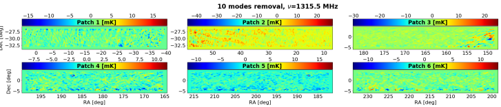
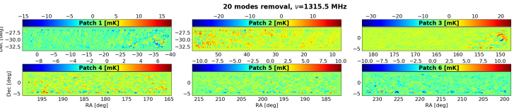
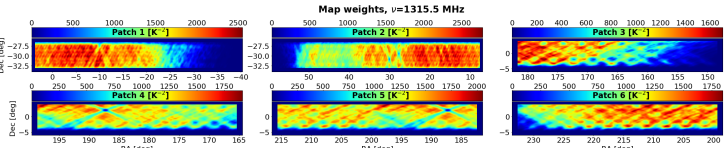
Figure 1: An example of the Parkes data used in this work. Top panel. 10-mode foreground removed 21-cm intensity maps shown in units of mK for all six patches in the (RA, Dec) frame for a single frequency/redshift slice, corresponding to the centre of the Parkes Multibeam Receiver bandwidth. Middle panel. Same as above, but showing the 20-mode foreground removed maps. Bottom panel. Plot of the map weights per patch in units $\text{K}^{-2}$ for the same frequency slice shown in the upper panels. Features clearly visible in these plots include the masking of local bright radio sources and the crossing of differently oriented stripes corresponding to the raster scanning of the telescope at constant elevation.

The present work aims at contributing to the search for neutral hydrogen in the local Universe, focussing this time on the 21-cm line from the spin-flip hyperfine transition in the hydrogen ground state (Pritchard & Loeb, 2012). Compared to the Lyman-$\alpha$ line, which for low redshift sources falls in the UV range and is therefore blocked by the atmosphere, the 21-cm emission lies in the microwave range which enables its detection using ground-based facilities. Pen et al. (2009) first showed the feasibility of tracing cosmic structures using 21-cm maps. Subsequent works relied on the cross-correlation between 21-cm and galaxy maps spectra to obtain estimates of the HI energy density parameter (Chang et al., 2010; Masui et al., 2013), agreeing in the estimate $\Omega_{\rm HI}\sim 6\times 10^{-4}$ at $z\sim 0.8$. The correlation between galaxies and HI at very low redshfit was also investigated in Anderson et al. (2018, hereafter A18). This approach for estimating the HI mass density relies on the expected full correlation between HI fluctutations and galaxy overdensities on large scales. The present study, conversely, targets specifically the cosmic web filaments, and aims at searching for the 21-cm signature from the neutral gas fraction in the WHIM. The feasibility of a direct detection of 21-cm emission from the filamentary gas has been explored in Kooistra et al. (2017). In this work, however, we adopt a methodology very similar to the one used by T19 and DG19, based on the stacking of galaxy pairs to enhance the signal coming from the large-scale filaments, and we employ the same data set used by A18, namely the 21-cm maps from the Parkes telescope and the galaxy catalogue from the Two-Degree-Field (2dF) survey. The final goal is to assess the amount of HI found in filaments at very low redshift ($z<0.1$), by providing estimates (or upper limits) on the HI column density $N_{\rm HI}$ and on the locally defined HI density parameter $\Omega_{\text{HI}}^{\rm(f)}$ (the superscript “f” is used to stress that this quantity is evaluated in filaments, and to distinguish it from the global HI density parameter in the Universe $\Omega_{\text{HI}}$). Such a result is complementary to the estimates based on the detection of the 21-cm emission proceeding from the HI confined inside galaxies, and shows the relative amount of neutral baryons that are to be found as a diffuse component in the cosmic web.

The paper is organised as follows. In Section 2 we describe the data set we employed and the pre-processing that was required by the subsequent analysis. The procedure for the extraction of the filamentary 21-cm signal and the determination of its uncertainty is detailed in Section 3. In Section 4 we discuss the significance of the results obtained from the galaxy-pair stacking. Section 5 is dedicated to the relation between the derived filament temperature and the corresponding local HI content. Finally, Section 6 presents the conclusions. Whenever the computation of cosmological quantities is required, throughout this work we adopt a flat $\Lambda$CDM cosmology with $\Omega_{\rm m}=0.3$, $\Omega_{\rm b}=0.049$, $\Omega_{\Lambda}=0.7$ and $H_{0}=70\,\text{km}\,\text{s}^{-1}\text{Mpc}^{-1}$.

2 Data set

We describe in this section the data set employed for our analysis. In order to detect the HI emission from intergalactic filaments we need a galaxy catalogue to identify the position and orientation of the filaments, and a sufficiently extended sky map in 21-cm to extract the corresponding signal. Clearly, the map and the catalogue must have a significant overlap in both angular and redshift coverage. We concluded that, in terms of the total covered sky area, the best choice that suits our purpose is a set of 21-cm maps obtained with the Parkes telescope with tailored observations that covered the region spanned by the 2dF Galaxy Catalogue. We describe both the maps and the catalogue in details in the following.

2.1 21-cm maps

We employ the 21-cm intensity maps from the Parkes Observatory described in A18. The starting point for our work are the foreground-cleaned maps, which can be considered to be representative of the HI emission alone. We redirect to the aforementioned reference for a detailed description of the full data processing involved in the production of the maps, including observational strategy, bandpass calibration, mapmaking algorithm and foreground removal. We limit this section to a description of the final product which is relevant for the subsequent analysis.

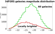
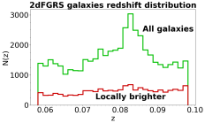
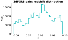
Figure 2: Left panel. Effect of the selection of locally brighter galaxies on the original 2dFGRS catalogue included in the Parkes data volume, in terms of the catalogue distribution in absolute R-band magnitude. Central panel. Same as in the left panel but showing the galaxy redshift distribution. Right panel. Redshift distribution for the final pair catalogue used in this work.

Data employed for the map-making came from a set of observations taken using the Parkes 21-cm Multibeam Receiver (Staveley-Smith et al., 1996) during a single week between April and May 2014, for a total observing time of 152 hours. The full Multibeam Correlator was employed with 1024 frequency channels over a full bandwith of 64 MHz centred at 1315.5 GHz, resulting in a 62.5 kHz frequency resolution. The Parkes beam sets the angular resolution at 14 arcmin. These observations aimed at covering the area spanned by the 2dF Galaxy Catalogue: the resulting maps cover two stripes, one in the northern and one in the southern Galactic hemisphere, resulting in a total sky coverage of $\sim 1,300$ square degrees. In order to improve the computational efficiency of the mapmaking code, these two main fields had been further divided into a total of six sub-fields, two in the southern and four in the northern Galactic hemisphere. Hereafter we shall label as “1” and “2” the southern patches, and from “3” to “6” the northern patches (see Fig. 1). Each patch was delivered in the form of a standard three-dimensional matrix: the three axes correspond to the J2000.0 equatorial coordinates and to frequency, (RA, Dec, $\nu$). The angular pixel size is 0.08 deg, while the frequency resolution was degraded to 1 MHz after local radio frequency interference removal. The resulting sampling in terms of pixel numbers is (486, 106, 64), which is common to all patches. Information about the spatial and frequency coverage for each patch, together with the corresponding pixel resolution, can be found in Table 1 (notice that the frequency range was the same for all the patches, being determined by the receiver configuration chosen for this set of observations).

At these frequencies the radio foregrounds, mainly Galactic and extra-Galactic synchrotron emission, are two to three orders of magnitude brighter than the 21-cm emission. As mentioned, these maps are already foreground-cleaned; the identification and removal of these foregrounds at the map level is described in A18 and is based on the algorithm detailed in Switzer et al. (2015). Given the dominant amplitude of the foregrounds, and their expected frequency smoothness compared to the 21-cm signal (Liu & Tegmark, 2012), the cleaning is based on a Principal Component Analysis (PCA) in which the higher frequency correlated modes are removed. The result will depend on the choice of the number of modes to be removed, taking into account that although each of these modes is dominated by foregrounds, it also carries a contribution from the 21-cm signal; consequently, the removal of a high number of modes yields cleaner maps but also implies a higher loss of HI signal. In A18 the 10-mode removed maps are used, and we will adopt the same choice for the present work. However, in order to assess the effect of the local residual foregrounds on our final estimates, we will also conduct the same analysis independently on the 20-mode removed maps.

In the top and middle panels of Fig. 1 we show the six patches 21-cm maps sliced at the central frequency of the Multibeam Receiver, for the cases of 10 and 20 foreground removal modes. The maps show both positive and negative structures at the $10\,\text{mK}$ level. It is clear from the right-ascension ranges that the northern patches are partially overlapping; however, each patch undergone independent foreground removal, and as a result the structure pattern is not the same comparing two different patches in their overlapping region, the difference being again of the order of a few mK. For this reason, in this work we will analyse each patch independently, which will allow us to establish the consistency of our results across the different Parkes fields. Additionally, we will present the results obtained by combining all the patches together, as the case with the highest statistical significance.

Apart from these 21-cm maps we were also provided with an analogous set of weight maps, which account for the non-homogeneous coverage of the observed fields. The weight maps are also split into six patches and are issued in the same resolution and pixelisation as the signal maps. The value stored in each pixel is the corresponding inverse squared noise weight, which is roughly proportional to the time spent observing it. The bottom panel of Fig. 1 shows the weight maps for a single frequency slice; the plot allows to recognise different structures, like the masking of local bright radio sources, appearing as dark spots, and the observation strategy, which produces bright stripes with different orientations. Indeed, data were acquired using azimuth scans at constant elevation, and the stripe orientation depends on the apparent motion of the field (rising or setting) during each observation. The highly spatial inhomogeneous amplitude of the weight maps is to be taken into account when combining the 21-cm intensities extracted from different regions of the signal maps.

2.2 Galaxy and pair catalogues

The Two-Degree-Field Galaxy Redshift Survey (2dFGRS, Colless et al., 2001) is a spectroscopic survey conducted between 1997 and 2002 using the 3.9 meter telescope at the Anglo-Australian Observatory; its data were released in June 2003. The survey provides spectroscopic redshifts for 245,591 sources distributed over two fields, one in the northern and one in the southern Galactic hemisphere, plus a set of additional random pointings scattered around the southern field. We downloaded the 2dFGRS “Catalogue of best spectroscopic observations” from the official website and performed a set of queries to extract the sources most suitable to our analysis.

We perform a first selection by considering only the sources with a reliable redshift determination, quantified by a quality parameter $q$ ranging from 1 to 5 (according to the 2dF documentation, only the sources with $q\geq 3$ can be considered reliable); we also discard the sources with a negative redshift estimation. This lowers the total number of sources to 227,190. Secondly, the catalogue is queried to select only the galaxies located within the angular and redshift span of the Parkes patches described in Section 2.1. In order to avoid possible strong residual contaminations from the patch edges, we also discard sources located within a Dec limit of $1\,\text{deg}$ and a RA limit of $3\,\text{deg}$ from each patch boundaries (the difference between these two values comes from the patch extensions in RA being a factor $\sim 3$ larger than the extensions in Dec). We also discard galaxies with redshift within the lowest 10 MHz and the highest 4 MHz of the Parkes frequency range, which according to A18 are also affected by higher noise due to band-edge effects. At this point the initial 2dFGRS catalogue is split into a set of six sub-catalogues, one for each Parkes patch. For the case of the overlapping Parkes fields, galaxies belonging to two patches are included in both the corresponding sub-catalogues. Indeed, as already mentioned, the analysis for each patch is conducted independently, and this choice improves the available statistics; when combining estimations from different patches, the resultant multiplicity is accounted for by using a proper weighting, as it is detailed in Section 3.2. In total, the restriction to the patch areas reduces the catalogue to a total of 36,800 galaxies, which amounts to 48,340 objects if we count each galaxy with its multiplicity.

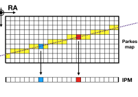
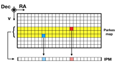
Figure 3: Extraction of an individual pair map (IPM) from the Parkes data cube, shown in this case in projection along the declination axis. The two pixels in red and blue host the galaxies forming the pair, while the pixels highlighted in yellow are the ones defining the IPM. Left. The method employed in this work is based on the projection along the frequency direction of the pixels intercepted by a plane parallel to the direction of the pair and to either the declination (as in this case) or the right-ascension axis, depending on the orientation of the pair in the three-dimensional data structure. This method assumes that the filament is aligned with the pair axis. Right. A more conservative average of the frequency/redshift slices spanned by the galaxy pair would have the effect of artificially lowering the intensity of any signal which is not extended across the slices.

The final query we perform on the catalogue aims at selecting the most likely tracers of the nodes in the cosmic web, which typically host massive galaxy clusters with early type galaxies. Ideally, one would consider the locally most massive objects, in order to focus on the central halo galaxies and discard the effect of satellite galaxies; however, the 2dFGRS catalogue does not provide the object masses. We therefore use the galaxy magnitude as a mass proxy, and consider the locally brighter galaxies in the R-band. We adopt an isolation criterion similar to the one proposed by Planck Collaboration et al. (2013) and also employed by T19: we discard a given galaxy if a brighter one is found within a tangential distance of $1.0\,h^{-1}\text{Mpc}$ and a line-of-sight (LoS) distance of $|c\Delta z|=1000\,\text{km}\,\text{s}^{-1}$. The online 2dFGRS catalogue provides the apparent R-band magnitude $m_{\text{R}}$ for each object, which for a redshift $z$ we convert into absolute magnitude using:

$$M_{\text{R}}=m_{\text{R}}-25-5\log_{10}{\left[\frac{D_{\text{L}}(z)}{\text{Mpc}}\right]},$$ (1)

where $D_{\text{L}}(z)$ is the luminosity distance at redshift $z$. The effect of this selection on the magnitude and redshift distribution of the galaxies is shown in the first two panels of Fig. 2. Apart from the overall reduction in the sample size, this cut tends to favour the brighter galaxies, which as expected become relatively more abundant, while keeping the redshift distribution roughly flat. The total number of selected galaxies is finally 13,979; the effective number per patch is reported in Table 1.

These catalogues are used to find the pairs of galaxies which are likely to host a filament in between. The pair selection adopts a criterion similar to the ones used by T19 and DG19: two galaxies are considered to form a valid pair if their tangential separation is in between 6 and 14$\,h^{-1}\text{Mpc}$, and their LoS separation is less than $6\,h^{-1}\text{Mpc}$. The resulting pair numbers per patch are reported in Table 1; overall, the selection yields 274,712 pairs, a number which is comparable to the sample size used by T19. The resulting redshift distribution for these pairs is shown in the third panel of Fig. 2.

3 Methodology for galaxy-pair stacking

The galaxies in the 2dFGRS pair catalogue described in Section 2.2 represent the endpoints of possible filaments in the LSS; in order for the signal coming from the neutral hydrogen component in these filaments to be measurable, their emission is to be combined in such a way as to enhance the the local filament signal with respect to the background. This is achieved via a proper pair stacking which resembles the works of DG19 and T19. The current analysis, however, presents a major difference: while their stacking was performed on the Compton parameter map, which has no depth, in our case the Parkes patches are also extended in the frequency/redshift direction. Our stacking algorithm requires therefore a prior step to extract a two-dimensional map for each individual pair; these maps can then be properly stacked together. Once the final stack maps are obtained, the signal coming from the galaxies defining the filament edges has to be removed, and from the resulting residual map it is possible to extract the filament signal. The evaluation of the uncertainties on the final filament emission is performed by repeating the stacking on a set of randomised maps and catalogues. We detail each one of these steps in the following.

3.1 Individual pair maps

A general valid galaxy pair is extended along all the three axes of right ascension, declination and frequency in the Parkes data cube; the first step consists in obtaining a map in two dimensions only, (RA, Dec), which carries the contribution of the pair: hereafter we will call such a map an “individual pair map” (IPM). For each pair two IPMs have to be evaluated, one for the HI signal and one for the corresponding weights.

The method we use is based on the projection of the pixel values along the line of sight (see Fig. 3, left panel, for a graphic representation). Let us consider a galaxy pair with ($\text{RA}_{1}$,$\text{Dec}_{1}$,$\nu_{1}$) and ($\text{RA}_{2}$,$\text{Dec}_{2}$,$\nu_{2}$) the coordinates of the two member galaxies; we label $\Delta\text{RA}$ and $\Delta\text{Dec}$ the absolute values of the separation along the two equatorial coordinates. We build the IPM by setting a pixel in the position (RA,Dec) to the value found in the pixel (RA,Dec,$\nu_{\rm proj}$) in the Parkes data cube, with the projection frequency $\nu_{\text{proj}}$ defined as:

$$\nu_{\text{proj}}(\xi)=\nu_{1}+\dfrac{\nu_{2}-\nu_{1}}{\xi_{2}-\xi_{1}}(\xi-\xi_{1}).$$ (2)

where the generic variable $\xi$ stands for either RA or Dec. If $\Delta\text{RA}\geq\Delta\text{Dec}$, then $\xi=\text{RA}$ and the value of $\nu_{\text{proj}}$ is the same for all the pixels in the IPM with the same right ascension; conversely, if $\Delta\text{RA}<\Delta\text{Dec}$, then $\xi=\text{Dec}$ and the value of $\nu_{\text{proj}}$ is the same for all the pixels in the IPM with the same declination. In other words, the IPM is built by projecting along the frequency direction a tilted plane defined by the separation vector and either the declination or the right ascension versor, depending on whether the galaxies are separated mostly in RA or Dec. By construction, this method preserves the values of the HI signal stored in the initial map; in particular, it provides an IPM which reports the correct amplitude for all the pixels on the line that joins the two galaxies in the Parkes data cube. For pairs located near the edges of the frequency band it is possible that for values of RA or Dec far from the pair centre the resulting value of $\nu_{\text{proj}}$ falls out of the allowed frequency range; in this case the affected IPM pixels are properly flagged and their values in the weight IPM is set to zero.

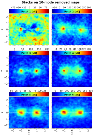
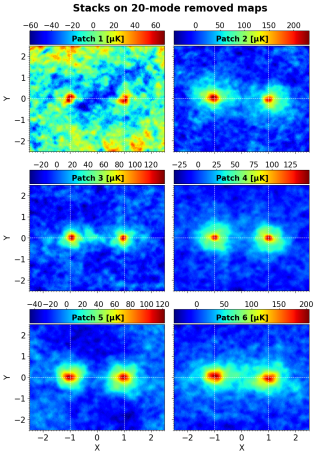
Figure 4: Final maps obtained by stacking the selected 2dFGRS galaxy pairs on the Parkes 21-cm maps, for the case of 10 (left) and 20 (right) modes removal. We show the results for all six patches; in order to enhance the details of these maps we chose to saturate the color scale for each patch, resulting in different ranges. With the exception of patch 1, which is apparently noisier, the rest of the stacks show similar patterns. The two peaks corresponding to the stacked 2dFGRS galaxies are clearly visible in their expected positions, but at this level the possible presence of a linking filament is not clear.

The method we have described implicitly assumes that the filaments connecting the galaxy pairs are straight lines. Any strong curvature of the filament would make it deviate from the segment joining the two endpoints and bring it out of the projection plane, meaning that it would not enter the corresponding IPM. We also explored a different method to work around this issue, based on the average of the contribution from all the frequency slices located in between the two galaxies (Fig. 3, right panel). This method allows to mitigate the loss of bent filaments, provided their curvature is not so large that it takes them outside the frequency range bounded by the two galaxies. However, this approach produces an artificial dilution of any signal that is not coherently repeated across slices along the line of sight (including the filament signal we are looking for), the effect being higher for larger redshift separations of the two galaxies. Given the complex spatial behaviour of both the signal and the weights in the three-dimensional Parkes patches, it is not possible to quantify the effect with a simple scaling factor to be applied in the end as a correction. Furthermore, we should notice that features that extend along the frequency direction and are enhanced by this method are usually foreground residuals, so the final IPM is likely to be affected by a higher foreground contamination.

For this work we decided to use the projection method for building the IPMs. Indeed, even though some filaments may lie outside the geometrical line joining their endpoints, the majority of the pair galaxies are separated by only one or two slices: while this is enough to dilute any filament signal by a factor 2 or 3 using the averaging method, it is unlikely that the filament spine avoids the totality of the pixels intercepted by the projection plane. In addition, the frequency resolution of the Parkes maps translates into a slice thickness of $\sim 2\,\text{Mpc}$, which is the typical expected diameter for a filament: although in some sections of the projection plane the filament spine may lie in the frequency slice right next to the one that is being considered, the filament outskirts are expected to enter the IPM in the projection. In any case, this is an approximation that undoubtedly affects the results of a filament blind search like the one we are undertaking in this work, and has to be acknowledged.

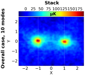
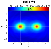
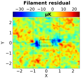
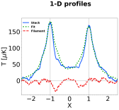
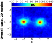
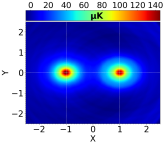
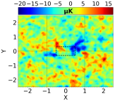
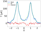
Figure 5: Results for the analysis of the full map obtained by combining the contribution of all patches (see eq. (5) in the text), shown for both the 10-mode (Top row) and the 20-mode (bottom row) removed maps. First column. Overall stacking result map; the improvement of the statistics deriving from combining the individual patch contributions determines a more homogeneous background in this final stack. Second column. The corresponding halo fit map, carrying the contribution from the galactic HI peaks only. Third column. The filament residual map, obtained by subtracting the halo-fit map from the stack map. Fourth column. The one dimensional profiles at Y=0 for the total stack, the halo fit and the filament residuals, confirming the absence of a net filament excess in the central region.

3.2 Stacking procedure

The galaxy pairs we consider have different positions, angular separations and orientations in the IPM maps. In order to make sure that the signal from the pair galaxies and the filament in between is added consistently, we have to bring all pairs to a common orientation. To this aim, we define a new reference frame (X,Y), with origin in the pair central coordinates and whose axes are defined in such a way that one of the galaxies lies in the position $(-1,0)$ and the other in the position $(+1,0)$. Each IPM is therefore brought to this common reference frame, by applying a rotation around the pair centre that brings the galaxies along the X-axis, and by rescaling the lengths by a common scale factor in order to place the galaxies at unit distance from the centre. This procedure is applied to both the signal and the weight IPMs, generating a set of final maps $S_{\text{XY}}^{i}$ and $W_{\text{XY}}^{i}$ for $i=1,...,N_{\rm p}$, with $N_{\rm p}$ the total number of pairs. The final stacked map for a given patch $n$ is then obtained as:

$$S_{n}=W_{n}^{-1}\,\sum_{i=1}^{N_{\text{p},n}}S_{\text{XY}}^{i}W_{\text{XY}}^{i},$$ (3)

where $N_{\text{p},n}$ is the total number of pairs for the patch and

$$W_{n}=\sum_{i=1}^{N_{\text{p},n}}W_{\text{XY}}^{i}$$ (4)

is the corresponding total weight. The resulting stack maps for the individual patches are shown in Fig. 4. We also consider the total stack map $S_{\rm T}$ obtained combining the results from individual patches. This is done again via a weighted average:

$$S_{\text{T}}=\dfrac{\sum_{n=1}^{6}S_{n}W_{n}}{\sum_{n=1}^{6}W_{n}}.$$ (5)

The result is shown in the leftmost panels of Fig. 5; hereafter we shall refer to this case as the overall stack.

3.3 Filament extraction

The final stack maps clearly show two peaks located in the expected positions $(\text{X},\text{Y})=(\pm 1,0)$. This emission proceeds from the HI bulk located inside the galaxies that we are stacking; since in our data set these galaxies have been selected to locate the LSS halos, we can refer to each of these peaks as the one-halo emission. This emission is clearly the dominant feature in our stacks, and any filament signal will be a second order contribution. In order to assess quantitatively the presence of actual filaments in the maps we have to remove the emission from the pair galaxies.

First of all, since we are interested in the relative emission excess with respect to the background, we evaluate the mean background level as the average of the pixels found in the external frame defined by the conditions $|\text{X}|>2$ or $|\text{Y}|>1.5$, and subtract it from each map as an overall offset. Secondly, for each stack we build a map carrying only the contribution from the halo peaks, obtained by fitting a halo profile on the stack maps. Notice that in this case it is not meaningful to derive an analytical expression to fit for; indeed, the one-halo profiles visible in the stacks are obtained from the superposition of several profiles from individual galaxies with different masses, each of which underwent a different rescaling during the processing of the corresponding IPM (depending on the initial pair separation in the (RA,Dec) frame, the profiles are either shrinked or stretched in order to match the final separation of $\Delta$X=$2$ in the (X,Y) frame). This implies that an analytical expression for the radial dependence of the HI intensity in these maps will be uncorrelated from the physical parameters describing the stacked halos (like their mass, brightness temperature or redshift).

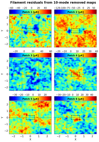
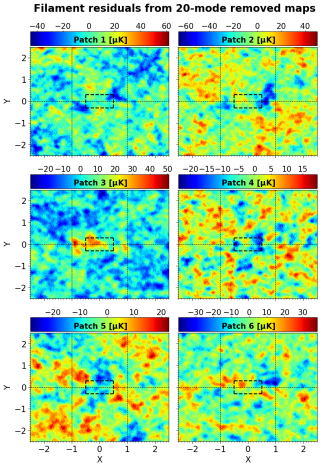
Figure 6: Filament residual maps for the six patches, obtained by subtracting from the stack maps in Fig. 4 the corresponding fitted halo profiles. Again, the scale is saturated for each individual patch in order to better show the background structures.

We therefore use a different approach and extract the profiles directly from the map, with the only assumption that the profile for each halo has to be circularly symmetric. For the peak centred in X=-1 we define a set of $N_{\rm b}$ bins $r_{i}$ (with $i=1,...,N_{\rm b}$) for the radial distance from the point $(-1,0)$ with separation $\Delta r=0.02$ in the scaled units; for a generic profile $P_{i}$ defined over these bins we can build a one-peak map $M_{-1}$ by assigning the value $P_{i}$ to all pixels with distance from the position $(-1,0)$ in the range $[r_{i},r_{i}+\Delta r]$. We can repeat the same procedure for the other peak centred in $(+1,0)$ and for a chosen profile $P_{j}$ we can build the corresponding map $M_{+1}$. The sum of the two one-peak maps, $M_{\text{peaks}}=M_{-1}+M_{+1}$, is our ansatz representing the halo-only contribution to the stack map. The final, best fit estimate of such a map is obtained by varying the one-halo profiles $P_{i}$ and $P_{j}$, and looking for the set of values that minimises the squared difference between the stack map and the peaks map. Since the maps are not perfectly symmetric, we allow the two halo peaks to have different radial profiles; plus, by fitting the sum of the two one-halo peak maps we also take into account the contribution of each galaxy profile on the other. In order for the final profiles to be representative of the halo contribution only, we restrict our fit to the external region of the map, in a frame defined by the conditions $|\text{X}|>1$ or $|\text{Y}|>1$. This way we ensure that the profile fit is not affected by any spurious filament contribution. An example of the resulting fit map, for the case of the overall stack, is shown in the second column panels of Fig. 5 (the fit maps for the individual patch cases are qualitatively very similar to these ones and do not provide any further information).

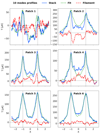
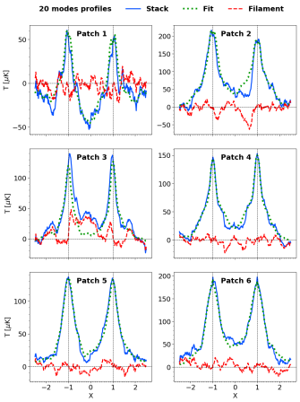
Figure 7: One dimensional cuts at Y=0 of the stacked maps from Fig. 4, the residual maps from Fig. 6 and the associated fit maps (not shown), for both the 10-mode (left) and the 20-mode (right) removal cases. Generally, the sum of the two individual profiles is enough to account for the signal visible in the central area, leaving no room for a filament contribution.

At this point, the subtraction between the stack map and the fitted halo map will be free from the galaxy contribution and show any possible filament emission in terms of an excess of signal in the central region. Fig. 6 shows the resulting filament residual map for each patch, while the third column panels in Fig. 5 show the filament maps for the overall stacks. The relative contributions from the stack and the fit are better visualised in terms of one-dimensional cuts of these maps; the corresponding profiles as a function of X at Y=0 (that is, along the galaxy pair axis), together with the residual filament contribution, are shown in Fig. 7 for the individual patches and in the fourth column panels of Fig. 5 for the overall stacks. However, the measurement of the filament emission is not performed on these cuts, but on the two-dimensional residual maps. The filament emission intensity is estimated as the mean of the map pixels found in the region $|\text{X}|<0.5$, $|\text{Y}|<0.3$, which is shown as a dashed box in the residual maps; the resulting values are plotted in Fig. 11 and will be discussed in Section 4.

3.4 Error estimation

In order to establish the significance for the filament detections we estimate their uncertainties adopting a bootstrap approach, based on the repetition of the stacking using a randomised data set. We consider two different implementations of this method.

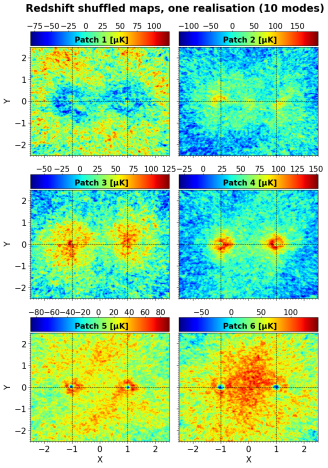
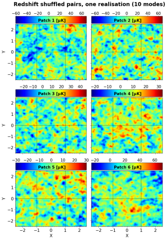
Figure 8: Results per patch of the two implementation of the bootstrap randomisation, shown for one particular realisation out of the total 500 for the 10-mode removed maps. Left. Stacking of the original pair catalogue on the Parkes maps with shuffled redshift slices. Right. Stack of the pair catalogue with shuffled redshifts on the original Parkes maps.

In the first case, we keep the pair catalogue unchanged and randomise the Parkes maps. The randomisation of individual pixel positions in the (RA, Dec) frame would not be appropriate because it would disrupt the correlation between adjacent pixels introduced by the Parkes beam, and create artificial structures with typical extension below the size of the main beam. We therefore shuffle the map redshifts: each frequency/redshift slice map is kept unchanged, but assigned to a different slice position, generated randomly; it is imposed that no slice can end up in its initial position after this shuffling, ensuring that all slices actually change their place. The same, new slice ordering is applied to all the six Parkes patches. We generate this way a set of 500 randomised Parkes maps, and for each one of them we repeat the same stacking procedure and filament extraction described for the case of the real data.

The second way we implement the bootstrap method is by keeping the maps unchanged and by randomising the pair catalogue. Again, we keep the (RA, Dec) coordinates of all pair galaxies fixed and only randomise their redshifts. Only the average redshift of each pair is changed, but not the redshift separation of the two member galaxies; the new average pair redshift is generated as a random number uniformly distributed in the range allowed by the Parkes maps. We generate this way 500 shuffled pair catalogues, each of which is stacked over the real Parkes data to obtain an estimation of the filament for each patch.

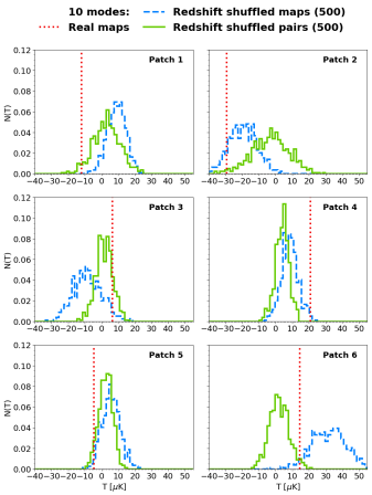
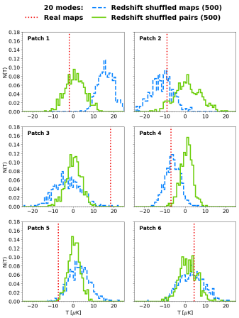
Figure 9: Significance of the filament detection shown for the six patches, for the 10-mode (left) and 20-mode (right) removal cases. The vertical line represents the detection on the real data, while the values obtained from the 500 random realisations are shown as histograms, one for each of the two methods. The distributions have been normalised to unit integral.

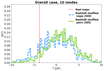
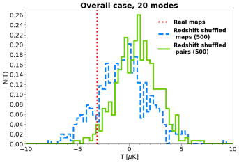
Figure 10: Same as in Fig. 9, but showing this time the detections and distributions on the overall maps obtained by combining the contributions from the six patches.

Fig. 8 shows the result of the stacking for both these two types of randomised data sets, in the case of one particular realisation. The result from both implementations of the bootstrap method is a set of 500 filament values for each patch and for the overall stack, shown respectively in Figs. 9 and 10 as histograms over the filament HI temperature. The dispersion of these values around their mean provides an estimate for the uncertainty of the filament detection in the corresponding patch case.

4 Discussion of stacking results

The initial stacks reported in Fig. 4 show that the contribution from the galactic HI emission is the dominant feature in the maps, and the region surrounding the galaxy pair looks quite uniform. The structures visible in patch 1 are at the same level as in the other patches, but the lower halo-peak amplitude in this case enhances their contrast. The overall stacks in Fig. 5 show the improvement in the quality of the stacking produced by the higher available statistics, which results in a more homogeneous background. However, although the signal pattern looks similar for all the stacks, its amplitude depends on the considered patch and on the foreground removal choice, with the 10-mode case being systematically higher; in general, there is no regular trend across the patches, or a clear relation between the number of pairs that are stacked and the differences in the final maps.

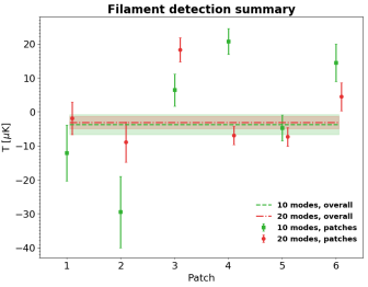
Figure 11: Summary of the filament detection analysis. The filament temperatures for all the patches are shown as points with their error-bars, for both the 10 and the 20-mode removed cases (the two sets points are shifted horizontally for displaying purposes). The estimates from the overall case that combines all patches are shown as horizontal dashed lines, and their uncertainties as a shaded region. Although the 20-mode removal case provides estimates closer to zero, the combination of all patches is compatible in the two cases.

At this level the presence of a filament bridging the two halo peaks is not clear, although some patches seem to show some overdensity in their centre, namely 3, 4 and 6 for the 10-mode case and 3 and 6 for the 20-mode case. Apart from this qualitative assessment it is still not clear whether the signal excess is coming from a diffuse source in the map centre or whether it is just produced by the superposition of the two decaying halo profiles.

The filament analysis described in Section 3.3 is devoted to clarifying this point. The second column panels in Fig. 5 show examples of the halo profiles we fit over the maps; our implementation is effective in reproducing the overall shape and amplitude of the profiles visible in the stacks. The fact that the fit is performed on the outermost region of the maps, and that the two halo profiles are fitted for at the same time, ensures a sensible assessment of the emission level in the map centre coming exclusively from the profile superposition. Any emission excess in this region must be due to additional sources that are located along the line connecting the halos, and would therefore prove the existence of a filament. The residual maps in Fig. 6 again point toward different conclusions depending on the considered patch. In the presence of an actual filament these maps would clearly show a positive residual in their centre, with a significative contrast with respect to the rest of the map. This is true only for patches number 4 and 6 in the 10-mode case, and for patch number 3 in the 20-mode case. All the other maps show a random distribution of positive and negative structures, without any emerging feature. Most importantly, the same can be said about the combination of all patches in the overall maps (Fig. 5, third column).

The one-dimensional cuts shown in Fig. 7 and in the last column panels of Fig. 5 provide further insights for understanding the features visible in the residual maps. Apart from the aforementioned patches showing a clear positive central residual, it is clear from these plots that negative features in the residual maps are produced by a local overestimation of the halo profiles. In many cases this is due to the profile being more extended in the external part of the maps, and falling more abruptly towards the centre. This effect basically proves the lack of a filament signal: although it is reasonable to assume that the halo profiles are circular symmetric, as we did for our fits, contributions from noise and possible foreground residuals will emerge in the final stacks as fluctuations over this symmetrical profile. When we subtract the halo signal, which is the dominant feature in the maps, these fluctuations will be enhanced. In the absence of a filament the final residual map signal will be at the level of the homogeneous background, and those fluctuations are expected to produce positive and negative structures, as observed in most of the stacks. In the case of a clear filament detection these fluctuations would still be second order compared to the filament signal: this is the case only for patches 4 and 6 in the 10-mode case, and for patch 3 in the 20-mode case. In all the other cases we can rule out the detection of a filament. There are other stacks with a positive central residual (patch 3 for the 10-mode case and patch 6 for the 20-mode case), but in those cases the local overdensity is comparable with the background fluctutations, hence they cannot be considered an evidence for a filament emission.

Regardless the appearance of the residual maps, we proceeded to the computation of the filament emission in the way described in Section 3.3 for all the stacks, and with the estimation of the corresponding uncertainties as detailed in Section 3.4. Fig. 8 shows a comparison between the two ways we implemented the randomisation of our data set, for one particular realisation. The stacking of the randomised catalogues produces final maps with no significant features: as expected, the halo peaks are no longer visible, and the distribution of fluctuations is homogeneous across the full area. The stack with the randomised maps, although lacking the clear peak signature that characterises the real data maps, still shows some residual structures in correspondence to the nominal galaxy positions, probably due to a combination of an insufficient randomisation of the slices and the non-homogeneous angular and redshift distribution of the galaxy pairs, which tend to favour local signal patterns. One other observation is that the typical size of the structures visible in the shuffled map stacks is smaller than the ones visible in the shuffled catalogue stacks, which are instead similar to the residual maps shown in Fig. 6 when we have no clear filament signature; this effect could be produced by the breaking of frequency coherent structures when shuffling the slices. The final width of the resulting distributions visible in Figs. 9 and 10 is comparable in the two cases, but the residual structures in the slice shuffling method determines a shift of the mean towards positive or negative values; the distributions obtained randomising the pair redshifts, instead, are more symmetrically centred at zero, as expected. For all these reasons we decided to discard the uncertainties estimated shuffling the maps and use only the ones obtained from the catalogue randomisation.

Fig. 11 summarises our filament detection for all individual patches and their combination, in the case of both 10 and 20-mode removal, together with the resulting uncertainties. The most evident feature emerging from this plot is the scatter of the values around zero, without any trend across different patches. Although there is some resemblance between the results obtained with different foreground removals, the two cases produce different estimates, with the 20-mode case being more consistently close to zero. The fact that the 10-mode removal case produces larger deviations from zero, both positive and negative, suggests that some foreground residuals may still affect the signal we are detecting. However, the random scatter across different patches indicates that these detections are probably dominated by noise; in these stack maps, the latter will be a combination of the initial map thermal noise and a number of systematic components deriving from our data processing (e.g. IPM extraction method, IPM rotation and scaling, choice of radial bins for the profile fitting, or region chosen for measuring the filament signal). When combining all the patches together, in any case, the filament temperatures estimated with different foreground removals are compatible; the resulting average is negative, which in the context of this stacking is non-physical. Although some patches, as already mentioned, produce a clear filament detection, we cannot consider only their contribution for the overall estimate, given that we have no a priori motivation for choosing some patches over others. Therefore, the conclusion of this analysis is that we do not detect a filament signal; this can be due either to the actual absence of HI in the filaments between the galaxy pairs we are considering, or to the fact that the noise level in the final filament maps masks the underlying HI emission.

In order to account for the latter case, we can quote upper limits on the HI temperature in the filaments; they are reported in Table 2, at the two-sigma level. Notice that for both the 10 and 20 mode cases the error for the overall stack, shown as a shaded region in Fig. 11, is lower than the standard error of the mean of the individual patch estimates. We decided to take a conservative approach and consider the mean standard error as representative of the final uncertainty associated with the filament signal in the overall stack. This uncertainty was used to compute the 95% confidence level upper limits; the combined estimate from the 10 and 20 mode cases points toward a local filament temperature of $T_{\rm b}\lesssim 7.5\,\mu\text{K}$ .

Table 2: Upper limits obtained for the filament HI brightness temperature, the locally defined cosmological HI density parameter, the local overdensity of neutral baryons and the HI column density. Values are reported for both the foreground removal cases, at $2\sigma$ confidence level.

	$T_{\rm b}$	$\Omega_{\rm HI}^{\rm(f)}$	$x_{\rm HI}\,\delta_{\rm b}$	$N_{\rm HI}$
	[$\mu\text{K}$]	$[10^{-5}]$	$[10^{-4}]$	$[10^{15}\,\text{cm}^{-2}]$
10 modes	$\lesssim$ 10.3	$\lesssim$ 7.0	$\lesssim$ 8.2	$\lesssim$ 4.6
20 modes	$\lesssim$ 4.8	$\lesssim$ 3.2	$\lesssim$ 3.8	$\lesssim$ 2.1

5 Estimation of HI abundance

In this section we use the estimates of the local filament excess temperature to infer upper limits on the HI abundance. The redshift distribution of the 2dFGRS catalogue, combined with the spatial separation constraints we imposed when defining a galaxy pair, results in a mean galactic angular separation of 2.8 degrees, which is considerably larger than the map resolution. Since this is the typical scale of the signal we want to detect, the dilution effect produced by the Parkes beam is negligible in this case, and the antenna temperature is equivalent to the local HI brightness temperature $T_{\rm b}$. For a given redshift $z$, the HI brightness temperature is related to the HI density parameter $\Omega_{\text{HI}}$ via (see for instance Hall et al., 2013):

$$\Omega_{\text{HI}}=7.6\times 10^{-3}\left[\dfrac{T_{\rm b}(z)}{\rm mK}\right]\,\left(\frac{h}{0.7}\right)^{-1}\left(1+z\right)^{-2}E(z),$$ (6)

where $E(z)=[\Omega_{\rm m}(1+z)^{3}+\Omega_{\Lambda}]^{1/2}$ is the ratio between the Hubble parameter at redshift $z$ and its present value. Our upper limits in the brightness temperature can thus be converted into upper limits on the hydrogen density parameter, which are reported in Table 2. Our evaluation suggests $\Omega_{\rm HI}^{\rm(f)}\lesssim 5\times 10^{-5}$, the upper limit being one order of magnitude lower than previous estimates of the HI abundance at low redshift. Observations in 21-cm of individual objects agree in $\Omega_{\rm HI}$ values in the range 3 to 5$\times 10^{-4}$, obtained by fitting for the HI mass function (Zwaan et al., 2005; Martin et al., 2010; Hoppmann et al., 2015) and by stacking galaxy spectra (Delhaize et al., 2013; Rhee et al., 2013). In our case, the low value of $\Omega_{\rm HI}^{\rm(f)}$ is due to the fact that it represents the local limit HI mass density inside a filament, but not the filament contribution to the total $\Omega_{\rm HI}$ in the Universe; the latter could be estimated if the total number of filaments and their size were known. In this context it is more meaningful to convert the brightness temperature into a measure of the local baryon overdensity $\delta_{\rm b}$; this can be constrained together with the neutral fraction of hydrogen $x_{\rm HI}$ using (Pritchard & Loeb, 2008):

$$\left(\dfrac{T_{\rm b}}{\mu\text{K}}\right)=\, 2.7\times 10^{4}\,x_{\rm HI}\left(1+\dfrac{4}{3}\delta_{\rm b}\right)\,\left(\dfrac{\Omega_{\rm b}h^{2}}{0.023}\right)$$

$$\times\left(\dfrac{0.15}{\Omega_{\rm m}h^{2}}\dfrac{1+z}{10}\right)^{1/2}\left(1-\dfrac{T_{\gamma}}{T_{\rm s}}\right),$$ (7)

where $T_{\gamma}$ is the CMB temperature and $T_{\rm s}$ the spin temperature. In our case, given the expected low density of HI in the intergalactic filaments, we are in the optically thin regime and $T_{\rm s}\gg T_{\gamma}$, which allows us to discard the last factor; we can also remove the unity term added to the baryon overdensity, because it represents the the mean HI contribution which is subtracted from our stacks. By substituting the values for our fiducial cosmology we obtain:

$$\left(\frac{x_{\rm HI}}{10^{-5}}\right)\left(\frac{\delta_{\rm b}}{10}\right)=0.80\,\left(\frac{T_{\rm b}}{\mu\text{K}}\right),$$ (8)

where the HI neutral fraction and baryon overdensity are normalised to the values typically expected in WHIM (see the discussion in Section 1). The substitution of our brightness temperature upper limits yields the estimates reported in Table 2 for the combination $x_{\rm HI}\,\delta_{\rm b}$. Since our overall temperature upper limit is $\sim 7.5\,\mu\text{K}$, the constraint imposed by eq. (8) is $x_{\rm HI}\,\delta_{\rm b}\lesssim 6\times 10^{-4}$, which is easily satisfied by the typical WHIM values for HI neutral fraction and baryon overdensity. In other words, our detection upper limits provide a loose constraint for the neutral baryon overdensity in filaments.

It is also useful in this context to estimate the HI column density, defined as the integral of the numerical HI density along the line of sight. In the optically thin regime the column density is related to the brightness temperature via (Meyer et al., 2017):

$$\left(\frac{N_{\rm HI}}{\text{cm}^{-2}}\right)=1.82\times 10^{15}\,\int\,\text{d}\left(\dfrac{\text{v}}{\text{km}\,\text{s}^{-1}}\right)\,\left[\frac{T_{\rm b}(\text{v})}{\text{mK}}\right],$$ (9)

where $T(\text{v})$ is the observed brightness at radial velocity $\text{v}=cz$, and the integral extends over the line profile. By using $1+z=\nu_{21}/\nu$, with $\nu_{21}$ the 21-cm line rest frequency and $\nu$ the observed frequency, the relation above can be recast as:

$$\left(\frac{N_{\rm HI}}{\text{cm}^{-2}}\right)=4.48\times 10^{14}\,\int\,\text{d}\left(\dfrac{\nu}{\text{MHz}}\right)\,\left[\frac{T_{\rm b}(\nu)}{\mu\text{K}}\right].$$ (10)

The integral can be approximated by the product of the integrand evaluated in the mean frequency of the maps, $\nu=1315.5\,\text{MHz}$, and the frequency channel width, $\Delta\nu=1\,\text{MHz}$; by inserting the measured upper limits in the HI brightness temperature, we obtain the estimates reported in Table 2, which average around $3.4\times 10^{15}\,\text{cm}^{-2}$. This value is significantly lower than the HI abundance found in halos; damped Ly $\alpha$ systems, for instance, generally have column densities $N_{\rm HI}>10^{22}\,\text{cm}^{-2}$ (Bird et al., 2017). Our estimate, however, is still about one order of magnitude higher than the HI content we would expect to observe in filaments, given that HI detections in WHIM have been performed at lower column densities (Richter et al., 2006; Nicastro et al., 2013). Again, although not representing a tight upper limit, our constraint is consistent with previous determination of the filament HI abundance.

The column density can also be evaluated using the estimates we obtained on the HI density parameter, provided the shape of the filaments is known. Assuming that the HI is uniformly distributed inside the filament, we can write:

$$N_{\rm HI}=\frac{\Omega_{\rm HI}^{\rm(f)}\rho_{c}}{m_{\rm HI}}(1+z)^{3}\,\Delta s,$$ (11)

where $m_{\rm HI}$ is the hydrogen atomic mass, $\rho_{c}$ is the Universe critical density and $\Delta s$ is filament extension along the line of sight. By substitution of the numerical values, and in astrophysical convenient units, the latter relation reads:

$$\left(\frac{N_{\rm HI}}{10^{15}\,\text{cm}^{-2}}\right)=0.21\left(\frac{\Omega_{\rm HI}^{\rm(f)}}{10^{-5}}\right)\left(\frac{\Delta s}{\text{Mpc}}\right).$$ (12)

In order to match the estimates in $\Omega_{\rm HI}^{\rm(f)}$ and $N_{\rm HI}$ reported in Table 2 the filament thickness is constrained to $\sim 3\,\text{Mpc}$. There is no universal definition for the typical filament radial extension; galaxies are usually considered filament members up to a radial distance of $0.5\,h^{-1}\text{Mpc}$ (Tempel et al., 2014) or $1\,h^{-1}\text{Mpc}$ (Kooistra et al., 2017) from the filament spine. The latter is consistent with our constraint if we take $\Delta s$ to represent the diametral filament size. This rough estimate serves as a consistency check of our estimated HI abundance.

5.1 Comparison with results from numerical simulations

To date there is no direct detection of neutral hydrogen in filaments from 21-cm observations; as mentioned in Section 1, most of the observational efforts have been devoted to the study of the ionised gas, while the detection of the neutral component relied on the observations of BLAs in the UV range. The detection of the HI 21-cm emission at the column density levels quoted in Table 2 is currently not feasible, and is the goal for the next generation of HI surveys. In this context, the use of numerical simulations becomes of paramount importance in order to provide hints on the conditions of the neutral gas in filaments; this information is also useful in assessing the best observational strategy to detect the faint filamentary HI signal. As far as the present work is concerned, results from simulations provide an interesting benchmark to compare our results.

We have already mentioned in the introduction that it is actually the study of cosmological hydrodynamical simulations that initially established the WHIM component as the most likely reservoir of missing baryons at low redshift. The first results from the seminal works by Cen & Ostriker (1999) and Davé et al. (1999) have been updated during the last two decades, following the improvements in the implementation of the baryon physics in the simulations, leading to the latest studies by Haider et al. (2016), Cui et al. (2019) and Martizzi et al. (2019). The latter work, in particular, was based on state-of-the-art numerical simulations that include a detailed characterisation of the baryonic physics involved in galaxy formation, evolution and feedback; the study explored the distribution of distinct baryonic phases, defined by cuts in the density-temperature phase diagram, across different structures of the cosmic web, namely nodes, filaments, sheets and voids. Qualitatively, the study reiterated the conclusion that the WHIM gas is mostly found at low redshift in filaments and nodes: at $z=0$ filaments account for the majority of the baryonic mass, where it is found as a combination of the WHIM and intergalactic medium (IGM) phases. The IGM in their work is identified as the gas component with density comparable to the WHIM, but with lower temperature ($T\lesssim 10^{5}\,\text{K}$). They also found that the IGM is rather ubiquitous across different cosmic structures, whereas the WHIM component is concentrated in the proximity of LSS filaments and nodes. The WHIM is therefore an effective tracer of the LSS filaments. Although the IGM component carries both ionised and neutral hydrogen, their work did not explicitly quote the final fraction of HI in filaments.

Studies with focus on the neutral baryonic component have also been tackled in the literature. In particular, Popping et al. (2009) showed how cosmological hydrodynamical simulations can conveniently complement real data below the current observational sensitivities. Starting from the output of a cosmological hydrodynamical simulation, they derived statistical properties for the hydrogen distribution which agree with observational constraints in the column density range for which data are available; this enables to study the simulated predictions below the observable limits. More precisely, they reconstructed the three-dimensional distribution of the total, neutral atomic and molecular hydrogen components, and extracted two dimensional maps for the corresponding column densities. The total hydrogen component clearly traces the typical cosmic web configuration and yields very high column densities in correspondence to the nodes, with peak values of $N_{\rm H}\sim 10^{21}\,\text{cm}^{-2}$, while the filaments are associated with values typically one order of magnitude lower. The $\text{H}_{2}$ column density map loses all the diffuse structures and exclusively retains the LSS nodes, which are the only locations where density and pressure are high enough to allow the formation of the molecular phase. This molecular gas generally hosts star formation, and the nodes correspond to massive galaxies and groups. The HI map also shows very high column densities in correspondence with the LSS nodes, but the signal is considerably lower for the filaments; nonetheless, the neutral atomic hydrogen still traces the large scale distribution of baryons, and in filaments the typical column density is $N_{\rm HI}\sim 10^{16}\,\text{cm}^{-2}$. This value is almost one order of magnitude higher than our upper limits from Table 2; we have to stress, however, that such an estimate is quoted in the aforementioned reference as a general value, but there is no clear explanation on how it has been obtained. From their map of the HI column density, filaments can clearly be identified at lower values of $N_{\rm HI}$, so their quote can be considered representative of the brightest filaments. More interestingly, they described a correlation between the HI column density and the expected neutral fraction of hydrogen $x_{\rm HI}$, with the gas being almost fully neutral at $N_{\rm HI}\gtrsim 10^{20}\,\text{cm}^{-2}$, but showing a steep increase in the ionised fraction as the column density decreases. When placing the values extracted from the simulation on a $x_{\rm HI}$–$N_{\rm HI}$ plane, the points scatter around a well defined curve; it is then meaningful to ask what is the most likely occurrence for the combination of neutral fraction and column density, as the region of the plot with the highest density of points. The conclusion is that $N_{\rm HI}\sim 10^{14}\,\text{cm}^{-2}$ and $x_{\rm HI}\sim 10^{-5}$ are the most commonly occurring conditions. At a column density of $N_{\rm HI}\sim 10^{15}\,\text{cm}^{-2}$, which is similar to our upper limit, their relation suggests a value for the neutral fraction just above $10^{-5}$, and, qualitatively, the probability of occurrence of this combined condition is still comparable to the maximum. Our upper limit on the combination $x_{\rm HI}\delta_{\rm b}$ is then consistent with this result if the filament overdensity is $\delta_{\rm b}\lesssim 60$. Since the local filament overdensities are typically in the range 10 to 100, our findings agree with the simulation results.

There have been subsequent studies focused on the prediction of properties of the neutral baryonic component based on numerical simulations (Duffy et al., 2012; Cunnama et al., 2014), although most of them do not target specifically the study of HI in filaments. The detectability of filamentary neutral gas using 21-cm observations has been investigated by Takeuchi et al. (2014). In that work the evolution of the abundance of different hydrogen ionisation states and the gas temperature in the IGM are at first computed analytically; the results enable the prediction of the typical HI brightness temperature and column density expected in filaments. Assuming a baryon overdensity of $\delta_{\rm b}=100$, the resulting column density for a filament which extends over $1\,h^{-1}\text{Mpc}$ along the line of sight is quoted to be $N_{\rm HI}\simeq 10^{15}-10^{16}\,\text{cm}^{-2}$, and assuming a proper LoS velocity of $\Delta\text{v}=300\,\text{km}\,\text{s}^{-1}$, the corresponding observed brightness temperature lies in the range $T_{\rm b}\simeq 10^{-6}-10^{-5}\,\text{K}$. Given the mean redshift and the bandwidth of the Parkes data we employed, in our case the mean LoS velocity is $\Delta\text{v}\simeq 245\,\text{km}\,\text{s}^{-1}$, implying a final brightness temperature a factor 1.2 lower; the results is still consistent with their estimates, and since their computed brightness temperature is proportional to the baryon overdensity and the filament LoS extension, we can easily accommodate a lower overdensity of $\delta_{\rm b}\sim 50$, consistent with the previous discussion about the neutral fraction, and a larger filament extension of $\sim 2.8\,\text{Mpc}$, comparable with our internal consistency check for the column density computed using the HI density parameter in filaments $\Omega_{\rm HI}^{\rm(f)}$. The study in Takeuchi et al. (2014) continues by comparing these estimates with the direct measurement of the filament properties on N-body simulations; they extracted the filament density contrast and LoS velocity from snapshots of the simulation at different redshits, and used them to estimate the brightness temperature; at $z=0$ they found that actually $\delta_{\rm b}\lesssim 100$, which yields a lower brightness temperature, at the $\mu\text{K}$ level. Again, this is in agreement with our upper limits.

The work by Horii et al. (2017) reprised this type of analysis, employing cosmological hydrodynamical simulations instead of N-body simulations; they stressed that the use of the latter would likely lead to an overestimation of the neutral fraction of gas in the filaments, due to the lack of feedback effects from galaxies. In any case, their results agree qualitatively with the previous ones, and show that HI is effective in tracing the filaments in the cosmic web; in the corresponding brightness temperature map at $z=0.5$, the signal shows peaks at the level of $10^{-4}\,\text{K}$ in the nodes, and lower values of $10^{-5}-10^{-6}\,\text{K}$ in the filaments. The comparison with the same map at $z=1$ shows that we can only expect a very mild decrease of these estimates to $z=0$, so that once again we find agreement with our upper limits. The work continues with the discussion on the possible contribution to the observed signal by filament galaxies, and provides an estimate for the brightness temperature coming from the diffuse WHIM component alone, resulting in even lower values of $\sim 10^{-8}\,\text{K}$ obtained by masking higher overdensity regions in the filaments. The detection of such a faint signal is clearly not feasible with any of the upcoming HI surveys, and will require the latest phases of the Square Kilometer Array (Braun et al., 2015); they also stated, however, that this result is affected by uncertainties regarding the actual contribution from filament galaxies.

Clearly, the detailed predictions from numerical simulations depend on the modelling of the physics underlying the formation and evolution of structures, and are also affected by the choice of the box size and resolution. Despite these drawbacks, they still represent a convenient gauge to test results like the ones presented in this study, in the absence of direct observational constraints. As far as our work is concerned, we find a general agreement between our upper limits and the simulated properties of HI at very low redshift. The continuous improvement in the modelling, resolution and size of numerical simulations can clearly provide a deeper understanding of the HI state in WHIM, although the ultimate confirmation can only be achieved with the next generation of 21-cm surveys.

6 Conclusions

This work attempts at finding HI emission from filaments connecting halos in the large-scale structure of matter in the Universe. In the framework of the missing baryon problem, the results of this analysis aim at constraining the amount of neutral hydrogen that can be found in the diffuse WHIM component. Previous work provided estimates based on BLA detection, but were limited to the study of a relatively small sample. This work addresses the analysis of the HI filament content by joining the contribution of a large number of objects distributed over an extended sky area ($\sim 1,300$ square degrees). It represents the analogous of the search for baryons that DG19 and T19 conducted on the Compton parameter map, but using for the first time the 21-cm signal of the HI component. It takes advantage of the capabilities of the low resolution HI intensity mapping technique of covering large areas on the sky, and resorts to a stacking procedure to enhance the signal that we are looking for.

We located the filament positions by selecting suitable pairs of 2dFGRS galaxies which define their endpoints, and measured the 21-cm signal on a set of Parkes maps produced by observations that spanned the 2dF survey area. For each individual pair we built a local two-dimensional 21-cm map by projecting a plane joining the two galaxies along the line of sight, and by rotating and scaling the local field of view in order to bring all the pairs to a common frame. We then co-added together these maps in order to enhance the filament contribution, and removed the HI signal proceeding from the pair galaxies by jointly fitting a pair of circular symmetric one-halo profiles on the final stacks. By joining the contribution of the six Parkes data patches, we stacked a total of 274,712 galaxy pairs with a mean redshift $z=0.079$. The final stacks clearly showed the contribution from the galactic HI emission, but once the fitted halo profiles were removed, the resulting residuals did not provide a clear evidence for a filament emission. Nonetheless, we estimated the local filament HI brightness temperature as the mean value of the residual maps in their central region, and assigned to each estimate an uncertainty determined as the variance of the residual signal from a set of 500 random realisation of the same analysis, obtained by stacking redhift shuffled versions of the galaxy pair catalogue.

The final values for the filament brightness temperature show a random dependence on the considered sky patch, with the results from the 20 foreground modes removed maps being more consistently close to zero than the 10-mode case. This suggests that a possible filament signal is at the same level of, or lower than, the noise fluctutations in the final maps, to which residual foregrounds may contribute to some extent; this conclusion is corroborated by the fact that many estimates are negative. The overall stack obtained combining all patches shows consistency across the two foreground removal cases, within the error bars generated with the bootstrap method. Since these errors are lower than the standard deviation of the mean computed from the individual patch detections, we considered the latter to be a more sensible estimate for the measured filament residual uncertainty. This allows us to set an overall upper limit for the filament HI brightness temperature at $T_{\rm b}\sim 7.5\,\mu\text{K}$, which is converted into a local filament HI cosmological density parameter as $\Omega_{\rm HI}^{\rm(f)}\sim 5\times 10^{-5}$ and column density as $N_{\rm HI}\sim 3.4\times 10^{15}\,\text{cm}^{-2}$. The value of $\Omega_{\rm HI}^{\rm(f)}$ is low compared to previous low-redshift estimates because it represents the local HI density parameter inside the filaments, but not the filament contribution to the global $\Omega_{\rm HI}$ in the Universe. The constraint on $N_{\rm HI}$ is one order of magnitude higher than the typical HI column density expected from observations of BLA absorbers in the UV range; although not representing a tight upper limit, it is consistent with previous HI detections in WHIM. The brightness temperature also allowed us to derive a joint constraint on the filament baryon overdensity and neutral fraction; again, the resulting upper limit easily accommodates the expected WHIM physical conditions. These results suggest that, if any actual HI component is present in the filaments we considered, its 21-cm emission lies at a level that cannot be detected with the set of maps employed in this work. Finally, we compared our estimates with results obtained from cosmological hydrodynamical simulations. Although the predicted properties of the low-redshift HI diffuse gas vary between different studies, simulations generally agree in showing how neutral hydrogen can effectively trace the cosmic web at $z=0$, and provide a useful benchmark in the absence of observational constraints; we found our upper limits to be in agreement with the simulated HI properties at $z\simeq 0$.

Notice that this paper analysis can easily be adapted to a different data set, provided extended 21-cm maps have a significant overlap with a chosen galaxy catalog. In particular, it would be interesting to conduct the same study at higher redshift, where the fraction of neutral gas is expected to be larger. Observations with the GBT telescope centred at $z\sim 0.8$ have been used in Chang et al. (2010) and Masui et al. (2013), in cross-correlation with optical surveys; however, the sky area explored in those works is considerably smaller than the one we employed. At very low redshift, future work can be addressed to tighten the upper limits on the HI filament content. The ALFALFA survey (Haynes et al., 2018) conducted with the Arecibo telescope provides HI detections at $z<0.06$; however, the legacy data consist of individual object catalogues, and not in continuous maps.

In conclusion, the search for HI in filaments using HI intensity mapping and stacking techniques requires extended maps in the 21-cm emission. Being able to analyse a large sky area is crucial in increasing the statistics of the galaxy pairs, and in enhancing a possible filament signal; besides, being able to explore different sky regions would lead to more sensible conclusions, mitigating the effects of local sample variance. Surveys conducted using next-generation facilities like the Square Kilometer Array (Braun et al., 2015) and the FAST telescope (Li & Pan, 2016) are expected to provide improved maps over a larger sky area thanks to the higher sensitivity and survey speed. A proper foreground removal clearly remains the critical point for delivering final maps with sufficient sensitivity to enable a detection of the filament HI signal.

References

- Alam et al. (2015) Alam S., et al., 2015, ApJS, 219, 12
- Anderson et al. (2018) Anderson C. J., et al., 2018, MNRAS, 476, 3382
- Bird et al. (2017) Bird S., Garnett R., Ho S., 2017, MNRAS, 466, 2111
- Braun et al. (2015) Braun R., Bourke T., Green J. A., Keane E., Wagg J., 2015, Advancing Astrophysics with the Square Kilometre Array (AASKA14), p. 174
- Bregman (2007) Bregman J. N., 2007, ARA&A, 45, 221
- Buote et al. (2009) Buote D. A., Zappacosta L., Fang T., Humphrey P. J., Gastaldello F., Tagliaferri G., 2009, ApJ, 695, 1351
- Cen & Ostriker (1999) Cen R., Ostriker J. P., 1999, ApJ, 514, 1
- Cen & Ostriker (2006) Cen R., Ostriker J. P., 2006, ApJ, 650, 560
- Chang et al. (2010) Chang T.-C., Pen U.-L., Bandura K., Peterson J. B., 2010, Nature, 466, 463
- Colless et al. (2001) Colless M., et al., 2001, MNRAS, 328, 1039
- Cooke & Fumagalli (2018) Cooke R. J., Fumagalli M., 2018, Nature Astronomy, 2, 957
- Cooke et al. (2018) Cooke R. J., Pettini M., Steidel C. C., 2018, ApJ, 855, 102
- Cui et al. (2019) Cui W., et al., 2019, MNRAS, 485, 2367
- Cunnama et al. (2014) Cunnama D., Andrianomena S., Cress C. M., Faltenbacher A., Gibson B. K., Theuns T., 2014, MNRAS, 438, 2530
- Danforth et al. (2010) Danforth C., Stocke J. T., Shull J., Savage B. D., Sembach K. R., 2010, in American Astronomical Society Meeting Abstracts #215. p. 502
- Davé et al. (1999) Davé R., Hernquist L., Katz N., Weinberg D. H., 1999, ApJ, 511, 521
- Davé et al. (2001) Davé R., et al., 2001, ApJ, 552, 473
- De Graaff et al. (2019) De Graaff A., Cai Y.-C., Heymans C., Peacock J. A., 2019, A&A, 624, A48
- Delhaize et al. (2013) Delhaize J., Meyer M. J., Staveley-Smith L., Boyle B. J., 2013, MNRAS, 433, 1398
- Duffy et al. (2012) Duffy A. R., Kay S. T., Battye R. A., Booth C. M., Dalla Vecchia C., Schaye J., 2012, MNRAS, 420, 2799
- Eckert et al. (2015) Eckert D., et al., 2015, Nature, 528, 105
- Fang et al. (2007) Fang T., Canizares C. R., Yao Y., 2007, ApJ, 670, 992
- Fields et al. (2014) Fields B. D., Molaro P., Sarkar S., 2014, arXiv e-prints,
- Fukugita & Peebles (2004) Fukugita M., Peebles P. J. E., 2004, ApJ, 616, 643
- Fukugita et al. (1998) Fukugita M., Hogan C. J., Peebles P. J. E., 1998, ApJ, 503, 518
- Génova-Santos et al. (2015) Génova-Santos R., Atrio-Barandela F., Kitaura F.-S., Mücket J. P., 2015, ApJ, 806, 113
- Haider et al. (2016) Haider M., Steinhauser D., Vogelsberger M., Genel S., Springel V., Torrey P., Hernquist L., 2016, MNRAS, 457, 3024
- Hall et al. (2013) Hall A., Bonvin C., Challinor A., 2013, Phys. Rev. D, 87, 064026
- Haynes et al. (2018) Haynes M. P., et al., 2018, ApJ, 861, 49
- Hernández-Monteagudo et al. (2015) Hernández-Monteagudo C., Ma Y.-Z., Kitaura F. S., Wang W., Génova-Santos R., Macías-Pérez J., Herranz D., 2015, Physical Review Letters, 115, 191301
- Hinshaw et al. (2013) Hinshaw G., et al., 2013, ApJS, 208, 19
- Hoppmann et al. (2015) Hoppmann L., Staveley-Smith L., Freudling W., Zwaan M. A., Minchin R. F., Calabretta M. R., 2015, MNRAS, 452, 3726
- Horii et al. (2017) Horii T., Asaba S., Hasegawa K., Tashiro H., 2017, PASJ, 69, 73
- Ibaraki et al. (2014) Ibaraki Y., Ota N., Akamatsu H., Zhang Y.-Y., Finoguenov A., 2014, A&A, 562, A11
- Kooistra et al. (2017) Kooistra R., Silva M. B., Zaroubi S., 2017, MNRAS, 468, 857
- Kull & Böhringer (1999) Kull A., Böhringer H., 1999, A&A, 341, 23
- Li & Pan (2016) Li D., Pan Z., 2016, Radio Science, 51, 1060
- Liu & Tegmark (2012) Liu A., Tegmark M., 2012, MNRAS, 419, 3491
- Ma et al. (2015) Ma Y.-Z., Van Waerbeke L., Hinshaw G., Hojjati A., Scott D., Zuntz J., 2015, J. Cosmology Astropart. Phys., 9, 046
- Martin et al. (2010) Martin A. M., Papastergis E., Giovanelli R., Haynes M. P., Springob C. M., Stierwalt S., 2010, ApJ, 723, 1359
- Martizzi et al. (2019) Martizzi D., et al., 2019, MNRAS, 486, 3766
- Masui et al. (2013) Masui K. W., et al., 2013, ApJ, 763, L20
- Meyer et al. (2017) Meyer M., Robotham A., Obreschkow D., Westmeier T., Duffy A. R., Staveley-Smith L., 2017, Publ. Astron. Soc. Australia, 34
- Nicastro et al. (2008) Nicastro F., Mathur S., Elvis M., 2008, Science, 319, 55
- Nicastro et al. (2013) Nicastro F., et al., 2013, ApJ, 769, 90
- Pen et al. (2009) Pen U.-L., Staveley-Smith L., Peterson J. B., Chang T.-C., 2009, MNRAS, 394, L6
- Persic & Salucci (1992) Persic M., Salucci P., 1992, MNRAS, 258, 14P
- Pessa et al. (2018) Pessa I., et al., 2018, MNRAS, 477, 2991
- Planck Collaboration et al. (2013) Planck Collaboration et al., 2013, A&A, 557, A52
- Planck Collaboration et al. (2016) Planck Collaboration et al., 2016, A&A, 594, A22
- Planck Collaboration et al. (2018) Planck Collaboration et al., 2018, arXiv e-prints, p. arXiv:1807.06209
- Popping et al. (2009) Popping A., Davé R., Braun R., Oppenheimer B. D., 2009, A&A, 504, 15
- Pritchard & Loeb (2008) Pritchard J. R., Loeb A., 2008, Phys. Rev. D, 78, 103511
- Pritchard & Loeb (2012) Pritchard J. R., Loeb A., 2012, Reports on Progress in Physics, 75, 086901
- Rauch (1998) Rauch M., 1998, ARA&A, 36, 267
- Rauch et al. (1997) Rauch M., et al., 1997, ApJ, 489, 7
- Rhee et al. (2013) Rhee J., Zwaan M. A., Briggs F. H., Chengalur J. N., Lah P., Oosterloo T., van der Hulst T., 2013, MNRAS, 435, 2693
- Richter et al. (2006) Richter P., Savage B. D., Sembach K. R., Tripp T. M., 2006, A&A, 445, 827
- Scharf et al. (2000) Scharf C., Donahue M., Voit G. M., Rosati P., Postman M., 2000, ApJ, 528, L73
- Shull et al. (2012) Shull J. M., Smith B. D., Danforth C. W., 2012, ApJ, 759, 23
- Staveley-Smith et al. (1996) Staveley-Smith L., et al., 1996, Publ. Astron. Soc. Australia, 13, 243
- Sutherland & Dopita (1993) Sutherland R. S., Dopita M. A., 1993, ApJS, 88, 253
- Switzer et al. (2015) Switzer E. R., Chang T.-C., Masui K. W., Pen U.-L., Voytek T. C., 2015, ApJ, 815, 51
- Takeuchi et al. (2014) Takeuchi Y., Zaroubi S., Sugiyama N., 2014, MNRAS, 444, 2236
- Tanimura et al. (2019) Tanimura H., et al., 2019, MNRAS, 483, 223
- Tempel et al. (2014) Tempel E., Kipper R., Saar E., Bussov M., Hektor A., Pelt J., 2014, A&A, 572, A8
- Ursino et al. (2014) Ursino E., Galeazzi M., Huffenberger K., 2014, ApJ, 789, 55
- Van Waerbeke et al. (2014) Van Waerbeke L., Hinshaw G., Murray N., 2014, Phys. Rev. D, 89, 023508
- Weinberg et al. (1997) Weinberg D. H., Miralda-Escudé J., Hernquist L., Katz N., 1997, ApJ, 490, 564
- Werner et al. (2008) Werner N., Finoguenov A., Kaastra J. S., Simionescu A., Dietrich J. P., Vink J., Böhringer H., 2008, A&A, 482, L29
- Zappacosta et al. (2002) Zappacosta L., Mannucci F., Maiolino R., Gilli R., Ferrara A., Finoguenov A., Nagar N. M., Axon D. J., 2002, A&A, 394, 7
- Zappacosta et al. (2010) Zappacosta L., Nicastro F., Maiolino R., Tagliaferri G., Buote D. A., Fang T., Humphrey P. J., Gastaldello F., 2010, ApJ, 717, 74
- Zwaan et al. (2005) Zwaan M. A., Meyer M. J., Staveley-Smith L., Webster R. L., 2005, MNRAS, 359, L30