Electron and photon performance measurements with the ATLAS detector using the 2015–2017 LHC proton–proton collision data \AtlasAbstract This paper describes the reconstruction of electrons and photons with the ATLAS detector, employed for measurements and searches exploiting the complete LHC Run 2 dataset. An improved energy clustering algorithm is introduced, and its implications for the measurement and identification of prompt electrons and photons are discussed in detail. Corrections and calibrations that affect performance, including energy calibration, identification and isolation efficiencies, and the measurement of the charge of reconstructed electron candidates are determined using up to 81 fb-1 of proton–proton collision data collected at TeV between 2015 and 2017. \AtlasRefCodeEGAM-2018-01 \AtlasJournalJINST \PreprintIdNumberCERN-EP-2019-145 \AtlasJournalRefJINST 14 (2019) P12006 \AtlasDOI10.1088/1748-0221/14/12/P12006 \AtlasCoverSupportingNoteSuper-cluster reconstructionhttps://cds.cern.ch/record/2298955 \AtlasCoverSupportingNoteElectron and photon energy calibrationhttps://cds.cern.ch/record/2651890 \AtlasCoverSupportingNoteElectron IDhttps://cds.cern.ch/record/2652163 \AtlasCoverSupportingNotePhoton IDhttps://cds.cern.ch/record/2647979 \AtlasCoverSupportingNoteElectron and photon isolationhttps://cds.cern.ch/record/2646265 \AtlasCoverCommentsDeadline10 July 2019 \AtlasCoverAnalysisTeamMaria Josefina Alconada Verzini, Francisco Alonso, Christos Anastopoulos, Nansi Andari, Ludovica Aperio Bella, Jean-Francois Arguin, Hicham Atmani, Cyril Becot, Maarten Boonekamp, Frued Braren, Kurt Brendlinger, Chav Chhiv Chau, Olympia Dartsi, Jean-Baptiste de Vivie de Régie, David Delgove, Lucia Di Ciaccio, David Di Valentino, Otilia Anamaria Ducu, Johannes Erdmann, Marc Escalier, Saskia Falke, Yi Fang, Marcello Fanti, Louis Fayard, Alexandra Fell, Lucas Macrorie Flores, Gregor Gessner, Dag Ingemar Gillberg, Dominique Godin, Thibault Guillemin, Sarah Heim, Rachel Hyneman, Lydia Iconomidou-Fayard, Oleh Kivernyk, Matthew Henry Klein, Thomas Koffas, Kevin Kroeninger, Joe Kroll, Antoine Laudrain, Yanwen Liu, Kristin Lohwasser, Stefano Manzoni, Julien Maurer, Jovan Mitrevski, Kazuya Mochizuki, Emmanuel Monnier, Miha Muskinja, Roger Felipe Naranjo Garcia, Isabel Nitsche, Ioannis Nomidis, Jose Ocariz, Andreas Petridis, Pavel Podberezko, Thomas Dennis Powell, Pascal Pralavorio, Nadezda Proklova, Joseph Reichert, Amartya Rej, Elias Michael Ruettinger, Abhishek Sharma, Nima Sherafati, Philip Sommer, Kerstin Tackmann, Grigore Tarna, Savannah Jennifer Thais, Evelyn Thomson, Artur Trofymov, Guillaume Unal, Hanlin Xu, Zhiqing Zhang \AtlasCoverEdBoardMemberOlivier Arnaez (chair) \AtlasCoverEdBoardMemberFares Djama \AtlasCoverEdBoardMemberKun Liu \AtlasCoverEgroupEditorsatlas-EGAM-2018-01-editors@cern.ch \AtlasCoverEgroupEdBoardatlas-EGAM-2018-01-editorial-board@cern.ch \LEcontactNorman Mccubbin, norman.mccubbin@stfc.ac.uk
Contents
\@afterheading\@starttoc
toc
1 Introduction
With an integrated luminosity of about 147 fb-1, the proton–proton () collision dataset collected by the ATLAS detector between 2015 and 2018 at a centre-of-mass energy of TeV will allow significant advances in the exploration of the electroweak scale. Optimal performance in the measurement of electrons and photons plays a fundamental role in searches for new particles, in the measurement of Standard Model cross-sections, and in the precise measurement of the properties of fundamental particles such as the Higgs and bosons and the top quark.
The ATLAS Collaboration published three papers describing the performance of the reconstruction, identification and energy measurement of electrons and photons with 36 fb-1 of collision data collected in 2015 and 2016 [1, 2, 3]. New algorithms for electron and photon reconstruction were introduced in 2017. The present paper describes the performance of these algorithms, and extends the analysis to the dataset collected between 2015 and 2017, which corresponds to an integrated luminosity of about 81 fb-1. The discussion is limited to electrons and photons reconstructed in the central calorimeters, covering the pseudorapidity range .
The transition from the reconstruction of electrons and photons based on fixed-size clusters of calorimeter cells towards a dynamical, topological cell clustering algorithm [4] represents the most important modification. The algorithms used for the identification of the candidates and the estimation of their energy have been updated accordingly. The performance of these changes is discussed in detail. In addition, methods allowing an improved rejection of misreconstructed or non-isolated candidates are presented, and are of particular importance for measurements of processes with low cross-sections or high backgrounds, such as the associated production of a Higgs boson with a top-quark pair, or vector-boson scattering at high energy.
After a summary of the experimental apparatus and the samples used for this analysis in Sections 2 and 3, Section 4 describes the new reconstruction of clusters of energy deposits in the electromagnetic (EM) calorimeter, the estimation of their energy, and the use of information from the inner tracking detector to distinguish between electrons and photons. Section 5 summarizes the energy calibration corrections and the associated systematic uncertainties. Sections 6 and 7 present the re-optimized electron and photon identification algorithms. Section 8 discusses the discrimination between prompt electrons and photons and backgrounds from hadron decays. Finally, studies dedicated to the electron and positron charge identification are reported in Section 9.
2 ATLAS detector
The ATLAS experiment [5, 6, 7] is a general-purpose particle physics detector with a forward–backward symmetric cylindrical geometry and almost 4 coverage in solid angle.111ATLAS uses a right-handed coordinate system with its origin at the nominal interaction point (IP) in the centre of the detector and the -axis along the beam pipe. The -axis points from the IP to the centre of the LHC ring, and the -axis points upward. Cylindrical coordinates are used in the transverse plane, being the azimuthal angle around the -axis. The pseudorapidity is defined in terms of the polar angle as . The angular distance is defined as . The transverse energy is . The inner tracking detector (ID) covers the pseudorapidity range and consists of a silicon pixel detector, a silicon microstrip detector (SCT), and a transition radiation tracker (TRT) in the range . The TRT provides electron identification capability through the detection of transition radiation photons. It consists of small-radius drift tubes (‘straws’) interleaved with a polymer material creating transition radiation for particles with a large Lorentz factor. This radiation is absorbed by the Xe-based gas mixture filling the straws, discriminating electrons from hadrons over a wide energy range. Due to gas leaks, some TRT modules are filled with an Ar-based gas mixture. The ID is surrounded by a superconducting solenoid producing a 2 T magnetic field and provides accurate reconstruction of tracks from the primary collision region. It also identifies tracks from secondary vertices, permitting an efficient reconstruction of photon conversions in the ID up to a radius of about 800 mm.
The EM calorimeter is a lead/liquid-argon (LAr) sampling calorimeter with an accordion geometry. It is divided into a barrel section (EMB) covering the pseudorapidity region ,222The EMB is split into two half-barrel modules, which cover the positive and negative regions. and two endcap sections (EMEC) covering . The barrel and endcap calorimeters are immersed in three LAr-filled cryostats, and are segmented into three layers for . The first layer, covering and , has a thickness of about 4.4 radiation lengths () and is finely segmented in the direction, typically in in the EMB, to provide an event-by-event discrimination between single-photon showers and overlapping showers from the decays of neutral hadrons. The second layer (L2), which collects most of the energy deposited in the calorimeter by photon and electron showers, has a thickness of about and a granularity of in . A third layer, which has a granularity of in and a depth of about 2, is used to correct for leakage beyond the EM calorimeter for high-energy showers. In front of the accordion calorimeter, a thin presampler layer (PS), covering the pseudorapidity interval , is used to correct for energy loss upstream of the calorimeter. The PS consists of an active LAr layer with a thickness of 1.1 cm (0.5 cm) in the barrel (endcap) and has a granularity of . The transition region between the EMB and the EMEC, , has a large amount of material in front of the first active calorimeter layer ranging from 5 to almost . This section is instrumented with scintillators located between the barrel and endcap cryostats, and extending up to .
The hadronic calorimeter, surrounding the EM calorimeter, consists of an iron/scintillator tile calorimeter in the range and two copper/LAr calorimeters spanning . The acceptance is extended by two copper/LAr and tungsten/LAr forward calorimeters extending up to 4.9, and hosted in the same cryostats as the EMEC. Electron reconstruction in the forward calorimeters is not discussed in this paper.
The muon spectrometer, located beyond the calorimeters, consists of three large air-core superconducting toroid systems with eight coils each, with precision tracking chambers providing accurate muon tracking for and fast-triggering detectors up to .
A two-level trigger system [8] is used to select events. The first-level trigger is implemented in hardware and uses a subset of the detector information to reduce the accepted rate to a maximum of about . This is followed by a software-based trigger that reduces the accepted event rate to on average, depending on the data-taking conditions.
3 Collision data and simulation samples
3.1 Dataset
The analyses described in this paper use the full collision dataset recorded by ATLAS between 2015 and 2017 with the LHC operating at a centre-of-mass energy of = 13 TeV and a bunch spacing of 25 ns. The dataset is divided into two subsamples according to the typical mean number of interactions per bunch crossing, , with which it was recorded :
-
•
The ‘low-’ sample was recorded in 2017 with ; after application of data-quality requirements, the integrated luminosity amounts to 147 pb-1.
-
•
The ‘high-’ sample corresponds to an integrated luminosity of 80.5 fb-1; for this sample, was on average 13, 25 and 38 for 2015, 2016 and 2017 data, respectively. The corresponding integrated luminosities are 3.2 fb-1, 33.0 fb-1 and 44.3 fb-1. In 2016, a small sample corresponding to 0.7 fb-1 of data was recorded without magnetic field in the muon system; it is added to the ‘high-’ sample for electron reconstruction and identification studies.
Two different LHC filling schemes were used in 2017. The nominal filling scheme, labelled 48b in the following, corresponding to an integrated luminosity of 17.9 fb-1 and , was built from ‘sub-trains’ of 48 filled bunches followed by seven empty bunches. Simulated event samples use this configuration,333The simulation used in conjunction with 2015 and 2016 data has a similar bunch configuration, consisting of 72 filled bunches followed by eight empty bunches. as it represents about 70% of the collected data; the implications of this approximation for the energy calibration are discussed in Section 5. The second scheme, labelled 8b4e, corresponding to an integrated luminosity of 26.4 fb-1 and , was made of sub-trains of eight filled bunches followed by four empty bunches. To sustain these conditions, a levelling of the instantaneous luminosity at cm-2s-1 was necessary at the beginning of the fill, resulting in a peak around 60. The noise induced by pile-up, or multiple interactions occurring in the same bunch crossing as the event of interest or in nearby crossings, is 10% smaller than for the standard configuration for a given . The LHC filling scheme for the ‘low-’ data sample was 8b4e.
Several levels of object identification and isolation criteria are employed to select the event samples used in the analyses described in this paper. Electrons are identified using a likelihood-based method combining information from the EM calorimeter and the ID. Different identification working points, Loose, Medium and Tight are defined [2]. Similar levels are used at trigger level (online), with slightly different inputs. A Very Loose working point is also defined for the online selection. Photons are selected using a set of cuts on calorimeter variables [1] in the pseudorapidity range , with the transition region between the barrel and endcap calorimeters, , excluded. Two levels of identification, Loose and Tight, are considered. A Loose identification is used at trigger level to select a sample of inclusive photons.
The measurements of the electromagnetic energy response and of the electron identification efficiency use a large sample of events selected with single-electron and dielectron triggers. The dielectron high-level triggers use a transverse energy () threshold ranging from 12 GeV (2015) to 17 or 24 GeV (2016 and 2017) and a Loose (2015) or Very Loose (2016 and 2017) identification criterion. The single-electron high-level trigger has an threshold ranging from 24 GeV in 2015 and most of 2016 to 26 GeV at the end of 2016 and during 2017; it requires a Tight identification and loose tracking-based isolation criteria. The offline selection for the energy calibration measurement requires two electrons with Medium identification and loose isolation [2] with GeV, resulting in 36 million candidate events.
A sample of events with at least two electron candidates with and was collected for studies with low- electrons using dedicated prescaled dielectron triggers with electron thresholds ranging from 4 to 14 GeV. Each of these triggers requires Tight trigger identification and above a certain threshold for one trigger object, while only demanding the electromagnetic cluster to be higher than some other (lower) threshold for the second object.
Samples of events, used to validate the photon energy scale and measure photon identification and isolation efficiencies at low , were selected with the same triggers as for the sample for the electron channel and single-muon or dimuon triggers in the muon channel. The dimuon (single-muon) trigger transverse momentum () threshold was 14 (26) GeV at the high-level trigger; a loose tracking-based isolation criterion was applied at the high-level trigger for the single-muon trigger. The () samples, after requiring two muons (electrons) with Medium identification [9], GeV (18 GeV) and one tightly identified and loosely isolated photon with GeV, contain 110000 ( 54000) events.
Single-photon triggers with Loose identification and large prescale factors are used for measurements of the photon identification and isolation efficiencies. The lowest transverse energy threshold of these triggers is 10 GeV.
3.2 Simulation samples
Large Monte Carlo (MC) samples of events () were simulated at next-to-leading order (NLO) in QCD using Powheg [10] interfaced to the Pythia8 [11] parton shower model. The CT10 [12] parton distribution function (PDF) set was used in the matrix element. The AZNLO set of tuned parameters [13] was used, with PDF set CTEQ6L1 [14], for the modelling of non-perturbative effects. Photos++ 3.52 [15] was used for QED emissions from electroweak vertices and charged leptons. To model the background in photon identification and isolation measurements using radiative decays, samples of events with up to two additional partons at NLO in QCD and four additional partons at leading order (LO) in QCD were simulated with Sherpa [16] version 2.2.1, using the NNPDF30NNLO [17] PDF in conjunction with the dedicated parton shower tuning developed by the Sherpa authors.
Both non-prompt (originating from -hadron decays) and prompt (not originating from -hadron decays) samples were generated using Pythia8. The A14 set of tuned parameters [18] was used together with the CTEQ6L1 PDF set.
Samples of events with transverse energy of the photon above 10 GeV were generated with Sherpa version 2.1.1 using QCD leading-order matrix elements with up to three additional partons in the final state. The CT10 PDF set was used.
Samples of inclusive photon production were generated using Pythia8. The signal includes LO photon-plus-jet events from the hard subprocesses and , and photon production from quark fragmentation in LO QCD dijet events. The fragmentation component was modelled by QED radiation arising from calculations of all 2 2 QCD processes involving light partons (gluons and up, down and strange quarks).
A large sample of backgrounds to prompt photon and electron production was generated with Pythia8, including all tree-level 2 2 QCD processes as well as top-quark pair and weak vector-boson production, filtered at particle level to mimic a first-level EM trigger requirement. For this sample and the inclusive-photon samples, the A14 set of tuned parameters was used together with the NNPDF23LO PDF set [19].
The Pythia8 sample production used the EvtGen 1.2.0 program [20] to model - and -hadron decays.
The generated events were processed through the full ATLAS detector simulation [21] based on Geant4 [22]. The MC events were simulated with additional interactions in the same or neighbouring bunch crossings to match the pile-up conditions during LHC operations. The overlaid collisions were generated with the soft QCD processes of Pythia8 using the A3 set of tuned parameters [23] and the NNPDF23LO PDF. Although this set of tuned parameters improves the modelling of minimum-bias data relative to the set used previously (A2 [24]), it overestimates by roughly 3% the hadronic activity as measured using charged-particle tracks. Simulated events were weighted to reproduce the distribution of the average number of interactions per bunch crossing in data, scaled down by a factor 1.03.
Many analyses rely on MC samples generated with the ATLAS fast simulation, which uses a parameterized response of the calorimeters [21]. Dedicated corrections to the reconstructed energy and identification efficiencies of electrons and photons were determined for these samples to match the performance observed in the samples using the full simulation of the ATLAS detector.
The response of the new reconstruction algorithm was optimized using samples of 40 million single-electron and single-photon events simulated without pile-up. Their transverse energy distribution covers the range from 1 GeV to 3 TeV. Smaller samples with a flat spectrum between 0 and 60 were also simulated to assess the performance as a function of .
Studies presented throughout this paper using MC simulation select electrons originating from or decays using generator-level information. The matching of reconstructed and generated electron is based on the ID track [25] which can be reconstructed from the primary electron or from secondary particles produced in a material interaction of the primary electron or of final state radiation emitted collinearly. Similarly, reconstructed and generator-level photons are matched based on their distance in – space.
4 Electron and photon reconstruction
In replacement of the sliding-window algorithm previously exploited in ATLAS for the reconstruction of fixed-size clusters of calorimeter cells [26, 2, 1], the offline electron and photon reconstruction has been improved to use dynamic, variable-size clusters, called superclusters. While fixed-size clusters naturally provide a linear energy response and good stability as a function of pile-up, dynamic clusters change in size as needed to recover energy from bremsstrahlung photons or from electrons from photon conversions. The calibration techniques described in Ref. [3] exploit this advantage of the dynamic clustering algorithm, while achieving similar linearity and stability as for fixed-size clusters.
An electron is defined as an object consisting of a cluster built from energy deposits in the calorimeter (supercluster) and a matched track (or tracks). A converted photon is a cluster matched to a conversion vertex (or vertices), and an unconverted photon is a cluster matched to neither an electron track nor a conversion vertex. About of photons at low convert in the ID, and up to about convert at .
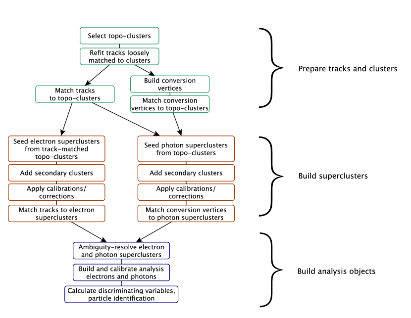
The reconstruction of electrons and photons with proceeds as shown in Figure 1. The algorithm first prepares the tracks and clusters it will use. It selects clusters of energy deposits measured in topologically connected EM and hadronic calorimeter cells [4], denoted topo-clusters, reconstructed as described in Section 4.1. These clusters are matched to ID tracks, which are re-fitted accounting for bremsstrahlung. The algorithm also builds conversion vertices and matches them to the selected topo-clusters. The electron and photon supercluster-building steps then run separately using the matched clusters as input. After applying initial position corrections and energy calibrations to the resulting superclusters, the supercluster-building algorithm matches tracks to the electron superclusters and conversion vertices to the photon superclusters. The electron and photon objects to be used for analyses are then built, their energies are calibrated, and discriminating variables used to separate electrons or photons from background are added.
The steps are described in more detail below.
4.1 Topo-cluster reconstruction
The topo-cluster reconstruction algorithm [26, 4] begins by forming proto-clusters in the EM and hadronic calorimeters using a set of noise thresholds in which the cell initiating the cluster is required to have significance , where
is the cell energy at the EM scale444The EM scale is the basic signal scale accounting correctly for the energy deposited in the calorimeter by electromagnetic showers. and is the expected cell noise. The expected cell noise includes the known electronic noise and an estimate of the pile-up noise corresponding to the average instantaneous luminosity expected for Run 2. In this initial stage, cells from the presampler and the first LAr EM calorimeter layer are excluded from initiating proto-clusters, to suppress the formation of noise clusters. The proto-clusters then collect neighbouring cells with significance . Each neighbour cell passing the threshold of becomes a seed cell in the next iteration, collecting each of its neighbours in the proto-cluster. If two proto-clusters contain the same cell with above the noise threshold, these proto-clusters are merged. A crown of nearest-neighbour cells is added to the cluster independently on their energy. In the presence of negative-energy cells induced by the calorimeter noise, the algorithm uses instead of to avoid biasing the cluster energy upwards, which would happen if only positive-energy cells were used. This set of thresholds is commonly known as ‘4-2-0’ topo-cluster reconstruction. Proto-clusters with two or more local maxima are split into separate clusters; a cell is considered a local maximum when it has , at least four neighbours, and when none of the neighbours has a larger signal.
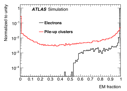
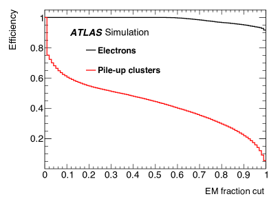
Electron and photon reconstruction starts from the topo-clusters but only uses the energy from cells in the EM calorimeter, except in the transition region of , where the energy measured in the presampler and the scintillator between the calorimeter cryostats is also added. This is referred to as the EM energy of the cluster, and the EM fraction () is the ratio of the EM energy to the total cluster energy. Only clusters with EM energy greater than are considered. The distribution of is shown in Figure 2(a) and the electron reconstruction efficiency for various cuts on is shown in Figure 2(b), for electron clusters which have been simulated with , and for pile-up clusters. A preselection requirement of was chosen for the initial topo-clusters, as it rejects of pile-up clusters without affecting the efficiency for selecting true electron topo-clusters.555In the transition region, some topo-clusters are also selected as EM clusters, even if they fail the requirement on , when they satisfy , in order to increase the reconstruction efficiency in that region. These clusters are referred to as EM topo-clusters in the rest of this paper.
4.2 Track reconstruction, track–cluster matching, and photon conversion reconstruction
Track reconstruction for electrons is unchanged with respect to Ref. [2, 1]. A summary of the changes applied for photons is given below.
Standard track-pattern reconstruction [27] is first performed everywhere in the inner detector. However, fixed-size clusters in the calorimeter that have a longitudinal and lateral shower profile compatible with that of an EM shower are used to create regions-of-interest (ROIs). If the standard pattern recognition fails for a silicon track seed (a set of silicon detector hits used to start a track) within an ROI, a modified pattern recognition algorithm based on a Kalman filter formalism [28] is used, allowing for up to 30% energy loss at each material intersection. Track candidates are then fitted with the global fitter [29], allowing for additional energy loss when the standard track fit fails. Additionally, tracks with silicon hits loosely matched666The match must be within and when using the track energy to extrapolate from the last inner detector hit, or and when using the cluster energy to extrapolate from the track perigee; refers to the reconstructed charge of the track. to fixed-size clusters are re-fitted using a Gaussian sum filter (GSF) algorithm [30], a non-linear generalization of the Kalman filter, for improved track parameter estimation.
The loosely matched, re-fitted tracks are then matched to the EM topo-clusters described above, extrapolating the track from the perigee to the second layer of the calorimeter, and using either the measured track momentum or rescaling the magnitude of the momentum to match the cluster energy. The momentum rescaling is performed to improve track–cluster matching for electron candidates with significant energy loss due to bremsstrahlung radiation in the tracker. A track is considered matched if, with either momentum magnitude, and , where refers to the reconstructed charge of the track. The requirement on is asymmetric because tracks sometimes miss some energy from radiated photons that clusters measure.
If multiple tracks are matched to a cluster, they are ranked as follows. Tracks with hits in the pixel detector are preferred, then tracks with hits in the SCT but not in the pixel detector. Within each category, tracks with a better match to the cluster in the second layer of the calorimeter are preferred, unless the differences are small (less than 0.01). The extrapolation of the track through the calorimeter is done first with the track momentum rescaled to the cluster energy and successively without rescaling. If both the first and the second extrapolation result in small differences, the track with more pixel hits is preferred, giving an extra weight to a hit in the innermost layer. The highest-ranked track is used to define the reconstructed electron properties.
The photon conversion reconstruction is largely unchanged from the method described in Ref. [1]. Tracks loosely matched to fixed-size clusters serve as input to the reconstruction of the conversion vertex. Both tracks with silicon hits (denoted Si tracks) and tracks reconstructed only in the TRT (denoted TRT tracks) are used for the conversion reconstruction. Two-track conversion vertices are reconstructed from two opposite-charge tracks forming a vertex consistent with that of a massless particle, while single-track vertices are essentially tracks without hits in the innermost sensitive layers. To increase the converted-photon purity, the tracks used to build conversion vertices must have a high probability to be electron tracks as determined by the TRT [31]. The requirement is loose for Si tracks but tight for TRT tracks used to build double-track conversions, and even tighter for tracks used to build single-track conversions.
Changes were made with respect to the reconstruction software described in Ref. [1], both to improve the reconstruction efficiency of double-track Si conversions (conversions reconstructed with two Si tracks), and to reduce the fraction of unconverted photons mistakenly reconstructed as single- or double-track TRT conversions (conversions reconstructed with one or two TRT tracks). The efficiency for double-track Si conversions was improved by modifying the tracking ambiguity processor, which determines which track seeds are retained to reconstruct tracks. For double-track conversion topologies, the two tracks are expected to be close to each other, parallel, and potentially to have shared hits, so that frequently only one track is reconstructed. The optimization in the ambiguity processor results in the recovery of the second track that was previously discarded. Overall, these modifications result in a – improvement in efficiency for double-track Si conversions, with larger improvements of up to for photons with conversion radii larger than 200 mm. In addition to reconstructing the second track of what would otherwise have been single-track Si conversions, the overall conversion reconstruction efficiency is improved by about by reducing the fraction of low-radius converted photons that are only reconstructed as electrons.
To reduce the fraction of unconverted photons reconstructed as double- or single-track TRT conversions, requirements on the TRT tracks were tightened. The tracks are required to have at least precision hits, where a precision hit is defined as a hit with a track-to-wire distance within 2.5 times its uncertainty [32]. In addition, the requirement on the probability of a track to correspond to an electron, as determined by the TRT, was tightened to 0.75 for tracks used in double-track TRT conversions and to 0.85 for tracks used in single-track TRT conversions, compared with the previous requirement of 0.7 for tracks used in both conversion types. The fraction of unconverted photons erroneously reconstructed as converted photons is below for events with , improving by a factor of two compared to the previous algorithm.
The conversion vertices are then matched to the EM topo-clusters.777If the conversion vertex has tracks with silicon hits, a conversion vertex is considered matched if, after extrapolation, the tracks match the cluster to within and . If the conversion vertex is made of only TRT tracks, then if the first track is in the TRT barrel, a match requires and , and if the first track is in the TRT endcap, a match requires and . If there are multiple conversion vertices matched to a cluster, double-track conversions with two silicon tracks are preferred over other double-track conversions, followed by single-track conversions. Within each category, the vertex with the smallest conversion radius is preferred.
4.3 Supercluster reconstruction
The reconstruction of electron and photon superclusters proceeds independently, each in two stages: in the first stage, EM topo-clusters are tested for use as seed cluster candidates, which form the basis of superclusters; in the second stage, EM topo-clusters near the seed candidates are identified as satellite cluster candidates, which may emerge from bremsstrahlung radiation or topo-cluster splitting. Satellite clusters are added to the seed candidates to form the final superclusters if they satisfy the necessary selection criteria.
The steps to build superclusters proceed as follows. The initial list of EM topo-clusters is sorted according to descending , calculated using the EM energy.888An exception to the ordering is made for clusters in the transition region that fail the standard selection but pass a looser selection; these are added at the end. The clusters are tested one by one in the sort order for use as seed clusters. For a cluster to become an electron supercluster seed, it is required to have a minimum of 1 GeV and must be matched to a track with at least four hits in the silicon tracking detectors. For photon reconstruction, a cluster must have greater than 1.5 GeV to qualify as a supercluster seed, with no requirement made on any track or conversion vertex matching. A cluster cannot be used as a seed cluster if it has already been added as a satellite cluster to another seed cluster.
If a cluster meets the seed cluster requirements, the algorithm attempts to find satellite clusters, using the process summarized in Figure 3.

For both electrons and photons, a cluster is considered a satellite if it falls within a window of around the seed cluster barycentre, as these cases tend to represent secondary EM showers originating from the same initial electron or photon. For electrons, a cluster is also considered a satellite if it is within a window of around the seed cluster barycentre, and its ‘best-matched’ track is also the best-matched track for the seed cluster. For photons with conversion vertices made up only of tracks containing silicon hits, a cluster is added as a satellite if its best-matched (electron) track belongs to the conversion vertex matched to the seed cluster. These steps rely on tracking information to discriminate distant radiative photons or conversion electrons from pile-up noise or other unrelated clusters.
The seed clusters with their associated satellite clusters are called superclusters. The final step in the supercluster-building algorithm is to assign calorimeter cells to a given supercluster. Only cells from the presampler and the first three LAr calorimeter layers are considered, except in the transition region of , where the energy measured in the scintillator between the calorimeter cryostats is also added. To limit the superclusters’ sensitivity to pile-up noise, the size of each constituent topo-cluster is restricted to a maximal width of 0.075 or 0.125 in the direction in the barrel or endcap region, respectively. Because the magnetic field in the ID is parallel to the beam-line, interactions between the electron or photon and detector material generally cause the EM shower to spread in the direction, so the restriction in still generally allows the electron or photon energy to be captured. No restriction is applied in the -direction.
4.4 Creation of electrons and photons for analysis
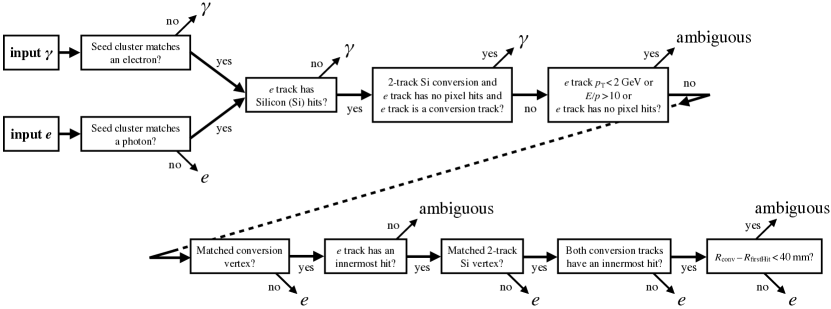
After the electron and photon superclusters are built, an initial energy calibration and position correction is applied to them, and tracks are matched to electron superclusters and conversion vertices to photon superclusters. The matching is performed the same way that the matching to EM topo-clusters was performed, but using the superclusters instead. Creating the analysis-level electrons and photons follows. Because electron and photon superclusters are built independently, a given seed cluster can produce both an electron and a photon. In such cases, the procedure presented in Figure 4 is applied. The purpose is that if a particular object can be easily identified only as a photon (a cluster with no good track attached) or only as an electron (a cluster with a good track attached and no good photon conversion vertex), then only a photon or an electron object is created for analysis; otherwise, both an electron and a photon object are created. Furthermore, these cases are marked explicitly as ambiguous, allowing the final classification of these objects to be determined based upon the specific requirements of each analysis.
Because the energy calibration depends on matched tracks and conversion vertices, and the initial supercluster calibration is performed before the final track and conversion matching, the energies of the electrons and photons are recalibrated, following the procedure described in Ref. [3].
Subsequently, shower shape and other discriminating variables [2, 1] are calculated for electron and photon identification. A list is given in Table 1, along with an indication if they are used for electron or photon identification. The lateral shower shapes are based on the position of the most energetic cell, so they are independent of the clustering used, provided the same most energetic cell is included in the clusters. More information about the variables and the identification methods are given in Sections 6 and 7 for electrons and photons, respectively.
| Category | Description | Name | Usage |
|---|---|---|---|
| Hadronic leakage | Ratio of in the first layer of the hadronic calorimeter to of the EM cluster (used over the ranges and ) | ||
| Ratio of in the hadronic calorimeter to of the EM cluster (used over the range ) | |||
| EM third layer | Ratio of the energy in the third layer to the total energy in the EM calorimeter | ||
| EM second layer | Ratio of the sum of the energies of the cells contained in a rectangle (measured in cell units) to the sum of the cell energies in a rectangle, both centred around the most energetic cell | ||
| Lateral shower width, , where is the energy and is the pseudorapidity of cell and the sum is calculated within a window of cells | |||
| Ratio of the sum of the energies of the cells contained in a rectangle (measured in cell units) to the sum of the cell energies in a rectangle, both centred around the most energetic cell | |||
| EM first layer | Total lateral shower width, , where runs over all cells in a window of and is the index of the highest-energy cell | ||
| Lateral shower width, , where runs over all cells in a window of 3 cells around the highest-energy cell | |||
| Energy fraction outside core of three central cells, within seven cells | |||
| Difference between the energy of the cell associated with the second maximum, and the energy reconstructed in the cell with the smallest value found between the first and second maxima | |||
| Ratio of the energy difference between the maximum energy deposit and the energy deposit in a secondary maximum in the cluster to the sum of these energies | |||
| Ratio of the energy measured in the first layer of the electromagnetic calorimeter to the total energy of the EM cluster | |||
| Track conditions | Number of hits in the innermost pixel layer | ||
| Number of hits in the pixel detector | |||
| Total number of hits in the pixel and SCT detectors | |||
| Transverse impact parameter relative to the beam-line | |||
| Significance of transverse impact parameter defined as the ratio of to its uncertainty | || | ||
| Momentum lost by the track between the perigee and the last measurement point divided by the momentum at perigee | |||
| Likelihood probability based on transition radiation in the TRT | eProbabilityHT | ||
| Track–cluster matching | between the cluster position in the first layer of the EM calorimeter and the extrapolated track | ||
| between the cluster position in the second layer of the EM calorimeter and the momentum-rescaled track, extrapolated from the perigee, times the charge | |||
| Ratio of the cluster energy to the measured track momentum |
4.5 Performance
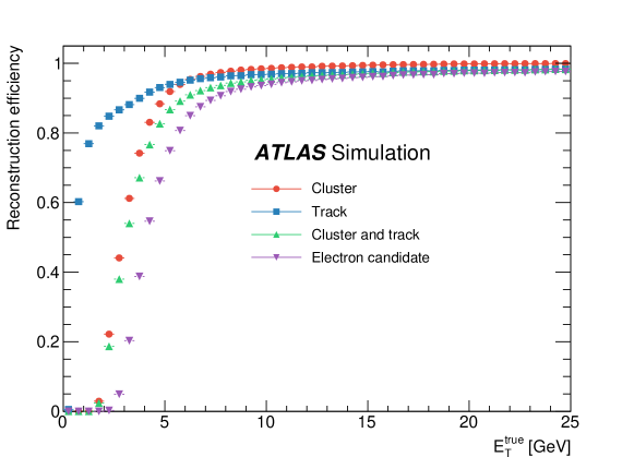
Figure 5 shows the reconstruction efficiencies for electrons. The reconstruction efficiency at high approaches the tracking efficiency, as expected. One interesting feature, however, is the difference between the efficiency to reconstruct the cluster and track (green triangles) and the efficiency to reconstruct an electron (purple inverted triangles) at lower . The reason for this is that tracks with silicon hits are considered for matching to superclusters only if they have had a GSF re-fit performed. The fixed-size clusters used for choosing the tracks on which the GSF re-fit is performed introduce an threshold, which is the source of this inefficiency. To alleviate this feature, the EM topo-clusters as defined in Section 4.1 could be used to seed the GSF fit.
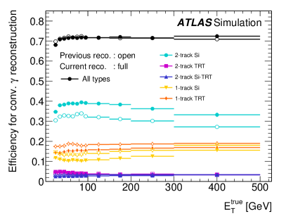
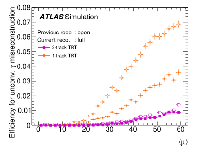
The top plot in Figure 6 shows the reconstruction efficiency for converted photons as a function of the true of the simulated photon for the previous version of the reconstruction software, described in Ref. [1], and the current version, described in Section 4.2, along with the contributions of the different conversion types. For a photon to be classified as a true converted photon, the true radius of the conversion must be smaller than . Only simulated photons with transverse energy greater than 20 GeV are considered. The simulated photons are distributed uniformly in , with most of the photons having a transverse momentum smaller than 200 GeV. The bottom left plot of Figure 6 shows the reconstruction efficiency for converted photons along with the contributions of the different conversion types as a function of . The improvement (see Section 4.2) in the reconstruction efficiency for double-track Si conversions and the corresponding reduction of single-track Si conversions is clearly visible in those two plots. A slight reduction in double- and single-track TRT conversion efficiency is also visible, with the purpose of significantly reducing the probability for true unconverted photons to be reconstructed as TRT conversions, as can be seen in the bottom right plot of Figure 6. The probability for true unconverted photons to be reconstructed as Si conversions is negligible in comparison.

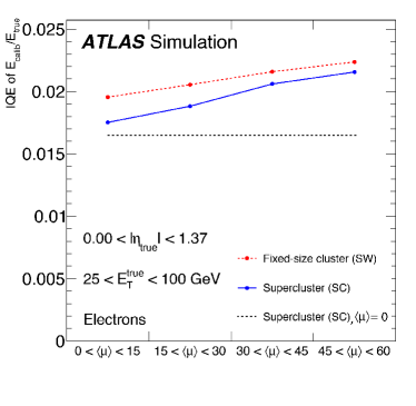
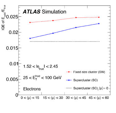
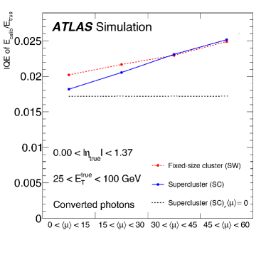
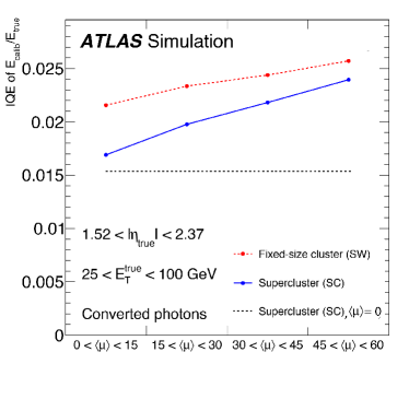
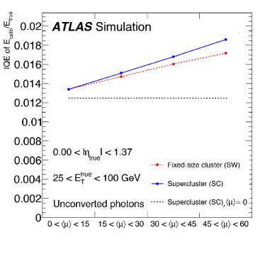
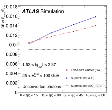
An important reason for using superclusters is the improved energy resolution that superclusters provide by collecting more of the deposited energy. The peaks of the energy response, , where is the true energy of the simulated particle prior to any detector simulation, and is the calibrated reconstructed energy, do not deviate from one by more than for the different particles. To quantify the width (resolution) of the energy response, the effective interquartile range is used, defined as
where and are the first and third quartiles of the distribution of , and the normalization factor is chosen such that the IQE of a Gaussian distribution would equal its standard deviation.
Comparisons of the resolutions of the calibrated energy response of simulated single electrons, converted photons, and unconverted photons, built using fixed-size clusters and superclusters, are given in Figure 7. In particular, Figure 7 shows the IQE of the two approaches in different regions of and . The reconstructed electrons and photons in these distributions are required to correspond to true primary electrons and photons and to satisfy loose identification requirements. After calibration, the supercluster algorithm shows a significant improvement in resolution compared with the sliding-window algorithm for electrons. In absence of pile-up, an improvement in resolution of up to – is found in some bins in the endcap region of the detector, as well as in the central region for low- electrons.
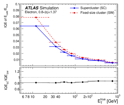
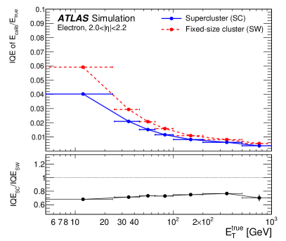
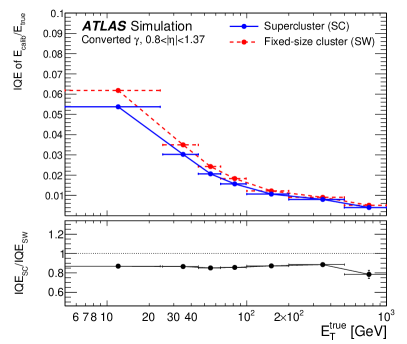

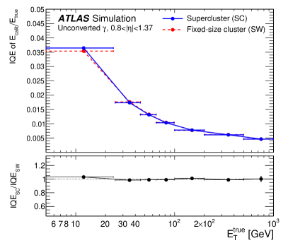
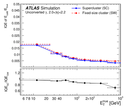
Similarly, a large improvement in the resolution is seen for converted photons, over in a few bins. For unconverted photons, the overall change in performance is small, due to the generally narrower shower width. However, some improvement is observed for high bins in the endcap region. In presence of pile-up, the improvement in resolution still reaches 15 to 20%, depending on and .
An important consideration is the performance of the supercluster reconstruction at different pile-up levels. Figure 8 shows the calibrated energy response resolution at different levels for electrons, converted photons, and unconverted photons, in two regions.
The topo-cluster noise thresholds for the ‘high-’ data sample were tuned for . For electrons and converted photons, the IQE of the supercluster reconstruction generally remains better, although the supercluster-based response is more sensitive to pile-up, as seen by its larger slope as a function of . Part of the reason is that the topo-cluster noise thresholds remain fixed even though changes. For unconverted photons, however, the supercluster reconstruction shows worse IQE for . This degradation could be mitigated in particular by limiting the growth of the size of the clusters.
5 Electron and photon energy calibration
The energy calibration of electrons and photons closely follows the procedure used in Ref. [3], updated for the new energy reconstruction described in Section 4. The energy resolution of the electron or photon is optimized using a multivariate regression algorithm based on the properties of the shower development in the EM calorimeter. The adjustment of the absolute energy scale using decays is updated, together with systematic uncertainties related to pile-up and material effects. The universality of the energy scale is verified using radiative -boson decays.
5.1 Energy scale and resolution measurements with decays
The difference in energy scale between data and simulation is defined as , where corresponds to different regions in . Similarly, the mismodelling of the energy resolution is parameterised as an -dependent additional constant term, . The corresponding energy scale correction is applied to the data, and the resolution correction is applied to the simulation as follows:
where the symbol denotes a sum in quadrature.
For samples of decays, with electrons reconstructed in regions and , the effect of the energy scale correction on the dielectron invariant mass is given in first order by , with . Similarly, the difference in the simulated mass resolution is given by , with . The values of and are determined by optimizing the agreement between the invariant mass distributions in data and simulation, separately for each category. The and parameters are then extracted from a simultaneous fit of all categories.
Two methods are used for this comparison and the difference is taken as a systematic uncertainty. In the first method, the best estimates of and are found by minimizing the of the difference between data and simulation templates. The templates are created by shifting the mass scale in simulation by and by applying an extra resolution contribution of . In the second method, used as a cross-check, a sum of three Gaussian functions is fitted to the data and simulated invariant mass distributions in each region; the and are extracted from the differences, between data and simulation, of the means and widths of the fitted distributions.
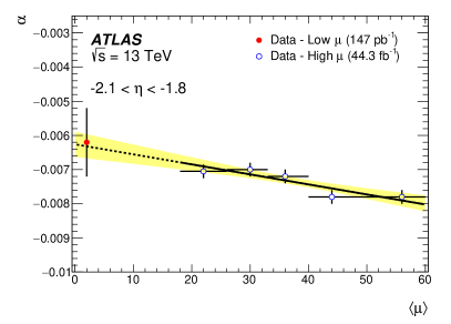
Figures 9 (a) and (b) show the results of and derived in 68 and 24 intervals, respectively, separately for 2015, 2016 and 2017. The difference in for the different years is mainly due to two effects: variations of the LAr temperature, and the increase of the instantaneous luminosity. The former effect induces a variation in the charge/energy collection, affecting the energy response by about –2%/K [33]. The latter implies an increased amount of deposited energy in the liquid-argon gap that creates a current in the high-voltage lines, reducing the high voltage effectively applied to the gap and introducing a variation of the response of up to 0.1 in the endcap region. A prediction of the different effects that can impact the results is presented in Ref. [3]. Given the small size of the observed dependence, well within 0.3%, dedicated energy scale corrections for each data taking year provide an adequate stability of the energy measurement.
For the constant term corrections , a dependence on the pile-up level is observed through the different values obtained for 2015 to 2017 data; this is addressed in Section 5.2. A weighted average of the values for the different years is applied in the analyses of the complete dataset. The additional constant term of the energy resolution is typically less than 1 in most of the barrel and between 1 and 2 in the endcap.
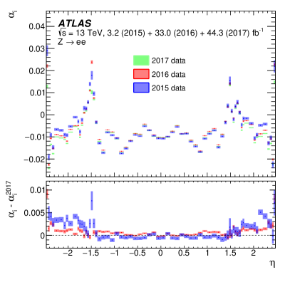
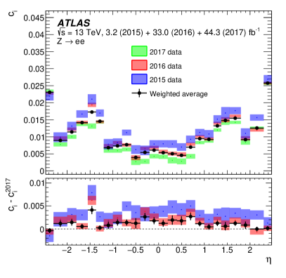
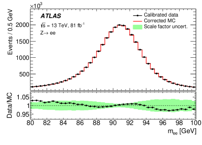
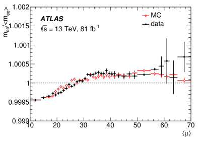
Figure 10(a) shows the invariant mass distribution for candidates for data and simulation after the energy scale correction has been applied to the data and the resolution correction to the simulation. No background contamination is taken into account in this comparison, but it is expected to be at the level of 1 over the full shown mass range. The uncertainty band corresponds to the propagation of the uncertainties in the and factors, as discussed in Ref. [3]. Within these uncertainties, the data and simulation are in fair agreement. Figure 10(b) shows the stability of the reconstructed peak position of the dielectron mass distribution as a function of the average number of interactions per bunch crossing for the data collected in 2015, 2016 and 2017. The variation of the energy scale with is well below the 0.1 level in the data. The small increase of energy with observed in data is consistent with the MC expectation and is related to the new dynamical clustering used for the energy measurement, as introduced in Section 4.
5.2 Systematic uncertainties
Several systematic uncertainties impact the measurement of the energy of electrons or photons in a way that depends on their transverse energy and pseudorapidity. These uncertainties were evaluated in Ref. [3]. The amount of passive material located between the interaction point and the EM calorimeter is measured using the ratio of the energies deposited by electrons from -boson decays in the first and second layer of the EM calorimeter (). The sensitivity of the calibrated energy to the detector material was re-evaluated to reflect the changes in the reconstruction described above. The systematic uncertainty due to the material description of the innermost pixel detector layer and the services of the pixel detector were updated with regards to Ref. [3] using a more accurate description of these systems in the simulation [34].
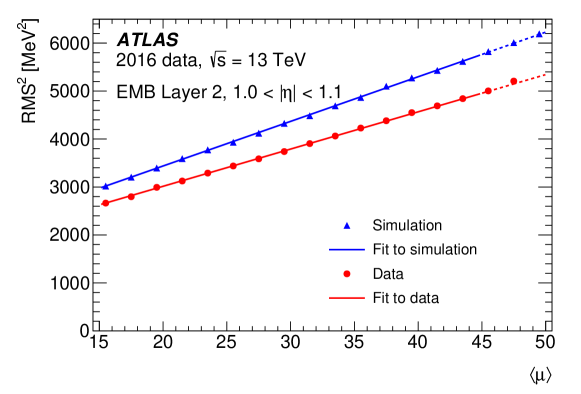
The dependence of the constant term on the amount of pile-up, observed in Figure 9(b), is explained by the larger pile-up noise predicted by the simulation, compared with that observed in the data. Figure 11 shows an example of the evolution of the second central moment of the cell energy deposit in data and simulation as a function of for the second layer and assuming symmetry. The contribution of the pile-up noise varies linearly with , while the electronic noise remains constant. An average difference of 10 between the pile-up noise in data and simulation is observed. This mismodelling is absorbed in the parameters for electrons of GeV, the average value for electrons from decays used to derive the energy corrections. The two methods used for the extraction of the energy resolution corrections, described in Section 5.1, are compared and the full difference is taken as an uncertainty in the energy resolution. This uncertainty amounts to up to in the barrel and is due to the different sensitivities of the two methods to the pile-up. The impact of a 10 difference in pile-up noise at a different energy is propagated to the energy resolution uncertainty relying on the predicted dependence of the pile-up noise effect as a function of the energy. For electrons and photons in the transverse energy range 30–60 GeV, the uncertainty in the energy resolution is of the order of to . In order to mimic the pile-up noise estimation in the simulation, the pile-up rescaling factor, described in Section 3, is changed from 1.03 to 1.2 for the 48b filling scheme and to 1.3 for the 8b4e filling scheme. A systematic uncertainty in the energy scale is derived comparing the results obtained with the two pile-up reweighting factors; it is of the order of in the barrel and of in the endcap. The total systematic uncertainty in the energy scale amounts to in the barrel and in the endcap.
5.3 Validation of the photon energy scale with decays
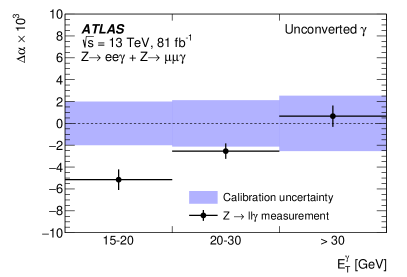
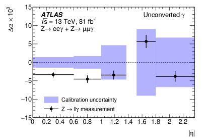
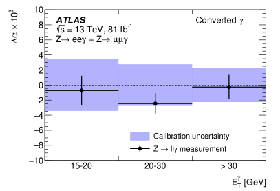
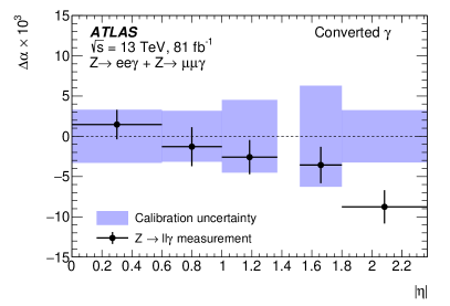
The energy scale corrections extracted from decays, as described in Section 5.1, are applied to correct the photon energy scale. A data-driven validation of the photon energy scale corrections is performed using radiative decays of the boson, probing mainly the low-energy region. Residual energy scale factors for photons, , are derived by comparing the mass distribution of the system in data and simulation after applying the -based energy scale corrections. The mass distribution of the system in the simulation is modified by applying to the photon energy and the value of that minimizes the comparison between the data and the simulation is extracted. If the energy calibration is correct, should be consistent with zero within the uncertainties described in Section 5.2. An alternative method based on a binned extended maximum-likelihood fit with an analytic function to describe the mass distribution is used, and gives consistent results. The electron and muon channels are analysed separately. In the electron channel, the electron energy scale uncertainty is accounted for in the determination of the residual photon energy scale. The electron and muon results are found to agree, and are combined. Figure 12 shows the measured as a function of and , separately for converted and unconverted photons. The dominant sources of uncertainty in the extrapolation to photons of the energy corrections derived in decays are related to the amount of passive material in front of the EM calorimeter, and to the intercalibration of the calorimeter layers. The value of is consistent with zero within about two standard deviations at most.
5.4 Energy scale and resolution corrections in low-pile-up data
Special data with low pile-up were collected in 2017 at 13 TeV, as described in Section 3. Energy scale factors are derived for this sample using the baseline method, described in Section 5.1. The measurement is done in 24 regions given the small size of the sample.
An alternative approach, used for validation, consists of measuring the energy scale factors using high-pile-up data and extrapolating the results to the low-pile-up conditions. Two main effects are considered in the extrapolation, namely the explicit dependence of the energy corrections on , and differences between the clustering thresholds used for the two samples; other effects are sub-leading and are treated as systematic uncertainties.
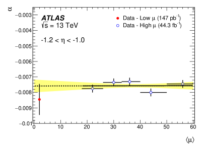
To evaluate the first effect, the high-pile-up energy scale corrections are measured in five intervals of in the range , in each of the 24 regions considered for the low-pile-up sample. The results are parameterized using a linear function, which is extrapolated to . Over this range, the energy correction is found to vary by about 0.01% in the barrel, and by about 0.1% in the endcap. The statistical uncertainty in the extrapolation is about 0.05% in each region. The procedure is illustrated in Figure 13, for representative regions in the barrel and in the endcap.
Secondly, as described in Section 4, the low-pile-up data were reconstructed with topo-cluster noise thresholds corresponding to , while the standard runs used thresholds corresponding to . This results in an increased cluster size and enhanced energy response for the low-pile-up samples. The difference between the enhancements in data and simulation is measured using -boson decays, and a correction applied. The correction amounts to about in the barrel and in the endcap, with a typical uncertainty of .
Figure 14(a) shows the comparison between the energy scale factors derived from low-pile-up data and extrapolated from high-pile-up data after correcting for the noise threshold effect. The observed difference is of the order of in the barrel region and increases to in the endcap region.
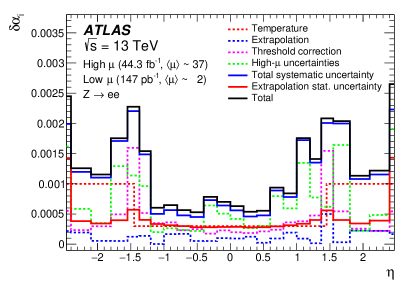
Different systematic uncertainties were considered for the extrapolation approach. In addition to the systematic uncertainties in high-pile-up data discussed in Section 5.2, systematic uncertainties related to the functional form chosen for the extrapolation or the number of intervals considered were evaluated and are of the order of a few . The changes of the LAr temperature, in the absence of collisions, between the low-pile-up and high-pile-up data-taking periods, was found to induce a variation of the energy scale by 0.006%. A systematic uncertainty in the energy scale is also added for the non-linear variation of the LAr temperature with and amounts to a few times in the barrel and in the endcap. The total uncertainty in the extrapolated energy scale factors is about 0.05% in the barrel, and on average 0.15% in the endcap, as shown in Figure 14(b).

6 Electron identification
Further quality criteria, called ‘identification selections’ below, are used to improve the purity of selected electron and photon objects. The identification of prompt electrons relies on a likelihood discriminant constructed from quantities measured in the inner detector, the calorimeter and the combined inner detector and calorimeter. A detailed description is given in Ref. [2]. Recent changes implemented as a result of the migration to the supercluster reconstruction algorithm and adjustments made in parallel are discussed in the following. The identification criteria apply to all reconstructed electron candidates (see Section 4).
6.1 Variables in the electron identification
The quantities used in the electron identification are chosen according to their ability to discriminate prompt isolated electrons from energy deposits from hadronic jets, from converted photons and from genuine electrons produced in the decays of heavy-flavour hadrons. The variables can be grouped into properties of the primary electron track, the lateral and longitudinal development of the electromagnetic shower in the EM calorimeter, and the spatial compatibility of the primary electron track with the reconstructed cluster. They are described in Table 1 and summarized here.
The primary electron track is required to fulfil a set of quality requirements, namely hits in the two inner tracking layers closest to the beam line, as well as a number of hits in the silicon-strip detectors. The transverse impact parameter of the track and its significance are used to construct the likelihood discriminant. Furthermore, and particle identification in the TRT are used.
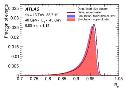
The lateral development of the electromagnetic shower is characterized with variables calculated separately in the first and second layer of the electromagnetic calorimeter. To reject clusters from multiple incident particles, is used (see Table 1). The lateral shower development is measured with and . All lateral shower shape variables are calculated by summing energy deposits in calorimeter cells relative to the cluster’s most energetic cell, and no significant difference between fixed-size EM clusters and superclusters is expected in these variables, as shown in Figure 15(a) for .
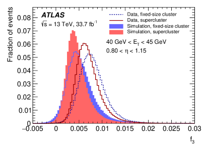
For the longitudinal shower shape variables, the numbers of cells contributing to the energy measurement in each layer are chosen dynamically in the supercluster approach, compared with fixed numbers of cells in fixed-size clusters. The supercluster approach inherently suppresses noise in the calorimeter cells, resulting in lower values and narrower distributions. The electron identification uses and (see Table 1). The distribution of is compared for fixed-size clusters and superclusters in Figure 15(b). The significant differences between data and simulation are caused by a known mismodelling of calorimeter shower shapes in the Geant4 detector simulation. These are accounted for in the optimisation of the electron identification (see Section 6.3) and corrected with data-to-simulation efficiency ratios in analyses. Further discrimination against hadronic showers is achieved with .
The reconstructed track and the EM cluster are matched using and .
6.2 Likelihood discriminant
A discriminant is formed from the likelihoods for a reconstructed electron to originate from signal, , or background, . They are calculated from probability density functions (pdfs), , which are created by smoothing histograms of the (typically 13) discriminating variables with an adaptive kernel density estimator (KDE [35]) as implemented in TMVA [36], separately for signal and background and in 9 bins in and 7 bins of :
For signal and background the pdfs take the values and , respectively, for the quantity at value . The likelihood discriminant is defined as the natural logarithm of the ratio of and .
The pdfs for signal were derived from (for GeV) and events (for GeV) prior to the 2017 data-taking period in fb-1 of data recorded in the years 2015 and 2016. A reconstructed electron is selected in these events using a tag-and-probe method [37]. One of the electrons must satisfy a strict requirement on the likelihood discriminant of the previous electron identification [2] and the other electron serves as a probe. To reduce the background contamination in the selected data, probe electrons are required to satisfy a very loose requirement on the likelihood discriminant. This requirement rejects approximately 95% of the background with a signal efficiency of 97%, causing only a mild distortion of the likelihood pdfs. Events with at least one reconstructed electron are selected to derive the pdfs for background. This sample primarily contains dijet events; contributions from genuine electrons, mainly from and decays, are suppressed to a negligible level using dedicated selection criteria. Deriving the likelihood pdfs in data is an improvement compared to the previous likelihood-based identification, which used simulation. Compared to the mismodelling in simulation, the selection applied in data and differences in the run conditions between the years 2015, 2016, 2017 and 2018 cause only mild differences in the pdfs.
The electron likelihood identification imposes a selection on the likelihood discriminant and some additional requirements. The variable exhibits a dependence on the electron and that cannot adequately be captured by the seven and nine bins, respectively, in which the pdfs are determined. It is therefore only used for electrons with and GeV. Electrons are also rejected if a two-track silicon conversion vertex was reconstructed with a momentum closer to the cluster energy than that of the primary electron track. To pass the Tight operating point, electrons must moreover satisfy and their primary track must satisfy GeV. These additional criteria aim to reject background from converted photons. For very high the energy dependence of the shower shape variables can cause a degradation of efficiencies for very strict requirements on the likelihood discriminant. To avoid efficiency losses in the Tight identification, the cuts on are chosen to be identical to the Medium identification for GeV, and the operating points differ only in the additional requirements and an -dependent requirement on the shower width in the first calorimeter layer, applied to Tight electrons.
6.3 Efficiency of the electron identification
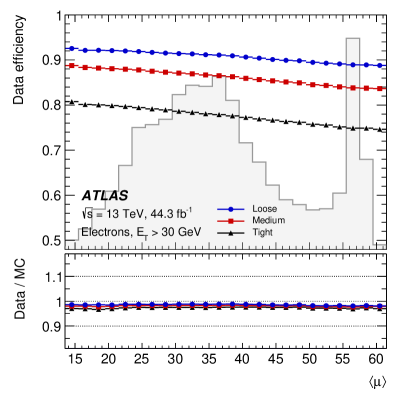
The operating points Loose, Medium and Tight are each optimized in 9 bins in and 12 bins in such that reconstructed electrons meet the requirements on the likelihood discriminant with some predefined efficiency. The values of these requirements are determined in simulated events. For that purpose, the electromagnetic shower quantities and the combined track–cluster variables are shifted and adjusted in width such that the resulting distribution of the likelihood discriminant of the simulated electrons closely matches that in data. The discriminant threshold is adjusted linearly as a function of pile-up level to yield a stable rejection of background electrons. The number of reconstructed vertices serves as a measure for pile-up. Due to the deterioration of the discriminating power with pile-up, the approximately constant background rejection is accompanied by a reduction of signal efficiency as a function of the average number of interactions per bunch crossing, as shown in Figure 16 for a pure sample of electrons from -boson decays.
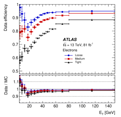
The target efficiencies are the same as in the previous identification [2], as these have proven to suit a wide range of analyses and topologies. For typical electroweak processes they are, on average, 93%, 88% and 80% for the Loose, Medium, and Tight operating points and gradually increase from low to high . The reduced efficiency of the Medium and Tight operating points is accompanied by an improved rejection of background processes by factors of approximately 2.0 and 3.5, respectively, in the range GeV. The background efficiency was evaluated in QCD two-to-two processes simulated as described in Section 3.1. Figure 17 shows the resulting efficiencies in data. With increasing , the identification efficiency varies from 58% at GeV to 88% at GeV for the Tight operating point, and from 86% at GeV to 95% at GeV for the Loose operating point. In 2015, a different gas mixture was used in the TRT causing higher efficiencies. Similar efficiencies are obtained for the data recorded in the years 2016 and 2017 and residual differences are caused by their dependence on pileup. The discontinuity in the efficiency curve at GeV is caused by a known mismodelling of the variables used in the likelihood discriminant at low : performing the optimization of the discriminant cuts using simulated events leads to a higher efficiency in data in this region, resulting in the rise at low observed in the lower panels of Figure 17.
The uncertainties in the efficiency are at and decrease with transverse energy, reaching better than for . The systematic uncertainties in the measurements are dominated by background subtraction uncertainties at low , and are derived as decribed in Ref. [2]. For larger values of , additional systematic uncertainties of , , assigned due to variations in the electron efficiency with for Loose, Medium and Tight identification, respectively, limit the precision.

7 Photon identification
7.1 Optimization of the photon identification
The photon identification criteria are designed to efficiently select prompt, isolated photons and reject backgrounds from hadronic jets. The photon identification is constructed from one-dimensional selection criteria, or a cut-based selection, using the shower shape variables described in Table 1. The variables using the EM first layer play a particularly important role in rejecting decays into two highly collimated photons.
The primary identification selection is labelled as Tight, with less restrictive selections called Medium and Loose, which are used for trigger algorithms. The Loose identification criteria have remained unchanged since the beginning of Run 2, and Loose was the main selection used in the triggering of photon and diphoton events in 2015 and 2016. It uses the , , , and shower shape variables. The Medium selection, which adds a loose cut on , became the main trigger selection in the beginning of 2017, in order to maintain an acceptable trigger rate. Because the reconstruction of photons in the ATLAS trigger system does not differentiate between converted and unconverted photons, the Loose and Medium identification criteria are the same for converted and unconverted photons. The Tight identification criteria described in this paper are designed to select a subset of the photon candidates passing the Medium criteria. Because the shower shapes vary due to the geometry of the calorimeter, the cut-based selection of Loose, Medium and Tight are optimized separately in bins of . The Tight identification presented here is also optimized in separate bins of , and compared with an earlier version of the Tight identification that makes an -independent selection.
The Tight identification is optimized using TMVA, and performed separately for converted and unconverted photons. The shower shapes of converted photons differ from unconverted photons due to the opening angle of the conversion pair, which is amplified by the magnetic field, and from the additional interaction of the conversion pair with the material upstream of the calorimeters.
The Tight identification is optimized using a series of MC samples that provide prompt photons and representative backgrounds at different transverse momenta. For photons with GeV, the MC sample with the selection described in Section 3.1 is used as a signal. The corresponding background sample is obtained from data consisting of +jets events collected using a similar event selection, but with relaxed requirements on the dilepton and dilepton+photon invariant masses and . Above GeV, the inclusive-photon production MC sample described in Section 3.2 is compared with a dijet background MC sample that is enriched in high- energy deposits using a generator-level filter. No isolation selection is applied to the training samples, and the shower shape variables are corrected to match the shower shapes observed in data using the correction procedure described in Ref. [1].
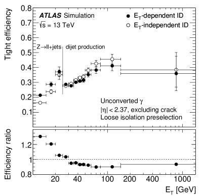
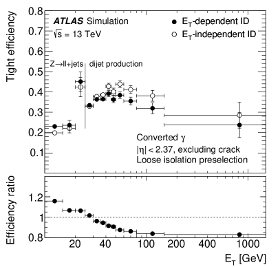
Figures 18 and 19 show the result of the Tight identification optimization in terms of the efficiencies as a function of for the signal and background MC training samples. The optimized selection, labelled -dependent, is compared with a reference selection that uses criteria that do not change with (-independent). The new, -dependent Tight identification allows the efficiencies of low- and high- photon regions to be tuned separately. The Tight identification is tuned to give a 20% higher efficiency at low , and an improved background rejection at high . The dependence of the photon identification is depicted in Figure 20 for photons from decays.
7.2 Efficiency of the photon identification
To assess the performance of the (-dependent) Tight photon identification on data, three photon efficiency measurements are performed using distinct data samples. The first uses an inclusive-photon production data selection, the second uses photons radiated from leptons in decays, and the third uses electrons from decays, with a method that transforms the electron shower shapes to resemble the photon shower shapes. These efficiency measurements are described in detail in Ref. [1], and summarized below. All three procedures measure photons that are isolated, using the Loose working-point definition (see Section 8.2).
The three measurements use a common method to characterize the imperfect modelling of shower shapes in simulated samples, in order to estimate its impact on the efficiency measurement in data. Nominally, the MC shower shapes are compared with data in control regions enriched in real photons and corrected by applying a simple shift to the distributions, whose magnitude is determined by a minimization procedure. However, some data–MC differences cannot be corrected by this procedure, such as the widths of the distributions. In order to estimate any residual data–MC differences, the minimisation is repeated considering only the tail of the distribution, defined as the region containing 30% of the distribution on the side closer to the identification cut value. The shift value obtained when comparing the data and simulation tails is used to define a systematic uncertainty in the modelling of the shower shapes, and is derived for all variables for which a mismodelling is observed. Four variations are defined using sets of correlated variables; the variables within each set are shifted together: {}, {}, {,}, and {,,}. The result is equivalent to four sets of MC simulated samples, which can be used to assign systematic uncertainties for mismodelling effects that impact the data measurement, and which are considered to be uncorrelated variations.
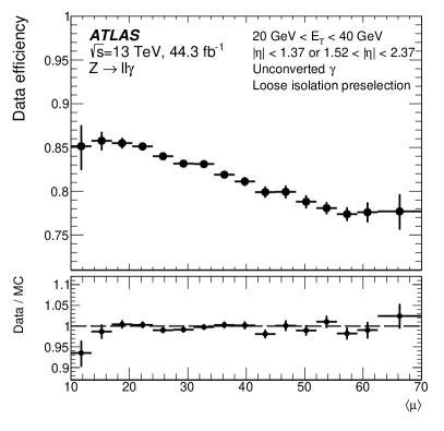
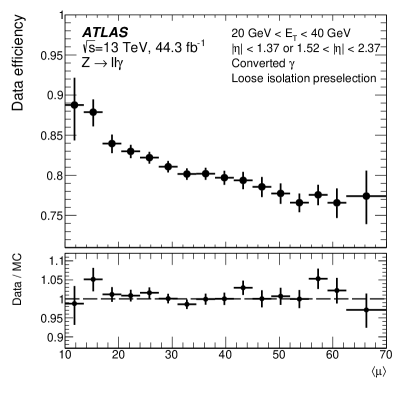
The method using decays selects data as described in Section 3.1. Additional requirements on the invariant mass of the three-body system, GeV, and on the lepton-pair invariant mass, GeV, select radiative -boson decays while rejecting backgrounds from and jets production. The efficiency and purity of the samples with and without the Tight identification requirement are determined from fits of signal and background templates, extracted from simulated and jets events, to the observed three-body invariant-mass distribution.
The systematic uncertainties in the photon efficiency measurement using decays include a closure test using simulated signal and background samples to assess the validity of the measurement. To assess the impact of simulation mismodelling, the measurement is repeated comparing the Powheg-Pythia8 and Sherpa samples and the difference is taken as a systematic uncertainty. The shower shape correction uncertainties are considered by repeating the measurement with each of the four sets of modified simulation samples, and the observed differences are added in quadrature. Finally, as a test of the background description, the fit range of the distribution is varied from its nominal value of [65,105] GeV using two variations, [45,95] GeV and [80,120] GeV, and the efficiency differences are assigned as a systematic uncertainty.
The method to extract the photon efficiency using inclusive-photon production relies on data collected with prescaled photon triggers that feature a Loose identification requirement, as described in Section 3.1. This data sample contains a mixture of real photons and backgrounds from jet production, and a matrix method is used to extract the photon efficiency. The matrix method constructs four regions by categorizing Loose photon candidates according to whether they pass or fail the Tight identification, and whether they pass or fail track-based isolation cuts. The four regions contain eight unknowns (i.e. the numbers of signal and background events in each region); if the isolation efficiencies for signal and background from each region are known, the efficiency for Loose photons to pass the Tight identification can be extracted. The isolation efficiencies for loosely and tightly identified signal photons are determined from the Monte Carlo samples, and the isolation efficiencies for backgrounds are obtained in a jet-enriched control region constructed by inverting identification criteria. Finally, the efficiency for reconstructed photon candidates to pass the Loose identification is determined from simulation, as this contribution is not measured in data by this method. The magnitude of the correction is typically less than 5%, and smaller at high .
Systematic uncertainties assigned to the matrix method include a closure uncertainty that quantifies the agreement between the background isolation efficiencies derived in the data control region and in the regions to which they are applied. This effect is estimated using simulation, and is the largest source of uncertainty in the measurement. The robustness of the method is tested by varying the track-based isolation requirement, and assigning any difference in measured efficiency as a systematic uncertainty. The impact of uncertainties in the shower shape corrections is estimated using simulation; the effects of the four shower shape variations described above are added in quadrature. Finally, an uncertainty is assigned for a potential mismodelling in the MC-based correction to extrapolate from Loose to reconstructed photons. This uncertainty is based on the Loose identification efficiency measured with radiative photons in events.
Photon efficiencies can be estimated in a data sample of electrons from decays whose shower shape variables have been modified to resemble photon shower shapes, a technique referred to as the electron extrapolation method. This efficiency measurement, described in Ref. [1], uses the sample defined in Section 3.1, with the photon Loose isolation requirement applied to the electron candidates. Electron shower shape variables are modified using a Smirnov transform [38] derived from simulated and inclusive-photon production samples. The candidate electrons in data contain a small background from jets and multijet production; this background is subtracted by fitting simulated signal samples and background templates derived from data control regions to the data distributions. The electron candidates are counted for events in the range GeV, and the efficiencies are measured using the tag-and-probe method as described in Section 6.
The systematic uncertainties in the electron extrapolation method are as follows. First, a closure test is performed to determine whether the transformed electrons can reproduce the expected photon efficiency, using the simulation and in the absence of background. The difference in relative efficiency, which can be as high as 3%, is applied as a correction to the measured data efficiency, and the magnitude of the correction is assigned as the systematic uncertainty. Systematic effects that affect the Smirnov transformations include the fraction of fragmentation photons in the simulated inclusive-photon sample, which is varied by %, and the predicted fraction of true converted photons, which is varied by %, to assess the impact of the imperfect simulation on the efficiency measurement. The uncertainty in the modelling of identification variables in simulation is assessed by defining Smirnov transformations for each of the four sets of variations of the shower shape modelling, recalculating the efficiency for each case; the total modelling uncertainty is taken as the sum in quadrature of the individual variations. The uncertainty due to the limited size of the MC samples used to derive the Smirnov transformations is assessed using the bootstrap method. Finally, the uncertainty associated with the subtraction of the jets and multijet backgrounds in the signal region is tested by reducing the level of background through a restriction of the selected invariant-mass range to GeV, and repeating the measurement procedure. The resulting difference in the measured efficiency is taken as the systematic uncertainty.
The three efficiency measurements are compared with MC simulation in order to obtain scale factors, in bins of and , that are used to correct the MC simulations so that the simulations closely resemble data. Before determining these scale factors, the shower shapes in these MC simulations were corrected to match data using the procedure described in Ref. [1].
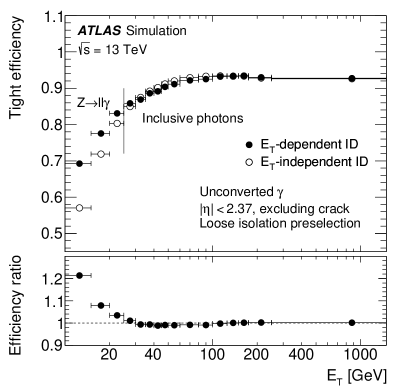
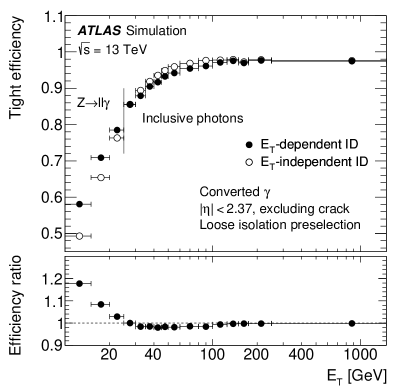
Figures 21 and 22 depict the Tight identification efficiencies for unconverted and converted photons as measured with the three efficiency methods. The data/MC scale factors are also shown for each measurement separately. The three efficiency measurements are performed using different processes, with different event topologies that may impact the photon efficiency. Despite this fact, the efficiency measurements are compatible within their statistical and systematic uncertainties.
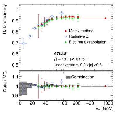
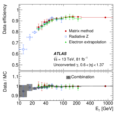
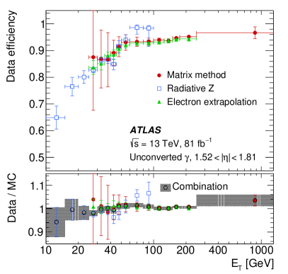
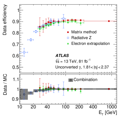
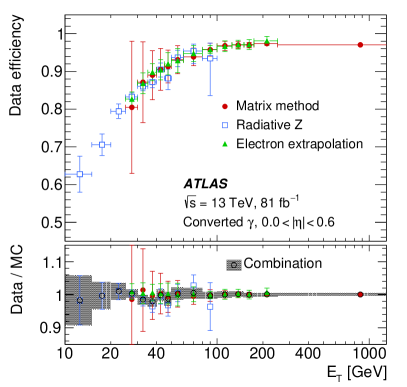
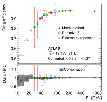
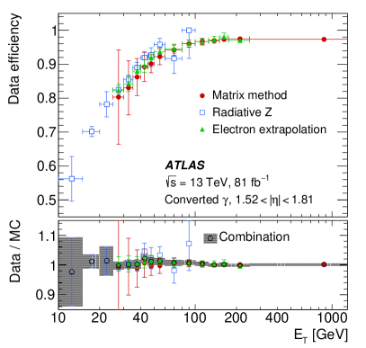
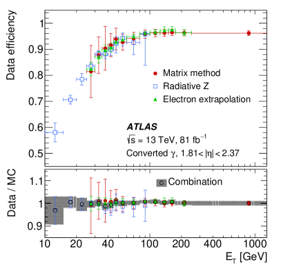
The scale factors from each of the three efficiency measurements are combined using a weighted average. The statistical and systematic uncertainties are assumed to be uncorrelated between the methods. The total uncertainty of the combined scale factors ranges between 7% at low and 0.5% at high for unconverted photons, and between 12% (low ) and less than 1% (high ) for converted photons. For > 1.5 TeV, where no measurement is performed, the scale factor measured in the bin [0.25,1.5] TeV is used, with the same uncertainty.
8 Electron and photon isolation
The activity near leptons and photons can be quantified from the tracks of nearby charged particles, or from energy deposits in the calorimeters, leading to two classes of isolation variables.
The raw calorimeter isolation [2] () is built by summing the transverse energy of positive-energy topological clusters whose barycentre falls within a cone centred around the electron or photon cluster barycentre. The topological cluster energy scale is the EM scale. The raw calorimeter isolation includes the EM particle energy (), which is subtracted by removing the energy of the EM calorimeter cells contained in a (in EM-middle-layer units) rectangular cluster around the barycentre of the EM particle cluster. The advantage of this simple method is a stable subtraction for real or fake/non-prompt objects for any transverse momentum and pile-up. The disadvantage is that it does not subtract all the EM particle energy and an additional leakage correction is needed. This leakage is parameterized as a function of and using MC samples of single electrons or photons without pile-up. Additionally, a correction for the pile-up and underlying-event contribution to the isolation cone is also estimated [39].
Finally, the fully corrected calorimeter isolation variable is computed as:
where refers to the size of the employed cone, . A cone size is used for the electron working points whereas cone sizes and 0.4 are used for photon working points.
The track isolation variable () is computed by summing the transverse momentum of selected tracks within a cone centred around the electron track or the photon cluster direction. Tracks matched to the electron or converted photon are excluded. Since for electrons produced in the decay of high-momentum heavy particles, other decay products can be very close to the electron direction, the track isolation for electrons is defined with a variable cone size () – the cone size shrinks for larger transverse momentum of the electron:
where is the maximum cone size (typically 0.2).
The tracks considered are required to have and , at least seven silicon (Pixel + SCT) hits, at most one shared hit (defined as , where and are the numbers of hits assigned to several tracks in the Pixel and SCT detectors), at most two silicon holes (i.e. missing hits in the pixel and SCT detectors) and at most one pixel hole. In addition, for electron isolation, the tracks are required to have a loose vertex association, i.e. the track was used in the primary vertex fit, or it was not used in any vertex fit but satisfies mm, where is the longitudinal impact parameter relative to the chosen primary vertex; for photon isolation, all selected tracks satisfying mm are used.
In this section, the isolation efficiency measurements are illustrated with the data recorded in 2017; nevertheless, the measurements are performed for the full high- dataset described in Section 3.1.
8.1 Electron isolation criteria and efficiency measurements
The implementation of isolation criteria is specific to the physics analysis needs, as it results from a compromise between a highly-efficient identification of prompt electrons, isolated or produced in a busy environment, and a good rejection of electrons from heavy-flavour decays or light hadrons misidentified as electrons. The different electron-isolation working points used in ATLAS are presented in Table 2.
The working points can be defined in two different ways, targeting a fixed value of efficiency or with fixed cuts on the isolation variables. The Gradient working point is designed to give an efficiency of 90% at and at , uniform in . The requirements on and (cut maps) for this working point are derived from () and () MC simulations and Tight identification requirements. The three other working points, HighPtCaloOnly, Loose and Tight, have a fixed requirement on the calorimeter and/or the track isolation variables.
| Working point | Calorimeter isolation | Track isolation |
|---|---|---|
| Gradient | (with ) | (with ) |
| HighPtCaloOnly | - | |
| Loose | ||
| Tight |
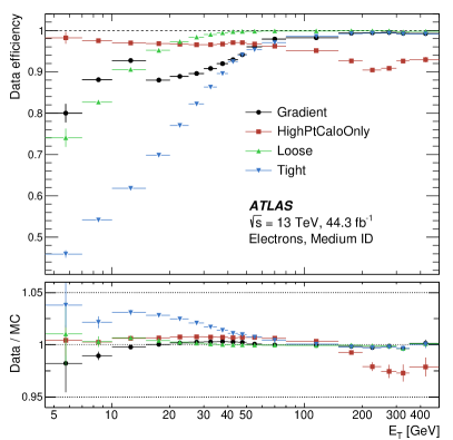
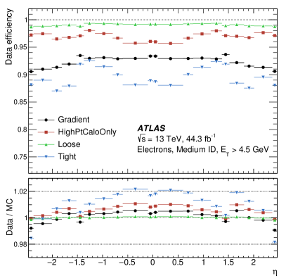
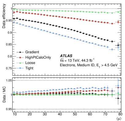
Figure 23 shows the electron isolation efficiency measured in data recorded in 2017 and the corresponding data-to-MC simulation ratios as a function of the electron and , and of the number of interactions per bunch crossing for the isolation working points summarized in Table 2. The pile-up correction to the calorimeter isolation is applied, and reduces the dependence of the isolation efficiency by about a factor of five. These results are obtained using a sample enriched in events, where the electrons satisfy the Medium identification. The method used to compute the electron isolation efficiency and the associated uncertainties are described in Ref. [2]. For Gradient, a jump in the efficiency is observed at the transition point of 15 GeV because the value of the isolation efficiency is process dependent: the cut maps are optimized with events below 15 GeV, while the measurement is performed with events in the full range. The Tight operating point gives the highest background rejection below 60 GeV and the most significant difference in shape in . As the name suggests, HighPtCaloOnly gives the highest rejection in the high- region (). The Gradient and Tight operating points give the highest pile-up dependency, the isolation efficiency decreasing from 95% at low to 85% when is around 70–80.
The overall differences between data and MC simulation are less than approximately 1–5% depending on the working point, with the largest difference observed for Tight isolation. For electrons with higher than no measurement can be performed because of the limited number of data events, and the results from the bin [300,500] GeV are used with an additional systematic uncertainty varying betwen 0.1% and 1.7%, depending on the isolation working point. The overall scale factor uncertainties range from about 5% for electrons with below 7 GeV, to less than 0.5% towards high .
8.2 Photon isolation criteria and efficiency measurements
| Working point | Calorimeter isolation | Track isolation |
|---|---|---|
| Loose | ||
| Tight | GeV | |
| TightCaloOnly | GeV | - |
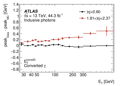
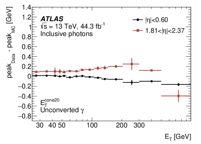
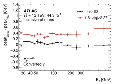
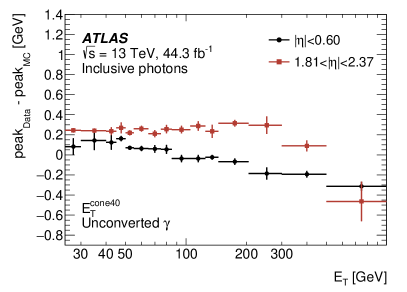

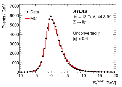
Three photon isolation operating points are defined using requirements on the calorimeter and track isolation variables, as summarized in Table 3. For the calorimeter-based photon isolation variables a discrepancy between the peak positions of their distributions in data and simulation has been observed since Run 1 [40], pointing to a mismodelling in simulation of the lateral profile development of the electromagnetic showers. As a result, the photon isolation efficiencies in data and simulations disagree, leading to scale factors significantly different from 1.
These discrepancies are mitigated by applying data-driven shifts to the calorimeter isolation variables for photons in simulation. The shifts are obtained by performing fits to the calorimeter isolation variable distribution, using Crystal Ball pdfs [41], in regions dominated by real photons, in data and simulation. The fits are performed in bins of photon , and conversion status, separately for and isolation variables. The difference in the fitted peak values between data and simulation defines the shift value, which is added to the photon calorimeter isolation values in simulation. Figure 24 illustrates the data-driven shifts obtained with 2017 data and the Pythia8 simulation for the and isolation variables in two regions. Figure 25 shows the distribution of the isolation variable in 2017 data and simulation, using events after the data-driven shifts are applied.
The photon isolation efficiency is studied in two main signatures: radiative decays (valid for ) and inclusive photons (used in the 1.5 TeV range).
8.2.1 Measurement of photon isolation efficiency with radiative decays
As detailed in Section 7, final-state radiation in -boson decays provides a clean environment to probe photons in the low- range. Using the same method as for the photon identification, photon isolation efficiencies are measured for the operating points presented in Table 3. The evolution of the isolation efficiency measured in 2017 data as a function of and is illustrated in Figure 26, together with the data-to-simulation efficiency ratio. The overall differences between data and simulation are less than approximately 5%. The decrease of efficiency with increasing pile-up activity is shown in Figure 27. A loss of efficiency of 10% is measured when increasing from 15 to 60. This loss is well described by the simulation.
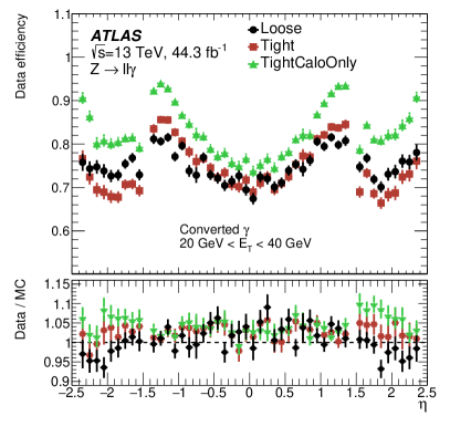

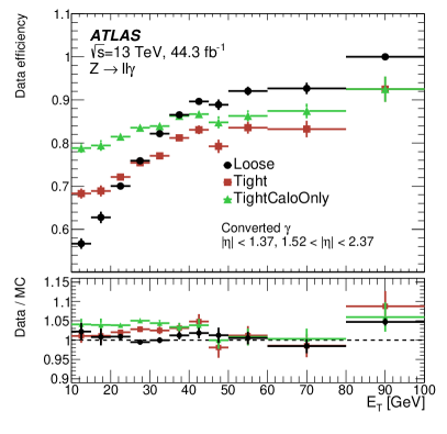
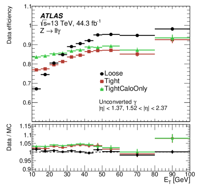
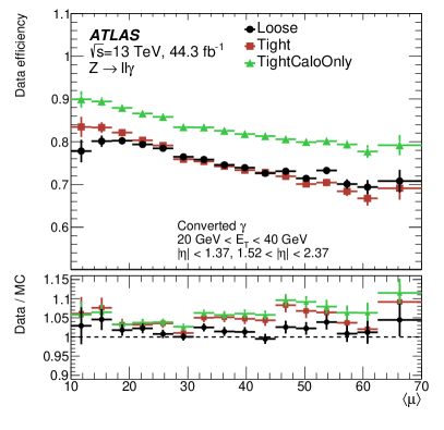
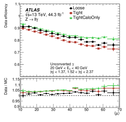
8.2.2 Photon calorimeter isolation efficiency measurement with inclusive-photon events
Photon isolation studies with inclusive-photon events are performed using two different methods for the calorimeter-based and track-based isolations. This is because the distribution of the track isolation variable shows a large peak at followed by a 1 GeV gap, due to the selection of the tracks entering the computation, and by a small tail, and cannot be fitted with an analytic function. In consequence, the efficiency measurement is done separately for the track isolation and calorimeter isolation criteria applied to define the working points presented in Table 3. When the measurement is performed for the track-based (calorimeter-based) isolation, the requirements on the calorimeter-based (track-based) isolation are applied at preselection level to reduce the background from jets.
The photon calorimeter isolation (calo-only) efficiency with inclusive-photon events is obtained by fitting the distribution of the calorimeter isolation, or , minus the relevant fraction ( for Tight and for Loose), hereafter simply called the isolation distribution. The measurement is performed in bins of photon , , conversion status and data-taking period. The Pythia8 inclusive-photon sample described in Section 3.2 is used for the true photon template.
A set of alternate selections is used to determine the isolation distributions for the backgound and their uncertainty. These criteria, denoted LoosePrime, select photon candidates that pass the Loose identification but fail at least one out of shower shape cuts used in the Tight identification. 999The sets of criteria of which at least one is not satisfied are requirements on {, } for =2; {, , } for =3; {, , , } for =4 and {, , , , } for =5. The nominal background template is obtained from photon candidates passing the LoosePrime4 identification. As in the measurements of the data-driven shifts, the photon isolation efficiency is obtained by performing a set of fits in regions defined in simulation and data. Although background enriched, the sample passing LoosePrime4 also contains true photons that fail the Tight identification requirement; these are defined as ‘leakage’ photons and subtracted. The sequence of fits proceeds as follows:
-
1.
A model for the isolation distribution for signal photons is defined from a fit, using a Crystal Ball function, to the isolation distribution obtained for tightly identified photons in simulation.
-
2.
The corresponding model for leakage photons is defined from a fit to the isolation distribution obtained for LoosePrime4 photons in simulation.
-
3.
The isolation distribution for background photons (i.e. the sum of fake and leakage photons) is parameterized using a two-component fit to the distribution observed for photons satisfying the LoosePrime4 requirement in data. An unconstrained Crystal Ball function is used to model the isolation distribution for fake photons, and the model for leakage photons is defined in point 2.
-
4.
Finally, the number of signal photons is estimated from a two-component fit to the isolation distribution observed for tightly identified photons in data. The background component uses the model defined in point 3, and the signal photon component uses the model defined in point 1.
The fits described in points 3 and 4 above are performed twice. The first time, they are performed to estimate the number of leakage photons from the ratio of the number of photon candidates passing the Tight and LoosePrime4 identification selection. When the fit in the LoosePrime4 sample is performed again (point 3), the number of leakage photons is constrained, allowing a better estimation of the fake photon isolation distribution. Finally the fit in the tightly identified sample is also redone, with the background component formed only by fake photons. Once the background component is subtracted, only real photons meeting the Tight identification criterion remain and are used for the isolation efficiency measurements.
Finally, the calo-only isolation efficiency in data is obtained by integrating the background-subtracted isolation distribution for tightly identified photons in data, up to the working point cut-off of 0 GeV (Loose) or 2.45 GeV (Tight and TightCaloOnly). Three sources of systematic uncertainty are considered: discrepancies between the fitted isolation distribution and that observed for photons in data; differences between results obtained using LoosePrime3 and LoosePrime5 instead of LoosePrime4 for the determination of the background templates; and uncertainties in the estimation of the number of leakage photons in the LoosePrime4 sample. A binomial statistical error in the scale factors is also calculated and added in quadrature to the systematic components.
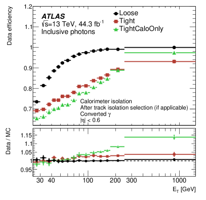
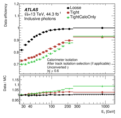
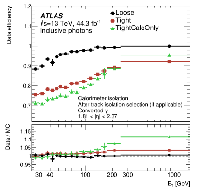
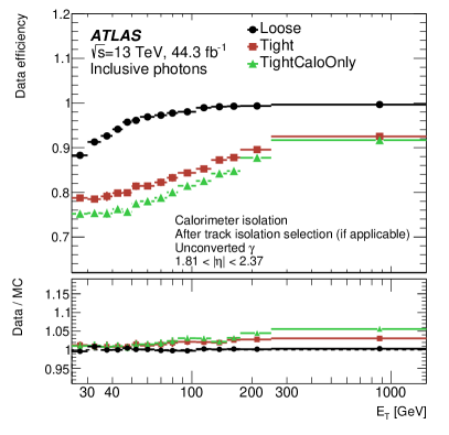
The calo-only isolation efficiencies measured with inclusive-photon events in 2017 data are shown in Figure 28. The overall differences between data and simulation increase from a few percent in the low region up to 15% at high ( GeV) for the TightCaloOnly working point, and only up to 5% for Loose and Tight.
8.2.3 Photon track-based isolation efficiency measurement with inclusive-photon events
As in the measurement of the calo-only photon isolation efficiency, the main source of background comes from jets misidentified as photons. This background is estimated with a template fit to the track isolation distribution, in a region enriched in background photons satisfying LoosePrime4 but failing the Tight identification criterion. The track-only photon isolation efficiency is measured in a signal region enriched in tightly identified photons, after the background is subtracted. To assign the systematic uncertainties, the fit range is varied as well as the definition of the background template, where the photons are required to pass LoosePrime2, LoosePrime3 or LoosePrime5 instead of the LoosePrime4 criterion. Efficiencies for each configuration are computed, and with them the corresponding scale factors. Once the different scale factors are calculated, a bin-by-bin scan is performed, keeping the largest deviation from the nominal value among the considered variations. The total uncertainty is obtained by adding the systematic and statistical components in quadrature.
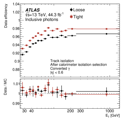
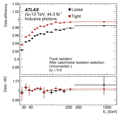
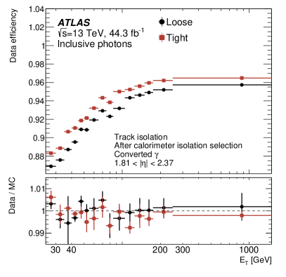
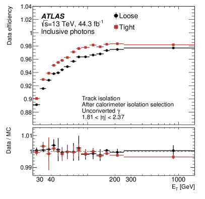
The track-only isolation efficiencies measured with inclusive-photon events in 2017 data are shown in Figure 29. The ratio of the data to MC simulation is close to unity.
8.2.4 Combination of photon isolation scale factors
The photon isolation scale factors are measured for the three isolation working points detailed in Table 3 using radiative decays and inclusive-photon events. The different results are combined to obtain one set of scale factors per working point, data-taking year, and photon conversion status. The combination is performed in two steps. First, the track-only and calo-only scale factors determined with inclusive-photon events are multiplied together to obtain a single set per configuration. These inclusive-photon scale factors are further combined with those determined with radiative decay events using a simple weighted average. The uncertainties in the track-only and calo-only results obtained with inclusive-photon events are treated as fully correlated in the combination, while the uncertainties in the radiative- and inclusive-photon measurement results are treated as uncorrelated. The combination is performed for GeV; below 25 GeV, only results from radiative decays are available, while above 100 GeV the results are obtained with inclusive-photon events only. If, in a given (, ) bin, the total uncertainty in the combined scale factor does not cover the difference between the values obtained from the two samples, it is scaled such that . Above , the results obtained in the last bin used for the measurement are considered, with no change in the systematic uncertainty.
For < 25 GeV, the measurements achieve a typical uncertainty of about 2%, and at worst 5–10% for < 15 GeV. For > 100 GeV, uncertainties around 1–2% are obtained. For GeV, the combination of the two channels reduces the scale factor uncertainties to about 1% on average.
9 Electron charge misidentification
The reconstruction of the electric charge of an electron relies solely on the measurement of the curvature of its associated track in the inner detector. Interactions of an electron with the detector material can create secondary particles: photons and electron–positron pairs. The production of these secondary particles can lead to distortions of the primary electron track, e.g. hits from the secondary particle being included in the fit of the primary electron track, and the presence of additional tracks of secondary particles in the vicinity of the primary electron track. Incorrect charge reconstruction can thus be caused either by an incorrect determination of the track curvature, or by the choice of an incorrect track.
For electrons at high transverse momentum, the first effect becomes dominant and leads to an almost linear increase with energy in the probability to determine the sign of the curvature incorrectly. Final-state radiation emitted collinearly off the electron can also cause charge misidentification if the radiated photon subsequently converts to an electron–positron pair in the detector material. Here, the correct or incorrect charge is assigned with equal probability. The electric charge is heavily used as a selection criterion in measurements with the ATLAS experiment, and hence understanding the effects of charge misidentification is important. Some specific signatures also require the suppression of electron charge misidentification in order to reduce background.
9.1 Suppression of electron charge misidentification
The suppression of electron charge misidentification is based on the output discriminant of a boosted decision tree (BDT). A previous version, optimized for data recorded in 2015 and 2016, rejected 90% of electrons with incorrectly reconstructed charge, removing only 3% of electrons with correctly reconstructed charge [2]. The optimization was based on simulated electrons and showed a higher rejection than observed in data. In the following, a re-optimization of the BDT is described. Data from decays are used to reduce efficiency losses due to mismodelling of the input variables in the BDT training. Furthermore, additional input variables have been studied.
To select a relatively clean sample of electrons with correctly and incorrectly reconstructed charge, one of the electrons is restricted to , required to satisfy Tight identification and to pass the 97% operating point of the previous BDT discriminant. These requirements minimize charge misidentification for this electron. Any additional reconstructed electron in the event is used to train the BDT, as a signal electron if it has an electric charge different from the first electron, and as a background electron if the electric charge is the same. To reduce background from converted photons from initial- or final-state radiation, the invariant mass of any pairs of electrons must lie within 5 GeV of 90 GeV in opposite-charge events and within 5 GeV of 88 GeV in same-charge events. The lower value used in same-charge events accounts for the fact that electrons with the incorrect charge have a higher probability for energy loss as discussed in Section 9.2 and illustrated in Figure 30(a).
Input quantities to the BDT are the electron and , and a set of additional variables. In decreasing order of separation power, these are: the transverse impact parameter multiplied by the electron electric charge , the average charge of all tracks matched to the electron weighted by their number of hits in the SCT detector , and . With the BDT includes for the first time the reconstructed properties of additional tracks in the vicinity of the electron, which improves rejection in cases where the incorrect track is chosen as the primary electron track.
The efficiency of the requirement on the BDT is 98% in events for electrons satisfying Medium or Tight identification with the Tight isolation requirement, and that have the correct electric charge. Approximately 90% of electrons with the same identification and isolation requirements but incorrect electric charge are removed. This re-optimization of the BDT variables has improved the efficiency of the selection criterion, leaving the rejection of electrons with misidentified charge unchanged.
9.2 Measurement of the probability for charge misidentification
The probability for electron charge misidentification is measured in seven bins in and six bins in the range in events. The events were collected with the dielectron triggers discussed in Section 3.1 with transverse momentum thresholds of 17 GeV or less and Loose trigger identification, allowing the measurement to be extended to lower values of and looser identification criteria than previous measurements. Both electrons in the event are selected with the same identification and isolation criteria and, respectively, fall into bins and in , yielding events. Their invariant mass must lie within 10 GeV of the nominal -boson mass. The probabilities of the electron charge misidentification in bins and , and , maximize the Poisson probability , where:
and is the number of same-charge events. The number of background events in the sample where both electrons have the same electric charge, , consists of misidentified electrons from multijet production and electrons from converted photons from the aforementioned final-state radiation. The two components are estimated in a sideband subtraction and from simulation, respectively. The selected data and the estimated background is shown in Figure 30(a) for an example bin. Sources of systematic uncertainties in the measurement are the estimation of the background from multijet production and final-state radiation, and the restriction of the dielectron invariant mass. Possible biases in the experimental method used to perform the measurement are evaluated by comparing the charge misidentification probability obtained in the likelihood maximization in simulation with those obtained using generator-level information.
The kinematic range of GeV is particularly relevant for searches for physics beyond the Standard Model with same-charge signatures. For a measurement with high granularity, the double differential charge misidentification probabilities are factorized into an - and an -dependent part. This approach allows measurements in 5 bins in and 14 bins in with reasonable statistical precision from a sample of approximately 9000 electrons with the incorrect charge assignment (for Tight identification). The systematic uncertainty in the parameterization is assessed by comparing, double differentially, the ratio of same-charge events and opposite-charge events, weighted with the charge misreconstruction probability, in data and simulation. The systematic uncertainty is derived by incrementing the uncertainty in steps of 1% until the value falls below 1, separately in each bin in .
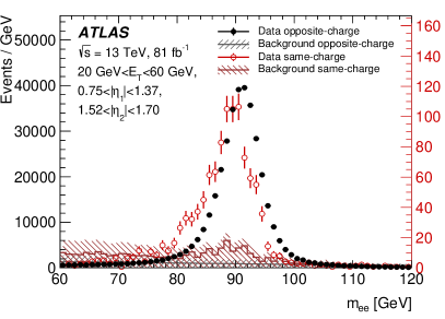
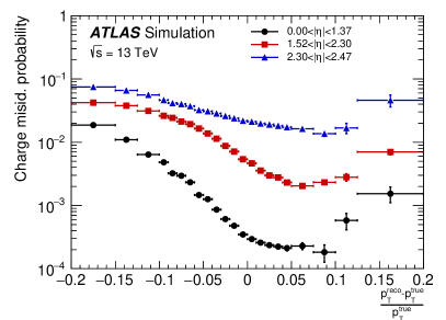
The interactions with material in the inner detector causing electron charge misidentification can also lead to significant energy loss and leakage of energy outside the EM cluster, introducing a correlation between the two effects. In Figure 30(b), the charge misidentification probability is shown as a function of the energy response, , in several bins of . It increases with the difference between true and reconstructed electron energy. The same effect causes the differences in reconstructed invariant mass between opposite-charge and same-charge events shown in Figure 30(a). The correlation with the energy response complicates the measurement of charge misidentification probabilities in data. The probability measurement is blind as to which of the two electrons has the incorrect charge assignment. Hence, the probabilities determined from the likelihood maximization are used to form data-to-simulation probability ratios. No significant dependence of the data-to-simulation ratios on the dilepton invariant mass has been observed. The charge misidentification probabilities in data are obtained by multiplying the data-to-simulation probability ratios by the charge misidentification probabilities computed in the simulation, where the electron with the incorrect charge assignment is unambiguous. The probabilities in data are shown in Figure 31 for several combinations of identification and isolation operating points. For Medium identification with Tight isolation, the electron charge misidentification probability in events is smallest in the central region of the detector at 0.05%, and increases to 2.7% at high . As a function of it increases approximately linearly from 0.28% at GeV to 1.7% at GeV. With Tight instead of Medium identification, a reduction of charge misidentification by 25%–50%, depending on and , is seen. The BDT presented in Section 9.1 further reduces the misidentification probability by factor of about five, on average over the detector acceptance, and by up to a factor 10 at high pseudorapidity.
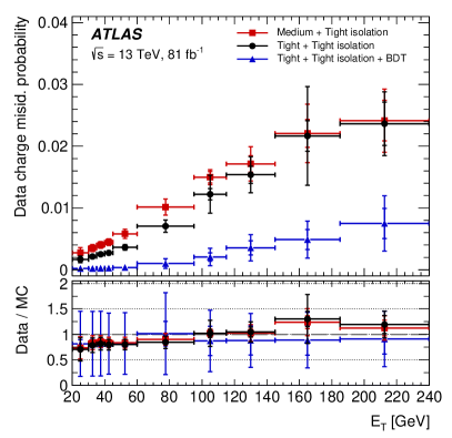
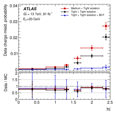
10 Conclusions
The reconstruction of electrons and photons based on a dynamical, topological cell clustering algorithm has been described, and the corresponding updates to the methods used for the identification of the candidates and the estimation of their energy have been discussed. The rejection of non-isolated particles and of mismeasured electron candidates have been re-optimized accordingly.
The dynamical cell clustering algorithm provides an electron and photon reconstruction efficiency similar to that of the sliding-window reconstruction. A relative improvement of about 15% is obtained in the reconstruction efficiency for two-track photon conversions. The misclassification of unconverted photons as single-track TRT conversions is reduced by a factor of two, while the single-track conversion reconstruction efficiency only decreases by 5 to 10%. The present algorithm also provides a better energy measurement, with a relative improvement in resolution by about 15% in the barrel, and about 20–25% in the endcap, for electrons and converted photons. The resolution for unconverted photons is unchanged.
Energy scale and resolution corrections have been measured using electrons from decays. A significant dependence of the corrections on the amount of pile-up has been observed, reflecting a mismodelling of the calorimeter activity in minimum-bias events. The uncertainty in the energy scale corrections ranges from in the barrel to in the endcap. The uncertainty in the constant-term resolution corrections is typically 1–. The electron-based energy calibration has been verified for photons, using radiative -boson decays, to a precision of 0.5% at worst.
The identification of electrons and photons has been revisited to match the improved cell clustering procedure. For electrons, identification efficiencies vary from 93% for the Loose identification criterion, to 80% for the Tight criterion, for electrons from -boson decays. The simulation models these efficiencies to a precision of 2% for Loose electrons and 5% for Tight electrons, respectively. The efficiency correction factors are measured with a typical precision of 0.2%. In the case of photons, the identification efficiency reaches 92% for unconverted photons, and 98% for converted photons, for GeV and above. The precision of the efficiency correction factors ranges from 7% at low to 0.5% at high for unconverted photons, and from 12% to 1% for converted photons.
Several electron and photon isolation selection criteria have been defined, targeting a range of processes with varying event activity. The efficiencies of the isolation selections vary from about 99% for the loosest, to about 90% for the tightest criterion, depending on the physics process. Tight isolation selections exhibit a steeply rising efficiency as a function of ; for all isolation criteria, the selection efficiency varies by about 10% as a function of , for the range of spanned by the present dataset. Differences in efficiency between data and simulation range from 1% to 5%, depending on and .
A dedicated algorithm has been implemented to reject electrons with badly measured track parameters, with the main objective of reducing the fraction of electron candidates with wrongly measured charge. This fraction, rising from less than 0.1% in the barrel to about 3% at high for all candidates, is reduced by a factor of three to five as a function of , and by up to a factor of ten at high . The simulation is found to model the data within 20% for the residual fraction of wrong-charge electron candidates, and the corresponding correction factors are measured with about 50% precision.
The present results define the baseline performance of the ATLAS detector for searches and measurements using electrons and photons from LHC proton–proton collision data collected at TeV.
Acknowledgements
We thank CERN for the very successful operation of the LHC, as well as the support staff from our institutions without whom ATLAS could not be operated efficiently.
We acknowledge the support of ANPCyT, Argentina; YerPhI, Armenia; ARC, Australia; BMWFW and FWF, Austria; ANAS, Azerbaijan; SSTC, Belarus; CNPq and FAPESP, Brazil; NSERC, NRC and CFI, Canada; CERN; CONICYT, Chile; CAS, MOST and NSFC, China; COLCIENCIAS, Colombia; MSMT CR, MPO CR and VSC CR, Czech Republic; DNRF and DNSRC, Denmark; IN2P3-CNRS, CEA-DRF/IRFU, France; SRNSFG, Georgia; BMBF, HGF, and MPG, Germany; GSRT, Greece; RGC, Hong Kong SAR, China; ISF and Benoziyo Center, Israel; INFN, Italy; MEXT and JSPS, Japan; CNRST, Morocco; NWO, Netherlands; RCN, Norway; MNiSW and NCN, Poland; FCT, Portugal; MNE/IFA, Romania; MES of Russia and NRC KI, Russian Federation; JINR; MESTD, Serbia; MSSR, Slovakia; ARRS and MIZŠ, Slovenia; DST/NRF, South Africa; MINECO, Spain; SRC and Wallenberg Foundation, Sweden; SERI, SNSF and Cantons of Bern and Geneva, Switzerland; MOST, Taiwan; TAEK, Turkey; STFC, United Kingdom; DOE and NSF, United States of America. In addition, individual groups and members have received support from BCKDF, CANARIE, CRC and Compute Canada, Canada; COST, ERC, ERDF, Horizon 2020, and Marie Skłodowska-Curie Actions, European Union; Investissements d’ Avenir Labex and Idex, ANR, France; DFG and AvH Foundation, Germany; Herakleitos, Thales and Aristeia programmes co-financed by EU-ESF and the Greek NSRF, Greece; BSF-NSF and GIF, Israel; CERCA Programme Generalitat de Catalunya, Spain; The Royal Society and Leverhulme Trust, United Kingdom.
The crucial computing support from all WLCG partners is acknowledged gratefully, in particular from CERN, the ATLAS Tier-1 facilities at TRIUMF (Canada), NDGF (Denmark, Norway, Sweden), CC-IN2P3 (France), KIT/GridKA (Germany), INFN-CNAF (Italy), NL-T1 (Netherlands), PIC (Spain), ASGC (Taiwan), RAL (UK) and BNL (USA), the Tier-2 facilities worldwide and large non-WLCG resource providers. Major contributors of computing resources are listed in Ref. [42].
References
- [1] ATLAS Collaboration “Measurement of the photon identification efficiencies with the ATLAS detector using LHC Run 2 data collected in 2015 and 2016” In Eur. Phys. J. C 79, 2019, pp. 205 DOI: 10.1140/epjc/s10052-019-6650-6
- [2] ATLAS Collaboration “Electron reconstruction and identification in the ATLAS experiment using the 2015 and 2016 LHC proton–proton collision data at = ” In Eur. Phys. J. C 79, 2019, pp. 639 DOI: 10.1140/epjc/s10052-019-7140-6
- [3] ATLAS Collaboration “Electron and photon energy calibration with the ATLAS detector using 2015–2016 LHC proton–proton collision data” In JINST 14, 2019, pp. P03017 DOI: 10.1088/1748-0221/14/03/P03017
- [4] ATLAS Collaboration “Topological cell clustering in the ATLAS calorimeters and its performance in LHC Run 1” In Eur. Phys. J. C 77, 2017, pp. 490 DOI: 10.1140/epjc/s10052-017-5004-5
- [5] ATLAS Collaboration “The ATLAS Experiment at the CERN Large Hadron Collider” In JINST 3, 2008, pp. S08003 DOI: 10.1088/1748-0221/3/08/S08003
- [6] ATLAS Collaboration “ATLAS Insertable B-Layer Technical Design Report”, ATLAS-TDR-19, 2010 URL: https://cds.cern.ch/record/1291633
- [7] B. Abbott “Production and integration of the ATLAS Insertable B-Layer” In JINST 13, 2018, pp. T05008 DOI: 10.1088/1748-0221/13/05/T05008
- [8] ATLAS Collaboration “Performance of the ATLAS trigger system in 2015” In Eur. Phys. J. C 77, 2017, pp. 317 DOI: 10.1140/epjc/s10052-017-4852-3
- [9] ATLAS Collaboration “Muon reconstruction performance of the ATLAS detector in proton–proton collision data at ” In Eur. Phys. J. C 76, 2016, pp. 292 DOI: 10.1140/epjc/s10052-016-4120-y
- [10] Simone Alioli, Paolo Nason, Carlo Oleari and Emanuele Re “NLO vector-boson production matched with shower in POWHEG” In JHEP 07, 2008, pp. 060 DOI: 10.1088/1126-6708/2008/07/060
- [11] Torbjorn Sjöstrand, Stephen Mrenna and Peter Z. Skands “A brief introduction to PYTHIA 8.1” In Comput. Phys. Commun. 178, 2008, pp. 852–867 DOI: 10.1016/j.cpc.2008.01.036
- [12] Hung-Liang Lai et al. “New parton distributions for collider physics” In Phys. Rev. D 82, 2010, pp. 074024 DOI: 10.1103/PhysRevD.82.074024
- [13] ATLAS Collaboration “Measurement of the boson transverse momentum distribution in collisions at with the ATLAS detector” In JHEP 09, 2014, pp. 145 DOI: 10.1007/JHEP09(2014)145
- [14] J. Pumplin et al. “New generation of parton distributions with uncertainties from global QCD analysis” In JHEP 07, 2002, pp. 012 DOI: 10.1088/1126-6708/2002/07/012
- [15] N. Davidson, T. Przedzinski and Z. Was “PHOTOS interface in C++: Technical and physics documentation” In Comput. Phys. Commun. 199, 2016, pp. 86–101 DOI: 10.1016/j.cpc.2015.09.013
- [16] T. Gleisberg et al. “Event generation with Sherpa 1.1” In JHEP 02, 2009, pp. 007 DOI: 10.1088/1126-6708/2009/02/007
- [17] Richard D. Ball “Parton distributions for the LHC Run II” In JHEP 04, 2015, pp. 040 DOI: 10.1007/JHEP04(2015)040
- [18] ATLAS Collaboration “ATLAS Pythia 8 tunes to data”, ATL-PHYS-PUB-2014-021, 2014 URL: https://cds.cern.ch/record/1966419
- [19] Richard D. Ball “Parton distributions with LHC data” In Nucl. Phys. B 867, 2013, pp. 244–289 DOI: 10.1016/j.nuclphysb.2012.10.003
- [20] D.. Lange “The EvtGen particle decay simulation package” In Proceedings, 7th International Conference on B physics at hadron machines (BEAUTY 2000): Maagan, Israel, September 13-18, 2000 462, 2001, pp. 152–155 DOI: 10.1016/S0168-9002(01)00089-4
- [21] ATLAS Collaboration “The ATLAS Simulation Infrastructure” In Eur. Phys. J. C 70, 2010, pp. 823 DOI: 10.1140/epjc/s10052-010-1429-9
- [22] S. Agostinelli “Geant4 – a simulation toolkit” In Nucl. Instrum. Meth. A 506, 2003, pp. 250–303 DOI: 10.1016/S0168-9002(03)01368-8
- [23] ATLAS Collaboration “The Pythia 8 A3 tune description of ATLAS minimum bias and inelastic measurements incorporating the Donnachie–Landshoff diffractive model”, ATL-PHYS-PUB-2016-017, 2016 URL: https://cds.cern.ch/record/2206965
- [24] ATLAS Collaboration “Summary of ATLAS Pythia 8 tunes”, ATL-PHYS-PUB-2012-003, 2012 URL: https://cds.cern.ch/record/1474107
- [25] ATLAS Collaboration “Performance of the ATLAS track reconstruction algorithms in dense environments in LHC Run 2” In Eur. Phys. J. C 77, 2017, pp. 673 DOI: 10.1140/epjc/s10052-017-5225-7
- [26] Walter Lampl “Calorimeter Clustering Algorithms: Description and Performance”, ATL-LARG-PUB-2008-002, 2008 URL: https://cds.cern.ch/record/1099735
- [27] Thijs G. Cornelissen “Concepts, design and implementation of the ATLAS New Tracking (NEWT)”, ATL-SOFT-PUB-2007-007, 2007 URL: https://cds.cern.ch/record/1020106
- [28] R. Frühwirth “Application of Kalman filtering to track and vertex fitting” In Nucl. Instrum. Meth. A 262, 1987, pp. 444–450 DOI: 10.1016/0168-9002(87)90887-4
- [29] Thijs G. Cornelissen et al. “The global track fitter in ATLAS” In Proceedings, 16th International Conference on Computing in High Energy and Nuclear Physics (CHEP 2007): Victoria, Canada, September 2-7, 2007 119, 2008, pp. 032013 DOI: 10.1088/1742-6596/119/3/032013
- [30] ATLAS Collaboration “Improved electron reconstruction in ATLAS using the Gaussian Sum Filter-based model for bremsstrahlung”, ATLAS-CONF-2012-047, 2012 URL: https://cds.cern.ch/record/1449796
- [31] ATLAS Collaboration “Particle Identification Performance of the ATLAS Transition Radiation Tracker”, ATLAS-CONF-2011-128, 2011 URL: https://cds.cern.ch/record/1383793
- [32] ATLAS Collaboration “Performance of the ATLAS Transition Radiation Tracker in Run 1 of the LHC: tracker properties” In JINST 12, 2017, pp. P05002 DOI: 10.1088/1748-0221/12/05/P05002
- [33] C La Taille and L Serin “Temperature dependance of the ATLAS electromagnetic calorimeter signal. Preliminary drift time measurement”, ATL-LARG-95-029, 1995 URL: https://cds.cern.ch/record/686091
- [34] ATLAS Collaboration “Study of the material of the ATLAS inner detector for Run 2 of the LHC” In JINST 12, 2017, pp. P12009 DOI: 10.1088/1748-0221/12/12/P12009
- [35] David W. Scott “Multivariate Density Estimation, Theory, Practice, and Visualization” Wiley- Interscience, New York, 1992
- [36] Andreas Hoecker “TMVA: Toolkit for Multivariate Data Analysis”, 2007 arXiv:physics/0703039 [physics.data-an]
- [37] ATLAS Collaboration “Electron efficiency measurements with the ATLAS detector using 2012 LHC proton–proton collision data” In Eur. Phys. J. C 77, 2017, pp. 195 DOI: 10.1140/epjc/s10052-017-4756-2
- [38] Luc Devroye “Non-Uniform Random Variate Generation” Springer-Verlag, 1986
- [39] Matteo Cacciari and Gavin P. Salam “Pileup subtraction using jet areas” In Phys. Lett. B 659, 2008, pp. 119–126 DOI: 10.1016/j.physletb.2007.09.077
- [40] ATLAS Collaboration “Electron performance measurements with the ATLAS detector using the 2010 LHC proton–proton collision data” In Eur. Phys. J. C 72, 2012, pp. 1909 DOI: 10.1140/epjc/s10052-012-1909-1
- [41] M. Oreglia “A Study of the Reactions ”, 1980 URL: https://www-public.slac.stanford.edu/sciDoc/docMeta.aspx?slacPubNumber=slac-r-236
- [42] ATLAS Collaboration “ATLAS Computing Acknowledgements”, ATL-GEN-PUB-2016-002 URL: https://cds.cern.ch/record/2202407
- [43] ATLAS Collaboration, ATLAS-TDR-19-ADD-1, 2012 URL: https://cds.cern.ch/record/1451888
The ATLAS Collaboration
G. Aad, B. Abbott, D.C. Abbott, A. Abed Abud, K. Abeling, D.K. Abhayasinghe, S.H. Abidi, O.S. AbouZeid, N.L. Abraham, H. Abramowicz, H. Abreu, Y. Abulaiti, B.S. Acharya, B. Achkar, S. Adachi, L. Adam, C. Adam Bourdarios, L. Adamczyk, L. Adamek, J. Adelman, M. Adersberger, A. Adiguzel, S. Adorni, T. Adye, A.A. Affolder, Y. Afik, C. Agapopoulou, M.N. Agaras, A. Aggarwal, C. Agheorghiesei, J.A. Aguilar-Saavedra, F. Ahmadov, W.S. Ahmed, X. Ai, G. Aielli, S. Akatsuka, T.P.A. Åkesson, E. Akilli, A.V. Akimov, K. Al Khoury, G.L. Alberghi, J. Albert, M.J. Alconada Verzini, S. Alderweireldt, M. Aleksa, I.N. Aleksandrov, C. Alexa, D. Alexandre, T. Alexopoulos, A. Alfonsi, F. Alfonsi, M. Alhroob, B. Ali, G. Alimonti, J. Alison, S.P. Alkire, C. Allaire, B.M.M. Allbrooke, B.W. Allen, P.P. Allport, A. Aloisio, A. Alonso, F. Alonso, C. Alpigiani, A.A. Alshehri, M. Alvarez Estevez, D. Álvarez Piqueras, M.G. Alviggi, Y. Amaral Coutinho, A. Ambler, L. Ambroz, C. Amelung, D. Amidei, S.P. Amor Dos Santos, S. Amoroso, C.S. Amrouche, F. An, C. Anastopoulos, N. Andari, T. Andeen, C.F. Anders, J.K. Anders, A. Andreazza, V. Andrei, C.R. Anelli, S. Angelidakis, A. Angerami, A.V. Anisenkov, A. Annovi, C. Antel, M.T. Anthony, M. Antonelli, D.J.A. Antrim, F. Anulli, M. Aoki, J.A. Aparisi Pozo, L. Aperio Bella, G. Arabidze, J.P. Araque, V. Araujo Ferraz, R. Araujo Pereira, C. Arcangeletti, A.T.H. Arce, F.A. Arduh, J-F. Arguin, S. Argyropoulos, J.-H. Arling, A.J. Armbruster, A. Armstrong, O. Arnaez, H. Arnold, Z.P. Arrubarrena Tame, A. Artamonov, G. Artoni, S. Artz, S. Asai, N. Asbah, E.M. Asimakopoulou, L. Asquith, J. Assahsah, K. Assamagan, R. Astalos, R.J. Atkin, M. Atkinson, N.B. Atlay, H. Atmani, K. Augsten, G. Avolio, R. Avramidou, M.K. Ayoub, A.M. Azoulay, G. Azuelos, H. Bachacou, K. Bachas, M. Backes, F. Backman, P. Bagnaia, M. Bahmani, H. Bahrasemani, A.J. Bailey, V.R. Bailey, J.T. Baines, M. Bajic, C. Bakalis, O.K. Baker, P.J. Bakker, D. Bakshi Gupta, S. Balaji, E.M. Baldin, P. Balek, F. Balli, W.K. Balunas, J. Balz, E. Banas, A. Bandyopadhyay, Sw. Banerjee, A.A.E. Bannoura, L. Barak, W.M. Barbe, E.L. Barberio, D. Barberis, M. Barbero, G. Barbour, T. Barillari, M-S. Barisits, J. Barkeloo, T. Barklow, R. Barnea, S.L. Barnes, B.M. Barnett, R.M. Barnett, Z. Barnovska-Blenessy, A. Baroncelli, G. Barone, A.J. Barr, L. Barranco Navarro, F. Barreiro, J. Barreiro Guimarães da Costa, S. Barsov, R. Bartoldus, G. Bartolini, A.E. Barton, P. Bartos, A. Basalaev, A. Bassalat, M.J. Basso, R.L. Bates, S. Batlamous, J.R. Batley, B. Batool, M. Battaglia, M. Bauce, F. Bauer, K.T. Bauer, H.S. Bawa, J.B. Beacham, T. Beau, P.H. Beauchemin, F. Becherer, P. Bechtle, H.C. Beck, H.P. Beck, K. Becker, M. Becker, C. Becot, A. Beddall, A.J. Beddall, V.A. Bednyakov, M. Bedognetti, C.P. Bee, T.A. Beermann, M. Begalli, M. Begel, A. Behera, J.K. Behr, F. Beisiegel, A.S. Bell, G. Bella, L. Bellagamba, A. Bellerive, P. Bellos, K. Beloborodov, K. Belotskiy, N.L. Belyaev, D. Benchekroun, N. Benekos, Y. Benhammou, D.P. Benjamin, M. Benoit, J.R. Bensinger, S. Bentvelsen, L. Beresford, M. Beretta, D. Berge, E. Bergeaas Kuutmann, N. Berger, B. Bergmann, L.J. Bergsten, J. Beringer, S. Berlendis, N.R. Bernard, G. Bernardi, C. Bernius, T. Berry, P. Berta, C. Bertella, I.A. Bertram, O. Bessidskaia Bylund, N. Besson, A. Bethani, S. Bethke, A. Betti, A.J. Bevan, J. Beyer, D.S. Bhattacharya, R. Bi, R.M. Bianchi, O. Biebel, D. Biedermann, R. Bielski, K. Bierwagen, N.V. Biesuz, M. Biglietti, T.R.V. Billoud, M. Bindi, A. Bingul, C. Bini, S. Biondi, M. Birman, T. Bisanz, J.P. Biswal, D. Biswas, A. Bitadze, C. Bittrich, K. Bjørke, K.M. Black, T. Blazek, I. Bloch, C. Blocker, A. Blue, U. Blumenschein, G.J. Bobbink, V.S. Bobrovnikov, S.S. Bocchetta, A. Bocci, D. Boerner, D. Bogavac, A.G. Bogdanchikov, C. Bohm, V. Boisvert, P. Bokan, T. Bold, A.S. Boldyrev, A.E. Bolz, M. Bomben, M. Bona, J.S. Bonilla, M. Boonekamp, H.M. Borecka-Bielska, A. Borisov, G. Borissov, J. Bortfeldt, D. Bortoletto, D. Boscherini, M. Bosman, J.D. Bossio Sola, K. Bouaouda, J. Boudreau, E.V. Bouhova-Thacker, D. Boumediene, S.K. Boutle, A. Boveia, J. Boyd, D. Boye, I.R. Boyko, A.J. Bozson, J. Bracinik, N. Brahimi, G. Brandt, O. Brandt, F. Braren, B. Brau, J.E. Brau, W.D. Breaden Madden, K. Brendlinger, L. Brenner, R. Brenner, S. Bressler, B. Brickwedde, D.L. Briglin, D. Britton, D. Britzger, I. Brock, R. Brock, G. Brooijmans, W.K. Brooks, E. Brost, J.H Broughton, P.A. Bruckman de Renstrom, D. Bruncko, A. Bruni, G. Bruni, L.S. Bruni, S. Bruno, B.H. Brunt, M. Bruschi, N. Bruscino, P. Bryant, L. Bryngemark, T. Buanes, Q. Buat, P. Buchholz, A.G. Buckley, I.A. Budagov, M.K. Bugge, F. Bührer, O. Bulekov, T.J. Burch, S. Burdin, C.D. Burgard, A.M. Burger, B. Burghgrave, J.T.P. Burr, C.D. Burton, J.C. Burzynski, V. Büscher, E. Buschmann, P.J. Bussey, J.M. Butler, C.M. Buttar, J.M. Butterworth, P. Butti, W. Buttinger, A. Buzatu, A.R. Buzykaev, G. Cabras, S. Cabrera Urbán, D. Caforio, H. Cai, V.M.M. Cairo, O. Cakir, N. Calace, P. Calafiura, A. Calandri, G. Calderini, P. Calfayan, G. Callea, L.P. Caloba, S. Calvente Lopez, D. Calvet, S. Calvet, T.P. Calvet, M. Calvetti, R. Camacho Toro, S. Camarda, D. Camarero Munoz, P. Camarri, D. Cameron, R. Caminal Armadans, C. Camincher, S. Campana, M. Campanelli, A. Camplani, A. Campoverde, V. Canale, A. Canesse, M. Cano Bret, J. Cantero, T. Cao, Y. Cao, M.D.M. Capeans Garrido, M. Capua, R. Cardarelli, F. Cardillo, G. Carducci, I. Carli, T. Carli, G. Carlino, B.T. Carlson, L. Carminati, R.M.D. Carney, S. Caron, E. Carquin, S. Carrá, J.W.S. Carter, M.P. Casado, A.F. Casha, D.W. Casper, R. Castelijn, F.L. Castillo, V. Castillo Gimenez, N.F. Castro, A. Catinaccio, J.R. Catmore, A. Cattai, J. Caudron, V. Cavaliere, E. Cavallaro, M. Cavalli-Sforza, V. Cavasinni, E. Celebi, F. Ceradini, L. Cerda Alberich, K. Cerny, A.S. Cerqueira, A. Cerri, L. Cerrito, F. Cerutti, A. Cervelli, S.A. Cetin, Z. Chadi, D. Chakraborty, S.K. Chan, W.S. Chan, W.Y. Chan, J.D. Chapman, B. Chargeishvili, D.G. Charlton, T.P. Charman, C.C. Chau, S. Che, S. Chekanov, S.V. Chekulaev, G.A. Chelkov, M.A. Chelstowska, B. Chen, C. Chen, C.H. Chen, H. Chen, J. Chen, J. Chen, S. Chen, S.J. Chen, X. Chen, Y. Chen, Y-H. Chen, H.C. Cheng, H.J. Cheng, A. Cheplakov, E. Cheremushkina, R. Cherkaoui El Moursli, E. Cheu, K. Cheung, T.J.A. Chevalérias, L. Chevalier, V. Chiarella, G. Chiarelli, G. Chiodini, A.S. Chisholm, A. Chitan, I. Chiu, Y.H. Chiu, M.V. Chizhov, K. Choi, A.R. Chomont, S. Chouridou, Y.S. Chow, M.C. Chu, X. Chu, J. Chudoba, A.J. Chuinard, J.J. Chwastowski, L. Chytka, D. Cieri, K.M. Ciesla, D. Cinca, V. Cindro, I.A. Cioară, A. Ciocio, F. Cirotto, Z.H. Citron, M. Citterio, D.A. Ciubotaru, B.M. Ciungu, A. Clark, M.R. Clark, P.J. Clark, C. Clement, Y. Coadou, M. Cobal, A. Coccaro, J. Cochran, H. Cohen, A.E.C. Coimbra, L. Colasurdo, B. Cole, A.P. Colijn, J. Collot, P. Conde Muiño, E. Coniavitis, S.H. Connell, I.A. Connelly, S. Constantinescu, F. Conventi, A.M. Cooper-Sarkar, F. Cormier, K.J.R. Cormier, L.D. Corpe, M. Corradi, E.E. Corrigan, F. Corriveau, A. Cortes-Gonzalez, M.J. Costa, F. Costanza, D. Costanzo, G. Cowan, J.W. Cowley, J. Crane, K. Cranmer, S.J. Crawley, R.A. Creager, S. Crépé-Renaudin, F. Crescioli, M. Cristinziani, V. Croft, G. Crosetti, A. Cueto, T. Cuhadar Donszelmann, A.R. Cukierman, S. Czekierda, P. Czodrowski, M.J. Da Cunha Sargedas De Sousa, J.V. Da Fonseca Pinto, C. Da Via, W. Dabrowski, T. Dado, S. Dahbi, T. Dai, C. Dallapiccola, M. Dam, G. D’amen, V. D’Amico, J. Damp, J.R. Dandoy, M.F. Daneri, N.P. Dang, N.S. Dann, M. Danninger, V. Dao, G. Darbo, O. Dartsi, A. Dattagupta, T. Daubney, S. D’Auria, W. Davey, C. David, T. Davidek, D.R. Davis, I. Dawson, K. De, R. De Asmundis, M. De Beurs, S. De Castro, S. De Cecco, N. De Groot, P. de Jong, H. De la Torre, A. De Maria, D. De Pedis, A. De Salvo, U. De Sanctis, M. De Santis, A. De Santo, K. De Vasconcelos Corga, J.B. De Vivie De Regie, C. Debenedetti, D.V. Dedovich, A.M. Deiana, M. Del Gaudio, J. Del Peso, Y. Delabat Diaz, D. Delgove, F. Deliot, C.M. Delitzsch, M. Della Pietra, D. Della Volpe, A. Dell’Acqua, L. Dell’Asta, M. Delmastro, C. Delporte, P.A. Delsart, D.A. DeMarco, S. Demers, M. Demichev, G. Demontigny, S.P. Denisov, D. Denysiuk, L. D’Eramo, D. Derendarz, J.E. Derkaoui, F. Derue, P. Dervan, K. Desch, C. Deterre, K. Dette, C. Deutsch, M.R. Devesa, P.O. Deviveiros, A. Dewhurst, F.A. Di Bello, A. Di Ciaccio, L. Di Ciaccio, W.K. Di Clemente, C. Di Donato, A. Di Girolamo, G. Di Gregorio, B. Di Micco, R. Di Nardo, K.F. Di Petrillo, R. Di Sipio, D. Di Valentino, C. Diaconu, F.A. Dias, T. Dias Do Vale, M.A. Diaz, J. Dickinson, E.B. Diehl, J. Dietrich, S. Díez Cornell, A. Dimitrievska, W. Ding, J. Dingfelder, F. Dittus, F. Djama, T. Djobava, J.I. Djuvsland, M.A.B. Do Vale, M. Dobre, D. Dodsworth, C. Doglioni, J. Dolejsi, Z. Dolezal, M. Donadelli, B. Dong, J. Donini, A. D’onofrio, M. D’Onofrio, J. Dopke, A. Doria, M.T. Dova, A.T. Doyle, E. Drechsler, E. Dreyer, T. Dreyer, A.S. Drobac, Y. Duan, F. Dubinin, M. Dubovsky, A. Dubreuil, E. Duchovni, G. Duckeck, A. Ducourthial, O.A. Ducu, D. Duda, A. Dudarev, A.C. Dudder, E.M. Duffield, L. Duflot, M. Dührssen, C. Dülsen, M. Dumancic, A.E. Dumitriu, A.K. Duncan, M. Dunford, A. Duperrin, H. Duran Yildiz, M. Düren, A. Durglishvili, D. Duschinger, B. Dutta, D. Duvnjak, G.I. Dyckes, M. Dyndal, S. Dysch, B.S. Dziedzic, K.M. Ecker, R.C. Edgar, M.G. Eggleston, T. Eifert, G. Eigen, K. Einsweiler, T. Ekelof, H. El Jarrari, M. El Kacimi, R. El Kosseifi, V. Ellajosyula, M. Ellert, F. Ellinghaus, A.A. Elliot, N. Ellis, J. Elmsheuser, M. Elsing, D. Emeliyanov, A. Emerman, Y. Enari, M.B. Epland, J. Erdmann, A. Ereditato, M. Errenst, M. Escalier, C. Escobar, O. Estrada Pastor, E. Etzion, H. Evans, A. Ezhilov, F. Fabbri, L. Fabbri, V. Fabiani, G. Facini, R.M. Faisca Rodrigues Pereira, R.M. Fakhrutdinov, S. Falciano, P.J. Falke, S. Falke, J. Faltova, Y. Fang, Y. Fang, G. Fanourakis, M. Fanti, M. Faraj, A. Farbin, A. Farilla, E.M. Farina, T. Farooque, S. Farrell, S.M. Farrington, P. Farthouat, F. Fassi, P. Fassnacht, D. Fassouliotis, M. Faucci Giannelli, W.J. Fawcett, L. Fayard, O.L. Fedin, W. Fedorko, M. Feickert, L. Feligioni, A. Fell, C. Feng, E.J. Feng, M. Feng, M.J. Fenton, A.B. Fenyuk, J. Ferrando, A. Ferrante, A. Ferrari, P. Ferrari, R. Ferrari, D.E. Ferreira de Lima, A. Ferrer, D. Ferrere, C. Ferretti, F. Fiedler, A. Filipčič, F. Filthaut, K.D. Finelli, M.C.N. Fiolhais, L. Fiorini, F. Fischer, W.C. Fisher, I. Fleck, P. Fleischmann, R.R.M. Fletcher, T. Flick, B.M. Flierl, L. Flores, L.R. Flores Castillo, F.M. Follega, N. Fomin, J.H. Foo, G.T. Forcolin, A. Formica, F.A. Förster, A.C. Forti, A.G. Foster, M.G. Foti, D. Fournier, H. Fox, P. Francavilla, S. Francescato, M. Franchini, S. Franchino, D. Francis, L. Franconi, M. Franklin, A.N. Fray, P.M. Freeman, B. Freund, W.S. Freund, E.M. Freundlich, D.C. Frizzell, D. Froidevaux, J.A. Frost, C. Fukunaga, E. Fullana Torregrosa, E. Fumagalli, T. Fusayasu, J. Fuster, A. Gabrielli, A. Gabrielli, G.P. Gach, S. Gadatsch, P. Gadow, G. Gagliardi, L.G. Gagnon, C. Galea, B. Galhardo, G.E. Gallardo, E.J. Gallas, B.J. Gallop, G. Galster, R. Gamboa Goni, K.K. Gan, S. Ganguly, J. Gao, Y. Gao, Y.S. Gao, C. García, J.E. García Navarro, J.A. García Pascual, C. Garcia-Argos, M. Garcia-Sciveres, R.W. Gardner, N. Garelli, S. Gargiulo, V. Garonne, A. Gaudiello, G. Gaudio, I.L. Gavrilenko, A. Gavrilyuk, C. Gay, G. Gaycken, E.N. Gazis, A.A. Geanta, C.M. Gee, C.N.P. Gee, J. Geisen, M. Geisen, M.P. Geisler, C. Gemme, M.H. Genest, C. Geng, S. Gentile, S. George, T. Geralis, L.O. Gerlach, P. Gessinger-Befurt, G. Gessner, S. Ghasemi, M. Ghasemi Bostanabad, A. Ghosh, A. Ghosh, B. Giacobbe, S. Giagu, N. Giangiacomi, P. Giannetti, A. Giannini, G. Giannini, S.M. Gibson, M. Gignac, D. Gillberg, G. Gilles, D.M. Gingrich, M.P. Giordani, F.M. Giorgi, P.F. Giraud, G. Giugliarelli, D. Giugni, F. Giuli, S. Gkaitatzis, I. Gkialas, E.L. Gkougkousis, P. Gkountoumis, L.K. Gladilin, C. Glasman, J. Glatzer, P.C.F. Glaysher, A. Glazov, G.R. Gledhill, M. Goblirsch-Kolb, D. Godin, S. Goldfarb, T. Golling, D. Golubkov, A. Gomes, R. Goncalves Gama, R. Gonçalo, G. Gonella, L. Gonella, A. Gongadze, F. Gonnella, J.L. Gonski, S. González de la Hoz, S. Gonzalez-Sevilla, G.R. Gonzalvo Rodriguez, L. Goossens, P.A. Gorbounov, H.A. Gordon, B. Gorini, E. Gorini, A. Gorišek, A.T. Goshaw, M.I. Gostkin, C.A. Gottardo, M. Gouighri, D. Goujdami, A.G. Goussiou, N. Govender, C. Goy, E. Gozani, I. Grabowska-Bold, E.C. Graham, J. Gramling, E. Gramstad, S. Grancagnolo, M. Grandi, V. Gratchev, P.M. Gravila, F.G. Gravili, C. Gray, H.M. Gray, C. Grefe, K. Gregersen, I.M. Gregor, P. Grenier, K. Grevtsov, C. Grieco, N.A. Grieser, J. Griffiths, A.A. Grillo, K. Grimm, S. Grinstein, J.-F. Grivaz, S. Groh, E. Gross, J. Grosse-Knetter, Z.J. Grout, C. Grud, A. Grummer, L. Guan, W. Guan, J. Guenther, A. Guerguichon, J.G.R. Guerrero Rojas, F. Guescini, D. Guest, R. Gugel, T. Guillemin, S. Guindon, U. Gul, J. Guo, W. Guo, Y. Guo, Z. Guo, R. Gupta, S. Gurbuz, G. Gustavino, M. Guth, P. Gutierrez, C. Gutschow, C. Guyot, C. Gwenlan, C.B. Gwilliam, A. Haas, C. Haber, H.K. Hadavand, N. Haddad, A. Hadef, S. Hageböck, M. Haleem, J. Haley, G. Halladjian, G.D. Hallewell, K. Hamacher, P. Hamal, K. Hamano, H. Hamdaoui, G.N. Hamity, K. Han, L. Han, S. Han, Y.F. Han, K. Hanagaki, M. Hance, D.M. Handl, B. Haney, R. Hankache, E. Hansen, J.B. Hansen, J.D. Hansen, M.C. Hansen, P.H. Hansen, E.C. Hanson, K. Hara, T. Harenberg, S. Harkusha, P.F. Harrison, N.M. Hartmann, Y. Hasegawa, A. Hasib, S. Hassani, S. Haug, R. Hauser, L.B. Havener, M. Havranek, C.M. Hawkes, R.J. Hawkings, D. Hayden, C. Hayes, R.L. Hayes, C.P. Hays, J.M. Hays, H.S. Hayward, S.J. Haywood, F. He, M.P. Heath, V. Hedberg, L. Heelan, S. Heer, K.K. Heidegger, W.D. Heidorn, J. Heilman, S. Heim, T. Heim, B. Heinemann, J.J. Heinrich, L. Heinrich, C. Heinz, J. Hejbal, L. Helary, A. Held, S. Hellesund, C.M. Helling, S. Hellman, C. Helsens, R.C.W. Henderson, Y. Heng, S. Henkelmann, A.M. Henriques Correia, G.H. Herbert, H. Herde, V. Herget, Y. Hernández Jiménez, H. Herr, M.G. Herrmann, T. Herrmann, G. Herten, R. Hertenberger, L. Hervas, T.C. Herwig, G.G. Hesketh, N.P. Hessey, A. Higashida, S. Higashino, E. Higón-Rodriguez, K. Hildebrand, E. Hill, J.C. Hill, K.K. Hill, K.H. Hiller, S.J. Hillier, M. Hils, I. Hinchliffe, F. Hinterkeuser, M. Hirose, S. Hirose, D. Hirschbuehl, B. Hiti, O. Hladik, D.R. Hlaluku, X. Hoad, J. Hobbs, N. Hod, M.C. Hodgkinson, A. Hoecker, F. Hoenig, D. Hohn, D. Hohov, T.R. Holmes, M. Holzbock, L.B.A.H Hommels, S. Honda, T.M. Hong, A. Hönle, B.H. Hooberman, W.H. Hopkins, Y. Horii, P. Horn, L.A. Horyn, S. Hou, A. Hoummada, J. Howarth, J. Hoya, M. Hrabovsky, J. Hrdinka, I. Hristova, J. Hrivnac, A. Hrynevich, T. Hryn’ova, P.J. Hsu, S.-C. Hsu, Q. Hu, S. Hu, D.P. Huang, Y. Huang, Y. Huang, Z. Hubacek, F. Hubaut, M. Huebner, F. Huegging, T.B. Huffman, M. Huhtinen, R.F.H. Hunter, P. Huo, A.M. Hupe, N. Huseynov, J. Huston, J. Huth, R. Hyneman, S. Hyrych, G. Iacobucci, G. Iakovidis, I. Ibragimov, L. Iconomidou-Fayard, Z. Idrissi, P. Iengo, R. Ignazzi, O. Igonkina, R. Iguchi, T. Iizawa, Y. Ikegami, M. Ikeno, D. Iliadis, N. Ilic, F. Iltzsche, G. Introzzi, M. Iodice, K. Iordanidou, V. Ippolito, M.F. Isacson, M. Ishino, W. Islam, C. Issever, S. Istin, F. Ito, J.M. Iturbe Ponce, R. Iuppa, A. Ivina, H. Iwasaki, J.M. Izen, V. Izzo, P. Jacka, P. Jackson, R.M. Jacobs, B.P. Jaeger, V. Jain, G. Jäkel, K.B. Jakobi, K. Jakobs, S. Jakobsen, T. Jakoubek, J. Jamieson, K.W. Janas, R. Jansky, J. Janssen, M. Janus, P.A. Janus, G. Jarlskog, N. Javadov, T. Javůrek, M. Javurkova, F. Jeanneau, L. Jeanty, J. Jejelava, A. Jelinskas, P. Jenni, J. Jeong, N. Jeong, S. Jézéquel, H. Ji, J. Jia, H. Jiang, Y. Jiang, Z. Jiang, S. Jiggins, F.A. Jimenez Morales, J. Jimenez Pena, S. Jin, A. Jinaru, O. Jinnouchi, H. Jivan, P. Johansson, K.A. Johns, C.A. Johnson, K. Jon-And, R.W.L. Jones, S.D. Jones, S. Jones, T.J. Jones, J. Jongmanns, P.M. Jorge, J. Jovicevic, X. Ju, J.J. Junggeburth, A. Juste Rozas, A. Kaczmarska, M. Kado, H. Kagan, M. Kagan, C. Kahra, T. Kaji, E. Kajomovitz, C.W. Kalderon, A. Kaluza, A. Kamenshchikov, M. Kaneda, L. Kanjir, Y. Kano, V.A. Kantserov, J. Kanzaki, L.S. Kaplan, D. Kar, K. Karava, M.J. Kareem, S.N. Karpov, Z.M. Karpova, V. Kartvelishvili, A.N. Karyukhin, L. Kashif, R.D. Kass, A. Kastanas, C. Kato, J. Katzy, K. Kawade, K. Kawagoe, T. Kawaguchi, T. Kawamoto, G. Kawamura, E.F. Kay, V.F. Kazanin, R. Keeler, R. Kehoe, J.S. Keller, E. Kellermann, D. Kelsey, J.J. Kempster, J. Kendrick, O. Kepka, S. Kersten, B.P. Kerševan, S. Ketabchi Haghighat, M. Khader, F. Khalil-Zada, M. Khandoga, A. Khanov, A.G. Kharlamov, T. Kharlamova, E.E. Khoda, A. Khodinov, T.J. Khoo, E. Khramov, J. Khubua, S. Kido, M. Kiehn, C.R. Kilby, Y.K. Kim, N. Kimura, O.M. Kind, B.T. King, D. Kirchmeier, J. Kirk, A.E. Kiryunin, T. Kishimoto, D.P. Kisliuk, V. Kitali, O. Kivernyk, T. Klapdor-Kleingrothaus, M. Klassen, M.H. Klein, M. Klein, U. Klein, K. Kleinknecht, P. Klimek, A. Klimentov, T. Klingl, T. Klioutchnikova, F.F. Klitzner, P. Kluit, S. Kluth, E. Kneringer, E.B.F.G. Knoops, A. Knue, D. Kobayashi, T. Kobayashi, M. Kobel, M. Kocian, P. Kodys, P.T. Koenig, T. Koffas, N.M. Köhler, T. Koi, M. Kolb, I. Koletsou, T. Komarek, T. Kondo, N. Kondrashova, K. Köneke, A.C. König, T. Kono, R. Konoplich, V. Konstantinides, N. Konstantinidis, B. Konya, R. Kopeliansky, S. Koperny, K. Korcyl, K. Kordas, G. Koren, A. Korn, I. Korolkov, E.V. Korolkova, N. Korotkova, O. Kortner, S. Kortner, T. Kosek, V.V. Kostyukhin, A. Kotwal, A. Koulouris, A. Kourkoumeli-Charalampidi, C. Kourkoumelis, E. Kourlitis, V. Kouskoura, A.B. Kowalewska, R. Kowalewski, C. Kozakai, W. Kozanecki, A.S. Kozhin, V.A. Kramarenko, G. Kramberger, D. Krasnopevtsev, M.W. Krasny, A. Krasznahorkay, D. Krauss, J.A. Kremer, J. Kretzschmar, P. Krieger, F. Krieter, A. Krishnan, K. Krizka, K. Kroeninger, H. Kroha, J. Kroll, J. Kroll, J. Krstic, U. Kruchonak, H. Krüger, N. Krumnack, M.C. Kruse, J.A. Krzysiak, T. Kubota, O. Kuchinskaia, S. Kuday, J.T. Kuechler, S. Kuehn, A. Kugel, T. Kuhl, V. Kukhtin, R. Kukla, Y. Kulchitsky, S. Kuleshov, Y.P. Kulinich, M. Kuna, T. Kunigo, A. Kupco, T. Kupfer, O. Kuprash, H. Kurashige, L.L. Kurchaninov, Y.A. Kurochkin, A. Kurova, M.G. Kurth, E.S. Kuwertz, M. Kuze, A.K. Kvam, J. Kvita, T. Kwan, A. La Rosa, L. La Rotonda, F. La Ruffa, C. Lacasta, F. Lacava, D.P.J. Lack, H. Lacker, D. Lacour, E. Ladygin, R. Lafaye, B. Laforge, T. Lagouri, S. Lai, S. Lammers, W. Lampl, C. Lampoudis, E. Lançon, U. Landgraf, M.P.J. Landon, M.C. Lanfermann, V.S. Lang, J.C. Lange, R.J. Langenberg, A.J. Lankford, F. Lanni, K. Lantzsch, A. Lanza, A. Lapertosa, S. Laplace, J.F. Laporte, T. Lari, F. Lasagni Manghi, M. Lassnig, T.S. Lau, A. Laudrain, A. Laurier, M. Lavorgna, S.D. Lawlor, M. Lazzaroni, B. Le, E. Le Guirriec, M. LeBlanc, T. LeCompte, F. Ledroit-Guillon, A.C.A. Lee, C.A. Lee, G.R. Lee, L. Lee, S.C. Lee, S.J. Lee, B. Lefebvre, M. Lefebvre, F. Legger, C. Leggett, K. Lehmann, N. Lehmann, G. Lehmann Miotto, W.A. Leight, A. Leisos, M.A.L. Leite, C.E. Leitgeb, R. Leitner, D. Lellouch, K.J.C. Leney, T. Lenz, B. Lenzi, R. Leone, S. Leone, C. Leonidopoulos, A. Leopold, G. Lerner, C. Leroy, R. Les, C.G. Lester, M. Levchenko, J. Levêque, D. Levin, L.J. Levinson, D.J. Lewis, B. Li, B. Li, C-Q. Li, F. Li, H. Li, H. Li, J. Li, K. Li, L. Li, M. Li, Q. Li, Q.Y. Li, S. Li, X. Li, Y. Li, Z. Li, Z. Liang, B. Liberti, A. Liblong, K. Lie, C.Y. Lin, K. Lin, T.H. Lin, R.A. Linck, J.H. Lindon, A.L. Lionti, E. Lipeles, A. Lipniacka, M. Lisovyi, T.M. Liss, A. Lister, A.M. Litke, J.D. Little, B. Liu, B.L Liu, H.B. Liu, H. Liu, J.B. Liu, J.K.K. Liu, K. Liu, M. Liu, P. Liu, Y. Liu, Y.L. Liu, Y.W. Liu, M. Livan, A. Lleres, J. Llorente Merino, S.L. Lloyd, C.Y. Lo, F. Lo Sterzo, E.M. Lobodzinska, P. Loch, S. Loffredo, T. Lohse, K. Lohwasser, M. Lokajicek, J.D. Long, R.E. Long, L. Longo, K.A. Looper, J.A. Lopez, I. Lopez Paz, A. Lopez Solis, J. Lorenz, N. Lorenzo Martinez, M. Losada, P.J. Lösel, A. Lösle, X. Lou, X. Lou, A. Lounis, J. Love, P.A. Love, J.J. Lozano Bahilo, M. Lu, Y.J. Lu, H.J. Lubatti, C. Luci, A. Lucotte, C. Luedtke, F. Luehring, I. Luise, L. Luminari, B. Lund-Jensen, M.S. Lutz, D. Lynn, R. Lysak, E. Lytken, F. Lyu, V. Lyubushkin, T. Lyubushkina, H. Ma, L.L. Ma, Y. Ma, G. Maccarrone, A. Macchiolo, C.M. Macdonald, J. Machado Miguens, D. Madaffari, R. Madar, W.F. Mader, N. Madysa, J. Maeda, S. Maeland, T. Maeno, M. Maerker, A.S. Maevskiy, V. Magerl, N. Magini, D.J. Mahon, C. Maidantchik, T. Maier, A. Maio, K. Maj, O. Majersky, S. Majewski, Y. Makida, N. Makovec, B. Malaescu, Pa. Malecki, V.P. Maleev, F. Malek, U. Mallik, D. Malon, C. Malone, S. Maltezos, S. Malyukov, J. Mamuzic, G. Mancini, I. Mandić, L. Manhaes de Andrade Filho, I.M. Maniatis, J. Manjarres Ramos, K.H. Mankinen, A. Mann, A. Manousos, B. Mansoulie, I. Manthos, S. Manzoni, A. Marantis, G. Marceca, L. Marchese, G. Marchiori, M. Marcisovsky, C. Marcon, C.A. Marin Tobon, M. Marjanovic, Z. Marshall, M.U.F Martensson, S. Marti-Garcia, C.B. Martin, T.A. Martin, V.J. Martin, B. Martin dit Latour, L. Martinelli, M. Martinez, V.I. Martinez Outschoorn, S. Martin-Haugh, V.S. Martoiu, A.C. Martyniuk, A. Marzin, S.R. Maschek, L. Masetti, T. Mashimo, R. Mashinistov, J. Masik, A.L. Maslennikov, L. Massa, P. Massarotti, P. Mastrandrea, A. Mastroberardino, T. Masubuchi, D. Matakias, A. Matic, P. Mättig, J. Maurer, B. Maček, D.A. Maximov, R. Mazini, I. Maznas, S.M. Mazza, S.P. Mc Kee, T.G. McCarthy, W.P. McCormack, E.F. McDonald, J.A. Mcfayden, G. Mchedlidze, M.A. McKay, K.D. McLean, S.J. McMahon, P.C. McNamara, C.J. McNicol, R.A. McPherson, J.E. Mdhluli, Z.A. Meadows, S. Meehan, T. Megy, S. Mehlhase, A. Mehta, T. Meideck, B. Meirose, D. Melini, B.R. Mellado Garcia, J.D. Mellenthin, M. Melo, F. Meloni, A. Melzer, S.B. Menary, E.D. Mendes Gouveia, L. Meng, X.T. Meng, S. Menke, E. Meoni, S. Mergelmeyer, S.A.M. Merkt, C. Merlassino, P. Mermod, L. Merola, C. Meroni, O. Meshkov, J.K.R. Meshreki, A. Messina, J. Metcalfe, A.S. Mete, C. Meyer, J. Meyer, J-P. Meyer, H. Meyer Zu Theenhausen, F. Miano, M. Michetti, R.P. Middleton, L. Mijović, G. Mikenberg, M. Mikestikova, M. Mikuž, H. Mildner, M. Milesi, A. Milic, D.A. Millar, D.W. Miller, A. Milov, D.A. Milstead, R.A. Mina, A.A. Minaenko, M. Miñano Moya, I.A. Minashvili, A.I. Mincer, B. Mindur, M. Mineev, Y. Minegishi, L.M. Mir, A. Mirto, K.P. Mistry, T. Mitani, J. Mitrevski, V.A. Mitsou, M. Mittal, O. Miu, A. Miucci, P.S. Miyagawa, A. Mizukami, J.U. Mjörnmark, T. Mkrtchyan, M. Mlynarikova, T. Moa, K. Mochizuki, P. Mogg, S. Mohapatra, R. Moles-Valls, M.C. Mondragon, K. Mönig, J. Monk, E. Monnier, A. Montalbano, J. Montejo Berlingen, M. Montella, F. Monticelli, S. Monzani, N. Morange, D. Moreno, M. Moreno Llácer, C. Moreno Martinez, P. Morettini, M. Morgenstern, S. Morgenstern, D. Mori, M. Morii, M. Morinaga, V. Morisbak, A.K. Morley, G. Mornacchi, A.P. Morris, L. Morvaj, P. Moschovakos, B. Moser, M. Mosidze, T. Moskalets, H.J. Moss, J. Moss, E.J.W. Moyse, S. Muanza, J. Mueller, R.S.P. Mueller, D. Muenstermann, G.A. Mullier, J.L. Munoz Martinez, F.J. Munoz Sanchez, P. Murin, W.J. Murray, A. Murrone, M. Muškinja, C. Mwewa, A.G. Myagkov, J. Myers, M. Myska, B.P. Nachman, O. Nackenhorst, A.Nag Nag, K. Nagai, K. Nagano, Y. Nagasaka, M. Nagel, J.L. Nagle, E. Nagy, A.M. Nairz, Y. Nakahama, K. Nakamura, T. Nakamura, I. Nakano, H. Nanjo, F. Napolitano, R.F. Naranjo Garcia, R. Narayan, I. Naryshkin, T. Naumann, G. Navarro, H.A. Neal, P.Y. Nechaeva, F. Nechansky, T.J. Neep, A. Negri, M. Negrini, C. Nellist, M.E. Nelson, S. Nemecek, P. Nemethy, M. Nessi, M.S. Neubauer, M. Neumann, P.R. Newman, Y.S. Ng, Y.W.Y. Ng, B. Ngair, H.D.N. Nguyen, T. Nguyen Manh, E. Nibigira, R.B. Nickerson, R. Nicolaidou, D.S. Nielsen, J. Nielsen, N. Nikiforou, V. Nikolaenko, I. Nikolic-Audit, K. Nikolopoulos, P. Nilsson, H.R. Nindhito, Y. Ninomiya, A. Nisati, N. Nishu, R. Nisius, I. Nitsche, T. Nitta, T. Nobe, Y. Noguchi, I. Nomidis, M.A. Nomura, M. Nordberg, N. Norjoharuddeen, T. Novak, O. Novgorodova, R. Novotny, L. Nozka, K. Ntekas, E. Nurse, F.G. Oakham, H. Oberlack, J. Ocariz, A. Ochi, I. Ochoa, J.P. Ochoa-Ricoux, K. O’Connor, S. Oda, S. Odaka, S. Oerdek, A. Ogrodnik, A. Oh, S.H. Oh, C.C. Ohm, H. Oide, M.L. Ojeda, H. Okawa, Y. Okazaki, Y. Okumura, T. Okuyama, A. Olariu, L.F. Oleiro Seabra, S.A. Olivares Pino, D. Oliveira Damazio, J.L. Oliver, M.J.R. Olsson, A. Olszewski, J. Olszowska, D.C. O’Neil, A.P. O’neill, A. Onofre, P.U.E. Onyisi, H. Oppen, M.J. Oreglia, G.E. Orellana, D. Orestano, N. Orlando, R.S. Orr, V. O’Shea, R. Ospanov, G. Otero y Garzon, H. Otono, P.S. Ott, M. Ouchrif, J. Ouellette, F. Ould-Saada, A. Ouraou, Q. Ouyang, M. Owen, R.E. Owen, V.E. Ozcan, N. Ozturk, J. Pacalt, H.A. Pacey, K. Pachal, A. Pacheco Pages, C. Padilla Aranda, S. Pagan Griso, M. Paganini, G. Palacino, S. Palazzo, S. Palestini, M. Palka, D. Pallin, I. Panagoulias, C.E. Pandini, J.G. Panduro Vazquez, P. Pani, G. Panizzo, L. Paolozzi, C. Papadatos, K. Papageorgiou, S. Parajuli, A. Paramonov, D. Paredes Hernandez, S.R. Paredes Saenz, B. Parida, T.H. Park, A.J. Parker, M.A. Parker, F. Parodi, E.W.P. Parrish, J.A. Parsons, U. Parzefall, L. Pascual Dominguez, V.R. Pascuzzi, J.M.P. Pasner, E. Pasqualucci, S. Passaggio, F. Pastore, P. Pasuwan, S. Pataraia, J.R. Pater, A. Pathak, T. Pauly, B. Pearson, M. Pedersen, L. Pedraza Diaz, R. Pedro, T. Peiffer, S.V. Peleganchuk, O. Penc, H. Peng, B.S. Peralva, M.M. Perego, A.P. Pereira Peixoto, D.V. Perepelitsa, F. Peri, L. Perini, H. Pernegger, S. Perrella, K. Peters, R.F.Y. Peters, B.A. Petersen, T.C. Petersen, E. Petit, A. Petridis, C. Petridou, P. Petroff, M. Petrov, F. Petrucci, M. Pettee, N.E. Pettersson, K. Petukhova, A. Peyaud, R. Pezoa, L. Pezzotti, T. Pham, F.H. Phillips, P.W. Phillips, M.W. Phipps, G. Piacquadio, E. Pianori, A. Picazio, R.H. Pickles, R. Piegaia, D. Pietreanu, J.E. Pilcher, A.D. Pilkington, M. Pinamonti, J.L. Pinfold, M. Pitt, L. Pizzimento, M.-A. Pleier, V. Pleskot, E. Plotnikova, P. Podberezko, R. Poettgen, R. Poggi, L. Poggioli, I. Pogrebnyak, D. Pohl, I. Pokharel, G. Polesello, A. Poley, A. Policicchio, R. Polifka, A. Polini, C.S. Pollard, V. Polychronakos, D. Ponomarenko, L. Pontecorvo, S. Popa, G.A. Popeneciu, L. Portales, D.M. Portillo Quintero, S. Pospisil, K. Potamianos, I.N. Potrap, C.J. Potter, H. Potti, T. Poulsen, J. Poveda, T.D. Powell, G. Pownall, M.E. Pozo Astigarraga, P. Pralavorio, S. Prell, D. Price, M. Primavera, S. Prince, M.L. Proffitt, N. Proklova, K. Prokofiev, F. Prokoshin, S. Protopopescu, J. Proudfoot, M. Przybycien, D. Pudzha, A. Puri, P. Puzo, J. Qian, Y. Qin, A. Quadt, M. Queitsch-Maitland, A. Qureshi, M. Racko, P. Rados, F. Ragusa, G. Rahal, J.A. Raine, S. Rajagopalan, A. Ramirez Morales, K. Ran, T. Rashid, S. Raspopov, D.M. Rauch, F. Rauscher, S. Rave, B. Ravina, I. Ravinovich, J.H. Rawling, M. Raymond, A.L. Read, N.P. Readioff, M. Reale, D.M. Rebuzzi, A. Redelbach, G. Redlinger, K. Reeves, L. Rehnisch, J. Reichert, D. Reikher, A. Reiss, A. Rej, C. Rembser, M. Renda, M. Rescigno, S. Resconi, E.D. Resseguie, S. Rettie, E. Reynolds, O.L. Rezanova, P. Reznicek, E. Ricci, R. Richter, S. Richter, E. Richter-Was, O. Ricken, M. Ridel, P. Rieck, C.J. Riegel, O. Rifki, M. Rijssenbeek, A. Rimoldi, M. Rimoldi, L. Rinaldi, G. Ripellino, I. Riu, J.C. Rivera Vergara, F. Rizatdinova, E. Rizvi, C. Rizzi, R.T. Roberts, S.H. Robertson, M. Robin, D. Robinson, J.E.M. Robinson, C.M. Robles Gajardo, A. Robson, A. Rocchi, E. Rocco, C. Roda, S. Rodriguez Bosca, A. Rodriguez Perez, D. Rodriguez Rodriguez, A.M. Rodríguez Vera, S. Roe, O. Røhne, R. Röhrig, C.P.A. Roland, J. Roloff, A. Romaniouk, M. Romano, N. Rompotis, M. Ronzani, L. Roos, S. Rosati, K. Rosbach, G. Rosin, B.J. Rosser, E. Rossi, E. Rossi, E. Rossi, L.P. Rossi, L. Rossini, R. Rosten, M. Rotaru, J. Rothberg, D. Rousseau, G. Rovelli, A. Roy, D. Roy, A. Rozanov, Y. Rozen, X. Ruan, F. Rubbo, F. Rühr, A. Ruiz-Martinez, A. Rummler, Z. Rurikova, N.A. Rusakovich, H.L. Russell, L. Rustige, J.P. Rutherfoord, E.M. Rüttinger, M. Rybar, G. Rybkin, E.B. Rye, A. Ryzhov, P. Sabatini, G. Sabato, S. Sacerdoti, H.F-W. Sadrozinski, R. Sadykov, F. Safai Tehrani, B. Safarzadeh Samani, P. Saha, S. Saha, M. Sahinsoy, A. Sahu, M. Saimpert, M. Saito, T. Saito, H. Sakamoto, A. Sakharov, D. Salamani, G. Salamanna, J.E. Salazar Loyola, P.H. Sales De Bruin, A. Salnikov, J. Salt, D. Salvatore, F. Salvatore, A. Salvucci, A. Salzburger, J. Samarati, D. Sammel, D. Sampsonidis, D. Sampsonidou, J. Sánchez, A. Sanchez Pineda, H. Sandaker, C.O. Sander, I.G. Sanderswood, M. Sandhoff, C. Sandoval, D.P.C. Sankey, M. Sannino, Y. Sano, A. Sansoni, C. Santoni, H. Santos, S.N. Santpur, A. Santra, A. Sapronov, J.G. Saraiva, O. Sasaki, K. Sato, F. Sauerburger, E. Sauvan, P. Savard, N. Savic, R. Sawada, C. Sawyer, L. Sawyer, C. Sbarra, A. Sbrizzi, T. Scanlon, J. Schaarschmidt, P. Schacht, B.M. Schachtner, D. Schaefer, L. Schaefer, J. Schaeffer, S. Schaepe, U. Schäfer, A.C. Schaffer, D. Schaile, R.D. Schamberger, N. Scharmberg, V.A. Schegelsky, D. Scheirich, F. Schenck, M. Schernau, C. Schiavi, S. Schier, L.K. Schildgen, Z.M. Schillaci, E.J. Schioppa, M. Schioppa, K.E. Schleicher, S. Schlenker, K.R. Schmidt-Sommerfeld, K. Schmieden, C. Schmitt, S. Schmitt, S. Schmitz, J.C. Schmoeckel, U. Schnoor, L. Schoeffel, A. Schoening, P.G. Scholer, E. Schopf, M. Schott, J.F.P. Schouwenberg, J. Schovancova, S. Schramm, F. Schroeder, A. Schulte, H-C. Schultz-Coulon, M. Schumacher, B.A. Schumm, Ph. Schune, A. Schwartzman, T.A. Schwarz, Ph. Schwemling, R. Schwienhorst, A. Sciandra, G. Sciolla, M. Scodeggio, M. Scornajenghi, F. Scuri, F. Scutti, L.M. Scyboz, C.D. Sebastiani, P. Seema, S.C. Seidel, A. Seiden, B.D. Seidlitz, T. Seiss, J.M. Seixas, G. Sekhniaidze, K. Sekhon, S.J. Sekula, N. Semprini-Cesari, S. Sen, S. Senkin, C. Serfon, L. Serin, L. Serkin, M. Sessa, H. Severini, T. Šfiligoj, F. Sforza, A. Sfyrla, E. Shabalina, J.D. Shahinian, N.W. Shaikh, D. Shaked Renous, L.Y. Shan, R. Shang, J.T. Shank, M. Shapiro, A. Sharma, A.S. Sharma, P.B. Shatalov, K. Shaw, S.M. Shaw, A. Shcherbakova, M. Shehade, Y. Shen, N. Sherafati, A.D. Sherman, P. Sherwood, L. Shi, S. Shimizu, C.O. Shimmin, Y. Shimogama, M. Shimojima, I.P.J. Shipsey, S. Shirabe, M. Shiyakova, J. Shlomi, A. Shmeleva, M.J. Shochet, J. Shojaii, D.R. Shope, S. Shrestha, E.M. Shrif, E. Shulga, P. Sicho, A.M. Sickles, P.E. Sidebo, E. Sideras Haddad, O. Sidiropoulou, A. Sidoti, F. Siegert, Dj. Sijacki, M.Jr. Silva, M.V. Silva Oliveira, S.B. Silverstein, S. Simion, E. Simioni, R. Simoniello, S. Simsek, P. Sinervo, V. Sinetckii, N.B. Sinev, M. Sioli, I. Siral, S.Yu. Sivoklokov, J. Sjölin, E. Skorda, P. Skubic, M. Slawinska, K. Sliwa, R. Slovak, V. Smakhtin, B.H. Smart, J. Smiesko, N. Smirnov, S.Yu. Smirnov, Y. Smirnov, L.N. Smirnova, O. Smirnova, J.W. Smith, M. Smizanska, K. Smolek, A. Smykiewicz, A.A. Snesarev, H.L. Snoek, I.M. Snyder, S. Snyder, R. Sobie, A. Soffer, A. Søgaard, F. Sohns, C.A. Solans Sanchez, E.Yu. Soldatov, U. Soldevila, A.A. Solodkov, A. Soloshenko, O.V. Solovyanov, V. Solovyev, P. Sommer, H. Son, W. Song, W.Y. Song, A. Sopczak, F. Sopkova, C.L. Sotiropoulou, S. Sottocornola, R. Soualah, A.M. Soukharev, D. South, S. Spagnolo, M. Spalla, M. Spangenberg, F. Spanò, D. Sperlich, T.M. Spieker, R. Spighi, G. Spigo, M. Spina, D.P. Spiteri, M. Spousta, A. Stabile, B.L. Stamas, R. Stamen, M. Stamenkovic, E. Stanecka, B. Stanislaus, M.M. Stanitzki, M. Stankaityte, B. Stapf, E.A. Starchenko, G.H. Stark, J. Stark, S.H. Stark, P. Staroba, P. Starovoitov, S. Stärz, R. Staszewski, G. Stavropoulos, M. Stegler, P. Steinberg, A.L. Steinhebel, B. Stelzer, H.J. Stelzer, O. Stelzer-Chilton, H. Stenzel, T.J. Stevenson, G.A. Stewart, M.C. Stockton, G. Stoicea, M. Stolarski, S. Stonjek, A. Straessner, J. Strandberg, S. Strandberg, M. Strauss, P. Strizenec, R. Ströhmer, D.M. Strom, R. Stroynowski, A. Strubig, S.A. Stucci, B. Stugu, J. Stupak, N.A. Styles, D. Su, S. Suchek, V.V. Sulin, M.J. Sullivan, D.M.S. Sultan, S. Sultansoy, T. Sumida, S. Sun, X. Sun, K. Suruliz, C.J.E. Suster, M.R. Sutton, S. Suzuki, M. Svatos, M. Swiatlowski, S.P. Swift, T. Swirski, A. Sydorenko, I. Sykora, M. Sykora, T. Sykora, D. Ta, K. Tackmann, J. Taenzer, A. Taffard, R. Tafirout, H. Takai, R. Takashima, K. Takeda, T. Takeshita, E.P. Takeva, Y. Takubo, M. Talby, A.A. Talyshev, N.M. Tamir, J. Tanaka, M. Tanaka, R. Tanaka, S. Tapia Araya, S. Tapprogge, A. Tarek Abouelfadl Mohamed, S. Tarem, K. Tariq, G. Tarna, G.F. Tartarelli, P. Tas, M. Tasevsky, T. Tashiro, E. Tassi, A. Tavares Delgado, Y. Tayalati, A.J. Taylor, G.N. Taylor, W. Taylor, A.S. Tee, R. Teixeira De Lima, P. Teixeira-Dias, H. Ten Kate, J.J. Teoh, S. Terada, K. Terashi, J. Terron, S. Terzo, M. Testa, R.J. Teuscher, S.J. Thais, T. Theveneaux-Pelzer, F. Thiele, D.W. Thomas, J.O. Thomas, J.P. Thomas, A.S. Thompson, P.D. Thompson, L.A. Thomsen, E. Thomson, E.J. Thorpe, Y. Tian, R.E. Ticse Torres, V.O. Tikhomirov, Yu.A. Tikhonov, S. Timoshenko, P. Tipton, S. Tisserant, K. Todome, S. Todorova-Nova, S. Todt, J. Tojo, S. Tokár, K. Tokushuku, E. Tolley, K.G. Tomiwa, M. Tomoto, L. Tompkins, B. Tong, P. Tornambe, E. Torrence, H. Torres, E. Torró Pastor, C. Tosciri, J. Toth, D.R. Tovey, A. Traeet, C.J. Treado, T. Trefzger, F. Tresoldi, A. Tricoli, I.M. Trigger, S. Trincaz-Duvoid, W. Trischuk, B. Trocmé, A. Trofymov, C. Troncon, M. Trovatelli, F. Trovato, L. Truong, M. Trzebinski, A. Trzupek, F. Tsai, J.C-L. Tseng, P.V. Tsiareshka, A. Tsirigotis, N. Tsirintanis, V. Tsiskaridze, E.G. Tskhadadze, M. Tsopoulou, I.I. Tsukerman, V. Tsulaia, S. Tsuno, D. Tsybychev, Y. Tu, A. Tudorache, V. Tudorache, T.T. Tulbure, A.N. Tuna, S. Turchikhin, D. Turgeman, I. Turk Cakir, R.J. Turner, R.T. Turra, P.M. Tuts, S. Tzamarias, E. Tzovara, G. Ucchielli, K. Uchida, I. Ueda, M. Ughetto, F. Ukegawa, G. Unal, A. Undrus, G. Unel, F.C. Ungaro, Y. Unno, K. Uno, J. Urban, P. Urquijo, G. Usai, Z. Uysal, L. Vacavant, V. Vacek, B. Vachon, K.O.H. Vadla, A. Vaidya, C. Valderanis, E. Valdes Santurio, M. Valente, S. Valentinetti, A. Valero, L. Valéry, R.A. Vallance, A. Vallier, J.A. Valls Ferrer, T.R. Van Daalen, P. Van Gemmeren, I. Van Vulpen, M. Vanadia, W. Vandelli, A. Vaniachine, D. Vannicola, R. Vari, E.W. Varnes, C. Varni, T. Varol, D. Varouchas, K.E. Varvell, M.E. Vasile, G.A. Vasquez, J.G. Vasquez, F. Vazeille, D. Vazquez Furelos, T. Vazquez Schroeder, J. Veatch, V. Vecchio, M.J. Veen, L.M. Veloce, F. Veloso, S. Veneziano, A. Ventura, N. Venturi, A. Verbytskyi, V. Vercesi, M. Verducci, C.M. Vergel Infante, C. Vergis, W. Verkerke, A.T. Vermeulen, J.C. Vermeulen, M.C. Vetterli, N. Viaux Maira, M. Vicente Barreto Pinto, T. Vickey, O.E. Vickey Boeriu, G.H.A. Viehhauser, L. Vigani, M. Villa, M. Villaplana Perez, E. Vilucchi, M.G. Vincter, G.S. Virdee, A. Vishwakarma, C. Vittori, I. Vivarelli, M. Vogel, P. Vokac, S.E. von Buddenbrock, E. Von Toerne, V. Vorobel, K. Vorobev, M. Vos, J.H. Vossebeld, M. Vozak, N. Vranjes, M. Vranjes Milosavljevic, V. Vrba, M. Vreeswijk, R. Vuillermet, I. Vukotic, P. Wagner, W. Wagner, J. Wagner-Kuhr, S. Wahdan, H. Wahlberg, V.M. Walbrecht, J. Walder, R. Walker, S.D. Walker, W. Walkowiak, V. Wallangen, A.M. Wang, C. Wang, C. Wang, F. Wang, H. Wang, H. Wang, J. Wang, J. Wang, P. Wang, Q. Wang, R.-J. Wang, R. Wang, R. Wang, S.M. Wang, W.T. Wang, W. Wang, W.X. Wang, Y. Wang, Z. Wang, C. Wanotayaroj, A. Warburton, C.P. Ward, D.R. Wardrope, N. Warrack, A. Washbrook, A.T. Watson, M.F. Watson, G. Watts, B.M. Waugh, A.F. Webb, S. Webb, C. Weber, M.S. Weber, S.A. Weber, S.M. Weber, A.R. Weidberg, J. Weingarten, M. Weirich, C. Weiser, P.S. Wells, T. Wenaus, T. Wengler, S. Wenig, N. Wermes, M.D. Werner, M. Wessels, T.D. Weston, K. Whalen, N.L. Whallon, A.M. Wharton, A.S. White, A. White, M.J. White, D. Whiteson, B.W. Whitmore, W. Wiedenmann, M. Wielers, N. Wieseotte, C. Wiglesworth, L.A.M. Wiik-Fuchs, F. Wilk, H.G. Wilkens, L.J. Wilkins, H.H. Williams, S. Williams, C. Willis, S. Willocq, J.A. Wilson, I. Wingerter-Seez, E. Winkels, F. Winklmeier, O.J. Winston, B.T. Winter, M. Wittgen, M. Wobisch, A. Wolf, T.M.H. Wolf, R. Wolff, R.W. Wölker, J. Wollrath, M.W. Wolter, H. Wolters, V.W.S. Wong, N.L. Woods, S.D. Worm, B.K. Wosiek, K.W. Woźniak, K. Wraight, S.L. Wu, X. Wu, Y. Wu, T.R. Wyatt, B.M. Wynne, S. Xella, Z. Xi, L. Xia, X. Xiao, I. Xiotidis, D. Xu, H. Xu, L. Xu, T. Xu, W. Xu, Z. Xu, Z. Xu, B. Yabsley, S. Yacoob, K. Yajima, D.P. Yallup, D. Yamaguchi, Y. Yamaguchi, A. Yamamoto, M. Yamatani, T. Yamazaki, Y. Yamazaki, Z. Yan, H.J. Yang, H.T. Yang, S. Yang, X. Yang, Y. Yang, W-M. Yao, Y.C. Yap, Y. Yasu, E. Yatsenko, J. Ye, S. Ye, I. Yeletskikh, M.R. Yexley, E. Yigitbasi, K. Yorita, K. Yoshihara, C.J.S. Young, C. Young, J. Yu, R. Yuan, X. Yue, S.P.Y. Yuen, M. Zaazoua, B. Zabinski, G. Zacharis, E. Zaffaroni, J. Zahreddine, A.M. Zaitsev, T. Zakareishvili, N. Zakharchuk, S. Zambito, D. Zanzi, D.R. Zaripovas, S.V. Zeißner, C. Zeitnitz, G. Zemaityte, J.C. Zeng, O. Zenin, T. Ženiš, D. Zerwas, M. Zgubič, D.F. Zhang, G. Zhang, H. Zhang, J. Zhang, L. Zhang, L. Zhang, M. Zhang, R. Zhang, X. Zhang, Y. Zhang, Z. Zhang, Z. Zhang, P. Zhao, Y. Zhao, Z. Zhao, A. Zhemchugov, Z. Zheng, D. Zhong, B. Zhou, C. Zhou, M.S. Zhou, M. Zhou, N. Zhou, Y. Zhou, C.G. Zhu, H.L. Zhu, H. Zhu, J. Zhu, Y. Zhu, X. Zhuang, K. Zhukov, V. Zhulanov, D. Zieminska, N.I. Zimine, S. Zimmermann, Z. Zinonos, M. Ziolkowski, L. Živković, G. Zobernig, A. Zoccoli, K. Zoch, T.G. Zorbas, R. Zou, L. Zwalinski.
1Department of Physics, University of Adelaide, Adelaide; Australia.
2Physics Department, SUNY Albany, Albany NY; United States of America.
3Department of Physics, University of Alberta, Edmonton AB; Canada.
4(a)Department of Physics, Ankara University, Ankara;(b)Istanbul Aydin University, Istanbul;(c)Division of Physics, TOBB University of Economics and Technology, Ankara; Turkey.
5LAPP, Université Grenoble Alpes, Université Savoie Mont Blanc, CNRS/IN2P3, Annecy; France.
6High Energy Physics Division, Argonne National Laboratory, Argonne IL; United States of America.
7Department of Physics, University of Arizona, Tucson AZ; United States of America.
8Department of Physics, University of Texas at Arlington, Arlington TX; United States of America.
9Physics Department, National and Kapodistrian University of Athens, Athens; Greece.
10Physics Department, National Technical University of Athens, Zografou; Greece.
11Department of Physics, University of Texas at Austin, Austin TX; United States of America.
12(a)Bahcesehir University, Faculty of Engineering and Natural Sciences, Istanbul;(b)Istanbul Bilgi University, Faculty of Engineering and Natural Sciences, Istanbul;(c)Department of Physics, Bogazici University, Istanbul;(d)Department of Physics Engineering, Gaziantep University, Gaziantep; Turkey.
13Institute of Physics, Azerbaijan Academy of Sciences, Baku; Azerbaijan.
14Institut de Física d’Altes Energies (IFAE), Barcelona Institute of Science and Technology, Barcelona; Spain.
15(a)Institute of High Energy Physics, Chinese Academy of Sciences, Beijing;(b)Physics Department, Tsinghua University, Beijing;(c)Department of Physics, Nanjing University, Nanjing;(d)University of Chinese Academy of Science (UCAS), Beijing; China.
16Institute of Physics, University of Belgrade, Belgrade; Serbia.
17Department for Physics and Technology, University of Bergen, Bergen; Norway.
18Physics Division, Lawrence Berkeley National Laboratory and University of California, Berkeley CA; United States of America.
19Institut für Physik, Humboldt Universität zu Berlin, Berlin; Germany.
20Albert Einstein Center for Fundamental Physics and Laboratory for High Energy Physics, University of Bern, Bern; Switzerland.
21School of Physics and Astronomy, University of Birmingham, Birmingham; United Kingdom.
22Facultad de Ciencias y Centro de Investigaciónes, Universidad Antonio Nariño, Bogota; Colombia.
23(a)INFN Bologna and Universita’ di Bologna, Dipartimento di Fisica;(b)INFN Sezione di Bologna; Italy.
24Physikalisches Institut, Universität Bonn, Bonn; Germany.
25Department of Physics, Boston University, Boston MA; United States of America.
26Department of Physics, Brandeis University, Waltham MA; United States of America.
27(a)Transilvania University of Brasov, Brasov;(b)Horia Hulubei National Institute of Physics and Nuclear Engineering, Bucharest;(c)Department of Physics, Alexandru Ioan Cuza University of Iasi, Iasi;(d)National Institute for Research and Development of Isotopic and Molecular Technologies, Physics Department, Cluj-Napoca;(e)University Politehnica Bucharest, Bucharest;(f)West University in Timisoara, Timisoara; Romania.
28(a)Faculty of Mathematics, Physics and Informatics, Comenius University, Bratislava;(b)Department of Subnuclear Physics, Institute of Experimental Physics of the Slovak Academy of Sciences, Kosice; Slovak Republic.
29Physics Department, Brookhaven National Laboratory, Upton NY; United States of America.
30Departamento de Física, Universidad de Buenos Aires, Buenos Aires; Argentina.
31California State University, CA; United States of America.
32Cavendish Laboratory, University of Cambridge, Cambridge; United Kingdom.
33(a)Department of Physics, University of Cape Town, Cape Town;(b)Department of Mechanical Engineering Science, University of Johannesburg, Johannesburg;(c)School of Physics, University of the Witwatersrand, Johannesburg; South Africa.
34Department of Physics, Carleton University, Ottawa ON; Canada.
35(a)Faculté des Sciences Ain Chock, Réseau Universitaire de Physique des Hautes Energies - Université Hassan II, Casablanca;(b)Faculté des Sciences, Université Ibn-Tofail, Kénitra;(c)Faculté des Sciences Semlalia, Université Cadi Ayyad, LPHEA-Marrakech;(d)Faculté des Sciences, Université Mohamed Premier and LPTPM, Oujda;(e)Faculté des sciences, Université Mohammed V, Rabat; Morocco.
36CERN, Geneva; Switzerland.
37Enrico Fermi Institute, University of Chicago, Chicago IL; United States of America.
38LPC, Université Clermont Auvergne, CNRS/IN2P3, Clermont-Ferrand; France.
39Nevis Laboratory, Columbia University, Irvington NY; United States of America.
40Niels Bohr Institute, University of Copenhagen, Copenhagen; Denmark.
41(a)Dipartimento di Fisica, Università della Calabria, Rende;(b)INFN Gruppo Collegato di Cosenza, Laboratori Nazionali di Frascati; Italy.
42Physics Department, Southern Methodist University, Dallas TX; United States of America.
43Physics Department, University of Texas at Dallas, Richardson TX; United States of America.
44National Centre for Scientific Research "Demokritos", Agia Paraskevi; Greece.
45(a)Department of Physics, Stockholm University;(b)Oskar Klein Centre, Stockholm; Sweden.
46Deutsches Elektronen-Synchrotron DESY, Hamburg and Zeuthen; Germany.
47Lehrstuhl für Experimentelle Physik IV, Technische Universität Dortmund, Dortmund; Germany.
48Institut für Kern- und Teilchenphysik, Technische Universität Dresden, Dresden; Germany.
49Department of Physics, Duke University, Durham NC; United States of America.
50SUPA - School of Physics and Astronomy, University of Edinburgh, Edinburgh; United Kingdom.
51INFN e Laboratori Nazionali di Frascati, Frascati; Italy.
52Physikalisches Institut, Albert-Ludwigs-Universität Freiburg, Freiburg; Germany.
53II. Physikalisches Institut, Georg-August-Universität Göttingen, Göttingen; Germany.
54Département de Physique Nucléaire et Corpusculaire, Université de Genève, Genève; Switzerland.
55(a)Dipartimento di Fisica, Università di Genova, Genova;(b)INFN Sezione di Genova; Italy.
56II. Physikalisches Institut, Justus-Liebig-Universität Giessen, Giessen; Germany.
57SUPA - School of Physics and Astronomy, University of Glasgow, Glasgow; United Kingdom.
58LPSC, Université Grenoble Alpes, CNRS/IN2P3, Grenoble INP, Grenoble; France.
59Laboratory for Particle Physics and Cosmology, Harvard University, Cambridge MA; United States of America.
60(a)Department of Modern Physics and State Key Laboratory of Particle Detection and Electronics, University of Science and Technology of China, Hefei;(b)Institute of Frontier and Interdisciplinary Science and Key Laboratory of Particle Physics and Particle Irradiation (MOE), Shandong University, Qingdao;(c)School of Physics and Astronomy, Shanghai Jiao Tong University, KLPPAC-MoE, SKLPPC, Shanghai;(d)Tsung-Dao Lee Institute, Shanghai; China.
61(a)Kirchhoff-Institut für Physik, Ruprecht-Karls-Universität Heidelberg, Heidelberg;(b)Physikalisches Institut, Ruprecht-Karls-Universität Heidelberg, Heidelberg; Germany.
62Faculty of Applied Information Science, Hiroshima Institute of Technology, Hiroshima; Japan.
63(a)Department of Physics, Chinese University of Hong Kong, Shatin, N.T., Hong Kong;(b)Department of Physics, University of Hong Kong, Hong Kong;(c)Department of Physics and Institute for Advanced Study, Hong Kong University of Science and Technology, Clear Water Bay, Kowloon, Hong Kong; China.
64Department of Physics, National Tsing Hua University, Hsinchu; Taiwan.
65Department of Physics, Indiana University, Bloomington IN; United States of America.
66(a)INFN Gruppo Collegato di Udine, Sezione di Trieste, Udine;(b)ICTP, Trieste;(c)Dipartimento Politecnico di Ingegneria e Architettura, Università di Udine, Udine; Italy.
67(a)INFN Sezione di Lecce;(b)Dipartimento di Matematica e Fisica, Università del Salento, Lecce; Italy.
68(a)INFN Sezione di Milano;(b)Dipartimento di Fisica, Università di Milano, Milano; Italy.
69(a)INFN Sezione di Napoli;(b)Dipartimento di Fisica, Università di Napoli, Napoli; Italy.
70(a)INFN Sezione di Pavia;(b)Dipartimento di Fisica, Università di Pavia, Pavia; Italy.
71(a)INFN Sezione di Pisa;(b)Dipartimento di Fisica E. Fermi, Università di Pisa, Pisa; Italy.
72(a)INFN Sezione di Roma;(b)Dipartimento di Fisica, Sapienza Università di Roma, Roma; Italy.
73(a)INFN Sezione di Roma Tor Vergata;(b)Dipartimento di Fisica, Università di Roma Tor Vergata, Roma; Italy.
74(a)INFN Sezione di Roma Tre;(b)Dipartimento di Matematica e Fisica, Università Roma Tre, Roma; Italy.
75(a)INFN-TIFPA;(b)Università degli Studi di Trento, Trento; Italy.
76Institut für Astro- und Teilchenphysik, Leopold-Franzens-Universität, Innsbruck; Austria.
77University of Iowa, Iowa City IA; United States of America.
78Department of Physics and Astronomy, Iowa State University, Ames IA; United States of America.
79Joint Institute for Nuclear Research, Dubna; Russia.
80(a)Departamento de Engenharia Elétrica, Universidade Federal de Juiz de Fora (UFJF), Juiz de Fora;(b)Universidade Federal do Rio De Janeiro COPPE/EE/IF, Rio de Janeiro;(c)Universidade Federal de São João del Rei (UFSJ), São João del Rei;(d)Instituto de Física, Universidade de São Paulo, São Paulo; Brazil.
81KEK, High Energy Accelerator Research Organization, Tsukuba; Japan.
82Graduate School of Science, Kobe University, Kobe; Japan.
83(a)AGH University of Science and Technology, Faculty of Physics and Applied Computer Science, Krakow;(b)Marian Smoluchowski Institute of Physics, Jagiellonian University, Krakow; Poland.
84Institute of Nuclear Physics Polish Academy of Sciences, Krakow; Poland.
85Faculty of Science, Kyoto University, Kyoto; Japan.
86Kyoto University of Education, Kyoto; Japan.
87Research Center for Advanced Particle Physics and Department of Physics, Kyushu University, Fukuoka ; Japan.
88Instituto de Física La Plata, Universidad Nacional de La Plata and CONICET, La Plata; Argentina.
89Physics Department, Lancaster University, Lancaster; United Kingdom.
90Oliver Lodge Laboratory, University of Liverpool, Liverpool; United Kingdom.
91Department of Experimental Particle Physics, Jožef Stefan Institute and Department of Physics, University of Ljubljana, Ljubljana; Slovenia.
92School of Physics and Astronomy, Queen Mary University of London, London; United Kingdom.
93Department of Physics, Royal Holloway University of London, Egham; United Kingdom.
94Department of Physics and Astronomy, University College London, London; United Kingdom.
95Louisiana Tech University, Ruston LA; United States of America.
96Fysiska institutionen, Lunds universitet, Lund; Sweden.
97Centre de Calcul de l’Institut National de Physique Nucléaire et de Physique des Particules (IN2P3), Villeurbanne; France.
98Departamento de Física Teorica C-15 and CIAFF, Universidad Autónoma de Madrid, Madrid; Spain.
99Institut für Physik, Universität Mainz, Mainz; Germany.
100School of Physics and Astronomy, University of Manchester, Manchester; United Kingdom.
101CPPM, Aix-Marseille Université, CNRS/IN2P3, Marseille; France.
102Department of Physics, University of Massachusetts, Amherst MA; United States of America.
103Department of Physics, McGill University, Montreal QC; Canada.
104School of Physics, University of Melbourne, Victoria; Australia.
105Department of Physics, University of Michigan, Ann Arbor MI; United States of America.
106Department of Physics and Astronomy, Michigan State University, East Lansing MI; United States of America.
107B.I. Stepanov Institute of Physics, National Academy of Sciences of Belarus, Minsk; Belarus.
108Research Institute for Nuclear Problems of Byelorussian State University, Minsk; Belarus.
109Group of Particle Physics, University of Montreal, Montreal QC; Canada.
110P.N. Lebedev Physical Institute of the Russian Academy of Sciences, Moscow; Russia.
111Institute for Theoretical and Experimental Physics of the National Research Centre Kurchatov Institute, Moscow; Russia.
112National Research Nuclear University MEPhI, Moscow; Russia.
113D.V. Skobeltsyn Institute of Nuclear Physics, M.V. Lomonosov Moscow State University, Moscow; Russia.
114Fakultät für Physik, Ludwig-Maximilians-Universität München, München; Germany.
115Max-Planck-Institut für Physik (Werner-Heisenberg-Institut), München; Germany.
116Nagasaki Institute of Applied Science, Nagasaki; Japan.
117Graduate School of Science and Kobayashi-Maskawa Institute, Nagoya University, Nagoya; Japan.
118Department of Physics and Astronomy, University of New Mexico, Albuquerque NM; United States of America.
119Institute for Mathematics, Astrophysics and Particle Physics, Radboud University Nijmegen/Nikhef, Nijmegen; Netherlands.
120Nikhef National Institute for Subatomic Physics and University of Amsterdam, Amsterdam; Netherlands.
121Department of Physics, Northern Illinois University, DeKalb IL; United States of America.
122(a)Budker Institute of Nuclear Physics and NSU, SB RAS, Novosibirsk;(b)Novosibirsk State University Novosibirsk; Russia.
123Institute for High Energy Physics of the National Research Centre Kurchatov Institute, Protvino; Russia.
124Department of Physics, New York University, New York NY; United States of America.
125Ochanomizu University, Otsuka, Bunkyo-ku, Tokyo; Japan.
126Ohio State University, Columbus OH; United States of America.
127Faculty of Science, Okayama University, Okayama; Japan.
128Homer L. Dodge Department of Physics and Astronomy, University of Oklahoma, Norman OK; United States of America.
129Department of Physics, Oklahoma State University, Stillwater OK; United States of America.
130Palacký University, RCPTM, Joint Laboratory of Optics, Olomouc; Czech Republic.
131Center for High Energy Physics, University of Oregon, Eugene OR; United States of America.
132LAL, Université Paris-Sud, CNRS/IN2P3, Université Paris-Saclay, Orsay; France.
133Graduate School of Science, Osaka University, Osaka; Japan.
134Department of Physics, University of Oslo, Oslo; Norway.
135Department of Physics, Oxford University, Oxford; United Kingdom.
136LPNHE, Sorbonne Université, Université de Paris, CNRS/IN2P3, Paris; France.
137Department of Physics, University of Pennsylvania, Philadelphia PA; United States of America.
138Konstantinov Nuclear Physics Institute of National Research Centre "Kurchatov Institute", PNPI, St. Petersburg; Russia.
139Department of Physics and Astronomy, University of Pittsburgh, Pittsburgh PA; United States of America.
140(a)Laboratório de Instrumentação e Física Experimental de Partículas - LIP, Lisbon;(b)Departamento de Física, Faculdade de Ciências, Universidade de Lisboa, Lisbon;(c)Departamento de Física, Universidade de Coimbra, Coimbra;(d)Centro de Física Nuclear da Universidade de Lisboa, Lisbon;(e)Departamento de Física, Universidade do Minho, Braga;(f)Universidad de Granada, Granada (Spain);(g)Dep Física and CEFITEC of Faculdade de Ciências e Tecnologia, Universidade Nova de Lisboa, Caparica;(h)Av. Rovisco Pais, 1 1049-001 Lisbon, Portugal; Portugal.
141Institute of Physics of the Czech Academy of Sciences, Prague; Czech Republic.
142Czech Technical University in Prague, Prague; Czech Republic.
143Charles University, Faculty of Mathematics and Physics, Prague; Czech Republic.
144Particle Physics Department, Rutherford Appleton Laboratory, Didcot; United Kingdom.
145IRFU, CEA, Université Paris-Saclay, Gif-sur-Yvette; France.
146Santa Cruz Institute for Particle Physics, University of California Santa Cruz, Santa Cruz CA; United States of America.
147(a)Departamento de Física, Pontificia Universidad Católica de Chile, Santiago;(b)Departamento de Física, Universidad Técnica Federico Santa María, Valparaíso; Chile.
148Department of Physics, University of Washington, Seattle WA; United States of America.
149Department of Physics and Astronomy, University of Sheffield, Sheffield; United Kingdom.
150Department of Physics, Shinshu University, Nagano; Japan.
151Department Physik, Universität Siegen, Siegen; Germany.
152Department of Physics, Simon Fraser University, Burnaby BC; Canada.
153SLAC National Accelerator Laboratory, Stanford CA; United States of America.
154Physics Department, Royal Institute of Technology, Stockholm; Sweden.
155Departments of Physics and Astronomy, Stony Brook University, Stony Brook NY; United States of America.
156Department of Physics and Astronomy, University of Sussex, Brighton; United Kingdom.
157School of Physics, University of Sydney, Sydney; Australia.
158Institute of Physics, Academia Sinica, Taipei; Taiwan.
159(a)E. Andronikashvili Institute of Physics, Iv. Javakhishvili Tbilisi State University, Tbilisi;(b)High Energy Physics Institute, Tbilisi State University, Tbilisi; Georgia.
160Department of Physics, Technion, Israel Institute of Technology, Haifa; Israel.
161Raymond and Beverly Sackler School of Physics and Astronomy, Tel Aviv University, Tel Aviv; Israel.
162Department of Physics, Aristotle University of Thessaloniki, Thessaloniki; Greece.
163International Center for Elementary Particle Physics and Department of Physics, University of Tokyo, Tokyo; Japan.
164Graduate School of Science and Technology, Tokyo Metropolitan University, Tokyo; Japan.
165Department of Physics, Tokyo Institute of Technology, Tokyo; Japan.
166Tomsk State University, Tomsk; Russia.
167Department of Physics, University of Toronto, Toronto ON; Canada.
168(a)TRIUMF, Vancouver BC;(b)Department of Physics and Astronomy, York University, Toronto ON; Canada.
169Division of Physics and Tomonaga Center for the History of the Universe, Faculty of Pure and Applied Sciences, University of Tsukuba, Tsukuba; Japan.
170Department of Physics and Astronomy, Tufts University, Medford MA; United States of America.
171Department of Physics and Astronomy, University of California Irvine, Irvine CA; United States of America.
172Department of Physics and Astronomy, University of Uppsala, Uppsala; Sweden.
173Department of Physics, University of Illinois, Urbana IL; United States of America.
174Instituto de Física Corpuscular (IFIC), Centro Mixto Universidad de Valencia - CSIC, Valencia; Spain.
175Department of Physics, University of British Columbia, Vancouver BC; Canada.
176Department of Physics and Astronomy, University of Victoria, Victoria BC; Canada.
177Fakultät für Physik und Astronomie, Julius-Maximilians-Universität Würzburg, Würzburg; Germany.
178Department of Physics, University of Warwick, Coventry; United Kingdom.
179Waseda University, Tokyo; Japan.
180Department of Particle Physics, Weizmann Institute of Science, Rehovot; Israel.
181Department of Physics, University of Wisconsin, Madison WI; United States of America.
182Fakultät für Mathematik und Naturwissenschaften, Fachgruppe Physik, Bergische Universität Wuppertal, Wuppertal; Germany.
183Department of Physics, Yale University, New Haven CT; United States of America.
184Yerevan Physics Institute, Yerevan; Armenia.
a Also at Borough of Manhattan Community College, City University of New York, New York NY; United States of America.
b Also at CERN, Geneva; Switzerland.
c Also at CPPM, Aix-Marseille Université, CNRS/IN2P3, Marseille; France.
d Also at Département de Physique Nucléaire et Corpusculaire, Université de Genève, Genève; Switzerland.
e Also at Departament de Fisica de la Universitat Autonoma de Barcelona, Barcelona; Spain.
f Also at Departamento de Física, Instituto Superior Técnico, Universidade de Lisboa, Lisboa; Portugal.
g Also at Department of Applied Physics and Astronomy, University of Sharjah, Sharjah; United Arab Emirates.
h Also at Department of Financial and Management Engineering, University of the Aegean, Chios; Greece.
i Also at Department of Physics and Astronomy, Michigan State University, East Lansing MI; United States of America.
j Also at Department of Physics and Astronomy, University of Louisville, Louisville, KY; United States of America.
k Also at Department of Physics, Ben Gurion University of the Negev, Beer Sheva; Israel.
l Also at Department of Physics, California State University, East Bay; United States of America.
m Also at Department of Physics, California State University, Fresno; United States of America.
n Also at Department of Physics, California State University, Sacramento; United States of America.
o Also at Department of Physics, King’s College London, London; United Kingdom.
p Also at Department of Physics, St. Petersburg State Polytechnical University, St. Petersburg; Russia.
q Also at Department of Physics, Stanford University, Stanford CA; United States of America.
r Also at Department of Physics, University of Adelaide, Adelaide; Australia.
s Also at Department of Physics, University of Fribourg, Fribourg; Switzerland.
t Also at Department of Physics, University of Michigan, Ann Arbor MI; United States of America.
u Also at Dipartimento di Matematica, Informatica e Fisica, Università di Udine, Udine; Italy.
v Also at Faculty of Physics, M.V. Lomonosov Moscow State University, Moscow; Russia.
w Also at Giresun University, Faculty of Engineering, Giresun; Turkey.
x Also at Graduate School of Science, Osaka University, Osaka; Japan.
y Also at Hellenic Open University, Patras; Greece.
z Also at Institucio Catalana de Recerca i Estudis Avancats, ICREA, Barcelona; Spain.
aa Also at Institut für Experimentalphysik, Universität Hamburg, Hamburg; Germany.
ab Also at Institute for Mathematics, Astrophysics and Particle Physics, Radboud University Nijmegen/Nikhef, Nijmegen; Netherlands.
ac Also at Institute for Nuclear Research and Nuclear Energy (INRNE) of the Bulgarian Academy of Sciences, Sofia; Bulgaria.
ad Also at Institute for Particle and Nuclear Physics, Wigner Research Centre for Physics, Budapest; Hungary.
ae Also at Institute of Particle Physics (IPP), Vancouver; Canada.
af Also at Institute of Physics, Academia Sinica, Taipei; Taiwan.
ag Also at Institute of Physics, Azerbaijan Academy of Sciences, Baku; Azerbaijan.
ah Also at Institute of Theoretical Physics, Ilia State University, Tbilisi; Georgia.
ai Also at Instituto de Fisica Teorica, IFT-UAM/CSIC, Madrid; Spain.
aj Also at Istanbul University, Dept. of Physics, Istanbul; Turkey.
ak Also at Joint Institute for Nuclear Research, Dubna; Russia.
al Also at LAL, Université Paris-Sud, CNRS/IN2P3, Université Paris-Saclay, Orsay; France.
am Also at Louisiana Tech University, Ruston LA; United States of America.
an Also at LPNHE, Sorbonne Université, Université de Paris, CNRS/IN2P3, Paris; France.
ao Also at Manhattan College, New York NY; United States of America.
ap Also at Moscow Institute of Physics and Technology State University, Dolgoprudny; Russia.
aq Also at National Research Nuclear University MEPhI, Moscow; Russia.
ar Also at Physics Department, An-Najah National University, Nablus; Palestine.
as Also at Physics Dept, University of South Africa, Pretoria; South Africa.
at Also at Physikalisches Institut, Albert-Ludwigs-Universität Freiburg, Freiburg; Germany.
au Also at School of Physics, Sun Yat-sen University, Guangzhou; China.
av Also at The City College of New York, New York NY; United States of America.
aw Also at The Collaborative Innovation Center of Quantum Matter (CICQM), Beijing; China.
ax Also at Tomsk State University, Tomsk, and Moscow Institute of Physics and Technology State University, Dolgoprudny; Russia.
ay Also at TRIUMF, Vancouver BC; Canada.
az Also at Universita di Napoli Parthenope, Napoli; Italy.
∗ Deceased