On the Klein’s paradox in the presence of a scalar potential

Abstract

In this paper, we have studied the Klein’s paradox in the presence of both scalar and vector potential barriers. From the corresponding Dirac equation we have calculated the transmission and reflection coefficients. It is shown that the presence of a scalar barrier the scalar potential wides the gap between positive and negative energies and so the forbidden region. Accordingly, the Klein’s paradox disappears when the scalar barrier exceeds a critical value. Considering the problem within the framework of quantum field theory, we have calculated the related pair creation probability, the mean number of created particles and the probability of a vacuum to remain a vacuum. Then it is shown that the scalar potential cut down the Klein range and minimizes the creation of particles; The particle creation decreases as the scalar potential increases and ceases definitely when the scalar potential reaches the critical value.

PACS numbers: 03.70.+k, 03.65. Pm, 03.65. Nk.

Keywords: Klein’s paradox, Scalar potential, Particle creation.

1 Introduction

It is widely known that relativistic effects influence the quantum behavior of particles and can significantly modify the results of nonrelativistic quantum mechanics [1, 2, 3]. The most surprising result of relativistic quantum mechanics is the famous Klein’s paradox [4]. Briefly, this paradox is associated with the scattering of relativistic particles by a potential barrier where the flux of the reflected wave by the barrier may be greater than that of the incident wave [5]. This result has found a theoretical interpretation after the introduction of the Dirac’s hole theory which predicted the existence of antiparticles associated with particles. According to this theory, the physical vacuum is not really ”empty” but a ”Dirac sea” which contains virtual particles having a negative energy. Then, the scattering of particles is accompanied by the transition of the virtual particles of the Dirac Sea into real particles by the tunnel effect. This transition produces particle-antiparticle pairs in the vicinity of the barrier. Of course, this transition can take place only for a potential barrier greater than twice of the particle mass.

In literature, we can find a big number of papers addressed to the Klein’s paradox and associated particle creation where different shapes of the barrier are considered. Namely, the step potential [4], the square barrier [6], Sauter type potential [7, 8] and the inhomogeneous $x$-electric potential steps [9]. Some authors considered also different wave equations such as Klein Gordon equation [10], Feshback-Villars equation [11, 12, 13], Dirac equation [8] and the DKP equation [14, 15, 16]. However, except of few works considering nonminimal coupling [17, 18, 19], the case studied in detail is that of charged particles coupled minimally to a vector potential.

In the present paper, we discuss the Klein’s paradox in the presence of a scalar potential by considering the Dirac equation with vector and scalar potential barriers. Since the scalar potential couples to the particle mass, it modifies the gap between positive and negative energies and, consequently, may have an important effect on the Klein paradox. This could be of interest to modern physics for the reason that the experimental observation of the related particle creation has been regarded as a challenge for quantum electrodynamics. It should be noted that the scattering of relativistic particles and associated Klein paradox are discussed, in a certain way, in [20, 21, 22]. In the present work, we concentrate our attention to the effect of the scalar potential on the particle creation in the vicinity of the barrier by considering two approaches; a direct calculation based on relativistic quantum mechanics and rigorous treatment in the framework of quantum field theory.

The paper is organized as follows; At the beginning, we solve the Dirac equation with a general mixing of vector and scalar potentials and we discuss the appearance of the Klein’s paradox. Next, we propose to treat the problem within the framework of quantum field theory where we give two sets of exact solutions that can be interpreted as ”in” and ”out” states. Then, by the use of the relation between these two sets we determine the probability of pair creation, the mean number of created particles and the vacuum persistence.

2 Klein’s paradox in the presence of a scalar potential

Let us consider a Dirac particle with mass $m$ subjected to a generalized potential containing both the usual vector potential and a Lorentz scalar potential. The dynamics of this particle is in general governed by the stationary Dirac equation

$$E\Phi=\left[\boldsymbol{\alpha}p+\boldsymbol{\beta}\left(m+S(z)\right)+V(z)\right]\Phi$$ (1)

where $\boldsymbol{\alpha}$ and $\boldsymbol{\beta}$ are the Dirac matrices. In (1+1) dimensional space-time, $\boldsymbol{\alpha}$ and $\boldsymbol{\beta}$ are given by the ($2\times 2$) representation

$$\boldsymbol{\beta}=\sigma_{z}~{}\text{~{}},\text{~{}}\boldsymbol{\alpha}=\sigma_{x},$$ (2)

where $\sigma_{x}~{}$and $\sigma_{z}~{}$are the Pauli matrices

$$\sigma_{x}=\left(\begin{array}[]{cc}0&1\\ 1&0\end{array}\right),~{}\ \ \ \ \sigma_{z}=\left(\begin{array}[]{cc}1&0\\ 0&-1\end{array}\right).$$ (3)

Now, for simplicity reasons, we consider the following scalar and vector barriers

$$V(z)=\frac{V_{0}}{S_{0}}S(z)=\left\{\begin{array}[]{c}V_{0}\left.{}\right.if\left.{}\right.z>0\\ 0\left.{}\right.if\left.{}\right.z<0\end{array}\right.$$ (4)

The definition (4) divides our space on two regions. The first one is the left region ($z<0)$, where the particle behaves like free one. The second region is to right of the barrier. In this region the particle has a an effective mass due to the scalar potential.

Following the general consideration, there is two solutions to equation (1) in the left region ($z<0$). It’s about the incident and reflected waves

$$\Phi_{\rightleftarrows}(z)=\sqrt{\frac{E+m}{2p}}\begin{pmatrix}1\\ \frac{\pm p}{E+m}\end{pmatrix}\exp(\pm ipz)$$ (5)

with

$$p=\sqrt{E^{2}-m^{2}}.$$ (6)

In the right region $(z>0)$, we have only one solution

$$\Phi(z)=\sqrt{\frac{\left(E-V_{0}\right)+\left(m+S_{0}\right)}{2\left|q\right|}}\begin{pmatrix}1\\ \frac{q}{\left(E-V_{0}\right)+\left(m+S_{0}\right)}\end{pmatrix}\exp(iqz)$$ (7)

with

$$q=\sqrt{\left(E-V_{0}\right)^{2}-\left(m+S_{0}\right)^{2}}.$$ (8)

We can then write the general solution as

$$\Phi(z) =\frac{1}{\bar{t}}\sqrt{\frac{E+m}{2p}}\left[\begin{pmatrix}1\\ \frac{p}{E+m}\end{pmatrix}\exp(ipz)+\bar{r}\begin{pmatrix}1\\ \frac{-p}{E+m}\end{pmatrix}\exp(-ipz)\right]$$ (9)

$$\Phi(z) =\sqrt{\frac{E-V_{0}+m+S_{0}}{2\left|q\right|}}\begin{pmatrix}1\\ \frac{q}{E-V_{0}+m+S_{0}}\end{pmatrix}\exp(iqz),$$ (10)

where $\bar{r}$ and $\bar{t}$ are the amplitudes of the reflected and transmitted waves, respectively. As in the ordinary quantum mechanics, the continuity condition of the wave function and its derivative at $z=0$, gives us the equation defining the amplitudes $\bar{r}$ and $\bar{t}$

$$\left(1+\bar{r}\right) =\frac{\bar{t}}{\sqrt{\left|\gamma_{s}\right|}}$$ (11)

$$\left(1-\bar{r}\right) =\bar{t}\sqrt{\left|\gamma_{s}\right|}$$ (12)

with

$$\gamma_{s}=\frac{\left|q\right|}{p}\frac{E+m}{E-V_{0}+m+S_{0}}$$ (13)

We easily get

$$\bar{t}=\frac{2\sqrt{\left|\gamma_{s}\right|}}{\left(1+\gamma_{s}\right)}~{}\ \ \ \ \ \ \ \ \ \ \ \bar{r}=\frac{1-\gamma_{s}}{1+\gamma_{s}}.$$ (14)

Here, we distinguish two situations. The first case is when $V_{0}>2m+S_{0}$ and the second one is when $2m+S_{0}>V_{0}>2m$.

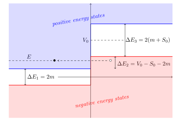
Figure 1: The gap between positive and negative energies for $V_{0}-S_{0}>2m$. To the left of the barriers, the energy E is located in the domain of positive energies. To the right of the steps, E is located in the range of negative energies. This leads to the Klein’s paradox.

Let us first consider the case with $V_{0}>2m+S_{0}$. In this case, we have three ranges for the energy $E$.

1. The first range is defined by $E>V_{0}+m+S_{0}$. As long as $E>V_{0}+m+S_{0}$, the parameter $\gamma_{s}>0$ and we have

   $$R=\left|\frac{j_{ref}}{j_{inc}}\right|=\left|\bar{r}\right|^{2}=\left(\frac{1-\gamma_{s}}{1+\gamma_{s}}\right)^{2}$$ (15)

   and

   $$T=\left|\frac{j_{trans}}{j_{inc}}\right|=\left|\bar{t}\right|^{2}=\frac{4\left|\gamma_{s}\right|}{\left(1+\gamma_{s}\right)^{2}}$$ (16)

   Here, we can check that $R<1$ and

   $$R+T=1$$ (17)

2. The second range is when $V_{0}-m-S_{0}<E<m+S_{0}+V_{0}$. In such a case, the wave vector $q$ to the right of the barriers is imaginary and the solution decays exponentially. In particular, when $E-V_{0}<<m$, then the solution $\exp(-\left|q\right|z)$ is localized to within a few Compton wavelengths. We have complete reflection with exponential penetration into the classically forbidden region.

3. The third range is the so-called Klein’s zone, when $V_{0}-m-S_{0}>E>m$. Here, according to (8), $q$ becomes real and we obtain an oscillating transmitted plane wave. This is the first manifestation of the Klein paradox. This surprising result is due to the fact that the solutions with $V_{0}-m-S_{0}>E>m$ are positive energy solutions in the first region and negative energy solution in the second region. Consequently, instead of complete reflection with exponential penetration into the classically forbidden region, we have a transition into negative energy states with $E<V_{0}-m-S_{0}$.

   If the potential is strong enough, $V_{0}>2m+S_{0}$, and $E<V_{0}-S_{0}-m$ the parameter $\gamma_{s}$ becomes negative, $\bar{\gamma}<0$, and the reflected current would be then greater than the incident current. Consequently, the flux going out to the left exceeds the incoming flux and we have

   $$R-T=1.$$ (18)

   This is an other manifestation of the Klein’s paradox [23].

   Following Feynman’s interpretation, the antiparticles are moving backward in time. Then, the wave function $\psi\approx\exp\left(iqz\right)=\exp\left[-i\left(-q\right)z\right]$  describes an antiparticle that moves to the left region [24]. This represents a total reflection of the $"in"$ (incoming) particle of the potential barrier accompanied by particle-antiparticle creation. It is said that pairs are created in the vicinity of the barrier.

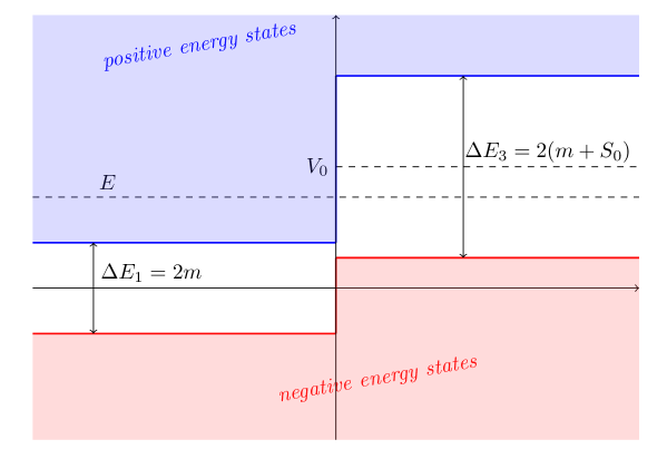
Figure 2: The gap between positive and negative energies for $V_{0}-S_{0}<2m$. To the left of the barriers, the energy E is located in the domain of positive energies. To the right of the steps, E is located in the forbidden region. The solution is then exponentially decaying.

Let us note that in the case when $2m+S_{0}>V_{0}>2m$, there is no overlap between positive energy states in the first region and negative energy states in the second region. In such a case, we have either a complete reflection with exponential penetration in the forbidden region or a transition from a positive energy state in the first region to a positive energy state in the second region. Therefore, even if $V_{0}>2m$, Klein’s paradox can not take place as long as $V_{0}<2m+S_{0}$.

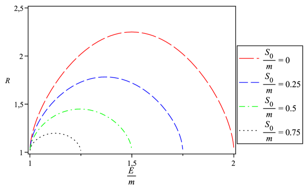
Figure 3: The variation of $R$ versus $\frac{E}{m}$. $V_{0}$ is taken $V_{0}=3m$.

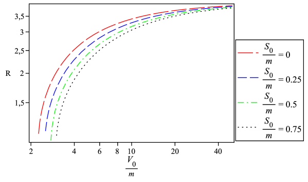
Figure 4: Plotting $R$ as function of the variable $\frac{V_{0}}{m}$ for $E=1.25m$.

Figure 5: Plotting $R$ as function of the variable $\frac{S_{0}}{m}$. $V_{0}$ and $E$ are chosen so that $\frac{V_{0}}{m}-\frac{E}{m}=2.5$.

Plotting $R$ as a function of the variables $\frac{E}{m}$, $\frac{V_{0}}{m}$ and $\frac{S_{0}}{m}$, we show that the considered scalar barrier minimizes the reflection coefficient in the Klein range. The presence of a scalar barrier shortens the Klein range. When $S_{0}$ exceeds $V_{0}-2m$, the Klein’s paradox disappears.

In the next section, we consider the Klein’s paradox and related particle creation by a vector and scalar barriers in the framework of quantum field theory.

3 Quantum fields interpretation

Obviously, the treatment of the present problem in the context of relativistic quantum mechanics has led to paradoxical results. This is because the sound approach to study quantum processes in the presence of a potential barrier is rather the quantum field theory in external fields. Following this approach, we have two different definitions of particles; The first one is based on the in-basis and the other on the out-basis. These two definitions are in general different and the difference is a consequence of the vacuum instability in the presence of the potential barriers. However, in literature we find two different definitions of the ”in” and ”out” states; The first one is suggested by Hansen and Ravndall [26] and accepted by Greiner and co-workers [27] while the second is proposed by Nikishov [28] and has been much used [9, 12, 25, 29, 30, 31, 32, 33]. Recently, a well-built quantum field theory in the presence of critical potential steps is elaborated in [25]. In that paper the authors showed that the correct definition of ”in” and ”out” states is that of Nikishov. In this section, we follow the method of [25].

3.1 The choice of ”in” and ”out” states

Let us first write the solution to the Dirac eqaution in the form

$$\psi\left(t,z\right)=e^{-iEt}\varphi\left(z\right),$$ (19)

where $\varphi\left(z\right)$ is a solution of the stationary equation (1). Besides the solution obtained in the previous section we can construct other solutions that can be interpreted as the $"in"$ and $"out"$ states of the particle and the antiparticle. We consider only the important case of the Klein zone where $m<E<V_{0}-m-S_{0}$. In this case, the ”in” and ”out” particles are situated on the left of the step and the ”in” and ”out” antiparticles are situated on the right of the step. Then the ”in” particles that are moving to the step from the left are subjected to total reflection and the ”in” antiparticles that are moving to the step from the right are subjected to total reflection. Therefore, acording to [28] and [25] the ”out” states can be written as follows

$$\varphi_{out}^{-}\left(z\right)=N_{out}\left\{\begin{array}[]{lcc}u\left(p\right)~{}\exp(ipz),&&z<0\\ \zeta_{1}v\left(q\right)\exp(iqz)+\zeta_{2}v\left(-q\right)\exp(-iqz),&&z>0\end{array}\right.$$ (20)

and

$$\varphi_{out}^{+}\left(z\right)=N_{out}^{\ast}\left\{\begin{array}[]{lll}v\left(q\right)\exp(iqz),&&z>0\\ \zeta_{1}^{+}u\left(p\right)\exp(ipz)+\zeta_{2}^{+}u\left(-p\right)\exp(-ipz),&&z<0\end{array}\right.$$ (21)

where

$$\zeta_{1} = -\zeta_{1}^{+}=-\frac{\left(1+\gamma_{s}\right)}{2\sqrt{\left|\gamma_{s}\right|}}$$

$$\zeta_{2} = \zeta_{2}^{+}=\frac{1-\gamma_{s}}{2\sqrt{\left|\gamma_{s}\right|}}$$

and the the spinors $u\left(\pm p\right)$ and $v\left(\pm q\right)$ are given by

$$u\left(\pm p\right)=\sqrt{\frac{E+m}{2p}}\begin{pmatrix}1\\ \frac{\pm p}{E+m}\end{pmatrix}$$ (22)

and

$$v\left(\pm q\right)=\sqrt{\frac{\left(E-V_{0}\right)+\left(m+S_{0}\right)}{2\left|q\right|}}\begin{pmatrix}1\\ \frac{\pm q}{\left(E-V_{0}\right)+\left(m+S_{0}\right)}\end{pmatrix}.$$ (23)

For the ”in” states, we have

$$\varphi_{in}^{-}\left(z\right)=N_{in}\left\{\begin{array}[]{lcc}u\left(-p\right)\exp(-ipz),&&z<0\\ \zeta_{2}v\left(q\right)\exp(iqz)+\zeta_{1}v\left(-q\right)\exp(-iqz),&&z>0\end{array}\right.$$ (24)

and

$$\varphi_{in}^{+}\left(z\right)=N_{in}^{\ast}\left\{\begin{array}[]{lcc}v\left(-q\right)\exp(-iqz),&&z>0\\ \zeta_{2}^{+}u\left(p\right)\exp(ipz)+\zeta_{1}^{+}u\left(-p\right)\exp(-ipz),&&z<0\end{array}\right..$$ (25)

The constants $N_{in}$, and $N_{out}$ are determined according to standard orthogonality conditions, see Eq. (3.36) in [25],

$$\left(\psi_{in,k}^{\epsilon},\psi_{in,k^{\prime}}^{\epsilon^{\prime}}\right)_{z} = \epsilon~{}\eta_{L}\delta_{\epsilon,\epsilon^{\prime}}\delta_{k,k^{\prime}}$$ (26)

$$\left(\psi_{out,k}^{\epsilon},\psi_{out,k^{\prime}}^{\epsilon^{\prime}}\right)_{z} = \epsilon~{}\eta_{R}\delta_{\epsilon,\epsilon^{\prime}}\delta_{k,k^{\prime}}$$ (27)

where $k$ denotes the conserved quantum numbers (the energy in our case) and the scalar product of the two states is defined by, see Eq. (3.33) in [25],

$$\left(\psi^{+},\psi^{-}\right)_{z}=\int\overline{\psi^{+}}\boldsymbol{\beta\alpha}\psi^{-}dt.$$ (28)

In (26) and (27) $\eta_{L}$ and $\eta_{R}$ are defined by $\eta_{L,R}=\mathop{\mathrm{s}ign}\left(E-V_{L,R}\right)$ with

$$V_{L}=\lim_{z\rightarrow-\infty}V\left(z\right)=0\text{ \ and \ \ \ }V_{R}=\lim_{z\rightarrow+\infty}V\left(z\right)=V_{0}$$

Tanking into account that

$$\left|\zeta_{2}\right|^{2}-\left|\zeta_{1}\right|^{2}=1$$ (29)

and the spinors $u\left(p\right)$ and $v\left(q\right)$ verify the following relations

$$\overline{u\left(\epsilon p\right)}~{}\boldsymbol{\beta\alpha~{}}u\left(\epsilon^{\prime}p\right) = \epsilon~{}\delta_{\epsilon,\epsilon^{\prime}}$$ (30)

$$\overline{v\left(\epsilon q\right)}~{}\boldsymbol{\beta\alpha~{}}v\left(\epsilon q\right) = \epsilon~{}\delta_{\epsilon,\epsilon^{\prime}}$$ (31)

we find that the orthonormalization conditions (26) and (27) are fulfilled for $\left|N_{in}\right|=\left|N_{out}\right|=1$.

Let us note that this definition of the ”in” and ”out” states in the Klein zone which coincides with the one proposed by Nikishov is unrelated to considerations of the previous section.

3.2 Particle creation in the Klein’s range

Now, according to the standard $S$-matrix formalism of quantum field theory, the matter field operator admits the following two decompositions

$$\mathbf{\psi} =\underset{k}{\sum}\left(a_{in,k}~{}\psi_{in,k}^{+}+b_{in,k}^{+}~{}\psi_{in,k}^{-}\right)$$ (32)

$$=\underset{k}{\sum}\left(a_{out,k}~{}\psi_{out,k}^{+}+b_{out,k}^{+}~{}\psi_{out,k}^{-}\right)$$ (33)

where the operator $a_{in}$ ($a_{out}$) annihilates a particle in the $"in"$ ($"out"$) state and the operator $b_{in}^{+}$ ($b_{out}^{+}$) creates an antiparticle in the $"in"$ ($"out"$) state. These operators verify the following anticommutation relations

$$\left[a_{in,k},a_{in,k^{\prime}}^{+}\right]_{+} =\left[a_{out,k},a_{out,k^{\prime}}^{+}\right]_{+}=\delta_{k,k^{\prime}}$$ (34)

$$\left[b_{in,k},b_{in,k^{\prime}}^{+}\right]_{+} =\left[b_{out,k},b_{out,k^{\prime}}^{+}\right]_{+}=\delta_{k,k^{\prime}}$$ (35)

and all mixed anticommutators vanish

$$\left[a,b\right]_{+}=\left[a,b^{+}\right]_{+}=0.$$ (36)

With these two definitions of particles, the observed created particles are out-particles in the in-vacuum.

Since the set $\left\{\psi_{out}^{+}\left(z\right),\psi_{out}^{-}\left(z\right)\right\}$ forms a basis for the solution space of the equation (1), we can write the elements of the second set $\left\{\psi_{in}^{+}\left(z\right),\psi_{in}^{-}\left(z\right)\right\}$ as linear combinations of the functions $\psi_{out}^{+}\left(z\right)$ and $\psi_{out}^{-}\left(z\right)$. Indeed, taking into account that the spinors $u\left(\pm p\right)$ and $v\left(\pm q\right)$ verify the following relations

$$v\left(q\right) = \zeta_{1}^{+}u\left(p\right)+\zeta_{2}^{+}u\left(-p\right)$$

$$v\left(-q\right) = \zeta_{2}^{+}u\left(p\right)+\zeta_{1}^{+}u\left(-p\right)$$

$$u\left(p\right) = \zeta_{2}^{+}v\left(-q\right)-\zeta_{1}^{+}v\left(q\right)$$

$$u\left(-p\right) = \zeta_{2}v\left(q\right)+\zeta_{1}v\left(-q\right)$$

we easily establish the developments

$$\varphi_{in}^{+}\left(z\right) = \alpha^{\ast}\varphi_{out}^{+}\left(z\right)+\beta^{\ast}\varphi_{out}^{-}\left(z\right)$$ (37)

$$\varphi_{in}^{-}\left(z\right) = \alpha\varphi_{out}^{-}\left(z\right)+\beta\varphi_{out}^{+}\left(z\right),$$ (38)

where the Bogoliubov coefficients $\alpha$ and $\beta$ are given by

$$\alpha^{\ast} = -\frac{\zeta_{1}}{\zeta_{2}}=-\frac{1+\gamma_{s}}{1-\gamma_{s}}$$ (39)

$$\beta^{\ast} = \frac{1}{\zeta_{2}}=\frac{2\sqrt{\left|\gamma_{s}\right|}}{1-\gamma_{s}}$$ (40)

with the condition

$$\left|\alpha\right|^{2}+\left|\beta\right|^{2}=1.$$ (41)

This is the Bogoliubov transformation connecting the ”in” with the ”out” states which can be written in the following equivalent form

$$\varphi_{out}^{+}\left(z\right) = \alpha\varphi_{in}^{+}\left(z\right)+\beta\varphi_{in}^{-}\left(z\right)$$ (42)

$$\psi_{out}^{-}\left(z\right) = \alpha^{\ast}\psi_{in}^{-}\left(z\right)+\beta^{\ast}\varphi_{in}^{+}\left(z\right).$$ (43)

This relation between ”in” and ”out” states can be converted to be a relation between ”in” and ”out” operators by the use of (32) and (33). We get

$$a_{in} = \alpha a_{out}+\beta^{\ast}b_{out}^{+}$$ (44)

$$b_{in}^{+} = \beta a_{out}+\alpha^{\ast}b_{out}^{+}.$$ (45)

We can also write the ”out” operators in terms of the ”in” operators

$$a_{out} = \alpha a_{in}+\beta^{\ast}b_{in}^{+}$$ (46)

$$b_{out}^{+} = \beta a_{in}+\alpha^{\ast}b_{in}^{+}.$$ (47)

Here, we notice that that the obtained Bogoliubov coefficients completely determine the quantum processes in the presence of a scalar barrier in addition to the usual vector barrier. This procedure allows us to calculate all physical quantities in a simple way. For instance, to deal with the particle creation process, we consider the amplitude

$$\mathcal{A}=\left\langle 0_{out}\left|a_{out}b_{out}\right|0_{in}\right\rangle$$ (48)

and by taking into account that

$$b_{out}=\frac{1}{\alpha^{\ast}}b_{in}+\frac{\beta^{\ast}}{\alpha^{\ast}}a_{out}^{+}$$ (49)

we find

$$\mathcal{A}=-\frac{\beta^{\ast}}{\alpha^{\ast}}e^{iw},$$ (50)

where $e^{iw}$ is the vacuum to vacuum amplitude

$$e^{iw}=\left\langle 0_{out}\right|\left.0_{in}\right\rangle.$$ (51)

The absolute probability to create particles in the vicinity of the barrier is then

$$P_{Cr}=\left|\mathcal{A}\right|^{2}=\left|\frac{\beta^{\ast}}{\alpha^{\ast}}\right|^{2}C_{0}=P_{rel}~{}C_{0}$$ (52)

where $C_{0}$ is the vacuum to vacuum probability

$$C_{0}=\left|\left\langle 0_{out}\right|\left.0_{in}\right\rangle\right|^{2}$$ (53)

and $P_{rel}$ is the relative probability to create a pair

$$P_{rel}=\left|\frac{\beta^{\ast}}{\alpha^{\ast}}\right|^{2}=\frac{4\left|\gamma_{s}\right|}{\left(1+\gamma_{s}\right)^{2}}$$ (54)

Taking into account the Pauli exclusion principle, we have

$$C_{0}+\left|\frac{\beta^{\ast}}{\alpha^{\ast}}\right|^{2}C_{0}=1,$$ (55)

which gives, directly, the vacuum persistence (vacuum to vacuum probability)

$$C_{0}=\frac{1}{1+\left|\frac{\beta^{\ast}}{\alpha^{\ast}}\right|^{2}}=\left|\alpha\right|^{2}=\left(\frac{1+\gamma_{s}}{1-\gamma_{s}}\right)^{2}.$$ (56)

We, therefore, have

$$P_{Cr}=\left|\frac{\beta^{\ast}}{\alpha^{\ast}}\right|^{2}~{}\left|\alpha\right|^{2}=\left|\beta\right|^{2}=\frac{4\left|\gamma_{s}\right|}{\left(1-\gamma_{s}\right)^{2}}=\frac{T}{R}.$$ (57)

Another important result of the Pauli principle is that only one pair could be created in well-defined state. The mean number of created particles in the state $E$ is then

$$\overline{n}=P_{rel}~{}C_{0}=\left|\beta\right|^{2}=\frac{4\left|\gamma_{s}\right|}{\left(1-\gamma_{s}\right)^{2}},$$ (58)

which is the same as the mean number of ”out” particles in the ”in” vacuum $\overline{n}=\left\langle 0_{in}\left|a_{out}^{+}a_{out}\right|0_{in}\right\rangle=\left|\beta\right|^{2}$.

In Figure (6) we plot the absolute probability $P_{Cr}$ as a function of the variable $\frac{S_{0}}{m}$ for several values of $\frac{E}{m}$ and $\frac{V_{0}}{m}$ with $V_{0}=E+2.5m$. The result is as expected, the scalar barrier, as considered in this paper, minimizes the absolute particle creation probability.

Figure 6: Plotting the probability $P_{Cr}$ as a function of the variable $\frac{S_{0}}{m}$ for several values of $\frac{E}{m}$.

In Figure (7) we plot the absolute probability $P_{Cr}$ as a function of the variable $\frac{V_{0}}{m}$ for several values of $\frac{S_{0}}{m}$ and $\frac{V_{0}}{m}$ with $V_{0}=E+2.5m$. In addition to reducing the particle creation, plots in Figure (7) show also that as $V_{0}$ increase as the effect of the scalar barrier becomes inessential.

Figure 7: Plotting the probability $P_{Cr}$ as a function of the variable $\frac{V_{0}}{m}$ for several values of $\frac{S_{0}}{m}$.

4 Conclusion

We have studied, in this paper, the Klein’s paradox in the presence of scalar and vector potential barriers. At the first stage, we have found the exact solutions of the corresponding Dirac equation. Then, we have extracted form these solutions the transmission and reflection coefficients. It is shown that the presence of a scalar barrier in addition to the vector one minimizes the reflection coefficient in the Klein range. The presence of a scalar barrier shortens the Klein range. When $S_{0}$ exceeds $V_{0}-2m$, the Klein’s paradox disappears.

In order to get the good interpretation of the pair creation we have considered a field theoretical treatment following the rigorous theory elaborated in [25]. At the first stage, we have defined the ”in” and ”out” states. Then, we were able to extract the Bogoliubov coefficients and to calculate the pair production probability and the mean density of created particles. We have shown that the scalar potential decreases the relative probability to create a pair of particles. This result can be explained by the fact that the gap between positive and negative energies in the region $(z>0)$ in the presence of the vector potential is $2m$ while this gap becomes  $2m+2S_{0}$ in the presence of the scalar potential. This means that, in the presence of the scalar potential, the forbidden band to the right of the barrier is larger than the usual one and therefore, the scalar potential cut down the Klein range and minimizes the creation of particles. The particle creation decreases as the scalar potential increases and ceases definitely when the scalar potential reaches the value $V_{0}-2m$. In other words, in the presence of scalar and vector barriers, only particles of mass $m$, with $2m<V_{0}-S_{0}$, can be created.

Theoretically, this result could have a significant impact in nuclear physics; In the case of spin and pseudospin symmetries where the magnitudes of the scalar and vector potentials are equal [34, 35, 36], the Klein range would be suppressed by the scalar potential and the creation of particles by the tunneling mechanism would then be impossible.

References

- [1] J. D. Bjorken and S. D. Drell, Relativistic Quantum Fields (Mc Graw Hill, New York, 1965)
- [2] W. Greiner, Relativistic Quantum Mechanics (Springer, Berlin, 2000)
- [3] V. G. Bagrov and D. M. Gitman, Exact Solutions of Relativistic Wave Equations,(Kluwer, Dordrecht 1990)
- [4] O. Klein, Z. Phys. 53, 157 (1929).
- [5] A. Calogeracos, N. Dombey, Contemp. Phys. 40, 313 (1999).
- [6] C. Xu, and Y. J. Li, arXiv: hep-ph/1504.00901
- [7] F. Sauter, Z. Phys. 73, 547 (1931)
- [8] A. I. Nikishov, Nucl. Phys. B 21, 346 (1970)
- [9] S. P. Gavrilov, D. M. Gitman, A. A. Shishmarev, Phys. Rev. D 99, 116014 (2019)
- [10] A. I. Nikishov, Problems of atomic science and technology, Special issue dedicated to the 90-birthday anniversary of A. I. Akhieser, Kharkov, Ukraine, p.103 (2001)
- [11] M. Merad, L. Chetouani, A. Bounames, Phys. Lett. A 267, 225 (2000)
- [12] S. Haouat and L. Chetouani, Eur. Phys. J. C 41, 297 (2005)
- [13] A. Bounames, L. Chetouani, Phys. Lett. A 267, 225 (2000)
- [14] L Chetouani, M. Merad, T. Boudjedaa, A. Lecheheb, Int. J. Theor. Phys. 43, 1147 (2004)
- [15] M. Merad, Int. J. Theor. Phys. 46, 2105 (2007)
- [16] T. R. Cardoso, L. B. Castro, A. S. de Castro, Can. J Phys. 87, 1185 (2009)
- [17] A. S. de Castro, Phys. Lett. A 309, 340 (2003)
- [18] S. Haouat and L. Chetouani, Hadronic Journal 29, 697 (2006)
- [19] S. Haouat and M. Benzekka, Phys. Lett. A 377, 2255 (2013)
- [20] W. M. Castilho and A. S. de Castro, Annals Phys. 346, 164 (2014)
- [21] W. M. Castilho and A. S. de Castro, Eur. Phys. J. Plus 131, 94 (2016)
- [22] W. M. Castilho and A. S. de Castro, Annals Phys. 340, 1 (2014)
- [23] F. Schwabl, Advanced Quantum Mechanics (Springer-Verlag Berlin Heidelberg , Berlin, 2008)
- [24] B. R. Holstein, Am. J. Phys. 66, 507 (1998).
- [25] S.P. Gavrilov and D.M. Gitman, Phys. Rev. D 93, 045002 (2016)
- [26] A. Hansen and F. Ravndal, Phys. Scr. 23, 1036 (1981).
- [27] W. Greiner, B. Muller and J. Rafelski, Quantum Electrodynamics of Strong Fields (Springer-Verlag, Berlin, 1985).
- [28] A. I. Nikishov, Phys. Atom. Nucl. 67, 1478 (2004).
- [29] S. P. Gavrilov and D. M. Gitman, Int. J. Mod. Phys. A 31, 1641031 (2016).
- [30] S. P. Gavrilov, D. M. Gitman, A. A. Shishmarev, Phys. Rev. D 96, 096020 (2017)
- [31] S. P. Gavrilov, D. M. Gitman, A. A. Shishmarev, Phys. Rev. D 93, 105040 (2016)
- [32] S. P. Gavrilov and D. M. Gitman, Phys. Rev. D 93, 045033 (2016)
- [33] D. M. Gitman and S. P. Gavrilov, Russian J Phys. 59, 1723 (2016)
- [34] J. N. Ginocchio, Phys. Rev. Lett. 78, 436 (1997)
- [35] J. N. Ginocchio and A. Leviatan, Phys. Lett. B 425, 1 (1998)
- [36] J. N. Ginocchio and A. Leviatan, Phys. Rev. Lett. 87, 072502 (2001)