A new method for measuring angle-resolved phases in photoemission

Abstract

Quantum mechanically, photoionization can be fully described by the complex photoionization amplitudes that describe the transition between the ground state and the continuum state. Knowledge of the value of the phase of these amplitudes has been a central interest in photoionization studies and newly developing attosecond science, since the phase can reveal important information about phenomena such as electron correlation. We present a new attosecond-precision interferometric method of angle-resolved measurement for the phase of the photoionization amplitudes, using two phase-locked Extreme Ultraviolet pulses of frequency $\omega$ and $2\omega$, from a Free-Electron Laser. Phase differences $\Delta\tilde{\eta}$ between one- and two-photon ionization channels, averaged over multiple wave packets, are extracted for neon $2p$ electrons as a function of emission angle at photoelectron energies 7.9, 10.2, and 16.6 eV. $\Delta\tilde{\eta}$ is nearly constant for emission parallel to the electric vector but increases at 10.2 eV for emission perpendicular to the electric vector. We model our observations with both perturbation and ab initio theory, and find excellent agreement. In the existing method for attosecond measurement, Reconstruction of Attosecond Beating By Interference of Two-photon Transitions (RABBITT), a phase difference between two-photon pathways involving absorption and emission of an infrared photon is extracted. Our method can be used for extraction of a phase difference between single-photon and two-photon pathways and provides a new tool for attosecond science, which is complementary to RABBITT.

I Introduction

The age of attosecond physics was ushered in by the invention of methods for probing phenomena on a time scale less than femtoseconds Krausz and Ivanov (2009). A phenomenon occurring on this time scale is photoemission delay. When the photon energy is far from resonance, the photoemission delay for single photon ionization can be associated with the Wigner delay experienced by an electron scattering off the ionic potential Wigner (1955). Quantum mechanically, the photoionization process is fully described by the complex photoionization amplitudes describing transitions between the ground state and the continuum state. The photoemission delay can be expressed as the energy derivative of the phase of the photoionization amplitude, and therefore measuring the photoemission delay and the energy-dependent phase of the photoionization amplitude are practically equivalent. Their measurement is one of the central interests in attosecond science Pabst and Dahlström (2016); Klünder et al. (2011); Guénot et al. (2014, 2012); Palatchi et al. (2014); Kheifets (2013); Saha et al. (2014); Argenti et al. (2017); Busto et al. (2019); Vos et al. (2018); Azoury et al. (2019a); Fuchs et al. (2020), because they are a fundamental probe of the photoionization process and can reveal important information about, for example, electron-electron correlations (see, e.g. Ossiander et al. (2017)).

Currently two methods are available to measure these quantities: streaking and RABBITT (Reconstruction of Attosecond Beating By Interference of Two-photon Transitions), both of which require the use of an IR dressing field. We present a new interferometric method of angle-resolved measurement for the photoionization phase, using two phase-locked Extreme Ultraviolet (XUV) pulses of frequency $\omega$ and $2\omega$, from a Free-Electron Laser (FEL), without a dressing field.

In attosecond streaking Schultze et al. (2010), an ultrafast, short-wavelength pulse ionizes an electron, and a femtosecond infrared (IR) pulse acts as a streaking field, by changing the linear momentum of the photoelectron. In this technique, one can extract the photoemission delay difference between two photoemission lines at two different energies, arising for example from two different subshells Schultze et al. (2010) or the main line and satellites Ossiander et al. (2017). Generally, time-of-flight electron spectrometers located in the streaking direction (the direction of linear polarization) are used, so that this method does not give access to angular information. A related method is the attosecond clock technique Eckle et al. (2008a, b); Pfeiffer et al. (2012, 2011), in which streaking by the circularly polarized laser pulse is in the angular direction.

The second technique for measuring photoemission delays, RABBITT, is interferometric: it uses a train of attosecond pulses dressed by a phase-locked IR pulse Paul et al. (2001). In the RABBITT technique, the phase difference between a pair of two-photon pathways whose final energy is separated by multiples of an infrared photon energy is extracted. The extracted value is related to the phase difference of the two-photon ionization amplitudes at the pair of energies. For two energy points separated by twice the IR photon energy, the phase difference divided by twice the IR photon energy can be regarded as a finite difference approximation to the energy derivative of phase of the two-photon ionization amplitude. The pulse duration requirements are relaxed: for example, pulse trains and IR pulses of 30 fs duration may be used Guénot et al. (2012). Usually the IR pulse is the fundamental of the odd harmonics in the pulse train, although Loriot et al. (2017) reported a variant using the second harmonic. Recent work on phase retrieval includes methods based on photo-recombination Azoury et al. (2019a, b), two-color, two-photon ionization via a resonance Villeneuve et al. (2017), and a proposal to use successive harmonics of circularly polarized light Donsa et al. (2019).

The phase of the photoionization amplitude depends on photoelectron energy $\epsilon$ and it may also depend on the electron’s emission direction. There is a physical origin for the directional anisotropy of the amplitude: an electron wave packet may consist of two or more partial waves, with different angular momenta and phases. There has been significant theoretical work on the angle-dependent time delay, for example Ref. [Dahlström and Lindroth, 2014; Wätzel et al., 2015; Heuser et al., 2016; Mandal et al., 2017; Ivanov and Kheifets, 2017; Bray et al., 2018; Banerjee et al., 2019], but fewer related experimental reports Heuser et al. (2016); Cirelli et al. (2018); Vos et al. (2018), all using the RABBITT technique. The Wigner delay is theoretically isotropic for single-photon ionization of He, but Heuser et al. (2016) observed an angular dependence in photoemission delay, attributed to the XUV+IR two-photon ionization process, inherent in RABBITT interferometry.

In the present work, we demonstrate interferometric measurements of the relative phase of single-photon and two-photon ionization amplitudes. The interference is created between a two-photon ionization process driven by a fundamental wavelength, and a single-photon ionization process driven by its phase-locked, weaker, second harmonic, in a setup like that demonstrated at visible wavelengths Shapiro and Brumer (2003). Using short-wavelength, phase-locked XUV light, we measure angular distributions of photoelectrons emitted from neon, and determine the phase difference for one- and two-photon ionization wavepackets. The extremely short (attoseconds) pulses required for streaking or attosecond pulse trains for RABBITT are not needed, and instead access to photoemission phase with attosecond precision is provided by optical phase control with precision of a few attoseconds, which is available from the Free-Electron Laser FERMI Prince et al. (2016).

The rest of the manuscript is structured as follows: in Section II we introduce the necessary notation and the basic processes that may be active in the experiment; in Section III and IV we describe respectively the experimental and theoretical methods used. In Section V we present and compare experimental and theoretical results. We discuss in Section VI the relationship between our data, namely the angular distribution of photoelectrons created by collinearly polarized biharmonics, and the time-delay studies described in the introductory section. Section VII presents our summary and outlook, and the Appendix gives details of the derivation of some equations.

II Notation and basic processes

We use Hartree atomic units unless otherwise stated, and spherical coordinates $\textbf{r}=\{r,\theta,\varphi\}$ relative to the direction of polarization of the bichromatic field (linear horizontal in the experiment). We assume the electric dipole approximation, and the experiment is cylindrically symmetric about the electric vector, so that there is no dependence on the azimuthal angle $\varphi$. The bichromatic electric field is described by:

$$E\left(t\right)=\sqrt{I_{\omega}\left(t\right)}\cos\omega t+\sqrt{I_{2\omega}\left(t\right)}\cos\left(2\omega t-\phi\right)\,,$$ (1)

where $\omega$ and $2\omega$ are angular frequencies, $I_{\omega}(t)$ and $I_{2\omega}(t)$ are the pulse envelopes, $\phi$ denotes the $\omega$-$2\omega$ relative phase.

We can consider the experimental sample as an ensemble of identical atoms of infinitesimal size, so we can reduce the theoretical treatment to that of a single atom centered at the coordinates’ origin. The general form (omitting as implicit the dependence on $\theta,\varphi$) of an electron wave packet sufficiently far away from the origin is:

$$\int_{0}^{\infty}c(\epsilon)\,e^{-i\epsilon t}e^{i\left[\sqrt{2\epsilon}\,r+f(r,\epsilon)+\eta(\epsilon)\right]}d\epsilon\,,$$ (2)

where $\epsilon$ is the photoelectron kinetic energy, $c(\epsilon)$ the real-valued amplitude, $\eta(\epsilon)$ the phase, and the term $f(r,\epsilon)=\frac{Z}{\sqrt{2\epsilon}}\ln\sqrt{8\epsilon}\,r$ accounts for the Coulomb field of the residual ion with charge $Z$. In our case $Z=+1$.

In the $\omega$-$2\omega$ process, i.e., one driven by the field in Eq. (1), the wave packet can be expressed as

$$\int_{0}^{\infty}c(\epsilon)\,e^{-i\epsilon t}e^{i\left[\sqrt{2\epsilon}\,r+f(r,\epsilon)\right]}\{c_{\omega}(\epsilon)e^{i\eta_{\omega}(\epsilon)}+c_{2\omega}(\epsilon)e^{i[\eta_{2\omega}(\epsilon)+\phi]}\}d\epsilon\,.$$ (3)

The photoelectron yield as a function of optical phase $\phi$ (we omit the spatial coordinates on the right-hand side) is given by

$$I(\theta,\varphi;\phi)\doteq I(\theta;\phi) = \int_{0}^{\infty}c_{\omega}(\epsilon)^{2}+c_{2\omega}(\epsilon)^{2}+2c_{\omega}(\epsilon)c_{2\omega}(\epsilon)\cos\left[\phi-\Delta\eta\left(\epsilon\right)\right]\,d\epsilon$$ (4)

$$\equiv A_{0}+A\cos\left[\phi-\Delta\eta\left(\bar{\epsilon}\right)\right],$$

where $\bar{\epsilon}$ is the average kinetic energy of the wave packet, and $\Delta\eta\left(\epsilon\right)\equiv\eta_{\omega}(\epsilon)-\eta_{2\omega}(\epsilon)$ is the phase of the two-photon ionization relative to the single-photon ionization.

This treatment may be generalized to the case of multiple wave packets, that is to say, with more than one magnetic quantum number $m$ of the residual ion. Wave packets with each value of $m$ interfere separately, and then incoherently add. In particular, expressing the photoionization yield as in Eq. (4)

$$I(\theta;\phi)=A_{0}+A\cos\left(\phi-\Delta\tilde{\eta}\right)=\sum_{m}[A_{0,m}+A_{m}\cos(\phi-\Delta\eta_{m})],$$ (5)

where summation is over the wave packets, leading to

$$A_{0}=\sum_{m}A_{0,m},\qquad Ae^{i\Delta\tilde{\eta}}=\sum_{m}A_{m}e^{i\Delta\eta_{m}}.$$ (6)

The second equation defines an average phase difference $\Delta\tilde{\eta}$ of $\{\Delta\eta_{m}\}$, weighted in terms of the corresponding phase factors. Eqs. (4) and (5) indicate that the yield of photoelectrons emitted by a bichromatic pulse in a particular direction oscillates sinusoidally as a function of the optical phase $\phi$.

III Experimental Methods and Setup

The experimental methods have been described elsewhere Prince et al. (2016) and here we summarise the main aspects, and the parameters used. The experiment was carried out at the Low Density Matter Beamline Lyamayev et al. (2013); Svetina et al. (2015) of the FERMI Free-Electron Laser Allaria et al. (2015), using the Velocity Map Imaging (VMI) spectrometer installed there. The VMI measures the projection of the Photoelectron Angular Distribution (PAD) onto the planar detector (horizontal); the PAD is obtained as an inverse Abel transform of this projection, using the BASEX method Dribinski et al. (2002). The images were divided into two halves along the line of the electric vector, labelled “left” and “right”, and analysed separately. The PADs from the two halves agreed generally, but the detector for the right half showed a small non-uniformity in detection efficiency. Therefore the PADs were analysed using the left half of the detector, denoted as 0 - 180^∘ below.

The sample consisted of a mixture of helium and neon, and the helium PAD was used to calibrate the phase difference between the $\omega$ and $2\omega$ fields. The atomic beam was produced by a supersonic expansion and defined by a conical skimmer and vertical slits. The length of the interaction volume along the light propagation direction was approximately 1 mm. In other experiments Guénot et al. (2014); Palatchi et al. (2014), use of two gases allowed referencing of the photoemission delay of one electron to that of another. In the present case, we used the admixture of helium to provide a phase reference. When the Free-Electron Laser wavelength is changed, the mechanical settings of the magnetic structures (undulators) creating the light are changed. This may introduce an unknown phase error between fundamental and second harmonic light. We have recently shown that the PAD of helium $1s$ electrons can be used to determine the absolute optical phase difference between the $\omega$ and $2\omega$ fields, with input of only few theoretical parameters Di Fraia et al. (2019).

The light beam consisted of two temporally overlapping harmonics with controlled relative phase $\phi$, Eq. (1), and irradiated the sample, as shown schematically in Fig. 1. The intense fundamental radiation caused two-photon ionization, while the weak second harmonic gave rise to single-photon ionization. The energies of the photoelectrons created coherently in the two channels are identical, and electrons with the same linear momentum interfere Villeneuve et al. (2017). The PAD $I\left(\theta;\phi\right)$ was measured as a function of the phase $\phi$; from the component oscillating with $\phi$, the scattering phases were extracted, as shown in Section V. The wavelength was then changed and the measurement repeated.

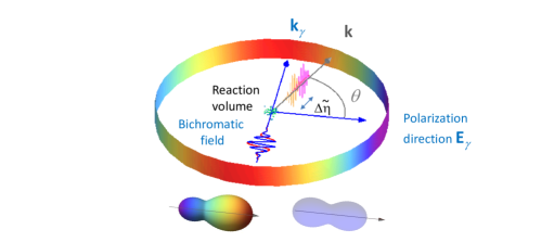
Figure 1: Scheme of the experiment: bichromatic, linearly polarized light (red and blue waves), with momentum ${\bf k}_{\gamma}$ and electric vector ${\bf E}_{\gamma}$, ionizes neon in the reaction volume. The electron wave packets (yellow and magenta waves) are emitted with electron momentum ${\bf k}$. The $m$-averaged phase difference $\Delta\tilde{\eta}$ between wavepackets created by one- and two-photon ionization depends on emission angle. The photoelectron angular distribution depends on the relative (optical) $\omega$-$2\omega$ phase $\phi$. Lower figures: polar plots of photoelectron intensity at $E_{\rm k}=16.6$ eV for coherent harmonics (asymmetric, coloured plot) and incoherent harmonics (symmetric, grey plot).

The relative phase of the two wavelengths was controlled by means of the electron delay line or phase shifter Diviacco et al. (2011); Prince et al. (2016) used previously. It has been calculated that the two pulses have good temporal overlap with slightly different durations and only a small mean variation of the relative phase of two wavelengths within the Full Width at Half Maximum of the pulses, for example 0.07 rad for a fundamental photon energy of 18.5 eV Prince et al. (2016).

The intensities of the two wavelengths for the experiments were set as follows. With the last undulator open (that is, inactive), the first five undulators were set to the chosen wavelength of the first harmonic. A small amount of spurious second harmonic radiation (intensity of the order 1% of the fundamental) is produced by the undulators Giannessi et al. (2018), and to absorb this, the gas filter available at FERMI was filled with helium. Helium is transparent at all of the fundamental wavelengths used in this study. The two-photon photoelectron signal from the neon and helium gas sample was observed with the VMI spectrometer. The last undulator was then closed to produce the second harmonic and the photoelectron spectrum of the combined beams was observed. The single-photon ionization by the second harmonic is at least an order of magnitude stronger than the two-photon ionization by the fundamental. The helium gas pressure in the gas filter was then adjusted to achieve a ratio of the ionization rates due to two-photon and single-photon ionization of 1:2 for kinetic energies of 7.0 and 10.2 eV. For the kinetic energy of 15.9 eV, the ratio was set to 1:4. The bichromatic beam was focused by adjusting the curvature of the Kirkpatrick-Baez active optics Zangrando et al. (2015), and verified experimentally by measuring the focal spot size of the second harmonic with a Hartmann wavefront sensor. This instrument was not able to measure the spot size of the beams at the fundamental wavelengths, so it was calculated Raimondi et al. (2013). The measured spot was elliptical with a size $(4.5\pm 1)\times(6.5\pm 1)$ $\mu$m² (FWHM), and the estimated pulse duration was 100 fs.

Table 1 summarizes the experimental parameters: fundamental photon energy ($\hbar\omega$), kinetic energy ($E_{\mathrm{k}}=2\hbar\omega-21.6$ eV) of the Ne photoelectrons emitted via single-photon (2$\omega)$ or two-photon ($\omega+\omega$) ionization, average pulse energy of the first harmonic at the source and at the sample, beamline transmission, and average irradiance at the sample calculated from the above spot sizes and pulse durations.

Table 1: Experimental parameters. $E_{\mathrm{k}}$ is the kinetic energy of the Ne $2p$ photoelectrons. The pulse energies at the sample were calculated by multiplying the values at the source by the transmission of the beamline Svetina et al. (2015), which takes account of reflection and geometric losses. Pulse energies and irradiance are those of the fundamental.

$\hbar\omega$, eV	$E_{\mathrm{k}}$, eV	Pulse energy, $\mu$J	Beamline	Pulse energy, $\mu$J	Average irradiance
		(at source)	transmission	(at sample)	W/cm2
14.3	7.0	45	0.10	4.5	$2.3\times 10^{14}$
15.9	10.2	95	0.13	12.4	$6.2\times 10^{14}$
19.1	16.6	84	0.23	19.3	$9.5\times 10^{14}$

The estimate of the pulse energy at $\hbar\omega$=14.3 eV was indirect, since the FERMI intensity monitors do not function at this energy, because they are based on ionization of nitrogen gas, and the photon energy is below the threshold for ionization. The method employed was to first use the in-line spectrometer to measure spectra at 15.9 eV energy and simultaneously the pulse energies from the gas cell monitors, which gave a calibration of the spectrometer intensity versus pulse energy at this wavelength. Then spectrometer spectra were measured at 14.3 eV, and corrected for grating efficiency and detector sensitivity, to yield pulse energies.

IV Theory

We now consider the physics of the experiment from two theoretical points of view: real-time ab initio simulations, which are very accurate, but computationally expensive; and perturbation theory, which allows us to explore the physics analytically and gain insights with relatively low computational costs.

IV.1 Real-time ab initio simulations

We numerically computed the photoionization of Ne irradiated by two-color XUV pulses, using the time-dependent complete-active-space self-consistent field (TD-CASSCF) method Sato and Ishikawa (2013); Sato et al. (2016), and the parameters in Table 2. The pulse length was chosen to be 10 fs for reasons of computational economy. It has been shown that the pulse length does not affect the result, provided the photoionization is non-resonant, i.e. no resonances occur within the photon bandwidth Ishikawa and Ueda (2012, 2013). As a further check, we also calculated the phase shift difference at 14.3 eV photon energy for pulse durations of 5, 10 and 20 fs, and found identical results. Thus we can safely scale the results to the present longer experimental pulses.

Neither the absolute intensity nor the ratio of intensities of the harmonics influences the calculated phase, as we show below. The dynamics of the laser-driven multielectron system is described by the time-dependent Schrödinger equation (TDSE):

$$i\frac{\partial\Psi(t)}{\partial t}=\hat{H}(t)\Psi(t),$$ (7)

where the time-dependent Hamiltonian is

$$\hat{H}(t)=\hat{H}_{1}(t)+\hat{H}_{2},$$ (8)

with the one-electron part

$$\hat{H}_{1}(t)=\sum_{i=1}^{Z}\hat{h}({\bf r}_{i},t)$$ (9)

and the two-electron part

$$\hat{H}_{2}=\sum_{i=1}^{Z}\sum_{j<i}\frac{1}{|{\bf r}_{i}-{\bf r}_{j}|}.$$ (10)

We employ the velocity gauge for the laser-electron interaction in the one-body Hamiltonian:

$$\hat{h}({\bf r},t)=\frac{{\bf k}^{2}}{2}+{\bf A}(t)\cdot{\bf k}-\frac{Z}{|{\bf r}|},$$ (11)

where ${\bf A}(t)=-\int{\bf E}(t)dt$ is the vector potential, and ${\bf E}(t)$ is the laser electric field, see Eq. (1), and $Z$ (=10 for Ne) the atomic number.

Table 2: Parameters used for theoretical calculations. $I_{\omega}$ and $I_{2\omega}$ are the peak intensities of the fundamental and second harmonic respectively.

$\hbar\omega$, eV	$I_{\omega}$, W/cm2	$I_{2\omega}$, W/cm2
14.3	$1\times 10^{13}$	$2.32\times 10^{8}$
15.9	$1\times 10^{13}$	$1.18\times 10^{8}$
19.1	$1\times 10^{13}$	$2.82\times 10^{8}$

In the TD-CASSCF method, the total electronic wave function is given in the configuration interaction (CI) expansion:

$$\Psi({x}_{1},{x}_{2},\cdots,{x}_{N},t)=\sum_{I}C_{I}(t)\Phi_{I}({x}_{1},{x}_{2},\cdots,{x}_{N},t).$$ (12)

where $x_{n}=\{{\bf r}_{n},\sigma_{n}\}$ is the joint designation for spatial and spin coordinates of the $n$-th electron. The electronic configuration $\Phi_{I}({x}_{1},{x}_{2},\cdots,{x}_{N},t)$ is a Slater determinant composed of spin orbital functions $\{\psi_{p}({\bf r},t)\times s(\sigma)\}$, where $\{\psi_{p}({\bf r},t)\}$ and $\{s(\sigma)\}$ denote spatial orbitals and spin functions, respectively. Both the CI coefficients $\{C_{I}\}$ and orbitals vary in time.

The TD-CASSCF method classifies the spatial orbitals into three groups: doubly occupied and time-independent frozen core (FC), doubly occupied and time-dependent dynamical core (DC), and fully correlated active orbitals:

$$\Psi=\hat{A}\left[\Phi_{\rm fc}\Phi_{\rm dc}\sum_{I}\Phi_{I}C_{I}\right],$$ (13)

where $\hat{A}$ denotes the antisymmetrization operator, $\Phi_{\rm fc}$ and $\Phi_{\rm dc}$ the closed-shell determinants formed with numbers $n_{\rm fc}$ FC orbitals and $n_{\rm dc}$ DC orbitals, respectively, and $\{\Phi_{I}\}$ the determinants constructed from $n_{\rm a}$ active orbitals. We consider all the possible distributions of active electrons among active orbitals. Thanks to this decomposition, we can significantly reduce the computational cost without sacrificing the accuracy in the description of correlated multielectron dynamics. The equations of motion that describe the temporal evolution of the CI coefficients $\{C_{I}\}$ and the orbital functions $\{\psi_{p}\}$ are derived by use of the time-dependent variational principle Sato and Ishikawa (2013). The numerical implementation of the TD-CASSCF method for atoms is detailed in Refs. Sato et al. (2016); Orimo et al. (2018).

IV.2 Extraction of the photoelectron angular distribution and the phase shift difference

From the obtained time-dependent wave functions, we extract the angle-resolved photoelectron energy spectrum (ARPES) by use of the time-dependent surface flux (tSURFF) method Tao and Scrinzi (2012). This method computes the ARPES from the electron flux through a surface located at a certain radius $R_{s}$, beyond which the outgoing flux is absorbed by the infinite-range exterior complex scaling Scrinzi (2010); Orimo et al. (2018).

We introduce the time-dependent momentum amplitude $a_{p}(\boldsymbol{k},t)$ of orbital $p$ for photoelectron momentum ${\bf k}$, defined by

$$a_{p}({\bf k},t)=\mbox{$\langle\chi_{\bf k}({\bf r},t)\,|\,u(R_{s})\;|\;\psi_{p}({\bf r},t)\rangle$}\equiv\int_{r>R_{s}}\chi_{{\bf k}}^{*}({\bf r},t)\psi_{p}({\bf r},t)d^{3}{\bf r},$$ (14)

where $\chi_{{\bf k}}({\bf r},t)$ denotes the Volkov wavefunction, and $u(R_{s})$ the Heaviside function which is unity for $r>R_{s}$ and vanishes otherwise. The use of the Volkov wavefunction implies that we neglect the effects of the Coulomb force from the nucleus and the other electrons on the photoelectron dynamics outside $R_{s}$, which has been confirmed to be a good approximation Orimo et al. (2019). The photoelectron momentum distribution $\rho({\bf k})$ is given by

$$\rho({\bf k})=\sum_{pq}a_{p}({\bf k},\infty)a_{q}^{*}({\bf k},\infty)\mbox{$\langle\Psi(t)\,|\,\hat{E}^{q}_{p}\;|\;\Psi(t)\rangle$},$$ (15)

with $\hat{E}^{q}_{p}\equiv\sum_{\sigma}\hat{a}_{q\sigma}^{\dagger}\hat{a}_{p\sigma}$. One obtains $a_{p}({\bf k},\infty)$ by numerically integrating:

$$-i\frac{\partial}{\partial t}a_{p}({\bf k},t)=\mbox{$\langle\chi_{{\bf k}}(t)\,|\,[\hat{h}_{s},u(R_{s})]\;|\;\psi_{p}(t)\rangle$}+\sum_{q}a_{q}({\bf k},t)\{\mbox{$\langle\psi_{q}(t)\,|\,\hat{F}\;|\;\psi_{p}(t)\rangle$}-R^{q}_{p}\},$$ (16)

where $\hat{h}_{s}=\frac{{\bf k}^{2}}{2}+{\bf A}(t)\cdot{\bf k}$, $R^{q}_{p}=i\mbox{$\langle\,\psi_{q}\,|\,\dot{\psi}_{p}\,\rangle$}-\mbox{$\langle\psi_{q}\,|\,\hat{h}\;|\;\psi_{p}\rangle$}$, and $\hat{F}$ denotes a nonlocal operator describing the contribution from the inter-electronic Coulomb interaction Sato et al. (2016); Orimo et al. (2018). The numerical implementation of tSURFF to TD-CASSCF is detailed in Ref. [Orimo et al., 2019].

We evaluate the photoelectron angular distribution $I\left(\theta;\phi\right)$ as a slice of $\rho\left({\bf k}\right)$ at the value of $\left|{\bf k}\right|$ corresponding to the photoelectron peak, and as a function of the optical phase $\phi$. Then, employing a fitting procedure very similar to that used for the experimental data, we extract the phase shift difference $\Delta\tilde{\eta}$ between single-photon and two-photon ionization at photoelectron energies 7.0 eV, 10.2 eV and 16.6 eV. The results are shown in Fig. 2.

IV.3 Perturbation theory

In the experiment, the number of optical cycles in the pulse is of the order of 400 for the fundamental and therefore we can treat the field as having constant amplitude and omit the initial phase of the field with respect to the envelope (carrier-envelope phase). Within the perturbation theory, we checked that our final results with an envelope including 100 optical cycles or more differ only within the optical linewidth from those obtained with the constant amplitude field. The bichromatic electric field is then described by Eq. (1), with time-independent $I_{\omega}$ and $I_{2\omega}$. The calculations described below were carried out for 384 optical cycles and a peak intensity of $1\times 10^{12}$ W/cm². However neither the absolute intensity nor the ratio of intensities of the harmonics influences the calculated phase, as we show below.

We make two main assumptions: the dipole approximation for the interaction of the atom with the classically described electromagnetic field, and the validity of the lowest nonvanishing order perturbation theory with respect to this interaction. These approximations are well fulfilled for neon in the FEL spectral range and intensities of interest here. We expand the amplitudes in the lowest non-vanishing order of perturbation theory in terms of matrix elements of the operator of evolution Messiah (1961). The expansion implies that in the second-order amplitude all virtual intermediate states are taken into account. Excitations of the seven lowest and most important intermediate dipole-allowed states originating from configurations ($2p^{5}$ $3s,4s,3d$) were accounted for accurately within the multiconfiguration intermediate-coupling approximation with relativistic Breit-Pauli corrections in the atomic Hamiltonian. All other virtual states (of infinite number), including those in the continuum, were accounted for by a variationally stable method Gao and Starace (1989); Staroselskaya and Grum-Grzhimailo (2015) in the Hartree-Fock-Slater approximation. More details can be found in Gryzlova et al. (2018). Further derivations within the independent particle approximation are given in the Appendix.

V Results

We extracted $\Delta\tilde{\eta}\left(\theta\right)$ from the measured PADs at three combinations of $\omega$ and $2\omega$ (corresponding to photoelectron kinetic energies, 7.0 eV, 10.2 eV and 16.6 eV), at each $5^{\circ}$ interval of polar angle. The spatial and temporal symmetry properties of the system impose constraints on the oscillatory behavior of the two emission hemispheres. Upon reflection in a plane perpendicular to the electric vector ($\theta\rightarrow\pi-\theta$), the electric field defined in Eq. (1) is inverted: $E\left(t\right)\rightarrow-E\left(t\right)$, and the $\omega$-$2\omega$ relative phase becomes $\phi+\pi$. From the arguments above, Eq. (5) becomes

$$I(\pi-\theta,\phi+\pi)=\;A_{0}+A\cos\left[\phi+\pi-\Delta\tilde{\eta}\left(\pi-\theta\right)\right]=A_{0}-A\cos\left[\phi-\Delta\tilde{\eta}\left(\pi-\theta\right)\right],$$ (17)

where we have omitted the argument $\bar{\epsilon}$ and included explicitly the argument $\theta$. Comparison with Eq. (4) indicates that the intensities at the two opposite angles oscillate in antiphase, that is, $\Delta\tilde{\eta}\left(\pi-\theta\right)=\Delta\tilde{\eta}\left(\theta\right)+\pi$. It can be seen in Figs. 2A–2B that the experimental data does indeed oscillate in antiphase for each angular interval over $\theta$. Since this is a symmetry constraint, it was imposed in the analysis of the data.

In Figs. 2C– 2E, it can be seen that there is a significant increase of $\Delta\tilde{\eta}\left(\theta\right)$ at $\sim 90^{\circ}$, especially for 10.2 eV. The angular dependent variations of $\Delta\tilde{\eta}\left(\theta\right)$ at 7.0 eV and 16.6 eV are similar. We performed calculations for the phase shift differences $\Delta\tilde{\eta}\left(\theta\right)$ using both perturbation theory and real time ab initio methods (see Theory Sec. IV and Appendix A) and both theories reproduce well the observed behavior, see Figs. 2C– 2E. The perturbation theory result at the intermediate angles is very sensitive to the contribution of the p-d-f two-photon ionization path, which may not be accurately reproduced by the local-potential approximation in summation over the Rydberg and continuum $d$-states.

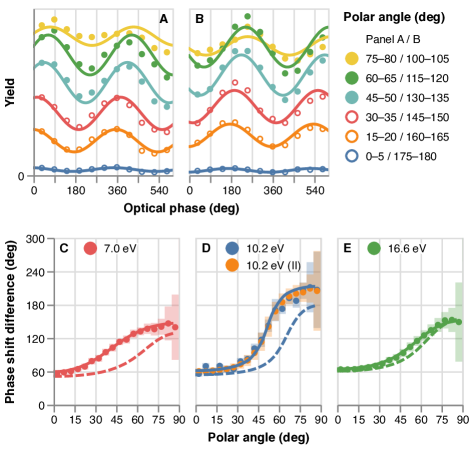
Figure 2:  Upper panels: typical photoelectron yields $I\left(\theta;\phi\right)$ as a function of optical phase $\phi$ at intervals of polar angles $\theta$. The signal was integrated over the $5^{\circ}$ intervals shown on the right. The curves have not been shifted, thus their vertical position reflects directly the value $A_{0}$ in Eq. (4). The photoelectron kinetic energy is 7.0 eV. Circles are experimental results; lines are sinusoidal fits of the experimental results. Lower panels: extracted phase shift differences as a function of the polar angles, for four data sets and three photoelectron kinetic energies: left (C): 7.0 eV; middle (D): 10.2 eV; right (E): 16.6 eV. Circles are experimental results; shaded areas show their uncertainties. Dashed lines: perturbation theory; solid lines: real time ab initio theory. Note that the curves in panels A and B oscillate in antiphase, because they correspond to emission directions on opposite sides of the photon propagation direction.

Figure 3 shows the theoretical dependence of $\Delta\tilde{\eta}\left(\theta\right)$ on electron kinetic energy and polar angle $\theta$, calculated using perturbation theory. There is a single-photon $2p\rightarrow 3s$ resonance of the fundamental wavelength at 16.7 eV photon energy (12 eV kinetic energy for the two-photon/second harmonic). The behavior of $\Delta\tilde{\eta}$ in the region of the resonance is complicated: we can clearly see that $\Delta\tilde{\eta}\left(\theta\right)$ at $\theta\sim 90^{\circ}$ increases near the resonance around 12 eV and then returns to a value similar to that at $\sim 7$ eV. This indicates that the large phase shift difference observed at 10.2 eV in Fig. 2D is due to the influence of the resonance at 12.0 eV Banerjee et al. (2019); Cirelli et al. (2018), and suggests that future experiments should explore this region in fine detail, to observe the predicted rapid changes in $\Delta\tilde{\eta}$. Both theories reproduce this behavior well, with the time-dependent ab initio method exhibiting excellent agreement, validating the present experimental method.

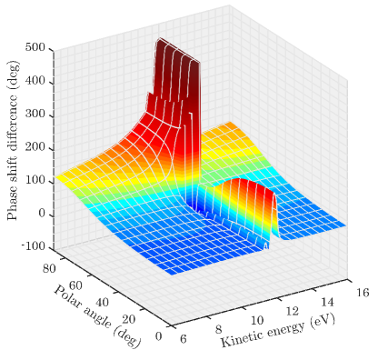
Figure 3:   Phase shift differences $\Delta\tilde{\eta}$ of two-photon ionization relative to single-photon ionization, calculated by perturbation theory, as a function of the polar angle $\theta$ and photoelectron kinetic energy. The large variation near 12.0 eV kinetic energy is due to the $2p\rightarrow 3s$ resonance.

We show in Appendix A that the method is independent of the relative intensities of the fundamental and second harmonic radiation, see Eqs. (A5) to (A9). This is a considerable advantage from an experimental point of view, as it is not necessary to measure precisely the intensity and focal spot shape. Furthermore, there are no effects due to volume averaging over the Gaussian spot profile, or over the duration of the pulses. We verified this experimentally for the kinetic energy of 16.6 eV, Fig. 2D, where the ratio of ionization rates was 1:4 (rather than 1:2 used for the other energies), and the experiment and theory agree well.

VI Discussion

In this section we elucidate the relationship of our data, i.e. photoelectron angular distributions created by collinearly polarized biharmonics, to time-delay studies described in the introduction. We limit ourselves to the case where any discrete state in the continuum (autoionizing state) or in the discrete spectrum lies outside the bandwidth of the pulses ($<$0.02 eV in the present case). These conditions are well fulfilled in our experiments. The resonant case has been discussed elsewhere Argenti et al. (2017).

We first consider the simple situation of photoionization from a spherically symmetric orbital $s$. The present method can be extended straightforwardly to inner shell ionization of atoms, such as $1s^{2}$ of Ne. Single-photon ionization leads to a continuum state with angular momentum $p$, while two-photon ionization leads to two final quantum states $s$ and $d$. Then the PAD $I_{e}(\theta)$ is described by

$$I_{e}(\theta) =\left|c_{s}e^{i\eta_{s}}Y_{00}(\theta,\varphi)+c_{p}e^{i(\eta_{p}+\phi)}Y_{10}(\theta,\varphi)+c_{d}e^{i\eta_{d}}Y_{20}(\theta,\varphi)\right|^{2}\,,$$ (18)

where $c_{s}$, $c_{p}$, and $c_{d}$ are real-valued partial-wave amplitudes and $\eta_{s}$, $\eta_{p}$, and $\eta_{d}$ are the corresponding arguments. $I_{e}(\theta)$ can also be expressed as

$$I_{e}(\theta)=\left(c_{s}^{2}+c_{p}^{2}+c_{d}^{2}\right)\left[1+\sum_{l=1}^{4}\beta_{l}P_{l}(\cos\theta)\right]\,,$$ (19)

where $\ P_{l}(\cos\theta)$ are the Legendre polynomials describing the angular distributions and $\beta_{l}$ are the corresponding asymmetry parameters. After some algebra, we have Di Fraia et al. (2019)

$$\beta_{3} = \frac{6\sqrt{15}c_{d}c_{p}\cos{\left(-\eta_{d}+\eta_{p}+\phi\right)}}{5\left(c_{d}^{2}+{c_{p}}^{2}+c_{s}^{2}\right)}\equiv\left[\beta_{3}\right]_{0}\cos\left(\phi-(\eta_{d}-\eta_{p})\right)\,,$$ (20)

$$\beta_{1}-\frac{2}{3}\beta_{3} = \frac{2\sqrt{3}c_{p}c_{s}\cos{\left(\eta_{p}-\eta_{s}+\phi\right)}}{c_{d}^{2}+{c_{p}}^{2}+c_{s}^{2}}\equiv\left[\beta_{1}-\frac{2}{3}\beta_{3}\right]_{0}\cos{\left(\phi-(\eta_{s}-\eta_{p})\right)}\;,$$ (21)

where $[\beta_{3}]_{0}$ and $[\beta_{1}-\frac{2}{3}\beta_{3}]_{0}$ are constants. Thus, if we record PADs as a function of $\phi$ and extract $\beta_{l}$ ($l=1$ to 4), we can directly read off $\eta_{d}-\eta_{p}$ and $\eta_{s}-\eta_{p}$ from the oscillations of $\beta_{3}$ and $\beta_{1}-\frac{2}{3}\beta_{3}$ using Eqs. (20) and (21). Let us recall that the Wigner delay of each partial wave, $\tau_{l}$, corresponds to the energy derivative of the argument of the amplitude (note that $Y_{l0}(\theta,\varphi)$ are real), $\tau_{l}(\epsilon)=\frac{{d\eta}_{l}(\epsilon)}{d\epsilon}$ Wigner (1955). By measuring $\eta_{d}-\eta_{p}$ and $\eta_{s}-\eta_{p}$ as a function of energy, one can take the energy derivative and obtain the Wigner delay differences $\tau_{l}(\epsilon)-\tau_{p}(\epsilon)$ with $l=s$ and $d$. In simple models, like the Hartree-Fock approximation, $\frac{{d\eta}_{l}(\epsilon)}{d\epsilon}=\frac{{d\delta}_{l}(\epsilon)}{d\epsilon}$, where $\delta_{l}(\epsilon)$ is the scattering phase, while in more complicated cases, an extra energy dependent phase may be acquired by the partial amplitude Wätzel et al. (2015).

We now group the $s$ and $d$ waves as a two-photon-ionization wave packet. Then the photoelectron wave packet in a given direction $\theta$ sufficiently far from the nucleus, and the corresponding PAD are expressed as Eqs. (3) and (4), respectively. The energy derivative of $\Delta\eta\left(\theta\right)\equiv\eta_{\omega}(\theta)-\eta_{2\omega}(\theta)$ is a difference between the group delays of the two wave packets, generated by two- and single-photon ionization, respectively. In the original photoemission delay experiment Schultze et al. (2010) with attosecond streaking, for example, Ne $2s$ and $2p$ electrons were ionized by an attosecond pulse to different final kinetic energies. As a result, the more energetic photoelectron from $2p$ arrived at the detector much earlier than that from $2s$, regardless of the measured delay. The situation is similar for subsequent measurements using streaking and RABBITT. In great contrast, in the present case, both single- and two-photon ionization result in the same photoelectron energy. Therefore, the single- and two-photon-ionization wave packets actually reach a given distance with a relative (group) delay given by $\frac{\partial\Delta\eta}{\partial\epsilon}$.

By comparing Eqs. (4) and (18), we can describe the phase factor $e^{i\Delta\eta\left(\theta\right)}$ with $\Delta\eta\left(\theta\right)\equiv\eta_{\omega}(\theta)-\eta_{2\omega}(\theta)$ being the angle-resolved phase difference between the two-photon and single-photon ionization amplitudes as,

$$A(\theta)e^{i\Delta\eta(\theta)}=2c_{p}Y_{10}(\theta,\varphi)\left[c_{d}Y_{20}(\theta,\varphi)\,e^{i(\eta_{d}-\eta_{p})}+c_{s}Y_{00}(\theta)\,e^{i(\eta_{s}-\eta_{p})}\right].$$ (22)

Thus, the phase factor $e^{i\Delta\eta\left(\theta\right)}$ is the coherent (i.e., with respect to amplitudes) average of $e^{i(\eta_{d}-\eta_{p})}$ ($d$-$p$ interference) and $e^{i(\eta_{s}-\eta_{p})}$ ($s$-$p$ interference) with the relative weight,

$$W(\theta)=B\,g(\theta),\qquad B=\frac{c_{d}}{c_{s}},\qquad g(\theta)=\frac{Y_{20}(\theta,\varphi)}{Y_{00}(\theta,\varphi)}=\frac{\sqrt{5}}{4}\left[3\cos(2\theta)+1\right]\,.$$ (23)

In other words, $\Delta\eta\left(\theta\right)$ can be regarded as a $vectorial$ average of $\eta_{s}-\eta_{p}$ and $\eta_{d}-\eta_{p}$ with the relative weight $W(\theta)$. Equivalently, $\Delta\eta(\theta)$ may be presented as

$$\tan\Delta\eta\left(\theta\right)=\frac{\cos(\eta_{s}-\eta_{p})+W(\theta)\,\cos(\eta_{d}-\eta_{p})}{\sin(\eta_{s}-\eta_{p})+W(\theta)\,\sin(\eta_{d}-\eta_{p})}\,.$$ (24)

The energy derivative of $\Delta\eta(\theta)$ does not give us additional information about the photoionization amplitudes, but provides us with the group delay and may enhance the sensitivity to the energy-dependent behavior of the two-photon ionization amplitudes, as described below.

Note two important characteristics of $\Delta\eta\left(\theta\right)$: (i) $\Delta\eta\left(\theta\right)$ exhibits a quasi-cosine shape, and monotonic dependence on $\theta$ due to the geometric factor $g(\theta)$ (see Fig. 2(c)-(e) and Appendix A) and (ii) $\Delta\eta\left(\theta\right)$ is sensitive to the two-photon ionization dynamics due to the dynamical factor $B$. For example, if the two-photon pathways are close to an intermediate discrete resonance (but still well outside the bandwidth), the group delay difference $\frac{\partial\Delta\eta}{\partial\epsilon}(\theta)$ is sensitive to it through rapid change in $B$, while $\frac{d\eta_{s}}{d\epsilon},\frac{d\eta_{p}}{d\epsilon}$, and $\frac{d\eta_{d}}{d\epsilon}$ are small individually, as can be seen in Fig. 3.

We now turn to photoionization from a $p$ orbital, which includes the present case of Ne 2$p$ ionization, and is more complicated. The complexity arises from two sources. We have three incoherent contributions from $m=0$ and $\pm 1$ for the magnetic sublevels of the remaining ion core Ne⁺ and four contributions of partial waves, $s$, $p$, $d$, and $f$ in the photoelectron wavepacket. Detailed derivations of the equations describing the PADs are given in Appendix A and here we describe only the results relevant to the present discussion. For $m=\pm 1$, we have a pair of two-photon pathways via $d$ intermediate states, i.e., $p\rightarrow d\rightarrow p$ and $p\rightarrow d\rightarrow f$, together with the single-photon pathway $p\rightarrow d$. Thus, only three partial waves are involved and therefore a discussion similar to that above for $s$ ionization holds.

For $m=0$, we have two-photon pathways via $s$ and $d$ intermediate states, leading to $p$ and $f$ final states, together with single-photon ionization that leads to $s$ and $d$ final states. Thus, there are four partial waves involved. Although we can derive equations similar to Eqs. (20) and  (21) (see Eqs. (38)-(41)), what we can extract from the measurement is only a vectorial average of phase differences $\eta_{l}-\eta_{l^{\prime}}$ between even and odd different partial waves $l$, $l^{\prime}$. We can define the angle-resolved phase difference $\Delta\eta_{m}(\theta)$ for each $m$ (see Eq. (5)), which is also a vectorial average of $\eta_{l}-\eta_{l^{\prime}}$. Similar to ionization from the $s$ state, the energy derivative of $\Delta\eta_{m}(\theta)$ may be regarded as an angle-resolved group delay between single- and two-photon wave packets for each $m$.

In the experiment, we measured an (incoherently) weighted average $\Delta\tilde{\eta}$ of angle-resolved phase differences $\Delta\eta_{m}$ of different $m$ as defined in Eqs. (5) and (6). One can introduce the energy derivative of the weighted average phase difference $\Delta\tilde{\eta}(\theta)$, and may call it generalized delay, but this definition of time delay is different from that commonly employed for the time delay of an incoherent sum of wavepackets. Usually the phase of each wavepacket is first differentiated with respect to energy and then averaged over $m$ Smith (1960), while in this study, $\frac{d\Delta\tilde{\eta}}{d\epsilon}(\theta)$ first averages the wavepacket phase over $m$ and then differentiates it with respect to the photoelectron energy.

VII Summary and outlook

In this work we have described a new method to determine angle-resolved relative phase between single- and two-photon ionization amplitudes, and used it to measure the $2p$ photoionization of Ne. Our approach allows us to explore the phase difference between different ionization pathways, e.g., those of odd and even parities, with the same photoelectron energy.

The method is based on FEL radiation, so that it can be extended to shorter wavelengths, eventually to inner shells, which lie in a wavelength region where optical lasers have reduced pulse energy. This is an important addition to the armoury of techniques available to attosecond science and gives access to the phase difference between single- (odd parity) and two-photon (even parity) transition amplitudes, or the energy variation of the phase of two-photon ionization amplitudes affected by the intermediate resonances, as seen in the Ne $2p$ photoionization. For $ns^{2}$ subshells of atoms, e.g., $1s^{2}$ of He, $1s^{2}$ and $2s^{2}$ of Ne, etc. in particular, one can extract the eigenphase differences for $s$, $p$, and $d$ partial waves of electron-ion scattering, and their energy derivatives correspond to the Wigner delay difference of the partial waves. This method is also applicable to molecules.

While it does not yet appear to be feasible with present HHG sources, it may become possible in the future, but there are many technical challenges. Since HHG sources produce a frequency comb, the chief technical challenges are to filter the beam to achieve bichromatic spectral purity, maintain attosecond temporal resolution, and provide enough pulse energy at the fundamental wavelength to initiate two-photon ionization. Furthermore, HHG sources have not yet demonstrated the level of phase control which we have at our disposal. Given the rapid progress in HHG sources, these conditions may eventually be met, in which case our method will become more widely accessible.

The information obtained by this method is complementary to that of streaking and RABBITT methods, in the sense that different phase differences are measured. We have directly measured the angle-resolved average phase difference $\Delta\tilde{\eta}\left(\theta\right)$ of two-photon amplitude relative to the single-photon ionization amplitude. The basic physics giving rise to its angular dependence is related to interference between photoelectron waves emitted in one- and two-photon ionization, consisting of partial photoelectron waves with opposite parities. We have shown that the overall shape of $\Delta\tilde{\eta}\left(\theta\right)$ versus angle can be understood qualitatively.

Appendix A Perturbation theory. Derivation of equations in the independent particle model

In addition to the approximations described in Section IV.3 (the dipole approximation, the validity of the lowest nonvanishing order perturbation theory), here we add the LS-coupling approximation within the independent particle model. The photoelectron angular distribution $I(\theta;\phi)$ of a Ne 2$p$ electron can be derived by standard methods Amusia (1990) in the form

$$I(\theta;\phi)=I_{0}\sum_{m=0,\pm 1}\left|\sum_{\xi}C^{m}_{\xi}(\phi)Y_{\ell_{\xi}m}(\theta,\varphi)\right|^{2}\,,$$ (25)

where $m$ is the magnetic quantum number of the initial $2p$ electron, $Y_{\ell m}(\theta,\varphi)$ is a spherical harmonic in the Condon-Shortley phase convention, $I_{0}$ is a normalization factor irrelevant to further discussion; note that the dependence on $\varphi$ cancels out. The complex coefficients $C^{m}_{\xi}(\phi)$ depend on ionization amplitudes, and the index $\xi$ denotes the ionization path. For single-photon ionization $\xi=\ell_{\xi}$, where $\ell_{\xi}$ is the orbital momentum of the photoelectron with possible values $\ell_{\xi}=s,\,d$. For two-photon ionization $\xi=\{\ell_{\xi},\ell^{\prime}_{\xi}\}$, where $\ell^{\prime}_{\xi}$ is the orbital momentum of the virtual intermediate state, with possible combinations $\xi=ps,\,pd,\,fd$.

After applying the Wigner-Eckart theorem Varshalovich et al. (1988) to factor out the dependence on the projection $m$, the coefficients $C^{m}_{\xi}(\phi)$ may be expressed as (for brevity, we omit the argument $\phi$ when writing the coefficients):

$$C_{s}^{0}=-\frac{1}{\sqrt{3}}D_{s}\,e^{i\phi},\;\;C_{d}^{0}=\sqrt{\frac{2}{15}}D_{d}\,e^{i\phi},\;\;C_{d}^{\pm 1}=\frac{1}{\sqrt{10}}D_{d}\,e^{i\phi},$$ (26)

$$C^{0}_{ps}=-\frac{1}{3}D_{ps},\;\;C^{\pm 1}_{ps}=0,$$

$$C^{0}_{pd}=-\frac{2}{15}D_{pd},\;\;C^{\pm 1}_{pd}=-\frac{1}{10}D_{pd},$$

$$C^{0}_{fd}=\frac{\sqrt{2}}{5\sqrt{7}}D_{fd},\;\;C^{\pm 1}_{fd}=\frac{2}{5\sqrt{21}}D_{fd}.$$ (27)

Here

$$D_{\xi}=d_{\xi}\,e^{i\eta_{\xi}}$$ (28)

are complex reduced matrix elements, independent of $m$, with magnitude $d_{\xi}=\left|D_{\xi}\right|$ and phase $\eta_{\xi}$. Note that one- (first order) and two-photon (second order) matrix elements (28), both marked by a single index $\xi$, are respectively proportional to the square root of intensity, and to intensity, of the associated field.

Equation (25) can be readily cast into the form (4), where

$$A_{0} = \frac{I_{0}}{4\pi}\sum_{\lambda=0,2,4}Z_{\lambda}P_{\lambda}(\cos\theta),$$ (29)

$$A = \frac{I_{0}}{4\pi}\,N\,,$$ (30)

$$\cos\Delta\tilde{\eta} = N^{-1}\sum_{\lambda=1,3}{\rm Re}\,Z^{\prime}_{\lambda}P_{\lambda}(\cos\theta)\,,$$ (31)

$$\sin\Delta\tilde{\eta} = N^{-1}\sum_{\lambda=1,3}{\rm Im}\,Z^{\prime}_{\lambda}P_{\lambda}(\cos\theta)\,,$$ (32)

$$N = \left|\sum_{\lambda=1,3}Z^{\prime}_{\lambda}P_{\lambda}(\cos\theta)\right|\,,$$ (33)

$$Z_{\lambda}=\sum_{\begin{subarray}{c}m=0,\pm 1\\ \xi=s,d,ps,pd,fd\\ \bar{\xi}=s,d,ps,pd,fd\end{subarray}}(-1)^{m}C_{\xi}^{m}C_{\bar{\xi}}^{m\ast}\sqrt{(2\ell_{\xi}+1)(2\ell_{\bar{\xi}}+1)}\mbox{$\left(\ell_{\xi}m,\ell_{\bar{\xi}}-m\,|\,\lambda 0\right)$}\mbox{$\left(\ell_{\xi}0,\ell_{\bar{\xi}}0\,|\,\lambda 0\right)$}\,,$$ (34)

where $\left(j_{1}m_{1},j_{2}m_{2}\,|\,jm\right)$ are Clebsch-Gordan coefficients Varshalovich et al. (1988) and $Z^{\prime}_{\lambda}=Z_{\lambda}|_{\phi=0}$. In particular

$$Z_{0}=\frac{1}{30}\Big{[}10(d_{d}^{2}+d_{s}^{2})+\frac{4}{5}d_{fd}^{2}+\frac{17}{15}d_{pd}^{2}+\frac{10}{3}d_{ps}^{2}+\frac{8}{3}d_{pd}d_{ps}\cos(\eta_{pd}-\eta_{ps})\Big{]}.$$ (35)

Equations (26)-(34) define $\Delta\tilde{\eta}$, provided the reduced matrix elements (28) are calculated. The intensities of the fundamental and of the second harmonic are factored out in the coefficients $Z^{\prime}_{\lambda}$, therefore they cancel out in Eqs. (31), (32) and the phases $\Delta\tilde{\eta}$ are independent of the intensities of the harmonics.

Note that the angle-resolved average phase difference $\Delta\tilde{\eta}$ between one- and two-photon ionization implies not less than two ionization channels, which is reflected in the non-vanishing sum over channels in Eq. (34). Therefore $\Delta\tilde{\eta}$ and its energy derivative, or as we called it, generalized delay, is always angle-dependent.

The coefficients (34) are directly related to the anisotropy parameters $\beta_{\lambda}$ in the angular distribution of photoelectrons (25) written in the form

$$I(\theta;\phi)=\frac{W_{0}}{4\pi}\left(1+\sum_{\lambda=1}^{4}\beta_{\lambda}P_{\lambda}(\cos\theta)\right)\,,$$ (36)

where

$$\beta_{\lambda}=\frac{Z_{\lambda}}{Z_{0}}$$ (37)

and $W_{0}=I_{0}Z_{0}$. Substituting Eqs. (34) and (26), (A) into (37) one can express the anisotropy parameters in terms of reduced matrix elements (28):

$$\beta_{1} = \frac{1}{15Z_{0}}\Bigg{[}\frac{12\sqrt{3}}{5}d_{d}d_{fd}\cos(\eta_{fd}-\eta_{d}-\phi)-\,\frac{17\sqrt{2}}{5}d_{d}d_{pd}\cos(\eta_{pd}-\eta_{d}-\phi)$$ (38)

$$-\,4\sqrt{2}\,d_{d}d_{ps}\cos(\eta_{ps}-\eta_{d}-\phi)+4\,d_{s}d_{pd}\cos(\eta_{pd}-\eta_{s}-\phi)$$

$$+\,10\,d_{s}d_{ps}\cos(\eta_{ps}-\eta_{s}-\phi)\Bigg{]},$$

$$\beta_{2} = \frac{1}{210Z_{0}}\Bigg{[}70d_{d}^{2}+\frac{32}{5}\,d_{fd}^{2}+\frac{49}{15}d_{pd}^{2}+\frac{140}{3}d_{ps}^{2}-\,140\sqrt{2}\,d_{d}d_{s}\cos(\eta_{d}-\eta_{s})$$ (39)

$$-\,\frac{48\sqrt{6}}{5}d_{fd}d_{pd}\cos(\eta_{fd}-\eta_{pd})-12\sqrt{6}\,d_{fd}d_{ps}\cos(\eta_{fd}-\eta_{ps})$$

$$+\,\frac{112}{3}d_{pd}d_{ps}\cos(\eta_{pd}-\eta_{ps})\Bigg{]},$$

$$\beta_{3} = \frac{1}{30Z_{0}}\Bigg{[}\frac{16\sqrt{3}}{5}d_{d}d_{fd}\cos(\eta_{fd}-\eta_{d}-\phi)-\frac{6\sqrt{2}}{5}d_{d}d_{pd}\cos(\eta_{pd}-\eta_{d}-\phi)$$ (40)

$$-\,12\sqrt{2}\,d_{d}d_{ps}\cos(\eta_{ps}-\eta_{d}-\phi)-4\sqrt{6}\,d_{s}d_{fd}\cos(\eta_{fd}-\eta_{s}-\phi)\Bigg{]},$$

$$\beta_{4} = \frac{4}{35Z_{0}}\left[\frac{1}{5}d_{fd}^{2}-\frac{\sqrt{2}}{5\sqrt{3}}d_{fd}d_{pd}\cos(\eta_{fd}-\eta_{pd})-\frac{2\sqrt{2}}{\sqrt{3}}d_{fd}d_{ps}\cos(\eta_{fd}-\eta_{ps})\right]\,.$$ (41)

The terms containing cosine functions describe the contribution from the phase difference between two-photon and single-photon ionization channels. For example, $\cos(\eta_{fd}-\eta_{d}-\phi)$ in Eq. (38) corresponds to the phase difference between $p\to d\to f$ two-photon-ionization (TPI) and $p\to d$ single-photon-ionization (SPI) channels as well as the relative phase of the harmonics $\phi$. Note that $\beta_{2}$ and $\beta_{4}$ do not depend on $\phi$.

It immediately follows from Eqs. (31), (32)

$$\tan\Delta\tilde{\eta}=\frac{{\rm Im}Z^{\prime}_{1}P_{1}(\cos\theta)+{\rm Im}Z^{\prime}_{3}P_{3}(\cos\theta)}{{\rm Re}Z^{\prime}_{1}P_{1}(\cos\theta)+{\rm Re}Z^{\prime}_{3}P_{3}(\cos\theta)}=\frac{{\rm Im}Z^{\prime}_{1}+f(\theta){\rm Im}Z^{\prime}_{3}}{{\rm Re}Z^{\prime}_{1}+f(\theta){\rm ReZ^{\prime}_{3}}}\,,$$ (42)

where the function $f(\theta)=\frac{1}{4}\left[5\cos(2\theta)-1\right]$ is displayed in Fig. 4.

Figure 4: Plot of $(5\cos 2\theta-1)/4$ as a function of $\theta$.

This qualitatively explains the quasi-cosine shape, and monotonic dependence of $\Delta\tilde{\eta}$ on $\theta$ (Fig. 2 C-E). $Z^{\prime}_{\lambda}$ are independent of $\phi$, so that $\Delta\tilde{\eta}$ and the generalized delay are independent of the relative phase between the harmonics.

The functional form of Eq. (42) is very general and valid, within the perturbation theory and the dipole approximation, for randomly oriented atoms and molecules, provided corresponding expressions for the coefficients $Z_{\lambda}$ in terms of the ionization amplitudes are used. Moreover, it holds for circularly polarized collinear photon beams (except for chiral targets), provided the angle $\theta$ is measured from the direction of the beam propagation.

Expression (42) may be written in an equivalent form in terms of $\theta$-independent “average partial” TPI-SPI phase differences $\Delta\tilde{\eta}_{\lambda}$ ($\lambda=1,\,3$). Indeed, we can write Eq. (36) explicitly in the form [see Eqs. (5) and  (6)]

$$4\pi W_{0}^{-1}I(\theta;\phi) = [1+\beta_{2}P_{2}(\cos\theta)+\beta_{4}P_{4}(\cos\theta)]$$ (43)

$$~{}~{}~{}~{}~{}~{}~{}+[\gamma_{1}\cos(\phi-\Delta\tilde{\eta}_{1})P_{1}(\cos\theta)+\gamma_{3}\cos(\phi-\Delta\tilde{\eta}_{3})P_{3}(\cos\theta)]$$

$$= A_{0}(\theta)+A(\theta)\cos[\phi-\Delta\tilde{\eta}\left(\theta\right)]\,.$$

Here the prefactors $\gamma_{1}$, $\gamma_{3}$ and phases $\Delta\tilde{\eta}_{1}$, $\Delta\tilde{\eta}_{3}$ are independent of $\theta$ and $\phi$. It follows from (43) that $\Delta\tilde{\eta}\left(\theta\right)$ can be viewed as a “vectorial” average of $\Delta\tilde{\eta}_{1}$ and $\Delta\tilde{\eta}_{3}$ with weights $\gamma_{1}P_{1}(\cos\theta)$ and $\gamma_{3}P_{3}(\cos\theta)$, in the sense that $\Delta\tilde{\eta}\left(\theta\right)$ is the directional angle of vector

$$\left(\gamma_{1}P_{1}(\cos\theta)\cos\Delta\tilde{\eta}_{1}+\gamma_{3}P_{3}(\cos\theta)\cos\Delta\tilde{\eta}_{3},\gamma_{1}P_{1}(\cos\theta)\sin\Delta\tilde{\eta}_{1}+\gamma_{3}P_{3}(\cos\theta)\sin\Delta\tilde{\eta}_{3}\right),$$ (44)

satisfying,

$$\tan\Delta\tilde{\eta}\left(\theta\right)=\frac{\gamma_{1}P_{1}(\cos\theta)\sin\Delta\tilde{\eta}_{1}+\gamma_{3}P_{3}(\cos\theta)\sin\Delta\tilde{\eta}_{3}}{\gamma_{1}P_{1}(\cos\theta)\cos\Delta\tilde{\eta}_{1}+\gamma_{3}P_{3}(\cos\theta)\cos\Delta\tilde{\eta}_{3}}.$$ (45)

There are simple relations between the “average partial” TPI-SPI phase differences and parameters of Eq. (42):

$$\sin\Delta\tilde{\eta}_{\lambda}=\frac{{\rm Im}\,Z^{\prime}_{\lambda}}{\left|Z^{\prime}_{\lambda}\right|},\quad\cos\Delta\tilde{\eta}_{\lambda}=\frac{{\rm Re}\,Z^{\prime}_{\lambda}}{\left|Z^{\prime}_{\lambda}\right|},\quad(\lambda=1,\,3)$$ (46)

and also

$$\gamma_{1}=\left|Z^{\prime}_{3}\right|^{-1},\quad\gamma_{3}=\left|Z^{\prime}_{1}\right|^{-1}\,.$$ (47)

As stated above, we can use the fact that the parity of Legendre Polynomials obeys $P_{n}(-x)=(-1)^{n}P_{n}(x)$, so that the vector defined by Eq. (44) changes sign upon performing the substitution $\theta\rightarrow\pi-\theta$, i.e., the two halves of the VMI image oscillate in antiphase: $\Delta\tilde{\eta}\left(\theta\right)=\Delta\tilde{\eta}\left(\pi-\theta\right)+\pi$.

References

- Krausz and Ivanov (2009) F. Krausz and M. Ivanov, Attosecond physics, Rev. Mod. Phys. 81, 163 (2009).
- Wigner (1955) E. P. Wigner, Lower limit for the energy derivative of the scattering phase shift, Phys. Rev. 98, 145 (1955).
- Pabst and Dahlström (2016) S. Pabst and J. M. Dahlström, Eliminating the dipole phase in attosecond pulse characterization using Rydberg wave packets, Phys. Rev. A 94, 013411 (2016).
- Klünder et al. (2011) K. Klünder, J. M. Dahlström, M. Gisselbrecht, T. Fordell, M. Swoboda, D. Guénot, P. Johnsson, J. Caillat, J. Mauritsson, A. Maquet, R. Taïeb, and A. L’Huillier, Probing single-photon ionization on the attosecond time scale, Phys. Rev. Lett. 106, 143002 (2011).
- Guénot et al. (2014) D. Guénot, D. Kroon, E. Balogh, E. W. Larsen, M. Kotur, M. Miranda, T. Fordell, P. Johnsson, J. Mauritsson, M. Gisselbrecht, K. Varjú, C. L. Arnold, T. Carette, A. S. Kheifets, E. Lindroth, A. L’Huillier, and J. M. Dahlström, Measurements of relative photoemission time delays in noble gas atoms, J. Phys. B 47, 245602 (2014).
- Guénot et al. (2012) D. Guénot, K. Klünder, C. L. Arnold, D. Kroon, J. M. Dahlström, M. Miranda, T. Fordell, M. Gisselbrecht, P. Johnsson, J. Mauritsson, E. Lindroth, A. Maquet, R. Taïeb, A. L’Huillier, and A. S. Kheifets, Photoemission-time-delay measurements and calculations close to the 3s-ionization-cross-section minimum in Ar, Phys. Rev. A 85, 053424 (2012).
- Palatchi et al. (2014) C. Palatchi, J. M. Dahlström, A. S. Kheifets, I. A. Ivanov, D. M. Canaday, P. Agostini, and L. F. DiMauro, Atomic delay in helium, neon, argon and krypton, J. Phys. B 47, 245003 (2014).
- Kheifets (2013) A. S. Kheifets, Time delay in valence-shell photoionization of noble-gas atoms, Phys. Rev. A 87, 063404 (2013).
- Saha et al. (2014) S. Saha, A. Mandal, J. Jose, H. R. Varma, P. C. Deshmukh, A. S. Kheifets, V. K. Dolmatov, and S. T. Manson, Relativistic effects in photoionization time delay near the Cooper minimum of noble-gas atoms, Phys. Rev. A 90, 053406 (2014).
- Argenti et al. (2017) L. Argenti, A. Jiménez-Galán, J. Caillat, R. Taïeb, A. Maquet, and F. Martín, Control of photoemission delay in resonant two-photon transitions, Phys. Rev. A 95, 043426 (2017).
- Busto et al. (2019) D. Busto, J. Vinbladh, S. Zhong, M. Isinger, S. Nandi, S. Maclot, P. Johnsson, M. Gisselbrecht, A. L’Huillier, E. Lindroth, and J. M. Dahlström, Fano’s Propensity Rule in Angle-Resolved Attosecond Pump-Probe Photoionization, Phys. Rev. Lett. 123, 133201 (2019).
- Vos et al. (2018) J. Vos, L. Cattaneo, S. L. Patchkovskii, T. Zimmermann, C. Cirelli, M. Lucchini, A. Kheifets, A. S. Landsman, and U. Keller, Orientation-dependent stereo Wigner time delay and electron localization in a small molecule, Science 360, 1326 (2018).
- Azoury et al. (2019a) D. Azoury, O. Kneller, M. Krüger, B. D. Bruner, O. Cohen, Y. Mairesse, and N. Dudovich, Interferometric attosecond lock-in measurement of extreme-ultraviolet circular dichroism, Nat. Photonics 13, 198 (2019a).
- Fuchs et al. (2020) J. Fuchs, N. Douguet, S. Donsa, F. Martin, J. Burgdörfer, L. Argenti, L. Cattaneo, and U. Keller, Time delays from one-photon transitions in the continuum, Optica 7, 154 (2020).
- Ossiander et al. (2017) M. Ossiander, F. Siegrist, V. Shirvanyan, R. Pazourek, A. Sommer, T. Latka, A. Guggenmos, S. Nagele, J. Feist, J. Burgdörfer, R. Kienberger, and M. Schultze, Attosecond correlation dynamics, Nature Physics 13, 280 (2017).
- Schultze et al. (2010) M. Schultze, M. Fieß, N. Karpowicz, J. Gagnon, M. Korbman, M. Hofstetter, S. Neppl, A. L. Cavalieri, Y. Komninos, T. Mercouris, C. A. Nicolaides, R. Pazourek, S. Nagele, J. Feist, J. Burgdörfer, A. M. Azzeer, R. Ernstorfer, R. Kienberger, U. Kleineberg, E. Goulielmakis, F. Krausz, and V. S. Yakovlev, Delay in photoemission, Science 328, 1658 (2010).
- Eckle et al. (2008a) P. Eckle, A. N. Pfeiffer, C. Cirelli, A. Staudte, R. Dörner, H. G. Muller, M. Büttiker, and U. Keller, Attosecond Ionization and Tunneling Delay Time Measurements in Helium, Science 322, 1525 (2008a).
- Eckle et al. (2008b) P. Eckle, M. Smolarski, P. Schlup, J. Biegert, A. Staudte, M. Schöffler, H. G. Muller, R. Dörner, and U. Keller, Attosecond angular streaking, Nat. Phys. 4, 565 (2008b).
- Pfeiffer et al. (2012) A. N. Pfeiffer, C. Cirelli, M. Smolarski, D. Dimitrovski, M. Abu-samha, L. B. Madsen, and U. Keller, Attoclock reveals natural coordinates of the laser-induced tunnelling current flow in atoms, Nat. Phys. 8, 76 (2012).
- Pfeiffer et al. (2011) A. N. Pfeiffer, C. Cirelli, M. Smolarski, R. Dörner, and U. Keller, Timing the release in sequential double ionization, Nat. Phys. 7, 428 (2011).
- Paul et al. (2001) P. M. Paul, E. S. Toma, P. Breger, G. Mullot, F. Augé, P. Balcou, H. G. Muller, and P. Agostini, Observation of a train of attosecond pulses from high harmonic generation, Science 292, 1689 (2001).
- Loriot et al. (2017) V. Loriot, A. Marciniak, G. Karras, B. Schindler, G. Renois-Predelus, I. Compagnon, B. Concina, R. Brédy, G. Celep, C. Bordas, E. Constant, and F. Lépine, Angularly resolved RABBITT using a second harmonic pulse, J. Opt. 19, 114003 (2017).
- Azoury et al. (2019b) D. Azoury, O. Kneller, S. Rosen, B. D. Bruner, A. Clergerie, Y. Mairesse, B. Fabre, B. Pons, N. Dudovich, and M. Krüger, Electronic wavefunctions probed by all-optical attosecond interferometry, Nat. Photonics 13, 54 (2019b).
- Villeneuve et al. (2017) D. M. Villeneuve, P. Hockett, M. J. J. Vrakking, and H. Niikura, Coherent imaging of an attosecond electron wave packet, Science 356, 1150 (2017).
- Donsa et al. (2019) S. Donsa, N. Douguet, J. Burgdörfer, I. Březinová, and L. Argenti, Circular holographic ionization-phase meter, Phys. Rev. Lett. 123, 133203 (2019).
- Dahlström and Lindroth (2014) J. M. Dahlström and E. Lindroth, Study of attosecond delays using perturbation diagrams and exterior complex scaling, J. Phys. B 47, 124012 (2014).
- Wätzel et al. (2015) J. Wätzel, A. S. Moskalenko, Y. Pavlyukh, and J. Berakdar, Angular resolved time delay in photoemission, J. Phys. B 48, 025602 (2015).
- Heuser et al. (2016) S. Heuser, Á. J. Galán, C. Cirelli, C. Marante, R. Sabbar, Mazyarand Boge, M. Lucchini, L. Gallmann, I. Ivanov, A. S. Kheifets, J. M. J. Dahlström, E. Lindroth, L. Argenti, F. Martín, and U. Keller, Angular dependence of photoemission time delay in helium, Phys. Rev. A 94, 063409 (2016).
- Mandal et al. (2017) A. Mandal, P. C. Deshmukh, A. S. Kheifets, V. K. Dolmatov, and S. T. Manson, Angle-resolved Wigner time delay in atomic photoionization: The 4d subshell of free and confined Xe, Phys. Rev. A 96, 053407 (2017).
- Ivanov and Kheifets (2017) I. A. Ivanov and A. S. Kheifets, Angle-dependent time delay in two-color XUV+IR photoemission of He and Ne, Phys. Rev. A 96, 013408 (2017).
- Bray et al. (2018) A. W. Bray, F. Naseem, and A. S. Kheifets, Photoionization of Xe and Xe and Xe@C60 from the 4d shell in RABBITT fields, Phys. Rev. A 98, 043427 (2018).
- Banerjee et al. (2019) S. Banerjee, P. C. Deshmukh, V. K. Dolmatov, S. T. Manson, and A. S. Kheifets, Strong dependence of photoionization time delay on energy and angle in the neighborhood of Fano resonances, Phys. Rev. A 99, 013416 (2019).
- Cirelli et al. (2018) C. Cirelli, C. Marante, S. Heuser, C. L. M. Petersson, Á. J. Galán, L. Argenti, S. Zhong, D. Busto, M. Isinger, S. Nandi, S. Maclot, L. Rading, P. Johnsson, M. Gisselbrecht, M. Lucchini, L. Gallmann, J. M. Dahlström, E. Lindroth, A. L’Huillier, F. Martín, and U. Keller, Anisotropic photoemission time delays close to a Fano resonance, Nat. Comm. 9, 955 (2018).
- Shapiro and Brumer (2003) M. Shapiro and P. Brumer, Principles of the Quantum Control of Molecular Processes (Wiley-Interscience, Hoboken, N.J., 2003).
- Prince et al. (2016) K. C. Prince, E. Allaria, C. Callegari, R. Cucini, G. De Ninno, S. Di Mitri, B. Diviacco, E. Ferrari, P. Finetti, D. Gauthier, L. Giannessi, N. Mahne, G. Penco, O. Plekan, L. Raimondi, P. Rebernik, E. Roussel, C. Svetina, M. Trovò, M. Zangrando, M. Negro, P. Carpeggiani, M. Reduzzi, G. Sansone, A. N. Grum-Grzhimailo, E. V. Gryzlova, S. I. Strakhova, K. Bartschat, N. Douguet, J. Venzke, D. Iablonskyi, Y. Kumagai, T. Takanashi, K. Ueda, A. Fischer, M. Coreno, F. Stienkemeier, Y. Ovcharenko, T. Mazza, and M. Meyer, Coherent control with a short-wavelength free-electron laser, Nat. Photonics 10, 176 (2016).
- Lyamayev et al. (2013) V. Lyamayev, Y. Ovcharenko, R. Katzy, M. Devetta, L. Bruder, A. LaForge, M. Mudrich, U. Person, F. Stienkemeier, M. Krikunova, T. Möller, P. Piseri, L. Avaldi, M. Coreno, P. O’Keeffe, P. Bolognesi, M. Alagia, A. Kivimäki, M. D. Fraia, N. B. Brauer, M. Drabbels, T. Mazza, S. Stranges, P. Finetti, C. Grazioli, O. Plekan, R. Richter, K. C. Prince, and C. Callegari, A modular end-station for atomic, molecular, and cluster science at the low density matter beamline of FERMI@Elettra, J. Phys. B 46, 164007 (2013).
- Svetina et al. (2015) C. Svetina, C. Grazioli, N. Mahne, L. Raimondi, C. Fava, M. Zangrando, S. Gerusina, M. Alagia, L. Avaldi, G. Cautero, M. de Simone, M. Devetta, M. Di Fraia, M. Drabbels, V. Feyer, P. Finetti, R. Katzy, A. Kivimäki, V. Lyamayev, T. Mazza, A. Moise, T. Möller, P. O’Keeffe, Y. Ovcharenko, P. Piseri, O. Plekan, K. C. Prince, R. Sergo, F. Stienkemeier, S. Stranges, M. Coreno, and C. Callegari, The Low Density Matter (LDM) beamline at FERMI: optical layout and first commissioning, J. Synchrotron Radiat. 22, 538 (2015).
- Allaria et al. (2015) E. Allaria, L. Badano, S. Bassanese, F. Capotondi, D. Castronovo, P. Cinquegrana, M. B. Danailov, G. D’Auria, A. Demidovich, R. De Monte, G. De Ninno, S. Di Mitri, B. Diviacco, W. M. Fawley, M. Ferianis, E. Ferrari, G. Gaio, D. Gauthier, L. Giannessi, F. Iazzourene, G. Kurdi, N. Mahne, I. Nikolov, F. Parmigiani, G. Penco, L. Raimondi, P. Rebernik, F. Rossi, E. Roussel, C. Scafuri, C. Serpico, P. Sigalotti, C. Spezzani, M. Svandrlik, C. Svetina, M. Trovó, M. Veronese, D. Zangrando, and M. Zangrando, The FERMI free-electron lasers, Journal Synchrotron Radiat. 22, 485 (2015).
- Dribinski et al. (2002) V. Dribinski, A. Ossadtchi, V. A. Mandelshtam, and H. Reisler, Reconstruction of Abel-transformable images: The Gaussian basis-set expansion Abel transform method, Rev. Sci. Instrum. 73, 2634 (2002).
- Di Fraia et al. (2019) M. Di Fraia, O. Plekan, C. Callegari, K. C. Prince, L. Giannessi, E. Allaria, L. Badano, G. De Ninno, M. Trovò, B. Diviacco, D. Gauthier, N. Mirian, G. Penco, P. Rebernik Ribič, S. Spampinati, C. Spezzani, G. Gaio, Y. Orimo, O. Tugs, T. Sato, K. L. Ishikawa, P. A. Carpeggiani, T. Csizmadia, M. Füle, G. Sansone, P. K. Maroju, A. D’Elia, T. Mazza, M. Meyer, E. V. Gryzlova, A. N. Grum-Grzhimailo, D. You, and K. Ueda, Complete characterization of phase and amplitude of bichromatic XUV light, Phys. Rev. Lett. 123, 213904 (2019).
- Diviacco et al. (2011) B. Diviacco, R. Bracco, D. Millo, and M. M. Musardo, Phase shifters for the FERMI@Elettra undulators, in Proceedings of the International Conference on Particle Accelerators 2011 (San Sebastián, Spain, 2011) p. 3278.
- Giannessi et al. (2018) L. Giannessi, E. Allaria, K. C. Prince, C. Callegari, G. Sansone, K. Ueda, T. Morishita, C. N. Liu, A. N. Grum-Grzhimailo, E. V. Gryzlova, N. Douguet, and K. Bartschat, Coherent control schemes for the photoionization of neon and helium in the Extreme Ultraviolet spectral region, Sci. Reports 8, 7774 (2018).
- Zangrando et al. (2015) M. Zangrando, D. Cocco, C. Fava, S. Gerusina, R. Gobessi, N. Mahne, E. Mazzucco, L. Raimondi, L. Rumiz, and C. Svetina, Recent results of PADReS, the Photon Analysis Delivery and REduction System, from the FERMI FEL commissioning and user operations, J. Synchotron Radiat. 22, 565 (2015).
- Raimondi et al. (2013) L. Raimondi, C. Svetina, N. Mahne, D. Cocco, A. Abrami, M. De Marco, C. Fava, S. Gerusina, R. Gobessi, F. Capotondi, E. Pedersoli, M. Kiskinova, G. De Ninno, P. Zeitoun, G. Dovillaire, G. Lambert, W. Boutu, H. Merdji, A. Gonzalez, D. Gauthier, and M. Zangrando, Microfocusing of the FERMI@Elettra FEL beam with a K–B active optics system: Spot size predictions by application of the WISE code, Nucl. Instrum. Meth. A 710, 131 (2013).
- Sato and Ishikawa (2013) T. Sato and K. L. Ishikawa, Time-dependent complete-active-space self-consistent-field method for multielectron dynamics in intense laser fields, Phys. Rev. A 88, 023402 (2013).
- Sato et al. (2016) T. Sato, K. L. Ishikawa, I. Březinová, F. Lackner, S. Nagele, and J. Burgdörfer, Time-dependent complete-active-space self-consistent-field method for atoms: Application to high-order harmonic generation, Phys. Rev. A 94, 023405 (2016).
- Ishikawa and Ueda (2012) K. L. Ishikawa and K. Ueda, Competition of Resonant and Nonresonant Paths in Resonance-Enhanced Two-Photon Single Ionization of He by an Utlrashort Extreme-Ultraviolet Pulse, Phys. Rev. Lett. 108, 033003 (2012).
- Ishikawa and Ueda (2013) K. L. Ishikawa and K. Ueda, Photoelectron Angular Distribution and Phase in Two-Photon Single Ionization of H and He by a Femtosecond and Attosecond Extreme-Ultraviolet Pulse, Appl. Sci. 3, 189 (2013).
- Orimo et al. (2018) Y. Orimo, T. Sato, A. Scrinzi, and K. L. Ishikawa, Implementation of the infinite-range exterior complex scaling to the time-dependent complete-active-space self-consistent-field method, Phys. Rev. A 97, 023423 (2018).
- Tao and Scrinzi (2012) L. Tao and A. Scrinzi, Photo-electron momentum spectra from minimal volumes: the time-dependent surface flux method, New J. Phys. 14, 013021 (2012).
- Scrinzi (2010) A. Scrinzi, Infinite-range exterior complex scaling as a perfect absorber in time-dependent problems, Phys. Rev. A 81, 053845 (2010).
- Orimo et al. (2019) Y. Orimo, T. Sato, and K. L. Ishikawa, Application of the time-dependent surface flux method to the time-dependent multiconfiguration self-consistent-field method, Phys. Rev. A 100, 013419 (2019).
- Messiah (1961) A. Messiah, Quantum Mechanics (Dover, 1961).
- Gao and Starace (1989) B. Gao and A. F. Starace, Variational principle for high-order perturbations with application to multiphoton processes for the H atom, Phys. Rev. A 39, 4550 (1989).
- Staroselskaya and Grum-Grzhimailo (2015) E. I. Staroselskaya and A. N. Grum-Grzhimailo, A variationally stable method in the problem of two-photon atomic ionization, Vest. Mosk. Univ. Fiz. 5, 45 (2015), [Moscow Univ. Phys. Bull. 70, 374–381 (2015)].
- Gryzlova et al. (2018) E. V. Gryzlova, A. N. Grum-Grzhimailo, E. I. Staroselskaya, N. Douguet, and K. Bartschat, Quantum coherent control of the photoelectron angular distribution in bichromatic-field ionization of atomic neon, Phys. Rev. A 97, 013420 (2018).
- Smith (1960) F. T. Smith, Lifetime matrix in collision theory, Phys. Rev. 118, 349 (1960).
- Amusia (1990) M. Y. Amusia, Atomic Photoeffect (Plenum, New York, London, 1990).
- Varshalovich et al. (1988) D. A. Varshalovich, A. N. Moskalev, and V. K. Khersonskii, Quantum Theory Of Angular Momemtum (World Scientific, Singapore, 1988).