Gravitational waves triggered by charged hidden scalar and leptogenesis
Abstract
We study the electroweak symmetry breaking in the framework of a classically conformal theory, where three right-handed neutrinos (RHNs) and a hidden scalar are introduced, with the latter playing the role of dark matter (DM). It is found that the DM and RHN sectors are crucial for the spontaneous symmetry breaking of the symmetry, strong first order phase transition in the conformal theory and the resultant gravitational wave (GW) prospects at future space-based interferometer LISA and other GW experiments. The baryon asymmetry of the Universe is addressed by the resonant leptogenesis mechanism, which is potentially disturbed by the hidden scalar. To make the GW spectra detectable by LISA and resonant leptogenesis work in the conformal theory, the hidden scalar can not fully saturate the observed DM relic density.
1 Introduction
Since the discovery of the standard model (SM) Higgs at the Large Hadron Collider (LHC), understanding the hierarchy problem becomes one of the most challenging theoretical difficulties in the SM, i.e. why the SM Higgs mass is much lower than the Planck scale? In light of null result in searches of new heavy particles at LHC, in particular the supersymmetric particles, the hierarchy problem is getting more concerned. This is also intimately related to the spontaneous electroweak symmetry breaking (EWSB), which is responsible for the generation of SM particle masses, and underlying more fundamental theories. One elegant way out is the Coleman-Weinberg mechanism Coleman:1973jx , in which the original potential is classically conformal and the EWSB is induced when the mass term is generated radiatively. As the conformal scale invariant version of the SM is not consistent with the Higgs data, one may take advantage of the Higgs-portal and therefore obtain a natural EWSB Englert:2013gz ; Farzinnia:2013pga . The possibility to accommodate dark matter (DM) particles and inflation has been considered Khoze:2013uia , where extra scalar fields are introduced which are charged under the conformal gauge group extension of the SM and are viable DM candidates Iso:2009ss .
The symmetry breaking process could be dynamical while the Universe cools down, i.e. being a phase transition process. When the phase transition is first order, gravitational waves (GWs) could be generated and detected in current and future GW experiments, such as LISA Audley:2017drz ; Cornish:2018dyw , Taiji Gong:2014mca , TianQin Luo:2015ght , Big Bang Observer (BBO) Corbin:2005ny , DECi-hertz Interferometer Gravitational wave Observatory (DECIGO) Musha:2017usi and Ultimate-DECIGO Kudoh:2005as . For the study of the GW signal predictions within this framework, see e.g., Ref. Ellis:2019oqb ; Ellis:2018mja ; Jinno:2016knw ; Iso:2017uuu ; Chao:2017vrq ; Chao:2017ilw . Where the symmetry can break at the TeV scale or under QCD scale after the QCD phase transition.
For the purpose of gauge anomaly cancellation, three right-handed neutrinos (RHNs) (with ) are introduced to the model, which can be used to generate the tiny neutrino masses via the type-I seesaw mechanism Minkowski:1977sc ; Mohapatra:1979ia ; Yanagida:1979as ; GellMann:1980vs ; Glashow:1979nm . Furthermore, the lepton asymmetry can be generated from the CP violating decays of heavy RHNs, i.e. through the mechanism of leptongenesis Fukugita:1986hr , which is then transferred into the baryon asymmetry through electroweak sphaleron processes. For the studies of leptogenesis in conformal theories, see e.g. Ref. Khoze:2013oga . If only one RHN is involved in leptogenesis, the RHN is too heavy to be produced at colliders, and we consider the TeV-scale resonant leptogenesis with two mass quasi-degenerate RHNs Covi:1996wh ; Flanz:1996fb ; Pilaftsis:1997jf ; Pilaftsis:2003gt . As the RHNs couples to the scalar and the heavy gauge boson which is from the symmetry breaking, the processes (with the SM fermions) will dilute the heavy RHNs by two units, thus reducing the lepton and baryon asymmetry significantly Blanchet:2009bu ; Blanchet:2010kw ; Iso:2010mv ; Okada:2012fs ; Heeck:2016oda ; Dev:2017xry .
When a scalar with nontrivial charge is introduced to the model, it could be a viable DM candidate if it does not develop a non-vanishing vacuum expectation value (VEV). See Ref. Hambye:2018qjv for a supercool DM scenario where the GW signal from phase transition is quite different from our scenario. In this work, the scalar has nontrivial charges and its charge should be with being an integer and smaller than such that the neutral DM scalar can be stabilized by the accidental symmetry Rodejohann:2015lca . As a result of the charge of , the leptogenesis diffusion process can be disturbed and the annihilation process is also important. This dilution effect falsifies leptogenesis in a large region of parameter space (see Fig. 5). Even though the DM scalar and and its complex conjugate can be pair produced through both the scalar and gauge portals, the monojet and other DM searches at the LHC are too weak to exclude any parameter space Khachatryan:2014rra ; Aad:2015zva ; Aaboud:2017phn ; Sirunyan:2017jix . However, we find that the DM scalar and the RHNs and their couplings play an important role in the phase transition and GW emission. We estimate the possibility of whether the DM (hidden) scalar can saturate the DM relic abundance and at the same time satisfy the current limits from low-background direct DM searches, i.e. those from LUX Akerib:2016vxi , PandaX-II Tan:2016zwf ; Cui:2017nnn and Xenon1T Aprile:2017iyp .
This work is organized as follows: In Section 2 we introduce the extension of the SM with classical conformal symmetry, where the hidden scalar could be stabilized depending on its charge. In this section we consider also the limits from vacuum stability and perturbativity as well as the current collider constraints on boson. The cosmological symmetry breaking history and the GWs generated during the phase transition are investigated in Section 3. The impact of the hidden scalar on resonant leptogenesis is studied in the Section 4. The relic abundance of the hidden scalar in the model is explored in Section 5, where we also comment briefly on the collider search of the DM particle, before we conclude in Section 6. The renormalization group equations (RGEs), the (reduced) cross sections for leptogenesis and DM annihilation are collected in the appendices.
2 The conformal model
2.1 The basic setup
| SU(3)c | SU(2)L | U(1)Y | U(1)B-L | |
|---|---|---|---|---|
| 3 | 2 | |||
| 3 | 1 | |||
| 3 | 1 | |||
| 1 | 2 | |||
| 1 | 1 | |||
| 1 | 1 | |||
| 1 | 2 | |||
| 1 | 1 | |||
| 1 | 1 |
The particle content of the conformal model is presented in Table 1, where the , and are the SM quark doublets and singlets, and the SM lepton doublets and singlets, and is the SM-like Higgs doublet. Three RHNs , a complex singlet scalar with charge of 2 and a complex singlet scalar with charge of are introduced to the model. To implement the EWSB, the most general scalar potential for the fields and reads, which is classically scale invariant,
| (1) |
When the scalar couples to the fields and via the scalar portal interactions, the full scalar potential is
| (2) |
After spontaneous symmetry breaking, the and fields develop non-vanishing VEVs, which are respectively
| (3) |
with the neutral component of the doublet . For simplicity, all the coupling coefficients in the potential (2) are assumed to be positive. In addition, the positivity of and ensures that no VEV is generated for the hidden scalar , which is a necessary condition for to be a DM candidate. In the unitarity gauge, we have the following physical scalars , , and its complex conjugate . With the charge of , the scalar can give masses to the RHNs, through the Yukawa interactions below
| (4) |
where we do not show explicitly the flavor indices for the sake of clarity, and is the charge conjugate operator. In Eq. (4), the term is responsible for the Dirac neutrino mass matrix, and the tiny neutrino masses are generated through the type-I seesaw mechanism , with the RHN mass matrix.
When the 1-loop corrections are taken into consideration, the effective potential for the field is
| (5) |
where the couplings and depend on the energy scale , and the exact expression for the coefficient is given in Eq. (43). Minimizing the potential in Eq. (5) at the scale gives the matching condition for the couplings; and expanding the terms in Eq. (5) around the vacuum at determines the mass of the Coleman-Weinberg field , giving rise to
| (6) |
and the potential can be simplified to be
| (7) |
After symmetry breaking at the scale we obtain the following mass for the gauge boson
| (8) |
where is the gauge coupling for the gauge group. The field mass is therefore given by
| (9) |
where we have applied the relation , and and are respectively the masses for RHNs and the scalar. One can see from Eq. (9) that correct spontaneous symmetry breaking of the symmetry requires that . Supposing is much smaller than and which implies that the RHNs are much lighter than the scale, we have
| (10) |
If both the contributions of and to are negligible, then
| (11) |
A non-vanishing VEV of the field will generate the following mass parameters for the scalar potential in Eq. (1), which is essential for the spontaneous EWSB,
| (12) |
The VEV also generates the mass term for the field:
| (13) |
in the vacuum , , . This relation is justified when the quartic coupling is sufficiently small, and therefore the EWSB contribution to , i.e. the term, is negligible. Here we stress that the term can also be negative and thus one can expect a local minimum in the direction of . The expressions for the electroweak VEV and the Higgs mass are analogous to the SM case.
2.2 Limits from vacuum stability and perturbativity
For the sake of completeness we check the limits on the conformal model from vacuum stability and perturbativity. The one-loop RGEs for all the quartic, Yukawa and gauge couplings are collected in Appendix A, and the tree-level stability conditions are given as below, which is consistent with that given in Ref. Biswas:2016ewm :
| (14) |
From these equations and relations we can find the landau pole and vacuum stability bounds on the quartic scalar couplings, the gauge couplings , and the charge of the hidden scalar . With the initial conditions for all SM couplings at the SM scale (with the top quark mass), we run all the couplings up to the Planck scale GeV using the RGEs.
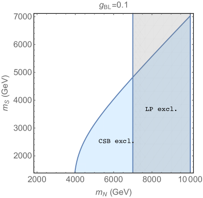
We study three different scenarios of the which is shown in Fig. 3 and to be compared to the current LHC constraints on the boson and futre GW prospects. It turns out that the vacuum stability issue is not going to be much better than in the SM, since the GW prospects of the conformal model prefer samll quartic couplings of , and a large Yukawa coupling for the RHNs would result in Landau pole problem, since they tend to dominate the running of the quartic couplings at sufficiently high scale. The Landau pole appears at a scale much lower than for both the second and third benchmark scenarios in Fig. 3; as a comparison, the first scenario is much better, benefitting from a smaller coupling . The vacuum stability and Landau pole limits on the RHN mass and the DM mass is show in Fig. 1, where we have set .
2.3 Current limits
For a TeV-scale , the mass is stringently constrained by the dilepton data (with ) at the LHC Patra:2015bga ; Lindner:2016lpp . For a sequential boson with the same couplings as in the SM, the current ATLAS and CMS 13 TeV data requires that TeV at the 95% confidence level ATLAS:2016cyf ; CMS:2016abv . The production cross section in the model can be obtained by rescaling that of a sequential heavy boson, as function of the gauge coupling Dev:2016xcp . To this end, the partial decay widths of the boson into the SM fermions, the heavy RHNs and the scalar are respectively
| (15) |
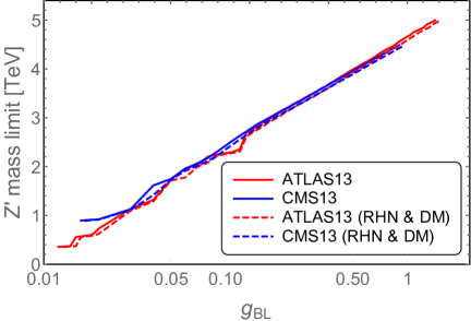
with the color factor (3 for quarks and 1 otherwise), and the baryon and lepton numbers for the SM fermions, for the quarks and charged leptons and for the light neutrinos. All these decay modes are universally proportional to the gauge coupling . In the absence of the heavy RHNs and the field, the branching fraction is a constant, being , in the limit of , and the production cross section . As a result, when gets larger, the dilepton limits on the mass tend to be stronger. The constraints from the ATLAS ATLAS:2016cyf and CMS CMS:2016abv 13 TeV data are shown respectively as the solid red and blue curves in Fig. 2. As a comparison, we also show in Fig. 2 the dilepton limits in the presence of the three RHNs and DM as the dashed curves, assuming their masses are significantly lower than thus the decays are kinematically allowed. As a result of these extra decays modes, the dilepton limits in Fig. 2 become slightly weaker. For illustration purpose, we adopt three different benchmark values of , and , interpret the solid lines in Fig. 2 and obtain the current dilepton constraints on the boson mass and the corresponding limits on , which are collected in Table 2. At the high-luminosity LHC (HL-LHC) and future 100 TeV colliders, the prospects of the boson could be largely improved Diener:2010sy ; Godfrey:2013eta ; Rizzo:2014xma .
| without RHNs & DM | with RHNs & DM | ||||
|---|---|---|---|---|---|
| [TeV] | [TeV] | [TeV] | [TeV] | ||
| 0.1 | |||||
| 0.3 | |||||
| 1.0 | |||||
3 Phase transition dynamics and gravitational wave signatures
As the Universe cools down, the EWSB is induced by the dynamical breaking of the , i.e., phase transition. If the phase transition is strong first order, GWs can be produced and potentially probed by the space-based interferometers like LISA.
3.1 Dynamical breaking and phase transition
In this section, we first demonstrate the calculation of the phase transition, which is determined by the thermal potential. The finite temperature corrections to the effective potential at one loop are given by
| (16) |
where the functions are
| (17) |
with the upper (lower) sign corresponding to bosonic (fermionic) contributions. Here, in order to describe the high- and low- behaviors appropriately, the above integrals can be expressed as a sum of the second kind of modified Bessel functions Bernon:2017jgv ,
| (18) |
The dominant contributions come from the hidden scalar , RHNs and the extra gauge field . The field dependent mass and thermal corrections are given respectively by
| (19) | |||
| (20) |
3.2 Gravitational waves signals
The bounce configuration of the nucleated bubble, i.e. the bounce configuration of the field that connects the broken vacuum (true vacuum) and the false vacuum (here it can be conserving vacuum), can be obtained by extremizing
| (21) |
through solving the equation of motion for (it is for the scenario under study),
| (22) |
with the boundary conditions of
| (23) |
At the nucleation temperature , the thermal tunneling probability for bubble nucleation per horizon volume and per horizon time is of order unity with Affleck:1980ac ; Linde:1981zj ; Linde:1980tt ,
| (24) |
Two parameters are crucial for the calculations of GW emission:
-
•
The parameter . It describes the strength of the phase transition, and is defined as the energy density released from the strong first order EWPT normalized by the total radiation energy density :
(25) where is the latent heat released in phase transition, i.e. the difference of the energy density between the false and the true vacuum.
-
•
The parameter . It describes roughly the inverse time duration of the strong first order EWPT, and characterizes the GW spectrum peak frequency, which is connected with the action through
(26) where is the Hubble parameter at the bubble nucleation temperature .
We are now ready to calculate the stochastic GW background generated during the first order phase transition. Significant progress has been made in recent years on the calculations of the GW from phase transitions (see e.g. Ref. Caprini:2015zlo ; Cai:2017cbj ; Weir:2017wfa for recent reviews). It is now generally believed that the dominant source for the GW production in this process is the sound waves (SWs) in the plasma which lasts long after the phase transition completes Hindmarsh:2013xza ; Hindmarsh:2015qta , though the bubble collision contribution has also been theoretically well modeled Jinno:2017fby ; Jinno:2017ixd ; Jinno:2016vai ; Cutting:2018tjt ; Kosowsky:1991ua ; Kosowsky:1992rz ; Kosowsky:1992vn ; Huber:2008hg . Another contribution comes from the Magnetohydrodynamic (MHD) turbulence in the magnetized plasma with high Reynolds number Caprini:2009yp ; Binetruy:2012ze . The total resultant energy density spectrum can be approximated by the following linear summation of the individual contributions above:
| (27) |
and we neglect in the following the contribution from bubble collision .
The GW spectrum from the dominant SWs can be found by fitting to the result of numerical simulations with the fluid-scalar field model Hindmarsh:2015qta :
| (28) | |||||
where is the relativistic degrees of freedom in the plasma at the time of EWPT and is the present peak frequency of the spectrum:
| (29) |
In addition, the factor is the fraction of latent heat transformed into the kinetic energy of the fluid and can be found by solving the hydrodynamic velocity profiles of the bubbles Espinosa:2010hh ; Alves:2018jsw ; Alves:2018oct .
The GW spectrum from the MHD turbulence can be theoretically modelled with inputs of the magnetic and turbulence power spectra Kosowsky:2001xp ; Caprini:2009yp ; Gogoberidze:2007an ; Niksa:2018ofa and improved by numerically evolving the MHD equations Pol:2019yex ; Brandenburg:2017neh . A fitting formula is also available Caprini:2009yp ; Binetruy:2012ze :
| (30) | |||||
Here the peak frequency is given by
| (31) |
The energy fraction tranferred to the MHD turbulence is uncertain as of now and can vary between to of Hindmarsh:2015qta . Here we take tentatively .
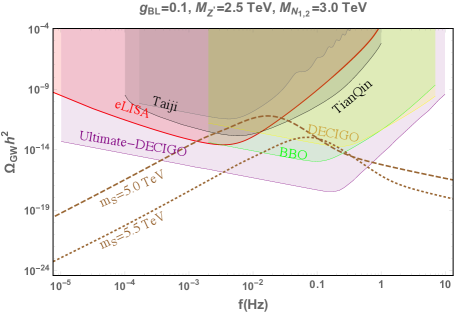
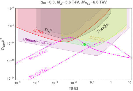
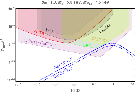
Summing up the results in Eqs. (28) and (30), we can obtain the total GW energy density spectrum. The expected GW energy spectra for three benchmark scenarios with different values are shown in Fig. 3. The color-shaded regions on the top are the experimentally sensitive regions for several proposed space-based GW detectors. As discussed earlier, the GW signal comes mainly from SWs. Our study indicates that increasing the RHN masses may leads to a decrease of the phase transition temperature, while its mass is severely bounded by the EWSB conditions given in Eq. (9). The three panels of Fig. 3 demonstrate that the amplitudes of GW signal spectra decrease as increases, which implies that the GW prospects are weaker when the charge of DM scalar is large. The hidden scalar is useful for generating the proper vacuum barrier at the nucleation temperature. Furthermore, a larger hidden scalar mass leads to a lower GW amplitude and a higher peak frequency for the GW spectrum.
To assess the discovery prospects of the GW spectra, we calculate the signal-to-noise ratio (SNR) with the definition adopted by Ref. Caprini:2015zlo :
| (32) |
where is the experimental sensitivity for the detectors and is the mission duration in unit of year for each experiment. Here we assume . For the LISA configurations with four links, the suggested threshold SNR for discovery is 50 Caprini:2015zlo . For the six link configurations as drawn here, the uncorrelated noise reduction technique can be used and the suggested SNR threshold can be as low as 10 Caprini:2015zlo . The GW spectrum of the TeV case for the and scenarios are able to be detected by LISA, with respectively and .
4 Resonant Leptogenesis
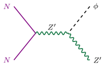
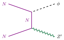
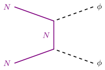
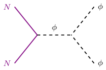
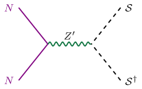
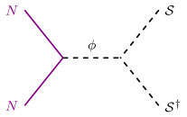
For the case of leptogenesis occurring via flavor oscillations of the heavy right-handed neutrinos in the classically conformal models, we refer the readers to Ref. Khoze:2013oga to look for some details. For TeV scale RHNs, it is necessary to use the resonant leptogenesis mechanism Covi:1996wh ; Flanz:1996fb ; Pilaftsis:1997jf ; Pilaftsis:2003gt in order to avoid the Davidson-Ibarra bound Davidson:2002qv . For simplicity, we assume the two RHN mass eigenstates and are almost degenerate with the mass and a small splitting , and the third RHN significantly heavier. The heavy boson, the conformal scalar and the DM scalar play important roles in the generation of lepton asymmetry from the decay of RHNs, as they would induce processes that dilute the heavy RHNs by two units, thus reducing the lepton and baryon asymmetry significantly in a large regions of parameter space Blanchet:2009bu ; Blanchet:2010kw ; Iso:2010mv ; Okada:2012fs ; Heeck:2016oda ; Dev:2017xry . Such processes include
| (33) |
with running over all the flavors of SM quarks, charged leptons and neutrinos. The corresponding Feynman diagrams are shown in Fig. 4. One should note that the scalar mixing between and however does not play any role in freeze-out leptogenesis since the latter takes place prior to EWSB. Thus the processes are only mediated by the gauge boson. The Feynman diagrams in (b) and (c) are mediated by the gauge and Yukawa couplings, the process in (d) and (e) by the Yukawa couplings and the scalar quartic coupling in the potential (1.4). If the DM is lighter than the RHNs , i.e. , the process in (f) and (g) is also important in some region of the parameter space, which is induced through both the gauge () and scalar () portals. There exists in principle also the process . However, in the conformal theories the RHN masses are constrained as shown in Eq. (9); with heavier than and neglecting the DM mass, Eq. (9) implies that . Then the process process is insignificant, suppressed by the kinematical space.
 |
 |
 |
| (a) | (b) | (c) |
 |
 |
 |
| (d) | (e) | (f) |
 |
||
| (g) |
The Boltzmann equations, which govern the evolution of the RHN number density and the lepton asymmetry, are given by
| (34) | |||||
| (35) |
where is a dimensionless parameter, is the Hubble expansion rate at temperature , is the number density of photons, and is the normalized number density of RHN (similarly for the lepton asymmetry). The ’s are the various thermalized interaction rates: for the RHN decay , and and the standard scattering processes as in Refs. Giudice:2003jh ; Pilaftsis:2003gt with the subscripts denoting respectively the and -channel exchange of the SM Higgs doublet or the SM gauge bosons (with ) before EWSB. Here the integration over different momenta has already been performed, assuming implicitly kinetic equilibrium. The new scattering processes in our model in Fig. 4 correspond to the scattering rates , and all the corresponding reduced cross sections are collected in Appendix B. The prefactor of 2 in Eq. (34) accounts for the reduction of RHN by unit of two Heeck:2016oda . The thermal corrections to the SM particles are included in the calculation Giudice:2003jh ; Dev:2014laa . If the term is comparable or larger than other terms on the r.h.s. of Eq. (34), these extra processes in Fig. 4 could significantly dilute the RHN number density before the sphaleron decoupling temperature GeV DOnofrio:2014rug , thus potentially making type-I seesaw freeze-out leptogenesis ineffective. Then we can set limits on the heavy particle masses and the couplings in the conformal model.
To be concrete, we consider two distinct scenarios, i.e. without and with the DM particle involved in the lepton asymmetry generation in the RHN decay, with the first one corresponding to the limit of and the second one . In both of the two cases, the dilution effect depends on the effective neutrino mass (or effectively on the Yukawa coupling ) and the CP asymmetry . Since in this paper we are mostly concerned with the role of the new particles in the lepton asymmetry generation in RHN decay , we will not consider the flavor structure details in the neutrino sector but fix , without any significant tuning or cancellation in the type-I seesaw formula for light neutrino masses Dev:2017xry . A large CP-asymmetry can then be generated by the resonant enhancement mechanism, and go up to order one if , with is the averaged RHN decay width Blanchet:2009bu ; Dev:2017wwc . For the sake of concreteness, we adopt the value of throughout this paper.
In the case without DM, the dilution effect depends also on the RHN mass , the mass , the conformal scalar mass , the quartic coupling , with the last three being functions of the gauge coupling and the scale in the conformal theory, as shown in Eqs. (8), (9) and (6). Therefore we choose the free parameters to be , and in the conformal model, with the Yukawa coupling determined by the RHN mass for fixed which enters some of the diagrams in Fig. 4. For the three benchmark values of in Table 2, the LHC dilepton limits on are shown as the horizontal dashed red, green and blue lines in the left panel of Fig. 5. As stated in Ref. Dev:2017xry , in the case without DM, if the RHN mass and , the dilution is dominated by the mediated process , benefiting from the (almost) massless fermions in the final states and the large number of degrees of freedom. One can see the clear resonance structure in the left panel of Fig. 5; this corresponds to the inverse decay process with the subsequent decay of the on-shell boson into SM fermions, which enhance largely the dilution effect. For heavy enough RHNs with and/or , the processes and/or are also important, which however is suppressed by the small Yukawa coupling when . In the left panel of Fig. 5, all the red, green and blue shaded regions are falsified by the extra diluting processes.


When the DM mass , the process would contribute to the dilution of lepton asymmetry generation, which is mediated by the and bosons, with the Feynman diagrams shown in (f) and (g) in Fig. 4. With the dashed curves in Fig. 2, the dilepton limits on the mass and the scale are slightly lower than the case without DM, as shown in Table 2. The mediated process , however, can not compete the processes , as a result of the large degrees of freedom in the SM, unless the charge of DM is very large. On the other hand, the cross section in the scalar portal is proportional to the trilinear scalar coupling , which might enhance significantly the cross section when the scale is large. Compared to the case without DM, the new scalar portal opens the possibility of new resonance, due to the resonance relation (with the RHN energy) before the RHN decays. This corresponds to the extra peak structures in the right panel of Fig. 5, where we have fixed the DM mass TeV for the sake of concreteness. As in the left panel, all the red, green and blue shaded regions are falsified by the diluting processes which reduce the RHN number by two units.
In short, all the gray and red, green and blue shaded regions in both of the two panels of Fig. 5 are falsified by the Feynman diagrams in Fig. 4; to have a viable leptogenesis framework to generate the baryon aymmetry in the early Universe, one has to choose parameters in the unshaded regions in Fig. 5. Roughly speaking, when the gauge coupling (and the quartic coupling ) gets larger, the (reduced) cross sections for the dilution processes becomes larger, and the allowed parameter space shrinks significantly, depending on the RHN mass . The bounds from the correct spontaneous symmetry breaking condition imposed by (see Eq. (9)) are also presented in both the two panels of Fig. 5, which exclude the large regions and are largely complementary to the limits from leptogenesis.
5 WIMP DM in the conformal model
In this section, we investigate the DM phenomenology in the conformal model, including the relic density of DM, direct detection and collider prospects.
5.1 Relic density and direct detection
For the GW favored benchmark scenarios, as explored in Fig. 3, DM annihilation at freezing-out is dominated by the process , and a larger charge leads to a smaller annihilation cross section, which will yield a lower value for the relic abundance of DM. The corresponding Boltzmann equation is then given by
| (36) |
with and the entropy density and Hubble parameter at the DM mass are resepctively
where is the reduced Planck mass. are respectively the equilibrium number densities of and per comoving volume. in Eq. (36) is the thermal averaged cross section and its expression is given in Appendix C. After freezing-out, the total relic abundance of DM at the present epoch is obtained through the following equation Edsjo:1997bg
| (37) |
with obtained from numerical solutions of the coupled Boltzmann equations given in Eq. (36).
Regarding the direct detection of DM, the spin-independent (SI) process is dominated by the mediated scattering of DM off the nucleon , with the cross section
| (38) |
A large here can results in a large cross section, which is excluded by LUX Akerib:2016vxi , PandaX-II Tan:2016zwf ; Cui:2017nnn and Xenon1T Aprile:2017iyp . Therefore, we do not expect the DM scalar under study will saturate all the observed DM relic abundance.
5.2 Collider signatures
The DM scalar can be produced at high-energy colliders in the scalar portal or the gauge portal. In the scalar portal, and can be pair produced through both the SM Higgs and the scalar , assisted by the mixing which is induced by the term in the potential (1). In particular, the most important production channel is from the gluon-fusion production of SM Higgs or , associated with a gluon jet emitted from the initial partons, i.e.
| (39) |
The DM particles and leaves the detectors without leaving any signal or track, and we have a high-energy jet with large missing transverse energy at colliders. However, the production cross section is suppressed by the effective loop-level couplings of and to gluons, and the LHC monojet data can not set limits on the DM sector in the model Khachatryan:2014rra ; Aad:2015zva ; Aaboud:2017phn ; Sirunyan:2017jix . In the gauge portal, the most efficient way to produce DM is from the on-shell decay in the process
| (40) |
In light of the current stringent limits on the boson mass ATLAS:2016cyf ; CMS:2016abv , as shown in Fig. 2, the monojet searches at LHC are too weak to set any limit on the DM sector Khachatryan:2014rra ; Aad:2015zva ; Aaboud:2017phn ; Sirunyan:2017jix .
6 Conclusion
In this paper we introduce a hidden scalar to the extension of the SM with classical conformal symmetry, which affects the dynamical EWSB by dimensional transmutation through the Coleman-Weinberg mechanism. The correct spontaneous symmetry breaking of the U(1)B-L symmetry restricts the scales of the hidden scalar and the RHNs. For smaller gauge coupling , a lower hidden scalar mass is crucial to realize a strong first order phase transition, and produce a GW signal to be probed by LISA. The possibility to realize the resonant leptogenesis mechanism is found to be disturbed by the hidden scalar depending on the mass hierarchy between it and the RHN. For the benchmark scenarios that can produce the LISA detectable GW signal and explain the baryon asymmetry of the Universe via resonant leptogenesis, we do not expect the dark matter relic abundance to be fully saturated by the hidden scalar introduced here.
Acknowledegments
The work of L.B. is supported by the National Natural Science Foundation of China under grant No.11605016 and No.11647307. W.C. is supported by the China Postdoctoral Science Foundation under Grant No.2019TQ0329. H.G. is partially supported by the U.S. Department of Energy grant DE-SC0009956. Y.Z. is supported by the US Department of Energy under Grant No. DE-SC0017987, and would like to thank the Center for High Energy Physics, Peking University, the Institute of Theoretical Physics, Chinese Academy of Sciences, the Tsung-Dao Lee Institute, and the Institute of High Energy Physics, Chinese Academy of Sciences for generous hospitality where the paper was partially done.
Appendix A Renormalization group equations
Following Ref. Khoze:2014xha , the RGEs for the scalar quartic couplings in the conformal model read
| (41) |
with
| (42) | |||||
| (43) | |||||
| (44) | |||||
| (45) | |||||
| (46) | |||||
| (47) |
where with the gauge coupling for the SM gauge groups and , is the SM top Yukawa coupling. For simplicity we have neglected all other Yukawa couplings in the SM as well as the couplings which are much smaller. For the top quark Yukawa coupling and the coupling for the three RHNs, the RGEs are respectively
| (48) | |||||
| (49) |
and the RGEs for the gauge couplings are given by
| (50) |
where the gauge coupling for the SM gauge group .
Appendix B Reduced cross sections for leptogenesis
In this appendix, we list the explicit analytic formulas for the reduced cross sections for various scatterings involving the RHNs used in our leptogenesis calculations in Sec. 4. All the relevant Feynman diagrams can be found in Fig. 4. For the fermionic channels,
| (51) |
with , , and the symmetry factor for the charged fermions and for neutrinos. For the bosonic channels,
| (52) | |||||
| (53) |
with the and terms
| (54) | |||||
| (55) | |||||
| (56) | |||||
| (57) | |||||
| (58) | |||||
| (59) | |||||
where and
| (60) | |||||
| (61) |
At the resonance, i.e. , the propagator should be modified accordingly to include the width. For the DM channel,
| (62) | |||||
with , and
| (63) |
Appendix C DM annihilation cross section
Once the kinematical threshold is open, the dominant contribution to the DM pairs annihilations channel is , with the corresponding momenta of incoming and outgoing particles. The squared amplitude is calculated using CalCHEP Belyaev:2012qa with model files prepared by FeynRules Alloul:2013bka ,
| (64) | |||||
with
| (65) | |||||
| (66) |
Here, the for small mixing between the SM Higgs and the Higgs . With the squared amplitude at hand, the cross section is given by
| (67) |
The thermal averaged annihilation cross section are obtained in terms of annihilation cross section and the second kind modified Bessel function Gondolo:1990dk
| (68) |
References
- (1) S. R. Coleman and E. J. Weinberg, “Radiative Corrections as the Origin of Spontaneous Symmetry Breaking,” Phys. Rev. D7 (1973) 1888–1910.
- (2) C. Englert, J. Jaeckel, V. V. Khoze, and M. Spannowsky, “Emergence of the Electroweak Scale through the Higgs Portal,” JHEP 04 (2013) 060, arXiv:1301.4224 [hep-ph].
- (3) A. Farzinnia, H.-J. He, and J. Ren, “Natural Electroweak Symmetry Breaking from Scale Invariant Higgs Mechanism,” Phys. Lett. B727 (2013) 141–150, arXiv:1308.0295 [hep-ph].
- (4) V. V. Khoze, “Inflation and Dark Matter in the Higgs Portal of Classically Scale Invariant Standard Model,” JHEP 11 (2013) 215, arXiv:1308.6338 [hep-ph].
- (5) S. Iso, N. Okada, and Y. Orikasa, “Classically conformal L extended Standard Model,” Phys. Lett. B676 (2009) 81–87, arXiv:0902.4050 [hep-ph].
- (6) LISA Collaboration, H. Audley et al., “Laser Interferometer Space Antenna,” arXiv:1702.00786 [astro-ph.IM].
- (7) T. Robson, N. J. Cornish, and C. Liug, “The construction and use of LISA sensitivity curves,” Class. Quant. Grav. 36 no. 10, (2019) 105011, arXiv:1803.01944 [astro-ph.HE].
- (8) X. Gong et al., “Descope of the ALIA mission,” J. Phys. Conf. Ser. 610 no. 1, (2015) 012011, arXiv:1410.7296 [gr-qc].
- (9) TianQin Collaboration, J. Luo et al., “TianQin: a space-borne gravitational wave detector,” Class. Quant. Grav. 33 no. 3, (2016) 035010, arXiv:1512.02076 [astro-ph.IM].
- (10) V. Corbin and N. J. Cornish, “Detecting the cosmic gravitational wave background with the big bang observer,” Class. Quant. Grav. 23 (2006) 2435–2446, arXiv:gr-qc/0512039 [gr-qc].
- (11) DECIGO Working group Collaboration, M. Musha, “Space gravitational wave detector DECIGO/pre-DECIGO,” Proc. SPIE Int. Soc. Opt. Eng. 10562 (2017) 105623T.
- (12) H. Kudoh, A. Taruya, T. Hiramatsu, and Y. Himemoto, “Detecting a gravitational-wave background with next-generation space interferometers,” Phys. Rev. D73 (2006) 064006, arXiv:gr-qc/0511145 [gr-qc].
- (13) J. Ellis, M. Lewicki, J. M. No, and V. Vaskonen, “Gravitational wave energy budget in strongly supercooled phase transitions,” JCAP 1906 no. 06, (2019) 024, arXiv:1903.09642 [hep-ph].
- (14) J. Ellis, M. Lewicki, and J. M. No, “On the Maximal Strength of a First-Order Electroweak Phase Transition and its Gravitational Wave Signal,” arXiv:1809.08242 [hep-ph]. [JCAP1904,003(2019)].
- (15) R. Jinno and M. Takimoto, “Probing a classically conformal B-L model with gravitational waves,” Phys. Rev. D95 no. 1, (2017) 015020, arXiv:1604.05035 [hep-ph].
- (16) S. Iso, P. D. Serpico, and K. Shimada, “QCD-Electroweak First-Order Phase Transition in a Supercooled Universe,” Phys. Rev. Lett. 119 no. 14, (2017) 141301, arXiv:1704.04955 [hep-ph].
- (17) W. Chao, H.-K. Guo, and J. Shu, “Gravitational Wave Signals of Electroweak Phase Transition Triggered by Dark Matter,” JCAP 1709 no. 09, (2017) 009, arXiv:1702.02698 [hep-ph].
- (18) W. Chao, W.-F. Cui, H.-K. Guo, and J. Shu, “Gravitational Wave Imprint of New Symmetry Breaking,” arXiv:1707.09759 [hep-ph].
- (19) P. Minkowski, “ at a Rate of One Out of Muon Decays?,” Phys. Lett. 67B (1977) 421–428.
- (20) R. N. Mohapatra and G. Senjanovic, “Neutrino Mass and Spontaneous Parity Nonconservation,” Phys. Rev. Lett. 44 (1980) 912. [,231(1979)].
- (21) T. Yanagida, “Horizontal gauge symmetry and masses of neutrinos,” Conf. Proc. C7902131 (1979) 95–99.
- (22) M. Gell-Mann, P. Ramond, and R. Slansky, “Complex Spinors and Unified Theories,” Conf. Proc. C790927 (1979) 315–321, arXiv:1306.4669 [hep-th].
- (23) S. L. Glashow, “The Future of Elementary Particle Physics,” NATO Sci. Ser. B 61 (1980) 687.
- (24) M. Fukugita and T. Yanagida, Phys. Lett. B 174, 45 (1986).
- (25) V. V. Khoze and G. Ro, “Leptogenesis and Neutrino Oscillations in the Classically Conformal Standard Model with the Higgs Portal,” JHEP 10 (2013) 075, arXiv:1307.3764 [hep-ph].
- (26) L. Covi, E. Roulet, and F. Vissani, “CP violating decays in leptogenesis scenarios,” Phys. Lett. B384 (1996) 169–174, arXiv:hep-ph/9605319 [hep-ph].
- (27) M. Flanz, E. A. Paschos, U. Sarkar, and J. Weiss, “Baryogenesis through mixing of heavy Majorana neutrinos,” Phys. Lett. B389 (1996) 693–699, arXiv:hep-ph/9607310 [hep-ph].
- (28) A. Pilaftsis, “CP violation and baryogenesis due to heavy Majorana neutrinos,” Phys. Rev. D56 (1997) 5431–5451, arXiv:hep-ph/9707235 [hep-ph].
- (29) A. Pilaftsis and T. E. J. Underwood, “Resonant leptogenesis,” Nucl. Phys. B692 (2004) 303–345, arXiv:hep-ph/0309342 [hep-ph].
- (30) S. Blanchet, Z. Chacko, S. S. Granor, and R. N. Mohapatra, “Probing Resonant Leptogenesis at the LHC,” Phys. Rev. D82 (2010) 076008, arXiv:0904.2174 [hep-ph].
- (31) S. Blanchet, P. S. B. Dev, and R. N. Mohapatra, “Leptogenesis with TeV Scale Inverse Seesaw in SO(10),” Phys. Rev. D82 (2010) 115025, arXiv:1010.1471 [hep-ph].
- (32) S. Iso, N. Okada, and Y. Orikasa, “Resonant Leptogenesis in the Minimal B-L Extended Standard Model at TeV,” Phys. Rev. D83 (2011) 093011, arXiv:1011.4769 [hep-ph].
- (33) N. Okada, Y. Orikasa, and T. Yamada, “Minimal Flavor Violation in the Minimal Model and Resonant Leptogenesis,” Phys. Rev. D86 (2012) 076003, arXiv:1207.1510 [hep-ph].
- (34) J. Heeck and D. Teresi, “Leptogenesis and neutral gauge bosons,” Phys. Rev. D94 no. 9, (2016) 095024, arXiv:1609.03594 [hep-ph].
- (35) P. S. B. Dev, R. N. Mohapatra, and Y. Zhang, “Leptogenesis constraints on breaking Higgs boson in TeV scale seesaw models,” JHEP 03 (2018) 122, arXiv:1711.07634 [hep-ph].
- (36) T. Hambye, A. Strumia, and D. Teresi, “Super-cool Dark Matter,” JHEP 08 (2018) 188, arXiv:1805.01473 [hep-ph].
- (37) W. Rodejohann and C. E. Yaguna, “Scalar dark matter in the B-L model,” JCAP 1512 no. 12, (2015) 032, arXiv:1509.04036 [hep-ph].
- (38) CMS Collaboration, V. Khachatryan et al., “Search for dark matter, extra dimensions, and unparticles in monojet events in proton Cproton collisions at TeV,” Eur. Phys. J. C75 no. 5, (2015) 235, arXiv:1408.3583 [hep-ex].
- (39) ATLAS Collaboration, G. Aad et al., “Search for new phenomena in final states with an energetic jet and large missing transverse momentum in pp collisions at 8 TeV with the ATLAS detector,” Eur. Phys. J. C75 no. 7, (2015) 299, arXiv:1502.01518 [hep-ex]. [Erratum: Eur. Phys. J.C75,no.9,408(2015)].
- (40) ATLAS Collaboration, M. Aaboud et al., “Search for dark matter and other new phenomena in events with an energetic jet and large missing transverse momentum using the ATLAS detector,” JHEP 01 (2018) 126, arXiv:1711.03301 [hep-ex].
- (41) CMS Collaboration, A. M. Sirunyan et al., “Search for new physics in final states with an energetic jet or a hadronically decaying or boson and transverse momentum imbalance at ,” Phys. Rev. D97 no. 9, (2018) 092005, arXiv:1712.02345 [hep-ex].
- (42) LUX Collaboration, D. S. Akerib et al., “Results from a search for dark matter in the complete LUX exposure,” Phys. Rev. Lett. 118 no. 2, (2017) 021303, arXiv:1608.07648 [astro-ph.CO].
- (43) PandaX-II Collaboration, A. Tan et al., “Dark Matter Results from First 98.7 Days of Data from the PandaX-II Experiment,” Phys. Rev. Lett. 117 no. 12, (2016) 121303, arXiv:1607.07400 [hep-ex].
- (44) PandaX-II Collaboration, X. Cui et al., “Dark Matter Results From 54-Ton-Day Exposure of PandaX-II Experiment,” Phys. Rev. Lett. 119 no. 18, (2017) 181302, arXiv:1708.06917 [astro-ph.CO].
- (45) XENON Collaboration, E. Aprile et al., “First Dark Matter Search Results from the XENON1T Experiment,” Phys. Rev. Lett. 119 no. 18, (2017) 181301, arXiv:1705.06655 [astro-ph.CO].
- (46) A. Biswas, S. Choubey and S. Khan, JHEP 1608, 114 (2016) [arXiv:1604.06566 [hep-ph]].
- (47) S. Patra, F. S. Queiroz, and W. Rodejohann, “Stringent Dilepton Bounds on Left-Right Models using LHC data,” Phys. Lett. B752 (2016) 186–190, arXiv:1506.03456 [hep-ph].
- (48) M. Lindner, F. S. Queiroz, and W. Rodejohann, “Dilepton bounds on left Cright symmetry at the LHC run II and neutrinoless double beta decay,” Phys. Lett. B762 (2016) 190–195, arXiv:1604.07419 [hep-ph].
- (49) ATLAS Collaboration, T. A. collaboration, “Search for new high-mass resonances in the dilepton final state using proton-proton collisions at = 13 TeV with the ATLAS detector,”.
- (50) CMS Collaboration, C. Collaboration, “Search for a high-mass resonance decaying into a dilepton final state in 13 fb-1 of pp collisions at ,”.
- (51) P. S. Bhupal Dev, R. N. Mohapatra, and Y. Zhang, “Naturally stable right-handed neutrino dark matter,” JHEP 11 (2016) 077, arXiv:1608.06266 [hep-ph].
- (52) R. Diener, S. Godfrey, and T. A. W. Martin, “Unravelling an Extra Neutral Gauge Boson at the LHC using Third Generation Fermions,” Phys. Rev. D83 (2011) 115008, arXiv:1006.2845 [hep-ph].
- (53) S. Godfrey and T. Martin, “Z’ Discovery Reach at Future Hadron Colliders: A Snowmass White Paper,” in Proceedings, 2013 Community Summer Study on the Future of U.S. Particle Physics: Snowmass on the Mississippi (CSS2013): Minneapolis, MN, USA, July 29-August 6, 2013. 2013. arXiv:1309.1688 [hep-ph]. http://www.slac.stanford.edu/econf/C1307292/docs/submittedArxivFiles/1309.1688.pdf.
- (54) T. G. Rizzo, “Exploring new gauge bosons at a 100 TeV collider,” Phys. Rev. D89 no. 9, (2014) 095022, arXiv:1403.5465 [hep-ph].
- (55) J. Bernon, L. Bian, and Y. Jiang, “A new insight into the phase transition in the early Universe with two Higgs doublets,” JHEP 05 (2018) 151, arXiv:1712.08430 [hep-ph].
- (56) I. Affleck, “Quantum Statistical Metastability,” Phys. Rev. Lett. 46 (1981) 388.
- (57) A. D. Linde, “Decay of the False Vacuum at Finite Temperature,” Nucl. Phys. B216 (1983) 421. [Erratum: Nucl. Phys.B223,544(1983)].
- (58) A. D. Linde, “Fate of the False Vacuum at Finite Temperature: Theory and Applications,” Phys. Lett. 100B (1981) 37–40.
- (59) C. Caprini et al., “Science with the space-based interferometer eLISA. II: Gravitational waves from cosmological phase transitions,” JCAP 1604 no. 04, (2016) 001, arXiv:1512.06239 [astro-ph.CO].
- (60) R.-G. Cai, Z. Cao, Z.-K. Guo, S.-J. Wang, and T. Yang, “The Gravitational-Wave Physics,” Natl. Sci. Rev. 4 no. 5, (2017) 687–706, arXiv:1703.00187 [gr-qc].
- (61) D. J. Weir, “Gravitational waves from a first order electroweak phase transition: a brief review,” Phil. Trans. Roy. Soc. Lond. A376 no. 2114, (2018) 20170126, arXiv:1705.01783 [hep-ph].
- (62) M. Hindmarsh, S. J. Huber, K. Rummukainen, and D. J. Weir, “Gravitational waves from the sound of a first order phase transition,” Phys. Rev. Lett. 112 (2014) 041301, arXiv:1304.2433 [hep-ph].
- (63) M. Hindmarsh, S. J. Huber, K. Rummukainen, and D. J. Weir, “Numerical simulations of acoustically generated gravitational waves at a first order phase transition,” Phys. Rev. D92 no. 12, (2015) 123009, arXiv:1504.03291 [astro-ph.CO].
- (64) R. Jinno and M. Takimoto, “Gravitational waves from bubble dynamics: Beyond the Envelope,” JCAP 1901 (2019) 060, arXiv:1707.03111 [hep-ph].
- (65) R. Jinno, S. Lee, H. Seong, and M. Takimoto, “Gravitational waves from first-order phase transitions: Towards model separation by bubble nucleation rate,” JCAP 1711 (2017) 050, arXiv:1708.01253 [hep-ph].
- (66) R. Jinno and M. Takimoto, “Gravitational waves from bubble collisions: An analytic derivation,” Phys. Rev. D95 no. 2, (2017) 024009, arXiv:1605.01403 [astro-ph.CO].
- (67) D. Cutting, M. Hindmarsh, and D. J. Weir, “Gravitational waves from vacuum first-order phase transitions: from the envelope to the lattice,” Phys. Rev. D97 no. 12, (2018) 123513, arXiv:1802.05712 [astro-ph.CO].
- (68) A. Kosowsky, M. S. Turner, and R. Watkins, “Gravitational radiation from colliding vacuum bubbles,” Phys. Rev. D45 (1992) 4514–4535.
- (69) A. Kosowsky, M. S. Turner, and R. Watkins, “Gravitational waves from first order cosmological phase transitions,” Phys. Rev. Lett. 69 (1992) 2026–2029.
- (70) A. Kosowsky and M. S. Turner, “Gravitational radiation from colliding vacuum bubbles: envelope approximation to many bubble collisions,” Phys. Rev. D47 (1993) 4372–4391, arXiv:astro-ph/9211004 [astro-ph].
- (71) S. J. Huber and T. Konstandin, “Gravitational Wave Production by Collisions: More Bubbles,” JCAP 0809 (2008) 022, arXiv:0806.1828 [hep-ph].
- (72) C. Caprini, R. Durrer, and G. Servant, “The stochastic gravitational wave background from turbulence and magnetic fields generated by a first-order phase transition,” JCAP 0912 (2009) 024, arXiv:0909.0622 [astro-ph.CO].
- (73) P. Binetruy, A. Bohe, C. Caprini, and J.-F. Dufaux, “Cosmological Backgrounds of Gravitational Waves and eLISA/NGO: Phase Transitions, Cosmic Strings and Other Sources,” JCAP 1206 (2012) 027, arXiv:1201.0983 [gr-qc].
- (74) J. R. Espinosa, T. Konstandin, J. M. No, and G. Servant, “Energy Budget of Cosmological First-order Phase Transitions,” JCAP 1006 (2010) 028, arXiv:1004.4187 [hep-ph].
- (75) A. Alves, T. Ghosh, H.-K. Guo, K. Sinha, and D. Vagie, “Collider and Gravitational Wave Complementarity in Exploring the Singlet Extension of the Standard Model,” JHEP 04 (2019) 052, arXiv:1812.09333 [hep-ph].
- (76) A. Alves, T. Ghosh, H.-K. Guo, and K. Sinha, “Resonant Di-Higgs Production at Gravitational Wave Benchmarks: A Collider Study using Machine Learning,” JHEP 12 (2018) 070, arXiv:1808.08974 [hep-ph].
- (77) A. Kosowsky, A. Mack, and T. Kahniashvili, “Gravitational radiation from cosmological turbulence,” Phys. Rev. D66 (2002) 024030, arXiv:astro-ph/0111483 [astro-ph].
- (78) G. Gogoberidze, T. Kahniashvili, and A. Kosowsky, “The Spectrum of Gravitational Radiation from Primordial Turbulence,” Phys. Rev. D76 (2007) 083002, arXiv:0705.1733 [astro-ph].
- (79) P. Niksa, M. Schlederer, and G. Sigl, “Gravitational Waves produced by Compressible MHD Turbulence from Cosmological Phase Transitions,” Class. Quant. Grav. 35 no. 14, (2018) 144001, arXiv:1803.02271 [astro-ph.CO].
- (80) A. R. Pol, S. Mandal, A. Brandenburg, T. Kahniashvili, and A. Kosowsky, “Numerical Simulations of Gravitational Waves from Early-Universe Turbulence,” arXiv:1903.08585 [astro-ph.CO].
- (81) A. Brandenburg, T. Kahniashvili, S. Mandal, A. R. Pol, A. G. Tevzadze, and T. Vachaspati, “Evolution of hydromagnetic turbulence from the electroweak phase transition,” Phys. Rev. D96 no. 12, (2017) 123528, arXiv:1711.03804 [astro-ph.CO].
- (82) S. Davidson and A. Ibarra, “A Lower bound on the right-handed neutrino mass from leptogenesis,” Phys. Lett. B535 (2002) 25–32, arXiv:hep-ph/0202239 [hep-ph].
- (83) G. F. Giudice, A. Notari, M. Raidal, A. Riotto, and A. Strumia, “Towards a complete theory of thermal leptogenesis in the SM and MSSM,” Nucl. Phys. B685 (2004) 89–149, arXiv:hep-ph/0310123 [hep-ph].
- (84) P. S. Bhupal Dev, P. Millington, A. Pilaftsis, and D. Teresi, “Flavour Covariant Transport Equations: an Application to Resonant Leptogenesis,” Nucl. Phys. B886 (2014) 569–664, arXiv:1404.1003 [hep-ph].
- (85) M. D’Onofrio, K. Rummukainen, and A. Tranberg, “Sphaleron Rate in the Minimal Standard Model,” Phys. Rev. Lett. 113 no. 14, (2014) 141602, arXiv:1404.3565 [hep-ph].
- (86) B. Dev, M. Garny, J. Klaric, P. Millington, and D. Teresi, “Resonant enhancement in leptogenesis,” Int. J. Mod. Phys. A33 (2018) 1842003, arXiv:1711.02863 [hep-ph].
- (87) J. Edsjo and P. Gondolo, “Neutralino relic density including coannihilations,” Phys. Rev. D56 (1997) 1879–1894, arXiv:hep-ph/9704361 [hep-ph].
- (88) V. V. Khoze, C. McCabe and G. Ro, JHEP 1408, 026 (2014) [arXiv:1403.4953 [hep-ph]].
- (89) A. Belyaev, N. D. Christensen and A. Pukhov, Comput. Phys. Commun. 184, 1729 (2013) doi:10.1016/j.cpc.2013.01.014 [arXiv:1207.6082 [hep-ph]].
- (90) A. Alloul, N. D. Christensen, C. Degrande, C. Duhr and B. Fuks, Comput. Phys. Commun. 185, 2250 (2014) doi:10.1016/j.cpc.2014.04.012 [arXiv:1310.1921 [hep-ph]].
- (91) P. Gondolo and G. Gelmini, “Cosmic abundances of stable particles: Improved analysis,” Nucl. Phys. B360 (1991) 145–179.