Hug and Hop: a discrete-time, non-reversible Markov chain Monte Carlo algorithm

Abstract

We introduced the Hug and Hop Markov chain Monte Carlo algorithm for estimating expectations with respect to an intractable distribution. The algorithm alternates between two kernels: Hug and Hop. Hug is a non-reversible kernel that repeatedly applies the bounce mechanism from the recently proposed Bouncy Particle Sampler to produce a proposal point far from the current position, yet on almost the same contour of the target density, leading to a high acceptance probability. Hug is complemented by Hop, which deliberately proposes jumps between contours and has an efficiency that degrades very slowly with increasing dimension. There are many parallels between Hug and Hamiltonian Monte Carlo using a leapfrog integrator, including the order of the integration scheme, however Hug is also able to make use of local Hessian information without requiring implicit numerical integration steps, and its performance is not terminally affected by unbounded gradients of the log-posterior. We test Hug and Hop empirically on a variety of toy targets and real statistical models and find that it can, and often does, outperform Hamiltonian Monte Carlo.

Keywords: MCMC; bouncy particle samplers; gradient-based proposals; scaling limit.

1 Introduction

Markov chain Monte Carlo (MCMC) algorithms approximate expectations under an un-normalised target distribution of $\pi$ by simulating a Markov chain with $\pi$ as its stationary distribution then computing empirical averages over the simulated values of the chain. Historically MCMC has been based on reversible Markov kernels such as the Metropolis-Hastings kernel Hastings, (1970) and special cases and variations of this (e.g. Brooks et al.,, 2011) since it is straightforward to ensure that these target $\pi$. However, there has been much recent interest in non-reversible kernels (e.g. Bouchard-Côté et al.,, 2018; Fearnhead et al.,, 2018) which have the potential both in practice and in theory to be more efficient than their reversible counterparts (Neal,, 1998; Diaconis et al.,, 2000; Bierkens,, 2015; Ma et al.,, 2018). A particular continuous-time non-reversible algorithm, the Bouncy Particle Sampler (Peters and de With,, 2012; Bouchard-Côté et al.,, 2018) and variations such as the coordinate sampler (Wu and Robert,, 2020) and the Discrete Bouncy Particle Sampler (Bouchard-Côté et al.,, 2018; Sherlock and Thiery,, 2021) and variations on both bouncy samplers (Vanetti et al.,, 2017), use occasional reflections of a velocity in the hyperplane perpendicular to the current gradient to eliminate (for continuous-time versions) or substantially reduce (discrete-time versions) rejections of proposed moves.

We introduce a novel, discrete-time, non-reversible sampling algorithm which itself consists of two accept-reject MCMC kernels, applied in alternation. Given a current value, the first kernel uses the bounce mechanism of the bouncy particle samplers to evolve a skew-reversible approximation to a flow with constant speed along a level set of $\pi$ so as to produce a proposal point that is far from the current position, yet on almost the same posterior contour, leading to a high acceptance probability; we denote this contour-hugging kernel Hug.

The second kernel complements the first by focusing on moving between contours. It encourages the next state of the Markov chain to lie on a substantially different contour by proposing a new point from a distribution centered on the current point, with a high variance in the gradient direction, and a lower variance in directions perpendicular to the gradient; we denote this kernel Hop, and the combination of the two Hug and Hop. Pseudo-code for the full algorithm is given in Appendix A.

1.1 Notation

Throughout the article the target is assumed to have a density of $\pi$ with respect to Lebesgue measure. The log-density is denoted by $\ell(x)=\log\pi(x)$ and its gradient and Hessian are denoted by $g(x)=\nabla\ell(x)$ and $H(x)=[\partial^{2}\ell/\partial x_{i}\partial x_{j}]$, while the unit gradient vector is denoted by $\widehat{g}(x)=g(x)/\left|\left|{g(x)}\right|\right|$. For some small $\epsilon>0$, when the negative Hessian is positive definite with all eigenvalues above $\epsilon$, we write $\Sigma(x)=-H(x)^{-1}$. Otherwise, we set $\Sigma(x)=-L^{\top}\{1/(\left|{\Lambda}\right|+\epsilon I_{d})\}L$, where $L^{\top}\Lambda L$ is the spectral decomposition of $H$ and $|\Lambda|$ denotes the (diagonal) matrix whose elements are the absolute values of the corresponding elements of $\Lambda$. $\Sigma(x)$ can therefore be considered as a local variance-covariance matrix with eigenvalues informed by the local curvature along each principal component, whether this curvature is positive or negative. Given $\Sigma(x)$, the matrix $A(x)$ always denotes a $d\times d$ matrix square-root of $\Sigma(x)$; i.e., $A(x)^{\top}A(x)=\Sigma(x)$.

For a matrix $M$, we use the shorthand $M^{-\top}=\left(M^{-1}\right)^{\top}$ and we refer to its induced $\ell^{2}$ norm as: $\left|\left|{M}\right|\right|_{I}=\sup_{x\in\mathbb{R}^{d}\setminus\{0\}}\left|\left|{Mx}\right|\right|_{2}/\left|\left|{x}\right|\right|_{2}$.

2 The Hug and Hop kernels

2.1 The Hug kernel

Given a current velocity, $v$ and a gradient vector, $g$, at the current position, the Bouncy Particle Sampler reflects the velocity in the hyper-plane tangent to the gradient as follows:

$$~{}\mathsf{R}\left({v;g}\right)=v-2(v^{\top}\widehat{g})\widehat{g}.$$ (1)

A single application of the Hug kernel repeatedly alternates straight-line movement using the current velocity with an application of this reflection move to repeatedly ‘bounce’ the current velocity off the hyperplane tangent to the local gradient and hence keep the net movement in the gradient direction small. The proposal mechanism from a current sample point $x=x_{0}$ samples an initial velocity, $v_{0}$, from a proposal distribution $q$ which satisfies $q(v\mid x)=q(-v\mid x)$ but does not force initial velocity to be perpendicular to the current gradient. Given a time interval, $T$, and a number of bounces, $B$, both tuning parameters, the discretisation interval is set to $\delta=T/B$, and the Hug kernel repeats the following $B$ times: firstly move to $x_{b}^{\prime}:=x_{b}+\delta v_{b}/2$, then reflect the velocity in the gradient at $x_{b}^{\prime}$: $v_{b+1}=\mathsf{R}\left({v_{b};g(x_{b}^{\prime})}\right)$, and finally move to $x_{b+1}=x_{b}^{\prime}+\delta v_{b+1}/2$. The steps below describe a single application of the kernel, $\mathsf{P_{hug}}$.

• Require: integration time, $T$; # steps, $B$; current value, $x$; symmetric proposal density $q(\cdot|x)$.

• $x_{0}\longleftarrow x$ and $\delta\longleftarrow T/B$.

• Draw velocity $v_{0}\sim q(\cdot|x_{0})$ .

• For $b=0,\ldots,B-1$

  1. Move to $x_{b}^{\prime}=x_{b}+\delta v_{b}/2$.

  2. Reflect: $v_{b+1}\longleftarrow~{}\mathsf{R}\left({v_{b};g(x_{b}^{\prime})}\right)$.

  3. Move to $x_{b+1}=x_{b}^{\prime}+\delta v_{b+1}/2$.

• Compute $\log r_{hug}=\ell(x_{B})-\ell(x_{0})+\log q(v_{B}|x_{B})-\log q(v_{0}|x_{0})$.

• With a probability of $\alpha_{hug}=1\wedge r_{hug}$, $x\longleftarrow x_{B}$; else $x\longleftarrow x$.

$\mathsf{P_{hug}}$, can be viewed as the composition of two reversible kernels each of which preserves detailed balance with respect to the extended target of $\widetilde{\pi}(x,v):=\pi(x)q(v\mid x)$. Let $\mathsf{P_{hugR}}$ be exactly as $\mathsf{P_{hug}}$, except that the proposed velocity is $-v_{B}$ rather than $v_{B}$, and let $\mathsf{P_{flip}}:(x,v)\rightarrow(x,-v)$, so that $\mathsf{P_{hug}}=\mathsf{P_{flip}}\mathsf{P_{hugR}}$. Since $q$ is symmetric, $\mathsf{P_{flip}}$ preserves $\widetilde{\pi}$. To see that $\mathsf{P_{hugR}}$ preserves $\widetilde{\pi}$, and hence so does $\mathsf{P_{hug}}$, we first consider the loop within $\mathsf{P_{hugR}}$. The transformation involves a reflection of velocity, sandwiched between two translations of position; each of these individual transformations has a Jacobian of $1$ and so the Jacobian for the entire transformation from $(x_{0},v_{0})$ to $(x_{B},-v_{B})$ is also $1$. Hence, if $X$ is stationary, the joint density of $(x_{B},-v_{B})$ is equal to $\pi(x_{0})q(v_{0}\mid x_{0})$. Secondly, the loop is skew symmetric, so that starting from $(x_{B},-v_{B})$ and iterating the loop $B$ times, then flipping the velocity would lead back to $(x_{0},v_{0})$, so, at stationarity, the joint density for the reverse move is $\pi(x_{B})q(-v_{B}\mid x_{B})=\pi(x_{B})q(v_{B}\mid x_{B})$. Hence the acceptance probability $\alpha$ in the Hug Algorithm leads to $\mathsf{P_{hugR}}$ being reversible with respect to $\pi(x)q(v\mid x)$.

2.2 Error analysis for Hug

To show why the hug kernel is effective as an MCMC proposal mechanism, consider the step from $x_{b}$ to $x_{b+1}$. Taylor expanding about the bounce point $x_{b}^{\prime}$, and noting that $x_{b}^{\prime}-x_{b}=\frac{\delta}{2}v_{b}$ and $x_{b+1}-x_{b}^{\prime}=\frac{\delta}{2}v_{b+1}$ gives:

$$\ell(x_{b}) =\ell(x_{b}^{\prime})-\frac{\delta}{2}v_{b}^{\top}g(x_{b}^{\prime})+\frac{\delta^{2}}{8}v_{b}^{\top}H(x_{b}^{+})v_{b},$$

$$\ell(x_{b+1}) =\ell(x_{b}^{\prime})+\frac{\delta}{2}v_{b+1}^{\top}g(x_{b}^{\prime})+\frac{\delta^{2}}{8}v_{b+1}^{\top}H(x_{b+1}^{-})v_{b+1},$$

where $x_{b}^{+}$ lies on the line between $x_{b}$ and $x_{b}^{\prime}$, and $x_{b+1}^{-}$ lies on the line between $x_{b}^{\prime}$ and $x_{b+1}$. Now $(v_{b}+v_{b+1})^{\top}g(x_{b}^{\prime})=2v_{b}^{\top}g(x_{b}^{\prime})-2(v_{b}^{\top}\widehat{g}(x_{b}^{\prime}))\left|\left|{g(x_{b}^{\prime})}\right|\right|=0$, so:

$$\ell(x_{b+1})-\ell(x_{b})=\frac{\delta^{2}}{8}\left[v_{b+1}^{\top}H(x_{b+1}^{-})v_{b+1}-v_{b}^{\top}H(x_{b}^{+})v_{b}\right].$$ (2)

Integrating for a time $T=B\delta$ requires $T/\delta$ such steps and might be supposed to lead to an error of $\mathcal{O}\left(\delta\right)$. However, due to the special structure of the path, if the Hessian is well behaved the full integration also has an error of $\mathcal{O}\left(\delta^{2}\right)$. We require the following conditions to obtain the theorem that follows, which is proved in Appendix B.1.

Condition 1 (Lipshitz-continuous Hessian).

There exists some $\gamma>0$, such that $\left|\left|{H(y)-H(x)}\right|\right|_{I}\leq\gamma\left|\left|{y-x}\right|\right|$ for all $x,y\in\mathbb{R}^{d}$.

Condition 2 (Bounded Hessian).

There exists some $\beta>0$, such that $\sup_{x\in\mathbb{R}^{d}}\left|\left|{H(x)}\right|\right|_{I}\leq\beta<\infty$.

Theorem 1.

Consider a target $\pi$ such that the Hessian $H(x)$ of $\ell(x)=\log\pi(x)$ satisfies Conditions 1 and  2. For a single iteration of Hug with initial velocity $v_{0}$,

$$|\ell(x_{B})-\ell(x_{0})|\leq\frac{1}{8}\delta^{2}\left|\left|{v_{0}}\right|\right|^{2}(2\beta+\gamma D),$$

where $D=\left|\left|{v_{0}T}\right|\right|$ is the total distance travelled in time $T$.

The larger $\beta$ and/or $\gamma$, the smaller $\delta$ must be. Potential consequences when Conditions 1 and/or 2 are not satisfied are illustrated in Appendix C.2. In practice, the size of $\delta$ that can be safely chosen is limited by the most extreme curvature on any surface of constant $\pi$ along which which large moves will be needed.

The only velocity changes are reflections, so $\left|\left|{v_{B}}\right|\right|=\left|\left|{v_{0}}\right|\right|$. Thus if $q$ is isotropic and independent of $x$, rather than simply symmetric, then $\alpha=1\wedge\exp[\ell(x_{B})-\ell(x_{0})]=\mathcal{O}\left(\delta^{2}\right)$. In practice, for the standard version of $\mathsf{P_{hug}}$ we choose a $q$ that is independent of $x$, and potential global anisotropy can be dealt with by pre-conditioning, as we now discuss.

2.3 Preconditioning of Hug

Typically, preconditioning according to the overall shape of the target can lead to large improvements in efficiency (e.g. Roberts and Rosenthal,, 2001; Sherlock et al.,, 2010). As in many other algorithms, such as the random-walk Metropolis (Hastings,, 1970) or Metropolis-adjusted Langevin algorithm (Besag,, 1994; Roberts and Rosenthal,, 1998), the shape of the proposal distribution should aim to mimic the shape of the target and it might be preferable to employ an elliptically symmetric proposal such as $V_{b}\mid x_{b}\sim\mathsf{N}(x_{b},\Sigma)$, where $\Sigma$ is some approximation to the variance matrix of $X$ under $\pi$. The target $\tilde{x}=A^{-\top}x$, where $A^{\top}A=\Sigma$, has $\mbox{Var}[\widetilde{X}]=I$, and a natural, isotropic proposal on this target is equivalent to the elliptical proposal on the original target. However, the bounce kernel also has a reflection move, and the standard bounce dynamics, which have no a priori understanding of the target shape should be applied in the transformed, approximately isotropic, space. Since $\widetilde{g}(\widetilde{x})=Ag(x)$, this is equivalent to applying the following reflection operator in the original space (Pakman et al.,, 2017; Sherlock and Thiery,, 2021):

$$~{}\mathsf{R_{prec}}\left({v;g}\right)=v-2\frac{(v^{\top}g)}{g^{\top}\Sigma g}\Sigma g.$$ (3)

The overall effect of preconditioning can be understood in terms of Theorem 1 and Conditions 1 and 2 as effectively reducing $\gamma$ and $\beta$ for a fixed $||v_{0}||$ and $T$, thus allowing a larger step size, $\delta$.

The Hug proposal can also make explicit use of the Hessian during the velocity bounces, leading to what is referred to in Girolami and Calderhead, (2011) as position-specific preconditioning. For each bounce point, $x^{\prime}$, rather than bouncing off the plane tangential to the gradient at $x^{\prime}$, the kernel $\mathsf{P_{hugH}}$ employs (3), but where $\Sigma=\Sigma(x^{\prime})=A(x^{\prime})^{\top}A(x^{\prime})$, where $A(x^{\prime})$ is as defined in Section 1.1. Equivalently, just prior to each bounce, a position-specific linear transformation is applied, the reflection (1) is performed in the transformed space, and then the linear transformation is reversed. Since the particle’s position has not changed during this process, neither has $A(x^{\prime})$. The algorithm is given in Appendix A. This kernel, $\mathsf{P_{hugH}}$, is also skew-reversible and has a Jacobian of $1$. The only difference when compared to the vanilla Hug algorithm is the reflection operation. This also has a Jacobian of $1$ (it is a reflection) and only uses information available at $x^{\prime}$. Therefore, $\mathsf{P_{hugH}}$ is skew-reversible and volume-preserving. Unlike for $\mathsf{P_{hug}}$ where we usually choose $q(v\mid x)$ to be independent of position, for $\mathsf{P_{hugH}}$, typically $q(v\mid x)$ depends on $x$ through the Hessian at $x$.

Interestingly, a position-dependent transformation improves on the $\mathcal{O}(\delta^{2})$ error for a single step in (2); however, it is not possible to improve the overall order of the algorithm. As with preconditioning, efficiency gains arise from the effective reduction of $\beta$ and $\gamma$. Proposition 1 is proved in Appendix B.2.

Proposition 1.

If $H(x)$ satisfies Condition 1, $|\ell(x_{b+1})-\ell(x_{b})|\leq\frac{\gamma\delta^{3}}{8}\left\{\left|\left|{v_{b+1}}\right|\right|^{3}+\left|\left|{v_{b}}\right|\right|^{3}\right\}$.

Contour-hugging alone will not explore the target well since, by design, all points lie approximately on the same contour of the target. To ensure satisfactory exploration of the target, the contour-hugging kernel is complemented by a contour-hopping kernel which aims to propose points on different contours.

2.4 The Hop kernel

We now describe the hop kernel, which makes reversible moves between contours by using gradient information to deliberately direct most of the movement of a random-walk-style proposal either up or down in the gradient direction. For a given scaling, $\lambda_{x}$, of the along-gradient component of the kernel, typically, the steeper the gradient itself at $x$, the larger the resulting change in log-posterior between the proposed value, $y$ and the current value, $x$. Motivated by the wish to control the magnitude of $\ell(y)-\ell(x)$, when $\left|\left|{g(x)}\right|\right|$ is large we decrease the overall scaling in proportion to $\left|\left|{g(x)}\right|\right|$ and use the proposal distribution:

$$Y\mid X=x\sim\mathsf{MVN}\left(x,\frac{1}{\left|\left|{g(x)}\right|\right|^{2}}B_{x}\right)~{}\text{ with }~{}B_{x}=\mu^{2}I+(\lambda^{2}-\mu^{2})\widehat{g}(x)\widehat{g}(x)^{\top}.$$ (4)

Notice, $\widehat{g}(x)^{\top}B_{x}\widehat{g}(x)=\lambda^{2}$ and for any unit vector $e\perp\widehat{g}(x)$, $e^{\top}B_{x}e=\mu^{2}$, therefore, with respect to any orthonormal basis that starts with $\widehat{g}(x)$, $\mathsf{Var}\left[{Y\mid x}\right]=\mathsf{diag}(\lambda^{2},\mu^{2},\dots,\mu^{2})/\left|\left|{g(x)}\right|\right|^{2}$. The portion of the proposal perpendicular to $\widehat{g}(x)$ is an isotropic Gaussian with a scaling of $\mu/\left|\left|{g(x)}\right|\right|$ and along the gradient line the proposal is Gaussian with a scaling of $\lambda/\left|\left|{g(x)}\right|\right|$. Given this interpretation both $B_{x}^{-1}$ and $B_{x}^{1/2}$ have simple tractable forms (see Appendix D) enabling straightforward simulation, and calculation of the acceptance probability in $\mathcal{O}\{\mathsf{dim}(x)\}$ operations.

The Metropolis-Hastings acceptance probability is $\alpha_{hop}(x,y)=1\wedge r_{hop}(x,y)$, where:

$$\log r_{hop}(x,y)=\ell(y)-\ell(x)+\log\mathsf{N}\left(x;y,B_{y}/\left|\left|{g(y)}\right|\right|^{2}\right)-\log\mathsf{N}\left(y;x,B_{x}/\left|\left|{g(x)}\right|\right|^{2}\right).$$ (5)

If $\mu=0$ then a proposed point $y$ will have an acceptance probability of zero unless the gradient $\bm{g}(y)$ is parallel to $\bm{g}(x)$. Thus, in general, a strictly positive value for $\mu$ is required.

If the scaling by $\left|\left|{g(x)}\right|\right|^{2}$ were omitted, the Hop algorithm would be a special case of the Directional Metropolis-Hastings algorithm of Mallik and Jones, (2017); however, unlike the algorithm in Mallik and Jones, (2017), the Hop algorithm is specifically intended for jumping between contours. As we shall see in Theorem 2 below, which is proved in Appendix E, and in the simulations in Section 3, the position-dependent scaling brings enormous and, perhaps, unexpected gains in efficiency for typical targets. In Theorem 2 all densities are with respect to the appropriate Lebesgue measure.

Theorem 2.

Consider a sequence of targets, $\left\{\pi^{(d)}\right\}_{d=1}^{\infty}$, with the following product density:

$$\pi^{(d)}\left(x^{(d)}\right)=\exp\left\{\sum_{i=1}^{d}\ell_{1}\left(x_{i}^{(d)}\right)\right\}.$$

We assume that $\ell_{1}\in C^{3}$ with

$$|\ell_{1}^{\prime\prime}(x)|\leq T~{}~{}~{}\mbox{and}~{}~{}~{}|\ell_{1}^{\prime\prime\prime}(y)-\ell_{1}^{\prime\prime\prime}(x)|\leq L|y-x|,$$ (6)

for some $L,T<\infty$, and for a random variable $X$ with a density of $\exp\{\ell_{1}(x)\}$,

$$\mathbb{E}\left[{\ell_{1}^{\prime}(X)^{4}}\right]<\infty,~{}~{}~{}\mathbb{E}\left[{\ell_{1}^{\prime\prime}(X)^{2}}\right]<\infty,~{}~{}~{}\mbox{and}~{}~{}~{}\mathbb{E}\left[{\ell_{1}^{\prime\prime\prime}(X)^{2}}\right]<\infty.$$ (7)

The Hop algorithm is applied to target $\pi^{(d)}$ using scalings of $\lambda_{d}$ and $\mu_{d}=(\lambda_{d}\kappa)^{1/2}$, where, as $d\rightarrow\infty$,

$$\lambda_{d}\rightarrow\infty~{}~{}~{}\mbox{and}~{}~{}~{}\lambda_{d}d^{-1/2}\rightarrow 0.$$ (8)

Let $\alpha_{hop}^{(d)}(x^{(d)},y^{(d)})$ be the corresponding acceptance probability as defined in and above (5) and let $U\sim\mathsf{N}\left(-\frac{1}{2}\kappa,1\right)$. Then for a proposal $Y^{(d)}$ from a current point $X^{(d)}$, as $d\rightarrow\infty$

$$\begin{bmatrix}\alpha^{(d)}_{hop}(X^{(d)},Y^{(d)})\\ \frac{1}{\lambda_{d}}\left\{\log\pi^{(d)}\left(Y^{(d)}\right)-\log\pi^{(d)}\left(X^{(d)}\right)\right\}\end{bmatrix}\Longrightarrow\begin{bmatrix}1\wedge\exp(\kappa U)\\ U\end{bmatrix}.$$ (9)

In particular, therefore,

$$\lim_{d\rightarrow\infty}\mathbb{E}\left[\alpha^{(d)}_{hop}(X^{(d)},Y^{(d)})\right]\to 2\Phi\left(-\frac{\kappa}{2}\right).$$ (10)

Theorem 2 suggests that the parameterisation of Hop should be thought of in terms of $\lambda$, the scaling in the gradient direction, and $\kappa$, and that the acceptance rate should only depend on $\kappa$. Further, by (9), $\lambda$ should be chosen as large as possible since the aim of the algorithm is to make large changes in $\log\pi$; however, once $\lambda=\mathcal{O}(d^{1/2})$, the asymptotics breakdown and we find in practice that the acceptance rate drops towards zero. This is demonstrated empirically in Figure 10 of Appendix I.1 for the 100-dimensional Cauchit regression example of Section 4.1. In practice, therefore, for a given $\kappa$ we recommend increasing $\lambda$ until the asymptotics have broken down but the acceptance rate has not yet dropped too close to $0$.

For fixed $\lambda_{d}$, the Theorem suggests optimising the natural objective function of expected squared change in $\log\pi$ which is proportional to $\mathbb{E}\left[{U^{2}\{1\wedge\exp(\kappa U)\}}\right]$. This leads to $\mu=\kappa=0$, which violates the assumptions made in and above (8) as well as contradicting both the simulation study in Section 2.5 and common sense since $\mu=\kappa=0$ is only sensible on an isotropic target. Figure 10 also shows that for fixed, moderately sized $\lambda$, as $\kappa\downarrow 0$ the acceptance rate is relatively flat, rather than increasing to $1$ as suggested by (10), and choosing very small $\kappa$ is not, in fact, optimal. Thus, Theorem 2 cannot be used directly to obtain either an optimal setting for $\lambda$ or $\kappa$ but does provide the $(\lambda,\kappa)$ re-parameterisation and an heuristic for choosing $\lambda$.

Since $||g(x)||=\mathcal{O}(d^{1/2})$, the result requires that the overall scaling in the gradient direction be $o(1)$ and that the scaling should be $o(1/d^{1/4})$ in each direction perpendicular to the gradient. This should be contrasted with the standard scalings for the random walk Metropolis and Metropolis-adjusted Langevin algorithm of, respectively, $\mathcal{O}(1/d^{1/2})$ and $\mathcal{O}(1/d^{1/6})$ (e.g. Roberts and Rosenthal,, 2001). Unsurprisingly, since it uses gradient information, Hop is uniformly superior to the random walk Metropolis. It also supports larger jumps in the gradient direction than the Metropolis-adjusted Langevin algorithm. Hop is inferior to the latter algorithm in the $d-1$ directions perpendicular to the gradient; however, this fits with the purpose of Hop, which is to explore along the gradient rather than throughout the entire space.

As for the Hug algorithm in Section 2.3, the efficiency of Hop can be improved by global or position-specific preconditioning. For position-specific preconditioning, $\tilde{x}=A(x)^{-\top}x$ and $\tilde{g}(\tilde{x})=A(x)g(x)$; global preconditioning fixes $A(x)=A$ for all $x$. Details of the proposal and of the formula for the log-acceptance ratio are provided in Appendix D.

2.5 Numerical investigations of the Hop algorithm

We now investigate the performance of the Hop algorithm across a variety of toy targets and tunings. This demonstrates the robustness of the conclusions from Theorem 2 to targets which do not strictly satisfy the conditions of the Theorem, in particular (6), and informs the tuning advice to be given in Section 2.8. In practise, to avoid issues with small $||g||$, we use a multiplier of $1/(1\vee\left|\left|{g}\right|\right|^{2})$ rather than $1/\left|\left|{g}\right|\right|^{2}$ in the variance of the proposal of (4).

We consider a target density which is, for each component $i=1,\dots,d$, proportional to the product of a centred logistic density with scale $\sigma_{i}$ and a $\mathsf{N}(0,a^{2}\sigma_{i}^{2})$ density. The Gaussian ensures that the Hessian of the log target does not approach zero in the tails of the distribution; the larger $a$ the smaller the contribution from the Gaussian. We denote this density by:

$$\pi_{\mathsf{LG}}(x;a,\underline{\sigma})\propto\prod_{i=1}^{d}\left[\exp\left(-\frac{x_{i}}{2\sigma_{i}}\right)+\exp\left(\frac{x_{i}}{2\sigma_{i}}\right)\right]^{-2}\exp\left(-\frac{1}{2}\left(\frac{x_{i}}{a\sigma_{i}}\right)^{2}\right).$$ (11)

We consider $a\in\{1,2,5\}$, $d\in\{10,25,50,100,250\}$, $\lambda$ values between $1/8$ and $64$ and $\kappa$ values between $1/8$ and $4$. We choose different types of target by changing the vector $\underline{\sigma}$: for i.i.d. targets, we set $\sigma_{i}=1$ for $i=1\to d$, whereas for Linear targets $\sigma_{i}=1+9\times(i-1)/(d-1)$. In each combination of $a,d,\lambda,\kappa$ and target type, we ran Hop for $250,000$ iterations.

Figure 1: Effective sample size of $\ell(X)$ under Hop on a range of i.i.d. targets (rows) and dimensions (columns). Within each cell, $\lambda$ and $\kappa$ are varied on an logarithmic scale (base 2).

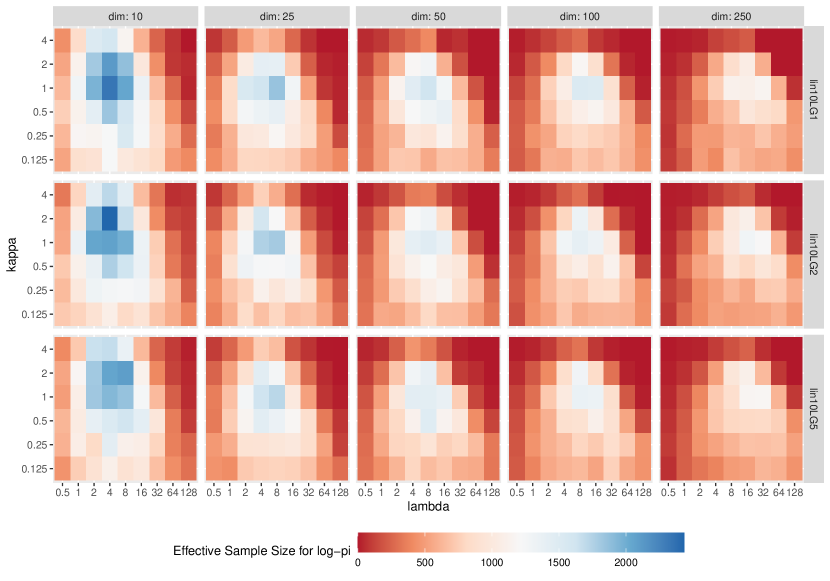
Figure 2: Effective sample size of $\ell(X)$ under Hop on a range of targets (rows) with scales increasing from $1$ to $10$ with dimension index, and dimensions (columns). Within each cell, $\lambda$ and $\kappa$ are varied on an logarithmic scale (base 2).

Hop is designed to move between contours of $\log\pi$. The effective sample size of $\log\pi_{\mathsf{LG}}(X;0,\sigma,a)$ as a function of the choice of $a,d,\lambda,\kappa$ is shown in Figure 1 for i.i.d. targets and in Figure 2 for Linear targets. Firstly, whatever the target, the optimal $\lambda$ increases with dimension just slightly slower than in proportion to $d^{1/2}$. By contrast the optimal $\kappa$ is remarkably stable across targets and dimension, lying between $0.25$ and $1$ for i.i.d. targets and between $1$ and $2$ for linear targets; recall that on a perfectly isotropic target detailed balance could be satisfied with $\kappa=0$ since the gradients at the current and proposed values would align. For each combination of dimension and target, the acceptance rates at the optimal $(\lambda,\kappa)$ values were between 0.1 and 0.46. Moreover, all plots show that the effects of $\lambda$ and $\kappa$ on performance are approximately orthogonal to each other, backing up the reparameterisation from $(\lambda,\mu)$ to $(\lambda,\kappa)$ suggested by Theorem 2.

Finally, Hop efficiency degraded exceptionally slowly with dimension in the i.i.d. case: the ratio of the optimal effective sample size (ESS) with $d=250$ to the optimal ESS with $d=10$ was $0.75$ for ISOLG1, $0.68$ for ISOLG2, and $0.61$ for ISOLG5. In the case of Linear targets, the corresponding ratios were $0.50,0.53,0.56$ indicating a roughly 50% reduction in efficiency when dimension increases by a factor of 25.

2.6 Parallels with Hamiltonian Monte Carlo

We now discuss the similarities and differences between Hug and Hamiltonian Monte Carlo. Both algorithms augment the state space via a velocity $v_{0}$, which is typically drawn from a $\mathsf{N}(0,\Sigma)$ distribution. Hug approximates the movement for time $T$ along a level set of $\pi$ via a series of $B$ reflections, each accounting for an integration time of $\delta=T/B$. Hamiltonian Monte Carlo approximates the Hamiltonian dynamics of a particle moving in a potential of $-\ell$, which is equivalent movement along the level sets of total energy, via $L$ repeats of the Leapfrog integrator (e.g. Neal,, 2011), each of which accounts for a time $\delta=T/L$:

$$v^{\prime}=v_{b}+\frac{\delta}{2}\nabla\ell(x),~{}~{}x_{b+1}=x_{b}+\delta M^{-1}v^{\prime},~{}~{}v_{b+1}=v^{\prime}+\frac{\delta}{2}\nabla\ell(x_{b+1}),$$

where $M=\Sigma^{-1}$ is the positive-definite mass matrix. As with reflections, each leapfrog step is skew reversible with a Jacobian of $1$, and so the kernel targets $\widetilde{\pi}(x,v)=\pi(x)q(v\mid x)$ for exactly the same reasons as Hug does. Also, as with Hug (Theorem 1), the error in $\log\widetilde{\pi}$ after integrating for a fixed time $T$ using steps of size $\delta$ is $\mathcal{O}(\delta^{2})$ (e.g. Leimkuhler et al.,, 2004).

An appropriate choice of $M$ also allows for global preconditioning of Hamiltonian Monte Carlo; however, any scheme that seeks to use local Hessian information to set the mass matrix in the leapfrog step whilst maintaining skew-reversibility must be implicit and, hence, much more time consuming: e.g. the middle step could become: $x_{b+1}=x_{b}+\delta M^{-1}(\{x_{b}+x_{b+1}\}/2)v^{\prime}$ (see also Girolami and Calderhead,, 2011, for an implicit scheme which uses 3rd derivatives of $\ell$). This remains true if the alternative, position-Verlet leaprog method is used. The benefit of using local Hessian information is demonstrated in Section 3 (see also Girolami and Calderhead,, 2011).

The leapfrog step is symplectic and, as a consequence, if $\delta$ is fixed and $\delta v_{0}$ is not too large given the curvature of $\log\pi$, then as $T=L\delta$ increases the quantity $|\ell(x_{L})-\ell(x_{0})|$ remains bounded (e.g. Leimkuhler et al.,, 2004). Hug is not symplectic; nonetheless, we have found empirically that, as with the leapfrog scheme, if $\delta v_{0}$ is not too large compared with the Hessian of $\log\pi$, as $T=B\delta$ increases, $|\ell(x_{B})-\ell(x_{0})|$ remains bounded; Figure 7 in Appendix C.2 demonstrates this empirically for several different targets. A final difference between the algorithms is in robustness to large gradient values, which we document next.

2.7 Ergodicity and convergence

On an isotropic target, neither Hug nor optimally tuned Hop is ergodic, as each algorithm is reducible. By the symmetry of the reflection operation, Hug remains on the same contour of $\log\pi$ forever. By contrast, since $g(y)$ is parallel to $g(x)$, Hop tuned with $\mu=0$ becomes a one-dimensional algorithm along a particular radial line; the same cancellation of large terms occurs, $\lambda$ can still be $o(d^{1/2})$, and the limiting acceptance rate is $1$. Though neither algorithm on its own is ergodic on such a target, Proposition 2 (proved in Appendix F.1) shows that the pair in tandem is. As mentioned in Section 2.5, to avoid issues with very small gradients we replace the $1/||g(x)||^{2}$ term in (4) by $1/\left(1\vee||g(x)||\right)^{2}$.

Proposition 2.

Let the distribution $\pi$ have a density with respect to Lebesgue measure on $\mathbb{R}^{d}$ of $f(||x||)$ for some $f:[0,\infty)\to(0,b)$, $b<\infty$. The Hug and Hop algorithm targeting $\pi$, with Hug using $v_{0}\sim\mathsf{N}(0,\tau^{2}I_{d})$, and with Hop using a proposal as in (4) but with $||g(x)||^{2}$ replaced by $1\vee||g(x)||^{2}$ is ergodic whether or not the $\mu$ scale parameter is zero.

Geometric ergodicity, convergence that is exponential in the number of iterations, is often deemed desirable. The two main classes of obstacles to geometric ergodicity are the existence of one or more regions of the space where the direction to the “centre” is difficult to discern, so the chain meanders (see, for example, Theorem 3.3 of (Mengersen and Tweedie,, 1996) or Theorem 4.3 of (Roberts and Tweedie, 1996a, )), or where the acceptance rate can drop arbitrarily close to $0$ (Roberts and Tweedie, 1996b, , Proposition 5.1). Local algorithms, such as the random-walk Metropolis, the Metropolis-adjusted Langevin algorithm and Hamiltonian Monte Carlo, as well as Hug and Hop, suffer from the former problem when the tails of the target decay slower than exponentially. The latter issue arises in gradient-based algorithms, including the Metropolis-adjusted Langevin algorithm (Roberts and Tweedie, 1996a, , Theorem 4.2)) and Hamiltonian Monte Carlo (Livingstone et al.,, 2019, Theorem 2.2) when the tails of the target are lighter than Gaussian, essentially because each leapfrog step includes two shifts of size $\mathcal{O}(||g(x)||)$, and $||g(x)||$ increases too quickly; however, this need not be an issue for Hug and Hop despite its use of gradients because Hug only depends on $g$ via $\widehat{g}=g/||g||$, and in the presence of large gradients Hop reduces the size of its jump proposals rather than increasing them.

We formally show the robustness of Hop for the class of one-dimensional targets investigated in Roberts and Tweedie, 1996a and Livingstone et al., (2019):

$$\pi(x)\propto\exp\left(-\frac{1}{a}|x|^{a}\right),~{}~{}~{}x\in\mathbb{R}.$$ (12)

For such targets, the random-walk Metropolis is known to be geometrically ergodic for $a\geq 1$ (e.g. Mengersen and Tweedie,, 1996, Theorem 3.2), whereas the Metropolis-adjusted Langevin algorithm (Roberts and Tweedie, 1996a, , Theorems 4.1, 4.2 and 4.3) and Hamiltonian Monte Carlo (Livingstone et al.,, 2019, Corollary 2.3) are both geometrically ergodic only if either $1\leq a<2$, or, subject to an upper bound on the scale parameter, if $a=2$. Theorem 3, which is proved in Appendix F.2, shows that the Hop algorithm is geometrically ergodic on light-tailed targets of the form (12).

Theorem 3.

A Metropolis-Hastings algorithm with a proposal as in (4) but with $||g(x)||^{2}$ replaced by $1\vee||g(x)||^{2}$ is geometrically ergodic on targets of the form (12) provided $a\geq 1$.

We demonstrate empirically the convergence illustrated in Theorem 3 in a broader setting, using a target from Sherlock and Thiery, (2021):

$$\pi(x)\propto\exp\left(-\left|\left|{x}\right|\right|_{M}^{a}/a\right),~{}~{}~{}x\in\mathbb{R}^{d},$$ (13)

where $\left|\left|{x}\right|\right|^{2}_{M}=\sum_{i=1}^{d}x_{i}^{2}/\sigma_{i}^{2}$ and $\bm{\sigma}=(1,\dots,d)$. The mode of $\left|\left|{X}\right|\right|_{M}$ when $X\sim\pi$ is $r^{*}=(d-1)^{1/a}$.

Firstly, we tuned Hamiltonian Monte Carlo and Hug and Hop to the main body of the target in (13) with $d=25$ and $a=4$. This led, respectively, to $(T=2.0,L=4)$ and $(T=1.0,B=5,\lambda=10,\kappa=2)$. Using these tuning parameters, we repeated the following $N=50$ times for $\gamma\in\{1,1.5,2,2.5,3\}$, and each kernel $K\in\left\{{\textrm{Hamiltonian Monte Carlo},\textrm{Hop},\textrm{Hug and Hop}}\right\}$:

• Set $y=z/\left|\left|{z}\right|\right|$, where $z\sim\mathsf{N}_{25}\left(0,I\right)$, so $y$ is uniform on the unit sphere.

• Set the initial condition: $x_{0}=\gamma r^{*}(\sigma_{1}y_{1},\ldots,\sigma_{d}y_{d})$ so that $||x||_{M}=\gamma r^{*}$.

• Run kernel $K$ for 50,000 iterations and record the first time that $\left|\left|{x}\right|\right|_{M}\leq r^{*}$.

At $\gamma=1$, the procedure draws a point at the modal value of $\left|\left|{X}\right|\right|_{M}$; as $\gamma$ increases, the initial value moves further into the tails of the target. The condition $\left|\left|{x}\right|\right|_{M}\leq r^{*}$ is a proxy for convergence from the tails to the posterior modal distance. The results are given in Figure 8 in Appendix G. Even when $\gamma=1.5$, Hamiltonian Monte Carlo fails to accept any proposals during 50,000 iterations and thus never converges by the above condition. In contrast, Hop converges for all values of $\gamma$ considered, with only a slight increase in the time to convergence. Hop uses the gradient in two places: (i) to guide the variance of the proposal which only uses the unit vector in the gradient direction (and is thus not affected by the norm), and (ii) as the scaling of the covariance matrix, which becomes small, not large, when the gradient norm is large.

2.8 Parameter tuning

Hug and Hop have different purposes, respectively to move in $\mathcal{X}$ and to change $\log\pi$, and have separate parameters, respectively $(T,B)$ and $(\lambda,\kappa)$. We recommend tuning the pairs of parameters separately, each with the relevant goal in mind.

For Hug, as with HMC, $T$ should be large enough that a reasonable distance is covered, but not so large that the proposal dynamic is likely to perform a loop, making $||x_{B}-x_{0}||\ll||Tv_{0}||$. Given $T$, $\delta$ should be chosen so that the acceptance rate is bounded away from $0$ and $1$. Empirical studies across a range of toy targets, dimensions and integration times (see Appendix C.1) suggest setting $\delta$ so as to target an acceptance rate of between $60\%$–$85\%$.

Tuning advice for Hop derives from Theorem 2, the discussion thereafter and the simulation study of Section 2.5. With reasonable preconditioning, set $\kappa\in[0.25,1.0]$, perhaps a little larger if the preconditioning is poor. With small $\lambda$ this leads to the acceptance rate in (10). For the chosen $\kappa$, increase $\lambda$ until the asymptotics no longer apply and the acceptance rate starts to decreases rapidly.

3 Simulation study

We now compare the Hug and Hop sampler to various other algorithms on a range of target distributions in $d=25$ dimensions. We consider six classes of Model: (i) A Gaussian distribution with a diagonal co-variance matrix; (ii) a product of a logistic density and a weak, regularising Gaussian density $\pi_{\mathsf{LG}}(x;5,\underline{\sigma})$, as defined in (11); (iii) a product of a “quartic” and a weakly regularising Gaussian:

$$\pi_{\mathsf{QG}}(x;a,\underline{\sigma})\propto\prod_{i=1}^{d}\exp\left[-\frac{1}{4}\left(\frac{x_{i}}{\sigma_{i}}\right)^{4}\right]\exp\left[-\frac{1}{2}\left(\frac{x_{i}}{a\sigma_{i}}\right)^{2}\right]$$ (14)

with $a=3$. Models (iv) - (vi) are more exotic, each consists of a $d=25$ dimensional target with dimensions $1$ and $2$ independent of dimensions $3,\dots,d$, which themselves are independent, centred Gaussians. The first two dimensions are: (iv) the Banana target of (Sejdinovic et al.,, 2014) with bananacity $\lambda=0.95$, (v) a well-separated bimodal mixture of Gaussians and (vi) the Plus-Prism: a mixture of two Gaussians forming a “+”-shaped target. Further details of these targets can be found in Appendix H.

For each target, we consider two types of scaling across the components: Isotropic scales, where the scale parameter of each component is $1$, and Linear scales, where the scale parameter for component $i$ is $1+24\times(d-i)/(d-1)$. This yields $12$ targets.

The following MCMC algorithms were compared: the random walk Metropolis (RWM), both vanilla and with Hessian-based proposal variance (e.g. Sejdinovic et al.,, 2014); the Metropolis-adjusted Langevin algorithm (MALA) (Besag,, 1994; Roberts and Rosenthal,, 1998); simplified manifold MALA (SMMALA, Girolami and Calderhead,, 2011), which is MALA with position-dependent preconditioning; Hamiltonian Monte Carlo; Hug and Hop; Hug and Hop with both proposals using local Hessian information.

For each combination of target distribution and MCMC algorithm, to allow a fair comparison, the algorithm was tuned over a grid of parameter values and the minimum effective sample size over all components of $X$ was found from a run of $50,000$ iterations with the optimal parameter choice. Typically, algorithm runs have a fixed computational budget or time limit, so the total computational time for each run was also noted and efficiency was measured in terms of the minimum effective sample size per second. To compare the samplers, we consider values within each model relative to the best for that model.

The results, presented in Figure 3, show that for unit targets Hug and Hop and Hamiltonian Monte Carlo are the most efficient samplers, and for linear targets Hug and Hop using position-dependent preconditioning is most efficient. The only exception is the linear banana, where the standard Hug and Hop and Hamiltonian Monte Carlo are more efficient than Hug and Hop using position-dependent preconditioning.

The superiority of Hug and Hop on the bimodal target is of particular interest, and so we compare it, Hamiltonian Monte Carlo and the No U-turn Sampler of Hoffman and Gelman, (2014), all without preconditioning, in a bimodal target stretched so that movement between modes happens only rarely. We tuned to obtain the maximum frequency of flips from one mode to the other taking CPU cost into account. The target and example trace plots are provided in Appendix H.2, along with detailed results. In summary, in this experiment, Hug and Hop is about $1.5$ times as efficient as Hamiltonian Monte Carlo, which is over twice as efficient as the No U-turn Sampler.

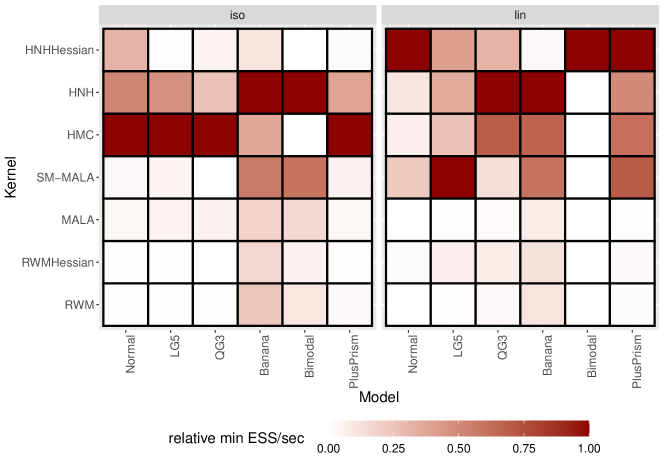
Figure 3: Minimum effective size (ESS) over the components of $x$ per wall-clock second. Each sampler/target pair was run for 50,000 iterations on a 25- dimensional target. Values are relative to the most efficient algorithm within each model (columns).

In general targets, Hessian calculations have a cost of $\mathcal{O}(d^{2})$. As dimension increases, use of position-dependent conditioning would only remain of benefit if the eccentricity of the contours also increased sufficiently quickly, or the position-dependent conditioning was cheap to compute.

4 Statistical models

In this section the utility of Hug and Hop is demonstrated and compared against Hamiltonian Monte Carlo on some some real-world models, using simulated data: $30$- and $100$-dimensional Cauchit regression models; an item-response, or Rash, model with $20$ tests and $100$ subjects; and a 1002-dimensional stochastic volatility model. In the first two examples, we also test the No U-turn Sampler of Hoffman and Gelman, (2014), where the recursive tree building leads to additional computational expense, so performance is measured in effective samples per CPU second. For the other example performance is evaluated via effective samples per gradient evaluation since gradient evaluations are by far the most computationally expensive operations performed each iteration. For fairness of comparison and to enable verification of our tuning advice, algorithms were tuned for maximum efficiency across a grid of parameter values as in Section 3.

4.1 Cauchit regression

For data consisting of binary responses with covariate information, the logistic or probit link functions are popular choices for the Bernoulli GLM, but these link functions are not robust to outliers where the linear predictor is large in absolute value, indicating the outcome is almost certain, but the linear predictor is wrong (Koenker and Yoon,, 2009). Such a situation may arise from errors in the data-recording process, for example. The “Cauchit” link function is more tolerant of such outliers. The model supposes that the $i$th binary response, $Y_{i}$ is related to the vector of $M$ predictors for the response, $x_{i}$, through some unknown parameters, $\beta$, as follows:

$$Y_{i} \stackrel{{\scriptstyle\mathrm{indep.}}}{{{\sim}}}\mathsf{Bernoulli}(p_{i}),\text{ for }i=1,\ldots,N$$ (15)

$$g(p_{i}) \overset{\textrm{iid}}{\sim}\beta^{\top}x_{i},~{}\mbox{where}~{}g({u})=\tan(\pi(u-1/2)),$$

$$\beta_{j} \overset{\textrm{iid}}{\sim}\mathsf{N}\left(0,1/\tau\right),\text{ for }i=1,\ldots,M.$$

We simulated $M=30$ coefficients, $\beta_{1},\dots,\beta_{M}$, from (15) with $\tau=1$, and $N=1000$ data points, $Y_{i}$, $i=1,\ldots,N$, using predictors ($x_{i,1},\ldots,x_{i,M}$), each of which was independently drawn from a $\mathsf{N}\left(0,1\right)$ distribution. We compared the three algorithms on a posterior from (15) with $\tau=1$, starting each algorithm at the true parameter value and running for 50,000 iterations. We then repeated the simulation and analysis but with $M=100$. For extra robustness, both Hamiltonian Monte Carlo and Hug use jittering similar to that in Neal, (2011): at each iteration, simulate $T^{*}\sim\mathsf{Unif}[0.8T,1.2T]$, then, respectively set $\epsilon=T^{*}/L$ or $\delta=T^{*}/B$.

With $M=30/100$, the optimal tunings were: $\epsilon=0.11/0.08$ for the No U-turn Sampler, which led to a mean number of leapfrogs per iteration of $\approx 7.08/14.91$; $(T,L)=(0.5,5)/(0.8,14)$ for Hamiltonian Monte Carlo and $(T,B,\lambda,\kappa)=(0.7,6,12,0.5)/(0.8,11,12,0.5)$ for Hug and Hop. Table 1 provides the acceptance rates and efficiencies at these tunings. For $M=30$, Hug and Hop is slightly more efficient than Hamiltonian Monte Carlo, whereas with $M=100$ Hamiltonian Monte Carlo is around $50\%$ more efficient. In each case, both are more efficient than the The No U-turn Sampler.

Kernel	HMC	Hug and Hop	NUTS
$\alpha$ ($M=30$)	71.6	74.6, 33.5	88.8
Efficiency ($M=30$)	4630	5108	3248
$\alpha$ ($M=100$)	86.1	72.4, 36.3	94.8
Efficiency ($M=100$)	1565	952	853

Table 1: Acceptance rates and efficiency for the three algorithms on the Cauchit regression model with $N=1000$ and $M\in\{30,100\}$. Efficiency is measured in terms of the minimum over components of the effective sample size per 1000 CPU seconds.

4.2 Rasch model

Consider a set of $N$ true or false questions answered by $M$ people. Let $Y_{ij}=1$ if person $i$ answered question $j$ correctly, and $Y_{ij}=0$ otherwise. The Rasch model (Rasch,, 1980) posits that the $j$-th question has some latent difficulty $\beta_{j}$ and the $i$-th person has a latent ability $\eta_{i}$ such that the probability person $i$ is correct when answering question $i$ is given by $P_{ij}=\Phi(\eta_{i}-\beta_{j})$, where $\Phi$ is the distribution function of a standard Gaussian. Each answer $Y_{ij}$ is thus considered as a Bernoulli outcome with probability $P_{ij}$. Model identifiability can be ensured by arbitrarily fixing one of the parameters to $0$; however, there is no a priori reason to believe this of any of the parameters. Our Bayesian analysis sidesteps the issue, keeping the exchangeability of the original model and ensures identifiability via the prior; we also do this as it increases the correlation between the parameters, making the problem more challenging. The model is:

$$Y_{ij} \stackrel{{\scriptstyle indep.}}{{{\sim}}}\mathsf{Bernoulli}\left(\Phi(\eta_{i}-\beta_{j})\right),$$ (16)

$$\eta_{i} \overset{\textrm{iid}}{\sim}\mathsf{N}\left(0,\tau^{-1}\right)\text{ for }i=1,\ldots,M,$$

$$\beta_{j} \overset{\textrm{iid}}{\sim}\mathsf{N}\left(0,\tau^{-1}\right)\text{ for }i=1,\ldots,N.$$

We simulated data from the model (16) with $M=100$ people, $N=20$ tests and $\tau=1$. For the subsequent inference on $\theta=(\eta_{1},\dots,\eta_{M},\beta_{1},\dots,\beta_{N})$, the priors for $\eta_{i}$ and $\beta_{j}$ were as in the model (16).

A diagonal preconditioning matrix was used: $\Sigma=\mathsf{diag}(1,\dots,1,N/M,\dots,N/M)$, where the last $N=20$ elements are $N/M=0.2$. Hamiltonian Monte Carlo used a mass matrix of $M=\Sigma^{-1}$. Each sampler was run for 50,000 iterations, with jittering of $T$ applied as in Section 4.1.

The optimal tunings were $\epsilon=0.25$ for the No U-turn sampler, which led to a mean number of leapfrog steps per iteration of $7.01$, $(T,L)=(1.0,5)$ for Hamiltonian Monte Carlo, and $(T,B,\lambda,\kappa)=(1.2,5,15,0.25)$ for Hug and Hop. The results are given in Table 2 and show that Hamiltonian Monte Carlo and Hug and Hop have similar performance. Even though the former performs better on $\eta$, Hug and Hop performs better on the worst mixing component, which is a component of $\beta$.

Kernel	HMC	Hug and Hop	NUTS
$\alpha$ (%)	79.2	86.6, 48.6	89.0
Efficiency($\eta$)	235	215	150
Efficiency($\beta$)	105	121	78

Table 2: The Rasch model with $M=100$ and $N=20$: acceptance rates and efficiencies for the three algorithms. Efficiency both for the vector $\eta$ and the vector $\beta$ is measured in terms of the minimum over the vector of the effective sample size per CPU second.

4.3 Stochastic Volatility Model

Consider the following model for zero-centred data $y=(y_{0},\dots,y_{T-1})$ where the variance depends on a zero-mean, Gaussian AR(1) process started from stationarity:

$$y_{t} \sim\mathsf{N}\left(0,\frac{\exp(2x_{t})}{\tau}\right),~{}t=0,\dots,T-1,$$

$$x_{0} =\frac{z_{0}}{\phi}~{}~{}~{}\mbox{and}~{}~{}~{}x_{t}=\rho x_{t-1}+z_{t},~{}t=1,\dots,T-1,$$

where $z_{t}\sim\mathsf{N}(0,1),~{}t=0,\dots,T-1$ are iid. Parameter priors are $\tau~{}\sim\mathsf{Gamma}(21,5)$ and $(1+\rho)/2\sim\mathsf{Beta}(20,2)$, with $\phi=\sqrt{1-\rho^{2}}$. Standard transformations ensure that all parameters have support on $(-\infty,\infty)$:

$$\alpha=-\frac{1}{2}\log(\tau),\quad\beta=\frac{1}{2}\left\{\log(1+\rho)-\log(1-\rho)\right\}.$$

Appendix I.3 provides the log posterior and its gradients with respect to $z$, $\alpha$ and $\beta$.

We simulated data from the model using the parameters $(\tau,\rho)=(4.0,0.95)$ (see Figure 11 in Appendix I.3). We then ran HMC with $T=3.0,L=35$ and Hug and Hop with $T=3.75,B=35,\lambda=10,\kappa=0.5$. In each case a diagonal pre-conditioning matrix estimated from some initial runs was used. For Hug and Hop, the Hop kernel was applied five times per iteration, rather than once, as this was found to improve the mixing at little extra computational cost.

Each sampler was initialised at a point well supported by the posterior and run for 50,000 iterations. HMC uses 35 steps and thus 35 gradient evaluations per iteration. For hug and hop, hug uses 35 evaluations and hop (repeated five times) uses 5, giving a total of 40. The acceptance rates were 87% for HMC, 77% for Hug, and 39% for Hop. The worst mixing component was $\beta$, for which Hamiltonian Monte Carlo is slightly more efficient than Hug and Hop.

Kernel	HMC	Hug and Hop
Acceptance rate $\alpha$	0.87	0.77, 0.39
Efficiency ($\alpha$)	2755	2410
Efficiency ($\beta$)	598	523
Efficiency ($Z$)	1600	1400

Table 3: Stochastic Volatility model with $T=1000$: acceptance rates and efficiencies for $\alpha$, $\beta$ and the vector $Z$. Efficiency is measured in terms of the (minimum, for $Z$) effective sample size per 50000 gradient evaluations.

Appendix A Additional algorithm details

One iteration of the full Hug-and-Hop algorithm with a symmetric proposal density $q(v|x)$ for Hug and with the Hop proposal robust to small gradient magnitudes proceeds as follows:

• Hug time, $T$; Hug # steps, $B$; Hop scale, $\lambda$; Hop ratio $\kappa$; current value, $x$.

• $x_{0}\longleftarrow x$ and $\delta\longleftarrow T/B$.

• Draw velocity $v_{0}\sim q(\cdot|x_{0})$ .

• For $b=0,\ldots,B-1$,

  • Move to $x_{b}^{\prime}=x_{b}+\delta v_{b}/2$.

  • Reflect: $v_{b+1}\longleftarrow~{}\mathsf{R}\left({v_{b};g(x_{b}^{\prime})}\right)$.

  • Move to $x_{b+1}=x_{b}^{\prime}+\delta v_{b+1}/2$.

• EndFor

• Compute $\log r_{hug}=\ell(x_{B})-\ell(x_{0})+\log q(v_{B}|x_{B})-\log q(v_{0}|x_{0})$.

• With a probability of $\alpha_{hug}=1\wedge r_{hug}$, $x\longleftarrow x_{B}$; otherwise $x\longleftarrow x$.

• Draw $y$ from $\mathsf{N}\left(x,\frac{1}{1\vee||g(x)||^{2}B_{x}}\right)$, where $B_{x}=\lambda\kappa I+(\lambda^{2}-\lambda\kappa)\widehat{g}(x)\widehat{g}(x)^{\top}$.

• Set $B_{y}=\lambda\kappa I+(\lambda^{2}-\lambda\kappa)\widehat{g}(y)\widehat{g}(y)^{\top}$ and compute

  $$\log r_{hop}=\ell(y)-\ell(x)+\log\mathsf{N}\left(x;y,\frac{B_{y}}{1\vee\left|\left|{g(y)}\right|\right|^{2}}\right)-\log\mathsf{N}\left(y;x,\frac{B_{x}}{1\vee\left|\left|{g(x)}\right|\right|^{2}}\right).$$

• With a probability of $\alpha_{hop}=1\wedge r_{hop}$, $x\longleftarrow y$; otherwise $x\longleftarrow x$.

In practice, in the above we often choose $q(v|x)$ to be $\mathsf{N}\left(v;0,I_{d}\right)$ so that the two $\log q$ terms in $r_{hug}$ cancel. When per-iteration jittering is used in Hug, the first line of Hug changes to $x_{0}\longleftarrow x$, $T_{*}\sim\mathsf{Unif}[0.8T,1.2T]$ and $\delta=T_{*}/B$. When pre-conditioning is used, the whole algorithm applies to the transformed posterior.

The hug algorithm with position dependent conditioning is given below. In practise we choose $q(v|x)$ to be $\mathsf{N}\left(v;0,\Sigma(x)\right)$.

• Require: integration time, $T$; # steps, $B$; current value, $x$; position dependent scaling function $\Sigma(x)$.

• $x\longleftarrow x_{0}$ and $\delta\longleftarrow T/B$.

• Draw velocity $v_{0}\sim q(\cdot|x_{0})$ .

• For $b=0,\ldots,B-1$

  • Move to $x_{b}^{\prime}=x_{b}+\delta v_{b}/2$.

  • Reflect: $v_{b+1}\longleftarrow v_{b}-2\frac{v_{b}^{\top}g(x)}{g(x)^{\top}\Sigma(x)g(x)}\Sigma(x)g(x)$.

  • Move to $x_{b+1}=x_{b}^{\prime}+\delta v_{b+1}/2$.

• EndFor

• Compute $\log r_{hug}=\ell(x_{B})-\ell(x_{0})+\log q(v_{B}|x_{B})-\log q(v_{0}|x_{0})$.

• With a probability of $\alpha_{hug}=1\wedge r_{hug}$, $x\longleftarrow x_{B}$; otherwise $x\longleftarrow x$.

Appendix B Proofs of Theoretical results for Hug

B.1 Proof of Theorem 1

In this section we prove Theorem 1.

Proof.

Firstly, write the difference in $\ell$ at $x_{B}$ and $x_{0}$ as a telescoping sum and apply Equation (2):

$$\ell(x_{B})-\ell(x_{0}) =\sum_{b=1}^{B}\ell(x_{b})-\ell(x_{b-1})$$ [telescope]

$$=\frac{\delta^{2}}{8}\sum_{b=1}^{B}\left[v_{b}^{\top}H(x_{b}^{-})v_{b}-v_{b-1}^{\top}H(x_{b-1}^{+})v_{b-1}\right]$$ [Equation (2)]

$$=\frac{\delta^{2}}{8}\left(v_{B}^{\top}H(x_{B}^{-})v_{B}-v_{0}^{\top}H(x_{0}^{+})v_{0}+\sum_{b=1}^{B-1}\left[v_{b}^{\top}(H(x_{b}^{-})-H(x_{b}^{+}))v_{b}\right]\right)$$ (17)

Recall that $x_{b}^{-}$ and $x_{b}^{+}$ lie on the line segment, namely the segment joining the bounce points $x_{b-1}^{\prime}$ and $x_{b}^{\prime}$. Furthermore, note that $x_{b}^{\prime}=x_{b}+\delta v_{b}/2=x_{b-1}^{\prime}+\delta v_{b}$, therefore:

$$\left|\left|{x_{b}^{+}-x_{b}^{-}}\right|\right|\leq\left|\left|{x_{b}^{\prime}-x_{b-1}^{\prime}}\right|\right|=\delta\left|\left|{v_{i}}\right|\right|.$$

This allows us to bound each term in the summation within (17):

$$|v_{b}^{\top}(H(x_{b}^{-})-H(x_{b}^{+}))v_{b}| \leq\left|\left|{v_{b}}\right|\right|\left|\left|{(H(x_{b}^{-})-H(x_{b}^{+}))v_{b}}\right|\right|$$ [Cauchy-Shwartz]

$$\leq\left|\left|{v_{b}}\right|\right|^{2}\left|\left|{H(x_{b}^{-})-H(x_{b}^{+})}\right|\right|_{I}$$ [Definition of induced norm]

$$\leq\gamma\left|\left|{v_{b}}\right|\right|^{2}\left|\left|{x_{b}^{+}-x_{b}^{-}}\right|\right|$$ [Condition 1]

$$\leq\gamma\delta\left|\left|{v_{b}}\right|\right|^{3}.$$ (18)

By Condition 2, we can also bound the first difference in (17):

$$v_{B}^{\top}H(x_{B}^{-})v_{B}-v_{0}^{\top}H(x_{0}^{+})v_{0}\leq\beta(\left|\left|{v_{B}}\right|\right|^{2}+\left|\left|{v_{0}}\right|\right|^{2})=2\beta\left|\left|{v_{0}}\right|\right|^{2},$$ (19)

where we use the fact $\left|\left|{v_{b}}\right|\right|=\left|\left|{v_{b-1}}\right|\right|$ since reflection preserves the norm. Combining (18) and (19) in (17) with the triangle inequality results in:

$$|\ell(x_{B})-\ell(x_{0})| \leq\frac{\delta^{2}}{8}\left[\left|{v_{B}^{\top}H(x_{B}^{-})v_{B}-v_{0}^{\top}H(x_{0}^{+})v_{0}}\right|+\left|{\sum_{b=1}^{B-1}v_{b}^{\top}(H(x_{b}^{-})-H(x_{b}^{+}))v_{b}}\right|\right]$$

$$\leq\frac{\delta^{2}}{8}\left(2\beta\left|\left|{v_{0}}\right|\right|^{2}+(B-1)\gamma\delta\left|\left|{v_{0}}\right|\right|^{3}\right)$$

$$\leq\frac{\delta^{2}\left|\left|{v_{0}}\right|\right|^{2}}{8}\left(2\beta+\gamma\left|\left|{Tv_{0}}\right|\right|\right),$$

where the last line follows from $T=B\delta$. ∎

B.2 Proof of Proposition 1

Proof.

Without loss of generality, set $b=0$ and write $A$ for $A(x_{0}^{\prime})$. Applying (2) but in the transformed space where the Hessian is $\widetilde{H}(x)=AH(\widetilde{x})A^{\top}$, gives

$$|\ell(x_{1})-\ell(x_{0})| =|\ell(\widetilde{x}_{1})-\ell(\widetilde{x}_{0})|$$

$$=\frac{\delta^{2}}{8}\left|{\widetilde{v}_{1}^{\top}AH(x_{1}^{\prime})A^{\top}\widetilde{v}_{1}-\widetilde{v}_{0}^{\top}AH(x_{0}^{\prime})A^{\top}\widetilde{v}_{0}}\right|$$

$$\leq\frac{\delta^{2}}{8}\left|{\widetilde{v}_{1}^{\top}AH(x^{\prime})A^{\top}\widetilde{v}_{1}-\widetilde{v}_{0}^{\top}AH(x^{\prime})A^{\top}\widetilde{v}_{0}}\right|$$

$$~{}~{}~{}~{}+\frac{\delta^{2}}{8}\left|{\widetilde{v}_{1}^{\top}A[H(x_{1}^{\prime})-H(x^{\prime})]A^{\top}\widetilde{v}_{1}-\widetilde{v}_{0}^{\top}A[H(x_{0}^{\prime})-H(x^{\prime})]A^{\top}\widetilde{v}_{0}}\right|$$

$$=\frac{\delta^{2}}{8}\left|{v_{1}^{\top}[H(x_{1}^{\prime})-H(x^{\prime})]v_{1}-v_{0}^{\top}[H(x_{0}^{\prime})-H(x^{\prime})]v_{0}}\right|$$

$$\leq\frac{\gamma\delta^{3}}{8}\left\{\left|\left|{v_{1}}\right|\right|^{3}+\left|\left|{v_{0}}\right|\right|^{3}\right\}.$$

Here, the third line follows from the triangle inequality, the penultimate line from the fact that $AH(x^{\prime})A=I_{d}$ and $\left|\left|{\widetilde{v}_{1}}\right|\right|=\left|\left|{\widetilde{v}_{2}}\right|\right|$, and the final line since $v^{\top}[H(b)-H(a)]v\leq\gamma\left|\left|{b-a}\right|\right|\left|\left|{v}\right|\right|^{2}$. ∎

Appendix C Empirical exploration of the efficiency of Hug

C.1 Optimal acceptance rate

We explore the relationship between the efficiency of Hug and the acceptance rate by taking a grid of values for $T=0.5,1\to 5$ and $B=1,\ldots,20$ on some example models in dimensions 25, 50, 75 and 100. For each value of the tuple (Model, dimension, $B$, $T$), the following procedure was performed for $i=1\to 10,000$:

1. draw a value for $x_{i}$ directly from the target;

2. apply Hug with parameters $B$, $T$ to obtain $x_{i}^{\prime}$;

3. record $N_{i}=\left|\left|{x_{i}^{\prime}-x_{i}}\right|\right|$ and $\alpha_{i}=\alpha(x_{i}^{\prime},x_{i})$.

Figure 4 shows the efficiency of Hug by plotting $\hat{\mathbb{E}}[AN^{2}]/(dB)$ against acceptance rate $\alpha$; the y-axis approximates the efficiency per unit time since the computational effort for an iteration is essentially proportional to $B$; scaling by $d$ is to compensate for the fact that when $x$ has $d$ components, $\left|\left|{x}\right|\right|^{2}\propto d$.

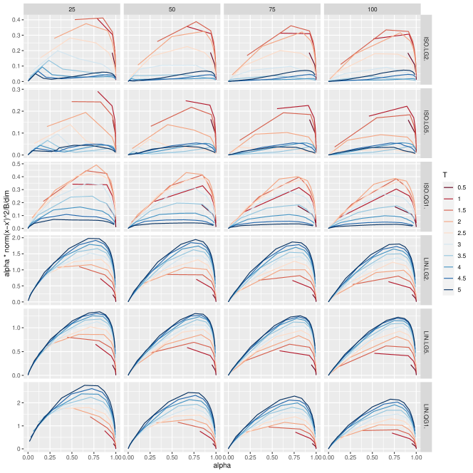
Figure 4: Efficiency plots for Hug: $\alpha$ vs $\mathbb{E}\left[{\alpha\left|\left|{X^{\prime}-X}\right|\right|^{2}}\right]/dB$ for a range of $B$s (each line) on some example models (rows) in increasing dimensions(columns). For Isotropic targets $\sigma=1$ and for LIN targets $\sigma_{i}=1\to 10$. The forms for LG and QG targets can be found in Equation (11) and (14) resp.

C.2 Stability of hug

We first describe a scenario which can be problematical for Hug, then explore a range of more typical scenarios.

In the following two-dimensional target the norms of the gradient and Hessian increase without bound as $||x||\rightarrow\infty$, contravening Conditions 1 and 2 of Theorem 1:

$$\log\pi(x)=-\frac{1}{8}\left\{x_{1}^{8}+\left(\frac{x_{2}}{2}\right)^{8}\right\}+\mbox{constant}.$$ (20)

The relatively sharp “corners”, where the curvature suddenly increases cause problems for Hug. The top row of Figure 5 shows that when $\delta$ is sufficiently small, the behaviour at any given contour can be controlled. This value of $\delta$ is much smaller than is necessary for good behaviour on the “sides” of the contours, which suggests increasing it; however, doubling $\delta$ leads to an unexpected path and a proposal that is very unlikely to be accepted.

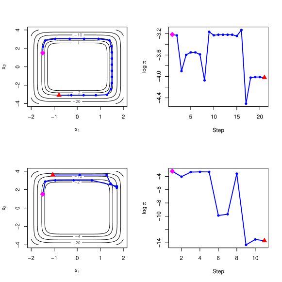
Figure 5: Left: two paths from the Hug algorithm on the target (20), started at $(-1.5,1.5)$ (magenta diamond) with the same initial velocity drawn from $\mathsf{N}(0,I_{2})$ and ending after $T=10$ time units (red triangle). Right: the corresponding values of $\log\pi$ at each point on the path. The top row corresponds to $B=20$ and the bottom row to $B=10$.

To investigate this further, we created a $d=25$-dimensional target with:

$$\log\pi_{8}(x)=-\frac{1}{8}\sum_{i=1}^{d}\frac{x_{i}^{8}}{\sigma_{i}^{8}}+\mbox{constant},$$

and the scales $\sigma_{i}=1+2(i-1)/(d-1)$ and ran Hug for $T=4.0$ with $\delta$ ranging from $0.04$ to $0.8$. We started each run from a random point in the main posterior mass and noted the acceptance rate for Hug each time. The Hop parameters, $(\lambda,\kappa)$ were set to sensible values of $(0.5,1)$, which led to an acceptance rate for Hop of $\approx 40\%$, but no effort was made to tune them.

The black curve in Figure 6 shows how the acceptance rate for Hug plummets as $\delta$ is increased. For comparison, we also ran Hug and Hop on the Targets $\pi_{G}$ (Gaussian) and $\pi_{LG}$ and $\pi_{QG}$ of Section 3 but with the same set of $\sigma_{i}$ as here, and using the same tuning parameters as here but with the largest $\delta$, $0.8$. Even though the target scales are similar, because of the lack of sharp corners, especially with the first two targets, the acceptance rates were much higher: respectively, 94.4%, 97.5% and 63.0%. The quartic terms in the third target caused some deterioriation.

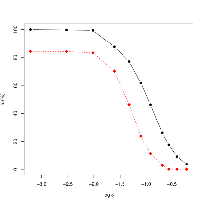
Figure 6: The empirical acceptance rate of Hug (solid, black curve) for various values of $\delta$, with $(T,\lambda,\kappa)=(4,1,0.5)$, and Hamiltonian Monte Carlo (dotted, red curve) for the same $\epsilon\equiv\delta$ values with $T=4$.

Hamiltonian Monte Carlo suffers even more drastically in this situtation. With $(T,\delta)=(4.0,0.8)$, the acceptance rates for the Targets $\pi_{G}$ (Gaussian) and $\pi_{LG}$ and $\pi_{QG}$ were respectively, 91.1%, 95.2% and 37.8%, indicating that this is again a reasonable scaling, but that performance is more substantially reduced when the target has quartic terms and the hints of corners start to appear. The dotted, red curve in Figure 6 shows the acceptance rate for Hamiltonian Monte Carlo applied to $\pi_{8}$ using the set of $\delta$ values also used for Hug. Not only does the acceptance rate reduce to effectively zero much earlier, but no matter how small $\delta$ is, the acceptance rate cannot be increased above about 84%. Much of the posterior for the $i$th component is contained within $[-1.5\sigma_{i},1.5\sigma_{i}]$, but at the edges of this range the magnitude of the gradient is $1.5^{7}/\sigma_{i}\approx 17/\sigma_{i}$. For the lower $\sigma_{i}$ the Leapfrog scheme will only produce a sensible path if the velocity component in these directions is small. As discussed in Section 2.7, Hug only depends on the direction of the gradient, not its magnitude and so, is relatively stable compared with this behaviour.

Figure 7 shows a plot of $\ell(x_{b})-\ell(x_{0})$ against iteration number $b$ of the inner loop in Hug algorithm for a range of 25-dimensional models (definitions for which can be found in the main article, Section 3). Iso models have all scales equal to 1 while Rand models have scales simulated from U(1, 5). The limits on the $y$-axis are chosen as double the maximum and minimum of $\ell(x_{b})-\ell(x_{0})$.

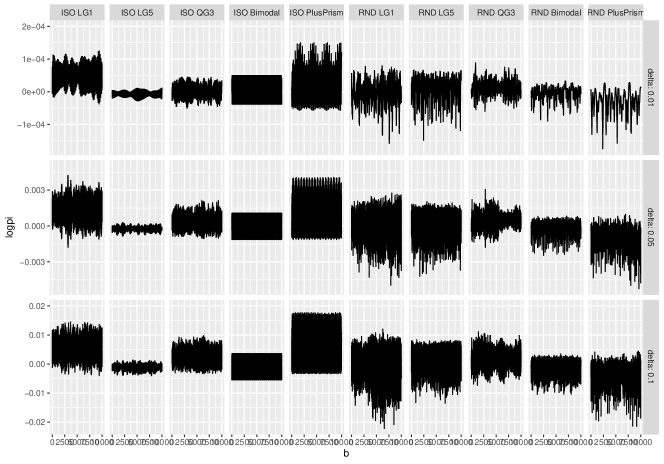
Figure 7: Stability of $\ell$ for various 25-dimensional models (columns) under the Hug algorithm with $\delta=0.01,0.05$ and $0.1$ (rows). Each plot shows $\Delta_{i}=\ell(x_{i})-\ell(x_{0})$ vs. $i=0\to 10,000$.

Appendix D Additional material for Hop

The inverse and square-root of $B_{x}$ are as follows:

$$B_{x}^{-1} =\frac{1}{\mu^{2}}I+\left(\frac{1}{\lambda^{2}}-\frac{1}{\mu^{2}}\right)\widehat{g}(x)\widehat{g}(x)^{\top},$$ (21)

$$B_{x}^{1/2} =\mu I+(\lambda-\mu)\widehat{g}(x)\widehat{g}(x)^{\top}.$$ (22)

For the standard version of Hop, the acceptance ratio in (5) simplifies to:

$$\log r_{hop}(x,y) =\ell(y)-\ell(x)+\log\mathsf{N}\left(x;y,B_{y}/\left|\left|{g(y)}\right|\right|^{2}\right)-\log\mathsf{N}\left(y;x,B_{x}/\left|\left|{g(x)}\right|\right|^{2}\right)$$

$$=\ell(y)-\ell(x)+\frac{d}{2}\log\frac{\left|\left|{g(y)}\right|\right|^{2}}{\left|\left|{g(x)}\right|\right|^{2}}-\frac{1}{2}\left(y-x\right)^{\top}\left[\left|\left|{g(y)}\right|\right|^{2}B_{y}^{-1}-\left|\left|{g(x)}\right|\right|^{2}B_{x}^{-1}\right]\left(y-x\right),$$

$$=\ell(y)-\ell(x)+\frac{d}{2}\log\frac{\left|\left|{g(y)}\right|\right|^{2}}{\left|\left|{g(x)}\right|\right|^{2}}-\frac{1}{2\mu^{2}}\left|\left|{y-x}\right|\right|^{2}\left[\left|\left|{g(y)}\right|\right|^{2}-\left|\left|{g(x)}\right|\right|^{2}\right]$$

$$\qquad-\frac{1}{2}\left(\frac{1}{\lambda^{2}}-\frac{1}{\mu^{2}}\right)\left\{[\left(y-x\right)^{\top}\!g(y)]^{2}-[\left(y-x\right)^{\top}\!g(x)]^{2}\right\}.$$ (23)

using (21), and since $\mathsf{det}(B_{x})=\lambda\mu^{d-1}$ is independent of $x$.

For position-specific preconditioning of Hop, $\left|\left|{\tilde{g}(x)}\right|\right|^{2}=g(x)^{\top}\Sigma(x)g(x)$ and the algorithm proposes points:

$$Y|X=x\sim\mathsf{N}\left(x,\frac{1}{g(x)^{\top}\Sigma(x)g(x)}\left(\mu^{2}\Sigma(x)+(\lambda^{2}-\mu^{2})\frac{\Sigma(x)g(x)g(x)^{\top}\Sigma(x)^{\top}}{g(x)^{\top}\Sigma(x)g(x)}\right)\right)$$ (24)

For a proposed point $y$ from $x$, the log-acceptance ratio for a Hop using Hessian information is:

$$\log r_{hopH} =\ell(y)-\ell(x)+\frac{d}{2}\log\frac{\left|\left|{\tilde{g}(y)}\right|\right|^{2}}{\left|\left|{\tilde{g}(x)}\right|\right|^{2}}+\frac{1}{2}\log\frac{\det{\Sigma(x)}}{\det{\Sigma(y)}}$$

$$\quad-\frac{1}{2\mu^{2}}\left(y-x\right)^{\top}\left(\left|\left|{\tilde{g}(x)}\right|\right|^{2}H_{x}-\left|\left|{\tilde{g}(y)}\right|\right|^{2}H_{y}\right)\left(y-x\right)$$ (25)

$$\quad-\frac{1}{2}\left(\frac{1}{\lambda^{2}}-\frac{1}{\mu^{2}}\right)\left([\left(y-x\right)^{\top}g(y)]^{2}-[\left(y-x\right)^{\top}g(x)]^{2}\right)$$

Appendix E Proof of Theorem 2

E.1 Notation and definitions

In proving Theorem 2 we drop the superscript ^(d) from $\pi^{(d)}$ and $x^{(d)}$ and the subscript from $\lambda_{d}$ and $\mu_{d}$ whenever this is clear from the context. Let $\ell=\log\pi$, $g=\nabla\ell$, $g_{1}=\ell_{1}^{\prime}$ and for $X$ with a density of $\exp(\ell_{1})$, define

$$m_{2} =\mathbb{E}\left[{g_{1}(X)^{2}}\right]=\mathbb{E}\left[{-g_{1}^{\prime}(X)}\right].$$

We switch between the following equivalent forms for the proposed jump vector:

$$y-x=\frac{1}{||g(x)||}(\lambda z^{\parallel}+\mu z^{\bot})=\frac{1}{||g(x)||}\{(\lambda-\mu)z^{\parallel}+\mu z\},$$

where $Z\sim\mathsf{N}(0,I_{d})$ and $Z^{\parallel}=\{\widehat{g}(x)^{\top}Z\}\widehat{g}(x)$ is a $\mathsf{N}(0,1)$ variable along the $\widehat{g}(x)$ vector and $z^{\bot}=z-z^{\parallel}$. Clearly $||z^{\bot}||=\mathcal{O}(d^{1/2})$, whereas $||z^{\parallel}||=\mathcal{O}(1)$.

Further, for $U\sim\mathsf{N}(0,1)$ we define $e_{a}:=\mathbb{E}\left[{|U|^{a}}\right]$ and $v_{a}:=\mathsf{Var}\left[{|U|^{a}}\right]$.

Throughout, ”$\to$” indicates convergence in probability when associated with a sequence of random variables. Also, for a sequence of random variables $A_{d}$ and a sequence of real numbers $b_{d}$, we write $A_{d}\sim b_{d}$ iff $A_{d}/b_{d}\to 1$ and $A_{d}\lesssim b_{d}$ iff $A_{d}/b_{d}\to c$ for some $c\in[0,1]$.

It is natural to split the log acceptance ratio (23) into four terms:

$$C_{1} =\ell(y)-\ell(x)$$

$$C_{2} =\frac{d}{2}\log\frac{||g(y)||^{2}}{||g(x)||^{2}},$$

$$C_{3} =-\frac{1}{2\mu^{2}}||y-x||^{2}\left\{||g(y)||^{2}-||g(x)||^{2}\right\},$$

$$C_{4} =-\frac{1}{2}\left(\frac{1}{\lambda^{2}}-\frac{1}{\mu^{2}}\right)\left[\left\{(y-x)^{\top}g(y)\right\}^{2}-\left\{(y-x)^{\top}g(x)\right\}^{2}\right]=C_{4}^{a}C_{4}^{b},$$

where

$$C_{4}^{a}=(y-x)^{\top}~{}\frac{g(y)+g(x)}{2}.$$

and

$$C_{4}^{b}=-\left(\frac{1}{\lambda^{2}}-\frac{1}{\mu^{2}}\right)(y-x)^{\top}\{g(y)-g(x)\}.$$

The typical sizes of all four terms increase without bound as $d$ increases. However, note that

$$C_{2}=\frac{d}{2}\log\left\{1+\frac{||g(y)||^{2}-||g(x)||^{2}}{||g(x)||^{2}}\right\}\approx\frac{d}{2}\frac{||g(y)||^{2}-||g(x)||^{2}}{||g(x)||^{2}}$$

and

$$C_{4}^{a}\approx\ell(y)-\ell(x).$$

We will show that $C_{2}$ and $C_{3}$ cancel except for terms vanishingly small in $d$, and that the only non-vanishing remainder from $C_{1}+C_{4}$ is $\mathcal{O}(1)$ and leads to the stated acceptance ratio.

E.2 Elementary results

We first gather together some elementary results that will be used repeatedly.

Proposition 3.

$$\mathbb{E}\left[{Z^{\parallel}_{i}Z_{i}}\right]=\frac{g_{1}(x_{i})^{2}}{||g(x)||^{2}}=\mathbb{E}\left[{(Z^{\parallel}_{i})^{2}}\right],$$

$$\mathbb{E}\left[{Z^{\parallel}_{i}Z_{i}^{2}}\right]=\mathbb{E}\left[{(Z^{\parallel}_{i})^{2}Z_{i}}\right]=\mathbb{E}\left[{(Z^{\parallel}_{i})^{3}}\right]=0,$$

$$\mathsf{Var}\left[{\sum_{i=1}^{d}\{(\lambda-\mu)Z^{\parallel}_{i}+\mu Z_{i}\}^{a}h(x_{i})}\right]\sim k_{a}d\mu^{2a}\mathbb{E}\left[{h(X)^{2}}\right],$$

for $a=2,3$, where $k_{2}=2$ and $k_{3}=15$.

Proof.

We prove the final result for $a=3$; a similar method gives the result with $a=2$. Firstly

$$d^{1/2}\sum_{i=1}^{d}\widehat{g}_{i}(x)^{3}h(x_{i})=\frac{d^{1/2}}{||g(x)||^{3}}\sum_{i=1}^{d}g_{1}(x_{i})^{3}h(x_{i})\rightarrow\frac{\mathbb{E}\left[{g_{1}(X)^{3}h(X)}\right]}{m_{2}^{3/2}},$$

so $\sum_{i=1}^{d}\widehat{g}_{i}^{3}h(x_{i})=\mathcal{O}(1/d^{1/2})$. Analogously, $\sum_{i=1}^{d}\widehat{g}_{i}^{4}h(x_{i})=\mathcal{O}(1/d)$ and $\sum_{i=1}^{d}\widehat{g}_{i}^{2}h(x_{i})=\mathcal{O}(1)$, with similar outcomes if $h$ is replaced with $h^{2}$. Now

$$\sum_{i=1}^{d}\{(\lambda-\mu)Z^{\parallel}_{i}+\mu Z_{i}\}^{3}h(x_{i})=A_{1}(x,Z)+A_{2}(x,Z)+A_{3}(x,Z)+A_{4}(x,Z).$$

Here, because $Z^{\parallel}=(Z\cdot\widehat{g})\widehat{g}=Z_{*}\widehat{g}$, where $Z_{*}\sim\mathsf{N}(0,1)$ marginally,

$$A_{1}(x,Z) =(\lambda-\mu)^{3}Z_{*}^{3}\sum_{i=1}^{d}\widehat{g}_{i}^{3}h(x_{i})=\mathcal{O}(\lambda^{3}/d^{1/2}),$$

$$A_{2}(x,Z) =3\mu(\lambda-\mu)^{2}Z_{*}^{2}\sum_{i=1}^{d}\widehat{g}_{i}^{2}h(x_{i})Z_{i}=3\mu(\lambda-\mu)^{2}Z_{*}^{2}~{}\mathsf{N}\left(0,\sum_{i=1}^{d}\widehat{g}_{i}^{4}h^{2}(x_{i})\right),$$

$$A_{3}(x,Z) =3\mu^{2}(\lambda-\mu)Z_{*}\sum_{i=1}^{d}\widehat{g}_{i}h(x_{i})Z_{i}^{2},$$

$$A_{4}(x,Z) =\mu^{3}\sum_{i=1}^{d}Z_{i}^{3}h(x_{i}).$$

For any two random variables, $A$ and $B$, the Cauchy-Schwarz inequality gives $\mathsf{Var}\left[{AB}\right]\leq\mathbb{E}\left[{A^{2}B^{2}}\right]\leq\mathbb{E}\left[{A^{4}}\right]^{1/2}\mathbb{E}\left[{B^{4}}\right]^{1/2}$. So

$$\mathsf{Var}\left[{A_{1}}\right] =\mathcal{O}(\lambda^{6}/d),$$

$$\mathsf{Var}\left[{A_{2}}\right] \leq 9\mu^{2}\lambda^{4}\times\mathcal{O}(1/d^{2})=\mathcal{O}(\lambda^{5}/d),$$

$$\mathsf{Var}\left[{A_{3}}\right] \leq 9\mu^{4}\lambda^{2}\times\mathcal{O}(1)=\mathcal{O}(\lambda^{4}),$$

$$\mathsf{Var}\left[{A_{4}}\right] =15\mu^{6}d=\mathcal{O}(\lambda^{3}d).$$

Now $\mathsf{Var}\left[{A_{1}}\right]/\mathsf{Var}\left[{A_{4}}\right]=\mathcal{O}(1/d^{2})\rightarrow 0$, $\mathsf{Var}\left[{A_{2}}\right]/\mathsf{Var}\left[{A_{4}}\right]=\mathcal{O}(\lambda^{2}/d^{2})\rightarrow 0$, and $\mathsf{Var}\left[{A_{3}}\right]/\mathsf{Var}\left[{A_{4}}\right]=\mathcal{O}(\lambda/d)\rightarrow 0$. So even if the correlations between $A_{1}$, $A_{2}$, $A_{3}$ and $A_{4}$ were all $1$, the only important variance term asymptotically would be that of $A_{4}$. The result follows as the $Z_{i}$ are independent and $\mathsf{Var}\left[{Z_{i}^{3}}\right]=15$. ∎

Proposition 4.

$$\frac{1}{d}||g(X)||^{2} =\frac{1}{d}\sum_{i=1}^{d}g_{1}(X_{i})^{2}\to m_{2},$$

$$||g(y)-g(x)|| \leq T||y-x||.$$

E.3 $C_{2}$ and $C_{3}$ cancel

Lemma 1.

$$g(x)^{\top}\{g(y)-g(x)\}\lesssim e_{1}T\lambda_{d}.$$

Proof.

By Taylor expansion, $g(x)^{\top}\{g(y)-g(x)\}=W_{1}+W_{2}$, where

$$W_{1}(x,z)=\frac{\lambda-\mu}{||g(x)||}\sum_{i=1}^{d}g_{1}(x_{i})g_{1}^{\prime}(x^{*}_{i})~{}z^{\parallel}_{i}~{}~{}~{}\mbox{and}~{}~{}~{}W_{2}(x,z)=\frac{\mu}{||g(x)||}\sum_{i=1}^{d}g_{1}(x_{i})g_{1}^{\prime}(x^{*}_{i})~{}z_{i}.$$

for some $x^{*}(x,z)=tx+(1-t)y$, $0\leq t(x,z)\leq 1$. Now for large $d$, $\lambda>\mu$ and

$$|W_{1}(x,z)| \leq B_{1}(x,z):=\frac{\lambda T}{||g(x)||}\sum_{i=1}^{d}|g_{1}(x_{i})|~{}|z^{\parallel}_{i}|,$$

$$|W_{2}(x,z)| \leq B_{2}(x,z):=\frac{\mu T}{||g(x)||}\sum_{i=1}^{d}|g_{1}(x_{i})|~{}|z_{i}|.$$

Since $Z^{\parallel}_{i}\sim\mathsf{N}(0,g_{1}(x_{i})^{2}/||g(x)||^{2})$ are independent,

$$\mathbb{E}\left[{B_{1}(x,Z)}\right] =\frac{\lambda Te_{1}}{||g(x)||^{2}}\sum_{i=1}^{d}g_{1}(x_{i})^{2}=Te_{1}\lambda,$$

$$d\mathsf{Var}\left[{B_{1}(x,Z)}\right] =d\frac{\lambda^{2}T^{2}}{||g(x)||^{4}}v_{1}\sum_{i=1}^{d}g_{1}(x_{i})^{4}\to\frac{T^{2}m_{4}v_{1}\lambda^{2}}{m_{2}^{2}}.$$

So $|W_{1}|/\lambda_{d}\leq B_{1}/\lambda_{d}\to Te_{1}$. Similarly,

$$\mathbb{E}\left[{B_{2}(x,Z)^{2}}\right] \leq\frac{\mu^{2}T^{2}}{||g(x)||^{2}}\sum_{i=1}^{d}g_{1}(x_{i})^{2}\mathbb{E}\left[{Z_{i}^{2}}\right]=\mu^{2}T^{2},$$

$$\mathbb{E}\left[{B_{2}(x,Z)^{4}}\right] \leq\frac{\mu^{4}T^{4}}{||g(x)||^{4}}\sum_{i=1}^{d}g_{1}(x_{i})^{4}\mathbb{E}\left[{Z_{i}^{4}}\right]+\frac{\mu^{4}T^{4}}{||g(x)||^{4}}\sum_{i=1}^{d}\sum_{j=1}^{d}g_{1}(x_{i})^{2}g_{1}(x_{j})^{2}\mathbb{E}\left[{Z_{i}^{2}}\right]\mathbb{E}\left[{Z_{j}^{2}}\right]$$

$$=\frac{2\mu^{4}T^{4}}{||g(x)||^{4}}\sum_{i=1}^{d}g_{1}(x_{i})^{4}+\mathbb{E}\left[{B_{2}^{2}}\right]^{2}$$

The variance term is:

$$\frac{2\mu_{d}^{4}T^{4}}{||g(x)||^{4}}\sum_{i=1}^{d}g_{1}(x_{i})^{4}\sim\frac{2\kappa^{2}T^{4}m_{4}\lambda_{d}^{2}}{m_{2}^{2}d}\rightarrow 0,$$

by (8). So $B_{2}^{2}/\mu_{d}^{2}\to T^{2}$, and $|W_{2}|/\mu_{d}\leq B_{2}/\mu_{d}\to T$. The result follows since $\mu_{d}/\lambda_{d}\rightarrow 0$. ∎

Lemma 2.

$$d^{1/2}\times\frac{||g(y)||^{2}-||g(x)||^{2}}{||g(x)||^{2}}\to 0.$$

Proof.

Firstly,

$$||g(y)||^{2}-||g(x)||^{2}=||g(y)-g(x)||^{2}+2g(x)^{\top}\{g(y)-g(x)\}.$$

Since $||Z^{\parallel}||/d^{1/2}\downarrow 0$ and $||Z^{\bot}||/d^{1/2}\rightarrow 1$, Proposition 4 and (8) give:

$$||g(y)-g(x)||^{2}\leq T^{2}\frac{\lambda^{2}||Z^{\parallel}||^{2}+\mu^{2}||Z^{\bot}||^{2}}{||g(x)||^{2}}\sim T^{2}\frac{\mu^{2}}{m_{2}}=\frac{T^{2}\kappa\lambda}{m_{2}},$$

Secondly, by Lemma 1 $g(x)^{\top}\{g(y)-g(x)\}\sim e_{1}T\lambda$. So, combining,

$$d^{1/2}\times\frac{||g(y)||^{2}-||g(x)||^{2}}{||g(x)||^{2}}\lesssim d^{-1/2}\frac{T^{2}\kappa+2e_{1}T}{m_{2}}\lambda_{d}\to 0$$

by (8). ∎

Lemma 2 will be used several times, the first of which is in the Taylor expansion of $C_{2}$.

Corollary 1.

$$\frac{d}{2}\log\frac{||g(y)||^{2}}{||g(x)||^{2}}-\frac{d}{2}\frac{||g(y)||^{2}-||g(x)||^{2}}{||g(x)||^{2}}\rightarrow 0$$

as $d\rightarrow\infty$.

Proof.

Firstly

$$C_{2}=\frac{d}{2}\log\left\{1+\frac{||g(y)||^{2}-||g(x)||^{2}}{||g(x)||^{2}}\right\}.$$

By Lemma 2 the Taylor expansion of $C_{2}$ can be made absolutely convergent with a probability as close to $1$ as desired by taking a large enough $d$. Finally, the $a$th term in the expansion is

$$\frac{d}{2}\times\left(\frac{||g(y)||^{2}-||g(x)||^{2}}{||g(x)||^{2}}\right)^{a}=\frac{1}{2}\times\left(d^{1/a}\times\frac{||g(y)||^{2}-||g(x)||^{2}}{||g(x)||^{2}}\right)^{a}\to 0$$

for $a\geq 2$ by Lemma 2. ∎

Corollary 2.

$$C_{2}+C_{3}\to 0~{}~{}~{}\mbox{as}~{}~{}~{}d\rightarrow\infty.$$

Proof.

Define

$$C_{3}^{a}=-\frac{1}{2\mu^{2}}\frac{\lambda^{2}||Z^{\parallel}||^{2}}{||g(x)||^{2}}\left\{||g(y)||^{2}-||g(x)||^{2}\right\}=-\frac{\lambda}{2\kappa}||Z^{\parallel}||^{2}\times\frac{||g(y)||^{2}-||g(x)||^{2}}{||g(x)||^{2}}\rightarrow 0,$$

as $d\rightarrow\infty$ by Lemma 2 because $\lambda=o(d^{1/2})$ and $||Z^{\parallel}||=\mathcal{O}(1)$. Also define

$$C_{3}^{b}=-\frac{1}{2\mu^{2}}\frac{\mu^{2}||Z^{\bot}||^{2}}{||g(x)||^{2}}\left\{||g(y)||^{2}-||g(x)||^{2}\right\}=-\frac{1}{2}||Z^{\bot}||^{2}\times\frac{||g(y)||^{2}-||g(x)||^{2}}{||g(x)||^{2}}.$$

So, ignoring those terms in $C_{2}$ that we already know vanish,

$$C_{2}+C_{3}^{b}=\frac{1}{2}\frac{||g(y)||^{2}-||g(x)||^{2}}{||g(x)||^{2}}\left\{d-||Z^{\bot}||^{2}\right\}\rightarrow 0$$

as $d\rightarrow\infty$ by Lemma 2 because $d-||Z^{\bot}||^{2}=\mathcal{O}(d^{1/2})$. The result follows since $C_{3}=C_{3}^{a}+C_{3}^{b}$. ∎

E.4 Expanding $C_{1}$ to give the bottom of (9)

Lemma 3.

The lower half of (9) holds; i.e.,

$$\frac{1}{\lambda_{d}}\left\{\log\pi^{(d)}\left(Y^{(d)}\right)-\log\pi^{(d)}\left(X^{(d)}\right)\right\}\Longrightarrow\mathsf{N}\left(-\frac{1}{2}\kappa,1\right).$$

Proof.

A third-order Taylor expansion gives:

$$\frac{1}{\lambda}\{\ell(y)-\ell(x)\} =\frac{1}{\lambda}(y-x)^{\top}g(x)+\frac{1}{2\lambda}\sum_{i=1}^{d}(y_{i}-x_{i})^{2}g_{1}^{\prime}(x_{i})+\frac{1}{6\lambda}\sum_{i=1}^{d}(y_{i}-x_{i})^{3}g_{1}^{\prime\prime}(x_{i})$$

$$~{}~{}~{}+\frac{1}{6\lambda}\sum_{i=1}^{d}(Y_{i}-x_{i})^{3}\{g_{1}^{\prime\prime}(x_{i}^{*})-g_{1}^{\prime\prime}(x_{i})\}$$

$$=A_{1}(x,z)+A_{2}(x,z)+A_{3}(x,z)+A_{4}(x,z),$$

for some $x^{*}=x+ty$ and some $t(x,y)\in[0,1]$. Here $A_{1}(x,Z)=(Z^{\parallel})^{\top}\widehat{g}\sim\mathsf{N}(0,1)$ and

$$A_{4}(x,z) =\frac{1}{6\lambda||g(x)||^{3}}\sum_{i=1}^{d}\left\{(\lambda-\mu)z^{\parallel}_{i}+\mu z_{i}\right\}^{3}\{g_{1}^{\prime\prime}(x_{i}^{*})-g_{1}^{\prime\prime}(x_{i})\}$$

$$\leq\frac{L}{6\lambda||g(x)||^{4}}\sum_{i=1}^{d}\left|(\lambda-\mu)z^{\parallel}_{i}+\mu z_{i}\right|^{4}\sim\frac{L}{6\lambda d^{2}m_{2}^{2}}\times 3d\mu^{4}=\frac{L\kappa~{}\lambda_{d}}{2m_{2}^{2}~{}d}\rightarrow 0,$$

by (8). Now, $A_{3}(x,z)=\frac{1}{6\lambda||g(x)||^{3}}\sum_{i=1}^{d}\left\{(\lambda-\mu)z^{\parallel}_{i}+\mu z_{i}\right\}^{3}g_{1}^{\prime\prime}(x_{i})$, so $\mathbb{E}\left[{A_{3}(x,Z)}\right]=0$ by Proposition 3. By the same proposition,

$$\mathsf{Var}\left[{A_{3}(x,Z)}\right]\sim\frac{15\mu^{6}d}{36\lambda^{2}d^{3}m_{2}^{3}}\times\mathbb{E}\left[{g_{1}^{\prime\prime}(X)^{2}}\right]=\frac{5\kappa^{3}~{}\lambda_{d}}{12m_{2}^{3}~{}d}\mathbb{E}\left[{g_{1}^{\prime\prime}(X)^{2}}\right]\rightarrow 0,$$

so the third term also vanishes. Finally, the second term is

$$A_{2}(x,z)=\frac{1}{2\lambda||g(x)||^{2}}\sum_{i=1}^{d}\left\{(\lambda-\mu)z^{\parallel}_{i}+\mu z_{i}\right\}^{2}g_{1}^{\prime}(x_{i}).$$

By Proposition 3, it satisfies:

$$\mathbb{E}\left[{A_{2}(x,Z)}\right] =\frac{\kappa}{2||g(x)||^{2}}\sum_{i=1}^{d}\mathbb{E}\left[{\left\{\left(\frac{\lambda}{\mu}-1\right)Z^{\parallel}_{i}+Z_{i}\right\}^{2}}\right]g_{1}^{\prime}(x_{i})$$

$$=\frac{\kappa}{2||g(x)||^{2}}\sum_{i=1}^{d}\left(\frac{\lambda^{2}}{\mu^{2}}-1\right)\frac{g_{1}(x_{i})^{2}}{||g(x)||^{2}}g_{1}^{\prime}(x_{i})+g_{1}^{\prime}(x_{i})\sim\frac{\kappa}{2m_{2}}\mathbb{E}\left[{g_{1}^{\prime}(X)}\right]=-\frac{\kappa}{2},$$

since $\lambda^{2}/\mu^{2}=\lambda/\kappa=o(d^{1/2})$. Finally, by Proposition 3,

$$\mathsf{Var}\left[{A_{2}(x,\mu)}\right]\sim\frac{2\mu^{4}d}{4\lambda^{2}m_{2}^{2}d^{2}}\mathbb{E}\left[{g_{1}^{\prime}(X)^{2}}\right]=\frac{\kappa^{2}}{2dm_{2}^{2}}\mathbb{E}\left[{g_{1}^{\prime}(X)^{2}}\right]\rightarrow 0.$$

∎

E.5 The terms $C_{1}$ and $C_{4}$

Lemma 4.

$C_{4}^{a}-\{\ell(y)-\ell(x)\}\to 0$ as $d\rightarrow\infty$.

Proof.

By a similar error analysis as used in the trapezoidal rule,

$$C_{4}^{a}-\{\ell(y)-\ell(x)\}=\frac{1}{12}\sum_{i=1}^{d}(y_{i}-x_{i})^{3}g_{1}^{\prime\prime}(x_{i}^{*})=D_{1}+D_{2},$$

where

$$D_{1} =\frac{1}{12}\sum_{i=1}^{d}(y_{i}-x_{i})^{3}g_{1}^{\prime\prime}(x_{i})=\frac{1}{12||g(x)||^{3}}\sum_{i=1}^{d}\left\{(\lambda-\mu)z^{\parallel}_{i}+\mu z_{i}\right\}^{3}g_{1}^{\prime\prime}(x_{i}),$$

$$D_{2} =\frac{1}{12}\sum_{i=1}^{d}(y_{i}-x_{i})^{3}\{g_{1}^{\prime\prime}(x_{i}^{*})-g_{1}^{\prime\prime}(x_{i})\}.$$

Now $\mathbb{E}\left[{D_{1}(x,Z)}\right]=0$ by Proposition 3, and by the same proposition,

$$\mathsf{Var}\left[{D_{1}(x,Z)}\right]\sim\frac{15\mu^{6}d}{144m_{2}^{3}d^{3}}\mathbb{E}\left[{g_{1}^{\prime\prime}(X)^{2}}\right]=\frac{5\kappa^{3}~{}\lambda_{d}^{3}}{48m_{2}^{3}~{}d^{2}}\times\mathbb{E}\left[{g_{1}^{\prime\prime}(X)^{2}}\right]\rightarrow 0$$

as $d\rightarrow\infty$ because $\lambda=o(d^{1/2})$; thus $D_{1}\to 0$. Also,

$$|D_{2}(x,z)| \leq\frac{L}{12}\sum_{i=1}^{d}|y_{i}-x_{i}|^{4}=\frac{L}{12||g(x)||^{4}}\sum_{i=1}^{d}|\lambda z^{\parallel}_{i}+\mu z^{\bot}_{i}|^{4}$$

$$\sim\frac{L}{12d^{2}m_{2}^{2}}\times 3d\mu^{4}=\frac{L\kappa^{2}~{}\lambda_{d}^{2}}{4m_{2}^{2}~{}d}\rightarrow 0$$

as $\lambda_{d}^{2}/d\rightarrow 0$. ∎

Since $C_{4}^{a}\sim\ell(y)-\ell(x)=\mathcal{O}(\lambda)$ we may neglect all terms in $C_{4}^{b}$ which are $o(1/\lambda)$.

Lemma 5.

$\lambda_{d}\left\{C_{4}^{b}(X,Z)+1\right\}\to\kappa$, with a discrepancy which is $o(1/\lambda_{d}^{2})$.

Proof.

$$C_{4}^{b}=\left(\frac{1}{\mu^{2}}-\frac{1}{\lambda^{2}}\right)\sum_{i=1}^{d}(y_{i}-x_{i})\{g_{1}(y)-g_{1}(x)\}=V_{1}+V_{2}+V_{3}$$

where, by a second-order Taylor expansion,

$$V_{1}(x,z) =\left(\frac{1}{\mu^{2}}-\frac{1}{\lambda^{2}}\right)\frac{1}{||g(x)||^{2}}\sum_{i=1}^{d}\{(\lambda-\mu)z^{\parallel}_{i}+\mu z_{i}\}^{2}g^{\prime}_{1}(x_{i}),$$

$$V_{2}(x,z) =\left(\frac{1}{\mu^{2}}-\frac{1}{\lambda^{2}}\right)\frac{1}{2||g(x)||^{3}}\sum_{i=1}^{d}\{(\lambda-\mu)z^{\parallel}_{i}+\mu z_{i})^{3}g^{\prime\prime}_{1}(x_{i}),$$

$$V_{3}(x,z) =\left(\frac{1}{\mu^{2}}-\frac{1}{\lambda^{2}}\right)\frac{1}{2||g(x)||^{3}}\sum_{i=1}^{d}\{(\lambda-\mu)z^{\parallel}_{i}+\mu z_{i}\}^{3}\{g^{\prime\prime}_{1}(x_{i}^{*})-g^{\prime\prime}_{1}(x_{i})\}.$$

We first show that $V_{2}$ and $V_{3}$ are $o(1/\lambda_{d})$. Proposition 3 gives $\mathbb{E}\left[{V_{2}(x,Z)}\right]=0$ and

$$\mathsf{Var}\left[{V_{2}(x,Z)}\right]\sim\frac{1}{\mu^{4}}\frac{15\mu^{6}d}{4m_{2}^{3}d^{3}}\mathbb{E}\left[{g_{1}^{\prime\prime}(X)^{2}}\right]=\frac{15\kappa\lambda_{d}}{4m_{2}^{3}d^{2}}\mathbb{E}\left[{g_{1}^{\prime\prime}(X)^{2}}\right],$$

So $V_{2}=\mathcal{O}(\lambda_{d}^{1/2}/d)=o(1/d^{3/4})$. For large $d$, $\lambda>\mu$, so

$$|V_{3}|\leq\frac{L}{2\mu^{2}||g(x)||^{4}}\sum_{i=1}^{d}\{(\lambda-\mu)z^{\parallel}_{i}+\mu z_{i}\}^{4}\sim\frac{L\times 3\mu^{4}d}{2\mu^{2}d^{2}m_{2}^{2}}=\frac{3L\kappa~{}\lambda_{d}}{2m_{2}^{2}~{}d}=\mathcal{O}(\lambda_{d}/d)=o(1/\lambda_{d}).$$

Finally, we tackle $V_{1}$. By Proposition 3

$$\mathsf{Var}\left[{V_{1}(x,Z)}\right]\sim\frac{2\mu^{4}d}{\mu^{4}d^{2}m_{2}^{2}}\mathbb{E}\left[{g_{1}^{\prime}(X)^{2}}\right]=\frac{2}{dm_{2}^{2}}\mathbb{E}\left[{g_{1}^{\prime}(X)^{2}}\right],$$

so variations from $\mathbb{E}\left[{V_{1}(x,Z)}\right]$ are $\mathcal{O}(1/d^{1/2})=o(1/\lambda_{d})$ and can be neglected. Finally,

$$\mathbb{E}\left[{V_{1}(x,Z)}\right] =\left(\frac{1}{\mu^{2}}-\frac{1}{\lambda^{2}}\right)\frac{1}{||g(x)||^{2}}\sum_{i=1}^{d}\left\{(\lambda^{2}-\mu^{2})\frac{g_{1}(x_{i})^{2}}{||g(x)||^{2}}+\mu^{2}\right\}g_{1}^{\prime}(x_{i}).$$

Now

$$\left(\frac{1}{\mu^{2}}-\frac{1}{\lambda^{2}}\right)\frac{1}{||g(x)||^{2}}\sum_{i=1}^{d}(\lambda^{2}-\mu^{2})\frac{g_{1}(x_{i})^{2}}{||g(x)||^{2}}g_{1}^{\prime}(x_{i})<\frac{\lambda^{2}}{\mu^{2}||g(x)||^{4}}\sum_{i=1}^{d}g_{1}(x_{i})^{2}g_{1}^{\prime}(x_{i})\sim\frac{\lambda}{\kappa dm_{2}^{2}}\mathbb{E}\left[{g_{1}(X)^{2}g_{1}^{\prime}(X)}\right],$$

which is $\mathcal{O}(\lambda_{d}/d)$ and may be neglected. Hence we need only consider

$$\left(\frac{1}{\mu^{2}}-\frac{1}{\lambda^{2}}\right)\frac{1}{||g(x)||^{2}}\sum_{i=1}^{d}\mu^{2}g_{1}^{\prime}(x_{i})=\left(1-\frac{\kappa}{\lambda}\right)\frac{\sum_{i=1}^{d}g_{1}^{\prime}(x_{i})}{||g(x)||^{2}}\sim\frac{\kappa}{\lambda}-1,$$

with a multiplicative error of $\mathcal{O}(1/d^{1/2})$, which can be neglected. So $C_{4}^{b}\sim\kappa/\lambda_{d}-1$ with errors of $o(1/\lambda_{d})$, as required. ∎

E.6 Proof of (10)

Combining Lemmas 3, 4 and 5, after cancellation with $C_{1}$, the only terms arising from $C_{4}$ are

$$\frac{\kappa}{\lambda}\{\ell(y)-\ell(x)\}\sim\frac{\kappa}{\lambda}\lambda\left(U-\frac{\kappa}{2}\right)=\kappa\left(U-\frac{\kappa}{2}\right),$$

where $U\sim\mathsf{N}(0,1)$. Hence, this has a $\mathsf{N}\left(-\frac{1}{2}\kappa^{2},\kappa^{2}\right)$ distribution. By Proposition 2.4 of Roberts et al., (1997), this leads to the corresponding limiting acceptance probability stated in the theorem.

Appendix F Proofs of ergodicity results

F.1 Proof of Proposition 2

Since the algorithm targets $\pi$ by design, using Theorem 4 of Roberts and Rosenthal, (2004), we must show that the algorithm is $\phi$-irreducible and aperiodic.

Consider the first reflection step in the Hug proposal, starting at $x_{0}$, with a proposed velocity of $\lambda Z$ where $Z\sim\mathsf{N}(0,I_{d})$. By symmetry the next point, $x_{1}$ is on the same (spherical) contour as $x_{0}$ ($||x_{1}||=||x_{0}||)$, and the unit gradient vector at the reflection point is $(x_{0}+x_{1})/||x_{0}+x_{1}||$. The proposal is $X_{1}=x_{1}$ whenever $\lambda\delta Z=x_{1}-x_{0}+a(x_{0}+x_{1})/||x_{0}+x_{1}||$ for any $a\in\mathbb{R}$. Since $Z$ is Gaussian, the $d-1$ dimensional density $f_{X_{1}|X_{0}}(x_{1}|x_{0})$ with respect to Lebesgue measure on the hypersphere with $||x_{1}||=||x_{0}||$ is positive and continuous for all $x_{1}$ and $x_{0}$. By induction, therefore, the density for $X_{B}$, $f_{X_{B}|X_{0}}(x_{B}|x_{0})$ on the same hypersphere is positive and continuous for all $x_{B}$.

Since $||x_{B}||=||x_{0}||$ and the proposal density is isotropic, the acceptance probability for the proposal is $1$. Thus $\mathsf{P_{hug}}$ is encapsulated by the density $f_{X_{B}|X_{0}}(x_{B}|x_{0})$ which is strictly positive and continuous across the whole hyperspherical surface.

Hence, the combination of the Hug and Hop kernels is

$$P_{HH}=\int f_{X_{B}|X_{0}}(x_{B}|x_{0})\mathsf{P_{hop}}(x_{B},\cdot)\mathsf{d}x_{B}.$$

Thus, $P_{HH}$ can be viewed as similar to a Metropolis-Hastings kernel with an acceptance probability of $\alpha_{Hop}(x_{B},y)$, except that even if a rejection occurs there is movement, from $x_{0}$ to $x_{B}$.

The proofs in Roberts and Rosenthal, (2004) that the Running Example is both $\phi$-irreducible and Harris recurrent only use the consequences of an acceptance, so they apply equally well here. They also require that the density, here $f(||x||)$, is finite everywhere and the proposal is positive and continuous everywhere in $\mathbb{R}^{d}$ from any starting point in $\mathbb{R}^{d}$. We have the finiteness by assumption.

When $\mu\neq 0$, the Gaussian hop proposal has support over $\mathbb{R}^{d}$, whatever $x_{B}$ and we are done. Because the target is isotropic, the gradient at $x_{B}$ is $\pm x_{B}/||x_{B}||$; so, when $\mu=0$, Hop only proposes moves along the line that includes the origin and $x_{B}$. The proposed movement along this line is $\mathsf{N(0,\lambda^{2}/(1\vee||g(x)||^{2})}$, which has support across the whole line. Since the combination of movement anywhere on the hyperspherical surface and then movement anywhere along the radial line corresponds to movement anywhere in $\mathbb{R}^{d}$, the proposal has support across $\mathbb{R}^{d}$, and is continuous because it is the convolution of two continuous functions.

F.2 Proof of Theorem 3

From a current position $x\in\mathbb{R}$, the Hop algorithm on a target of the form (12) is a Metropolis-Hasting algorithm with a proposal density of

$$q(y\mid x) =\frac{s(x)}{\sqrt{2\pi\lambda^{2}}}\exp\left[-\frac{1}{2\lambda^{2}}s(x)^{2}(y-x)^{2}\right],~{}~{}~{}y\in\mathbb{R}.$$ (26)

The Hop proposal in (4) has, for targets of the form (12), $s(x)=||\nabla\log\pi(x)||=|x|^{a-1}$. But later in Section 2.4 it is pointed out that this is degenerate when the gradient is zero (here at $x=0$). Hence the theorem uses $s(x)=1\vee||\nabla\log\pi||=1\vee|x|^{a-1}$.

Firstly, when $a=1$, the algorithm is simply an RWM on a Laplace target and so is geometrically ergodic (Mengersen and Tweedie,, 1996). So for the remainder of the proof we restrict attention to $a>1$.

To prove geometric ergodicity we will use the following standard result.

Theorem 4.

(A slight simplification of Theorem 9 of Roberts and Rosenthal,, 2004) Consider a $\phi$-irreducible aperiodic Markov chain with a kernel of $P$ and a stationary distribution of $\pi$ on a space $\mathcal{X}$. Suppose the minorisation condition (27) is satisfied for some $C\subset\mathcal{X}$ and $\epsilon>0$ and probability measure $\nu$. Suppose further that the drift condition (28) is satisfied for some constants $0<\beta<1$ and $b<\infty$, and a function $V:\mathcal{X}\rightarrow[1,\infty]$ with $V(x)<\infty$ for at least one $x\in\mathcal{X}$. Then the chain is geometrically ergodic.

$$P(x,A) \geq\epsilon\nu(A)~{}~{}~{}\forall~{}x\in C~{}\mbox{and measureable}~{}A\subseteq\mathcal{X},$$ (27)

$$PV(x):=\int P(x,\mathsf{d}y)V(y) \leq\beta V(x)+b\mathbf{1}_{C}(x)~{}~{}~{}\forall~{}x\in\mathcal{X}.$$ (28)

From a current value $x\in\mathbb{R}$, the acceptance probability for a Hop proposal $y\in\mathbb{R}$ is $1\wedge r(x,y)$, where $r(x,y)$ is the acceptance ratio:

$$r(x,y) :=\frac{\pi(y)q(x\mid y)}{\pi(x)q(y\mid x)}.$$

Any Metropolis-Hastings chain where there is a chance of rejection is aperiodic, and because the proposal has positive support on the whole of $\mathcal{X}$, combined with a positive acceptance probability, the Hop algorithm is irreducible. For the robust proposal (26), consider sets of the form $C=[-c,c]$ for some $c\geq 1$. For $x\in C$, $(y-x)^{2}\leq(|y|+c)^{2}$, $\inf_{x\in C}q(y|x)\geq\frac{1}{\sqrt{2\pi\lambda^{2}}}\exp[-c^{2a-2}(|y|+c)^{2}/(2\lambda^{2})]>0$ and $\inf_{x\in C}q(x|y)=\frac{1}{\sqrt{2\pi\lambda^{2}}}\sqrt{1\vee|y|^{2a-2}}\exp[-(1\vee|y|^{2a-2})(|y|+c)^{2}/(2\lambda^{2})]>0$. Thus

$$q(y|x)\alpha(x,y) =q(y|x)\wedge\frac{\pi(y)q(x|y)}{\pi(x)}\geq\inf_{x\in C}q(y|x)\wedge\left[\frac{1}{\sup_{x\in C}\pi(x)}\pi(y)\inf_{x\in C}q(x|y)\right]>0,$$

showing that the minorisation condition (27) is satisfied. It remains to show that the drift condition (28) is satisfied. For $x\in C$, $PV(x)=A(x)+B(x)$, where $A(x)=V(x)[1-\int_{-\infty}^{\infty}q(y|x)\alpha(x,y)~{}\mathsf{d}y]\leq V(x)$, and

$$B(x) =\int_{-\infty}^{\infty}V(y)\alpha(x,y)q(y|x)\mathsf{d}y=\int_{-\infty}^{\infty}[q(y|x)V(y)]\wedge[q(x|y)V(x)^{2}/V(y)]\mathsf{d}y$$

$$<V(x)^{2}\int_{-\infty}^{\infty}q(x|y)/V(y)\mathsf{d}y\leq V(c)^{2}\frac{1}{\sqrt{2\pi\lambda^{2}}}\int_{-\infty}^{\infty}(1\wedge|y|^{a-1})\exp\left[-\frac{1}{2a}y^{a}\right]\mathsf{d}y<\infty.$$

To complete the proof, we must show that for some $C=[-c,c]$, $PV(x)/V(x)\leq\beta$ for all $x\notin C$.

For any current value $x\in\mathbb{R}$, we define the acceptance region, $\mathcal{A}(x):=\{y:r(x,y)\geq 1\}$ and let $\mathcal{R}(x):=\mathcal{A}(x)^{c}$, be the region where rejection is possible.

$$\frac{PV(x)}{V(x)} =\frac{1}{V(x)}\int_{\mathcal{X}}V(y)\alpha(x,y)q(y|x)\mathsf{d}y+\left[1-\int_{\mathcal{X}}\alpha(x,y)q(y|x)\mathsf{d}y\right]$$

$$=1+\frac{1}{V(x)}\int_{\mathcal{X}}[V(y)-V(x)]\alpha(x,y)q(y|x)\mathsf{d}y$$ (29)

$$=1+\int_{\mathcal{A}(x)}\left[\frac{V(y)}{V(x)}-1\right]q(y|x)\mathsf{d}y+\frac{1}{V(x)}\int_{\mathcal{R}{x}}[V(y)-V(x)]\frac{\pi(y)}{\pi(x)}q(x|y)\mathsf{d}y.$$ (30)

As with some proofs of the geometric ergodicity of the RWM (e.g. Roberts and Tweedie, 1996b, ), we take $V(x):=1/\sqrt{\pi(x)}=\exp[|x|^{a}/(2a)]$. By symmetry it is sufficient to consider the behaviour for positive $x$. We first show that if $c$ is large enough the acceptance region is that same as for the RWM.

Lemma 6.

For the Hop proposal (26) on a target of the form (12), for every $a>1$ there is a finite $c_{*}(a)>0$ such that for all $x$ with $|x|\geq c_{*}(a)$, $\mathcal{A}(x)=\{y:|y|\leq|x|\}$.

Proof.

Firstly, define $h_{a}(x):=\frac{1}{a}|x|^{a}-\frac{1}{2}\log(1+|x|^{2a-2})$ and $g_{a}(x,y)=\frac{1}{2}(|x|^{2a-2}-|y|^{2a-2})(y-x)^{2}$. Then

$$\mathcal{A}(x) :=\left\{y:h_{a}(x)-h_{a}(y)+\frac{1}{\lambda^{2}}g(x,y)\geq 0\right\}.$$

From the form of $h_{a}$, there exists some $x_{1}=c_{1}(a)<\infty$ such that $h_{a}(x)$ is monotonically increasing in $|x|$ for all $|x|>x_{1}(a)$. Also $h_{a}(0)=0$ and $h_{a}$ is continuous, so $h_{a}$ has a finite upper bound on $[-x_{1},x_{1}]$ which we denote $h_{a}^{*}:=\sup_{x\in[-x_{1},x_{1}]}h_{a}(x)$. Since $h_{a}$ increases without bound as $|x|\uparrow\infty$, $c_{*}:=\inf\{x\geq x_{1}:h_{a}(x)\geq h_{a}^{*}\}$ is well defined. For any $x$ with $|x|\geq x_{1}$, and any $y$, we have, therefore that if $|y|\leq|x|$ then $h_{a}(y)\leq h_{a}(x)$ and if $|y|>|x|$ then $h_{a}(y)>h_{a}(x)$. Finally, $|y|\leq|x|\Leftrightarrow g_{a}(x,y)\geq 0$, so $|y|\leq|x|\Rightarrow h_{a}(x)-h_{a}(y)+g_{a}(x,y)\geq 0$ and $|y|>|x|\Rightarrow h_{a}(x)-h_{a}(y)+g_{a}(x,y)<0$, as required. ∎

Conditional on $x\geq c_{*}$, we next partition $\mathcal{R}(x)$ into three regions: $C_{1}:=(-\infty,-x)$, $C_{4}:=[x,x+x^{2-a})$ and $C_{5}:=[x+x^{2-a},\infty)$, and we partition $\mathcal{A}(x)$ into $C_{2}:=[-x,x-x^{2-a})$ and $C_{3}:=[x-x^{2-a},x)$.

For integrands within $\mathcal{R}(x)$, and with $V(x)=1/\sqrt{\pi(x)}$, $V(x)\leq V(y)$, we will use the following trivial equivalence.

Proposition 5.

With $V(x)=1/\sqrt{\pi(x)}$ and $\pi(y)\leq\pi(x)$,

$$[V(y)-V(x)]\frac{\pi(y)}{\pi(x)}=V(x)\left[1-\frac{V(x)}{V(y)}\right]\frac{V(x)}{V(y)}.$$

We write $s(x)=|x|^{a-1}$ rather than $s(x)=1\vee|x|^{a-1}$ because: (i) for $q(y|x)$ we have $|x|\geq c$, and we may choose $c\geq 1$, and (ii) $q(x|y)$ is only every required for $y\in\mathcal{R}(x)$, for which $|y|\geq|x|\geq c\geq 1$.

We now show that the contribution to $PV/V$ from regions $C_{1}$, $C_{2}$ and $C_{5}$ can be made negligible.

Lemma 7.

$$\frac{1}{V(x)}\int_{C_{1}\cup C_{2}\cup C_{5}}[V(y)-V(x)]\alpha(x,y)q(y|x)\mathsf{d}y <\frac{4}{\sqrt{2\pi\lambda^{2}}}\exp\left[-\frac{1}{2\lambda^{2}}x^{2}\right].$$

Proof.

From Proposition 5, the integrand in regions $\subseteq\mathcal{R}(x)$ in (30) can be rewritten as

$$f_{\mathcal{R}}(y;x,a,\lambda) :=\frac{V(x)}{V(y)}\left[1-\frac{V(x)}{V(y)}\right]\frac{|y|^{a-1}}{\sqrt{2\pi\lambda^{2}}}\exp\left[-\frac{1}{2\lambda^{2}}|y|^{2a-2}(y-x)^{2}\right].$$

In $C_{1}\cup C_{5}$, $|y|\geq x$ and $|y-x|\geq x^{2-a}$, so $|y|^{2a-2}(y-x)^{2}\geq x^{2}$. Thus

$$f_{\mathcal{R}}(y;x,a,\lambda) \leq\frac{V(x)}{V(y)}\frac{|y|^{a-1}}{\sqrt{2\pi\lambda^{2}}}\exp\left[-\frac{1}{2\lambda^{2}}x^{2}\right]$$

$$=\exp\left[\frac{1}{2a}x^{a}\right]\frac{1}{\sqrt{2\pi\lambda^{2}}}\exp\left[-\frac{1}{2\lambda^{2}}x^{2}\right]\times|y|^{a-1}\exp\left[-\frac{1}{2a}|y|^{a}\right].$$

So

$$\int_{-\infty}^{-x}f_{\mathcal{R}}(y;x,a,\lambda)\mathsf{d}y \leq\exp\left[\frac{1}{2a}x^{a}\right]\frac{1}{\sqrt{2\pi\lambda^{2}}}\exp\left[-\frac{1}{2\lambda^{2}}x^{2}\right]\times 2\exp\left[-\frac{1}{2a}x^{a}\right]$$

$$=\frac{2}{\sqrt{2\pi\lambda^{2}}}\exp\left[-\frac{1}{2\lambda^{2}}x^{2}\right].$$

Since the bound on $f_{\mathcal{R}}(y;x,a,\lambda)$ is positive and is symmetric in its first argument,
$\int_{C_{5}}f_{\mathcal{R}}(y;x,a,\lambda)\mathsf{d}y<\int_{C_{1}}f_{\mathcal{R}}(y;x,a,\lambda)\mathsf{d}y$. Finally, in $C_{2}$, $V(y)\leq V(x)$ so $\int_{C_{2}}[V(y)-V(x)]q(y|x)\mathsf{d}y<0$. Combining the three inequalities gives the required result. ∎

It remains to consider the integrals over $C_{3}$ and $C_{4}$. We now provide a simplification of the integral over $C_{4}$. Define

$$D(x) :=\frac{1}{V(x)}\int_{C_{4}}[V(y)-V(x)]\alpha(x,y)q(y|x)\mathsf{d}y-\frac{1}{V(x)}\int_{C_{4}}[V(y)-V(x)]\frac{\pi(y)}{\pi(x)}q(y|x)\mathsf{d}y.$$

Lemma 8.

$$D(x)<\frac{1}{2}\left[(1+x^{1-a})-1\right].$$

Proof.

Over the range of the integrand, since $y\geq x$, and $y<x+x^{2-a}=x(1+x^{1-a})$,

$$\frac{q(x|y)}{q(y|x)} =\frac{y^{a-1}}{x^{a-1}}\exp\left[-\frac{1}{2}\left(y^{2a-2}-x^{2a-2}\right)(y-x)^{2}\right]$$

$$<\frac{y^{a-1}}{x^{a-1}}=\left(1+x^{1-a}\right)^{a-1}.$$

Thus,

$$D(x) =\int_{C_{4}}\frac{V(x)}{V(y)}\left[1-\frac{V(x)}{V(y)}\right]\left[\frac{q(x|y)}{q(y|x)}-1\right]q(y|x)\mathsf{d}y$$

$$<\left[(1+x^{1-a})-1\right]\int_{x}^{\infty}q(y|x)\mathsf{d}y,$$

giving the required result, since the integral is $1/2$. ∎

Lemma 7 tells us that the contribution to $PV(x)/V(x)$ from regions outside of $[x-x^{2-a},x+x^{2-a})$ can be made as small as desired by taking $x$ sufficiently large. Since $a>1$. Lemma 8 tells us that the positive upper bound on the discrepancy from integrating with respect to $q(y|x)\mathsf{d}y$ rather than $[q(x|y)/q(y|x)]q(y|x)\mathsf{d}y$ can be made negligible. Thus it remains to show that

$$T(x):=\int_{C_{3}}\left[\frac{V(y)}{V(x)}-1\right]q(y|x)\mathsf{d}y+\int_{C_{4}}\frac{V(x)}{V(y)}\left[1-\frac{V(x)}{V(y)}\right]q(y|x)\mathsf{d}y$$

is strictly negative.

Lemma 9.

For any $\epsilon>0$, there exists $x(\epsilon)$ such that for any $x>x(\epsilon)$

$$T(x)<-\int_{0}^{x/\lambda}(1-\exp[-\lambda z])^{2}\phi(z)\mathsf{d}z+\epsilon,$$

which can be made strictly negative by taking $x$ sufficiently large.

Proof.

Set $Y=x+\lambda Z/x^{a-1}$, where $Y$ has the density $q(y|x)$, so that $Z\sim\mathsf{N}(0,1)$, and denote its density function by $\phi(z)$. Then, since $y=x\pm x^{2-a}\Rightarrow z=\pm x/\lambda$,

$$T(x) =\int_{-x/\lambda}^{0}\left[\frac{V(x+\lambda z/x^{a-1})}{V(x)}-1\right]\phi(z)\mathsf{d}z+\int_{0}^{x/\lambda}\frac{V(x)}{V(x+\lambda z/x^{a-1})}\left[1-\frac{V(x)}{V(x+\lambda z/x^{a-1})}\right]\phi(z)\mathsf{d}z$$

$$=\int_{0}^{x/\lambda}\left\{\frac{V(x-\lambda z/x^{a-1})}{V(x)}-1+\frac{V(x)}{V(x+\lambda z/x^{a-1})}-\frac{V(x)^{2}}{V(x+\lambda z/x^{a-1})^{2}}\right\}\phi(z)\mathsf{d}z,$$

as $\phi$ is an even function. However

$$\log\left[\frac{V(x-\lambda z/x^{a-1})}{V(x)}\right] =\frac{1}{2a}\left\{(x-\lambda z/x^{a-1})^{a}-x^{a}\right\}$$

$$=\frac{x^{a}}{2a}\left\{(1-\lambda z/x^{a})^{a}-1\right\}$$

$$=\frac{x^{a}}{2a}\left\{-a\lambda z/x^{a}+\mathcal{O}((\lambda z/x^{a})^{2})\right\}$$

$$=-\lambda z/2+\mathcal{O}\left((\lambda z)^{2}/x^{a}\right).$$

Similarly

$$\log\left[\frac{V(x)}{V(x+\lambda z/x^{a-1})}\right] =-\lambda z/2+\mathcal{O}\left((\lambda z)^{2}/x^{a}\right).$$

So, as $x\rightarrow\infty$,

$$\frac{V(x-\lambda z/x^{a-1})}{V(x)}-\frac{V(x)}{V(x+\lambda z/x^{a-1})} =\exp(-\lambda z)\left\{\exp\left[\mathcal{O}\left(\frac{\lambda^{2}z^{2}}{x^{a}}\right)\right]-\exp\left[\mathcal{O}\left(\frac{\lambda^{2}z^{2}}{x^{a}}\right)\right]\right\}\rightarrow 0$$

for any fixed $z$. Thus, Since both $0\leq\frac{V(x-\lambda z/x^{a-1})}{V(x)}\leq 1$ and $0\leq\frac{V(x)}{V(x+\lambda z/x^{a-1})}\leq 1$,

$$\int_{0}^{x/\lambda}\left[\frac{V(x-\lambda z/x^{a-1})}{V(x)}-\frac{V(x)}{V(x+\lambda z/x^{a-1})}\right]\phi(z)\mathsf{d}z\rightarrow 0,$$

as $x\rightarrow\infty$ by the Dominated convergence Theorem, and we may instead consider

$$T_{*}(x) =\int_{0}^{x/\lambda}\left\{\frac{V(x)}{V(x+\lambda z/x^{a-1})}-1+\frac{V(x)}{V(x+\lambda z/x^{a-1})}-\frac{V(x)^{2}}{V(x+\lambda z/x^{a-1})^{2}}\right\}\phi(z)\mathsf{d}z$$

$$=-\int_{0}^{x/\lambda}\left[1-\frac{V(x)}{V(x+\lambda z/x^{a-1})}\right]^{2}\phi(z)\mathsf{d}z.$$

The integrand is bounded above by $\phi(z)$, so by the Dominated Convergence Theorem, as $x\rightarrow\infty$,

$$T_{*}(x) \rightarrow\int_{0}^{\infty}[1-\exp(-\lambda z/2)]^{2}\phi(z).$$

∎

Appendix G Empirical investigation of convergence and efficiency of Hop

Figure 8 shows the results from the empirical study described in Section 2.7.

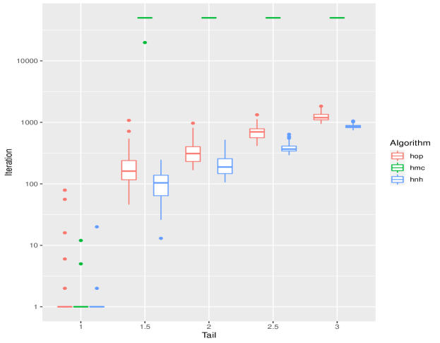
Figure 8: Iteration number at which Hop, HMC, and Hug and Hop converged to the main mass of the target  (13) with $a=4$. The x-axis denotes the starting multiplier $\gamma$.

Appendix H Example targets

Firstly, consider an equal mixture of two $\mathsf{N}\left(\mu_{i},\Sigma_{i}\right)$ distributions, then $\mathbb{E}\left[{X}\right]=\frac{1}{2}(\mu_{1}+\mu_{2})$ and

$$\mathsf{Cov}\left[{X}\right] =\frac{1}{2}\Sigma_{1}+\frac{1}{2}\Sigma_{2}+\frac{1}{4}(\mu_{1}-\mu_{2})(\mu_{1}-\mu_{2})^{\top}.$$ (31)

H.1 Banana

The Banana target is parameterised by $\lambda\in(0,1)$, its bananacity. The two components $(x_{1},x_{2})$ satisfy:

$$X_{1}\sim\mathsf{N}(0,1),\qquad X_{2}|x_{1}\sim\mathsf{N}(\lambda(x_{1}^{2}-1),1-\lambda^{2}).$$

Values of $\lambda$ closer to one make the banana bendier, whilst at $\lambda=0$ the target degenerates to a $\mathsf{N}\left(0,I\right)$. The log-target for this model is thus:

$$\log\pi(x)=-\frac{x_{1}^{2}}{2}-\frac{(x_{2}-\lambda(x_{1}^{2}-1))^{2}}{2(1-\lambda^{2})}.$$

H.2 Bimodal

The Bimodal is an equal mixture of two bivariate Normal distributions:

$$X\sim\frac{1}{2}\mathsf{N}(-\mu,\Sigma)+\frac{1}{2}\mathsf{N}(\mu,\Sigma).$$

with $\mu=\sqrt{\lambda}\bm{1}$ and $\Sigma=(1-\lambda)I$. Thus, $\mathbb{E}\left[{X}\right]=0$ and, by (31), $\mathsf{Cov}\left[{X}\right]=\Sigma+\mu\mu^{\top}=(1-\lambda)I+\lambda\bm{1}\bm{1}^{\top}$. For the main experiments, the results of which are summarised in Figure 3, we set $\lambda=0.95$.

For the extreme experiment at the end of Section 3 we set $\lambda=0.9$ and an overall scale for component $i$ of $1+9(d-i)/(d-1)$. We chose these values so that the algorithms with no preconditioning were able to travel between the modes, but that such movement happened relatively rarely.

Over five replicate experiments, each of $2\times 10^{5}$ iterations, the best-performing NUTS algorithm used $\epsilon=1.95$, which led to an acceptance rate of $84\%$, a mean CPU time of $134\%$ of that of HMC and $(17,14,10,23,16)$ mode flips (mean$=16$). The best performing HMC algorithm used $T=20$ and $L=15$, which led to an acceptance rate of $83\%$ and $(31,28,37,34,36)$ mode flips (mean$=33.2$). The best performing Hug and Hop algorithm used $T=30$, $B=16$, $\lambda=5$ and $\kappa=1$, which led to acceptance rates of $\alpha_{hug}=63\%$ and $\alpha_{hop}=23\%$, a mean CPU time of $149\%$ of that of HMC and $(75,83,67,63,77)$ mode flips (mean$=73$).

Figure 9 provides trace plots for each of the three algorithms from the final replicate for each experiment, as well as the true density along the line between the two modes. The scale of $x_{25}$, which is $1$, restricts the sizes of the steps that lead to reasonable acceptance rates; the size of the gap between the modes should be viewed relative to this. The algorithms were tuned so to maximise mode hopping, nonetheless, when comparing the minimum effective sample size over the $23$ unimodal components, that of Hug and Hop was $163\%$ of that of HMC, indicating that it is slightly more efficient in these terms, too.

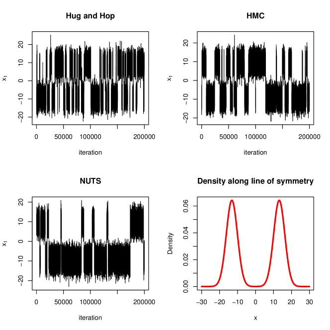
Figure 9: Trace plots for $x_{1}$ from Hug and Hop, HMC and NUTS for the extreme bimodal target, and the (both marginal and conditional) density along the line of symmetry between the modes.

H.3 PlusPrism

The PlusPrism is an equal mixture of two centred bi-variate Normal distributions with covariance matrices $\Sigma_{1}=\mathsf{diag}(1+\lambda,1-\lambda)$ and $\Sigma_{2}=\mathsf{diag}(1-\lambda,1+\lambda)$. The overall mean is at $\bm{0}$, while the covariance is given by $\mathsf{Cov}\left[{X}\right]=(\Sigma_{1}+\Sigma_{2})/2=I$. We set $\lambda=0.95$.

This target has mass spread in a “+” shape along the $x$ and $y$ axis with a mode at (0,0). In three or more dimensions, this two-dimensional plus is projected along the other dimensions creating a prism.

Appendix I Statistical models

I.1 Cauchit regression

To simplify the formulae, we redefine the response to be $Y_{i}\in\{-1,1\}$ rather than $Y_{i}\in\{0,1\}$. The inverse link function is $g^{-1}(x)=1/2+\arctan(x)/\pi$, where, here only, $\pi$ is the number $3.14\dots$. Now, $g^{-1}(-x)=1-g^{-1}(x)$, and writing $\eta_{i}=x_{i}^{\top}\beta$,

$$\ell(\beta) =-\frac{\tau}{2}\left|\left|{\beta}\right|\right|^{2}+\sum_{i}\log\left(1/2+\arctan(y_{i}\eta_{i})/\pi\right),$$

$$\frac{\partial\ell}{\partial\beta_{j}} =-\tau\beta_{j}+\sum_{i}\frac{y_{i}x_{ij}}{(1+\eta_{i}^{2})\left(\pi/2+\arctan(y_{i}\eta_{i})\right)}.$$

Figure 10 shows the effect of varying the Hop tuning parameters on the Hop acceptance rate and efficiency of exploration of the 100-dimensional Cauchit-regression posterior. The Hug tuning parameters were set to values that explored the posterior adequately, but not optimally; very similar patterns were found with other settings for the Hug parameters where mixing was at least adequate.

The left-hand plot shows that for small to moderate values of $\lambda$, the acceptance rate is close to the theoretical value, but as $\lambda$ increases towards and then beyond $d^{1/2}=10$ the acceptance probability drops monotonically towards zero. The right-hand plot shows that in this example, whatever the setting of $\kappa$, the optimal choice of $\lambda$ is achieved when the acceptance rate is around a third to a half of the asymptotic rate for that $\kappa$ value; i.e., when the asymptotics have started to break down but have not completely broken down.

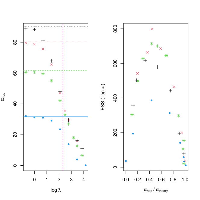
Figure 10: Hug and Hop applied to a 100-dimensional Cauchit-regression posterior with Hug parameters fixed at $(T=0.32,B=4)$. Hop parameters were varied, with and $\lambda\in\{1/2,1,2,4,8,12,16,32,48\}$ and $\kappa\in\{1/4,1/2,1,2\}$. Points and lines are coloured according to $\kappa$: black $+$ and dot-dashed-line ($\kappa=1/4$); red $\times$ and dotted line ($\kappa=1/2$); green $*$ and dashed line ($\kappa=1$); blue $\bullet$ and solid line ($\kappa=2$). The left plot shows the acceptance rate as a function of $\lambda$, with horizontal lines marking the theoretical acceptance rate, the vertical magenta line corresponds to $\lambda=d^{1/2}=10$; the right plot shows the effective sample size of $\log\pi$ as a function of the ratio of the observed acceptance rate to the asymptotic acceptance rate.

I.2 Rasch model

As with the Cauchit regression we redefine the response to be $Y_{ij}\in\{-1,1\}$ and let $z_{ij}=y_{ij}(\eta_{i}-\beta_{j})$. Then:

$$\ell(\beta,\eta|y) =\sum_{i,j=1}^{M,N}\log\Phi(z_{ij})-\frac{\tau}{2}\sum_{i=1}^{M}\eta_{i}^{2}-\frac{\tau}{2}\sum_{j=1}^{M}\beta_{j}^{2},$$

$$\frac{\partial\ell}{\partial\eta_{k}} =\sum_{j=1}^{N}y_{kj}\frac{\phi(z_{kj})}{\Phi(z_{kj})}-\tau\eta_{k},$$

$$\frac{\partial\ell}{\partial\beta_{k}} =\sum_{i=1}^{M}-y_{ik}\frac{\phi(z_{ik})}{\Phi(z_{ik})}-\tau\beta_{k}.$$

I.3 Stochastic volatility model

Let $t=0,\dots,T-1$ be $T$ index equally spaced moments in time and consider the following model:

$$z_{t} \sim\mathsf{N}(0,1)~{}~{}~{}\mbox{i.i.d},$$

$$x_{0} =\frac{z_{0}}{\phi},$$

$$x_{t} =\rho x_{t-1}+z_{t},$$

$$y_{t} \sim\mathsf{N}\left(0,\frac{\exp(2x_{t})}{\tau}\right),$$

with $\phi=\sqrt{1-\rho^{2}}$ and prior distributions of $\tau\sim\mathsf{Gamma}(21,5)$ and $(1+\rho)/2\sim\mathsf{Beta}(20,2)$.

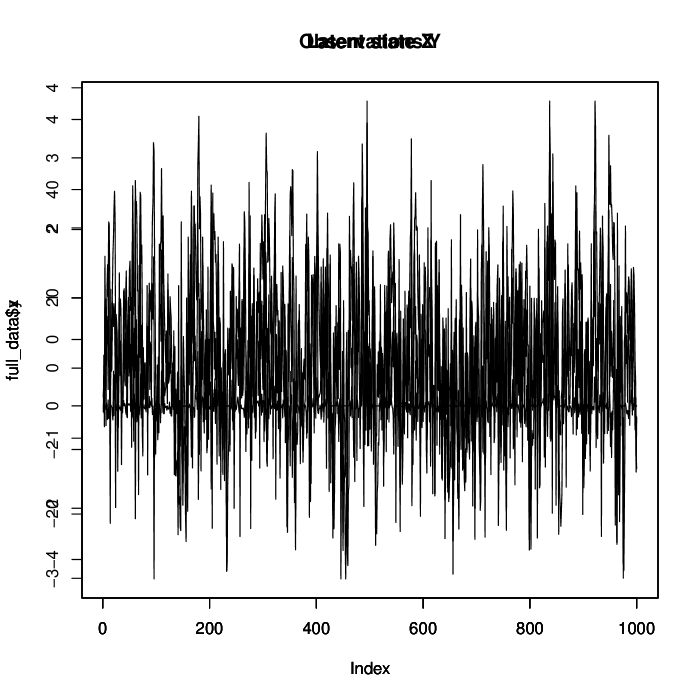
Figure 11: Simulated data for the Stochastic volatility data study.

The data simulated from this model and used in Section 4.3 are shown in Figure 11. To perform inference, we consider the posterior distribution on $z$ and the parameters $(\alpha,\beta)$, which map $(\tau,\rho)$ to the real line via the equations:

$$\alpha=-\frac{1}{2}\log(\tau),\quad\beta=\frac{1}{2}\log\left(\frac{1+\rho}{1-\rho}\right)$$

with inverses:

$$\tau=\exp(-2\alpha),\quad\rho=\frac{\exp(2\beta)-1}{\exp(2\beta)+1}=\tanh\beta.$$

Up to additive constants, the prior log-densities for $\tau$ and $\rho$ are:

$$\log f_{\tau}(\tau) =20\log(\tau)-5\tau$$

$$\log f_{\rho}(\rho) =19\log(1+\rho)+\log(1-\rho)=20\log(1+\rho)-\log\left(\frac{1+\rho}{1-\rho}\right).$$

Thus, ignoring additive constants, the log-prior for $\alpha$ is:

$$\log f_{\alpha}(\alpha) =\log f_{\tau}(\tau(\alpha))+\log\left|{\frac{\operatorname{\mathsf{d}}\!{\tau}}{\operatorname{\mathsf{d}}\!{\alpha}}}\right|=-40\alpha-5\exp(-2\alpha)-2\alpha$$

$$=-42\alpha-5\exp(-2\alpha).$$

To obtain the log prior for $\beta$, $\log f_{\beta}(\beta)$, first note that:

$$\left|{\frac{\operatorname{\mathsf{d}}\!{\rho}}{\operatorname{\mathsf{d}}\!{\beta}}}\right|=\mathsf{sech}^{2}\beta=\frac{4\exp(-2\beta)}{(1+\exp(-2\beta))^{2}},$$

and

$$\log(1+\rho)=\log\left(\frac{\exp(2\beta)}{\exp(2\beta)+1}\right)=-\log\left\{1+\exp(-2\beta)\right\}.$$

Thus, ignoring additive constants,

$$\log f_{\beta}(\beta) =\log f_{\nu}(\rho(\beta))+\log\left|{\frac{\operatorname{\mathsf{d}}\!{\rho}}{\operatorname{\mathsf{d}}\!{\beta}}}\right|$$

$$=-20\log(1+\exp(-2\beta))-2\beta-2\beta-2\log\left\{1+\exp(-2\beta)\right\}$$

$$=-22\log\{1+\exp(-2\beta)\}-4\beta.$$

We now derive the log-posterior distribution in terms of $\alpha$ and $\beta$. Since $\phi=\sqrt{1-\rho^{2}}=\mathsf{sech}{\beta}$, the model for the data is now:

$$x_{0} =z_{0}\cosh\beta,$$

$$x_{t} =\tanh(\beta)x_{t-1}+z_{t},$$

$$y_{t} \sim\mathsf{N}\left(0,\exp(2\alpha+2x_{t})\right).$$

Ignoring additive constants, the log-likelihood is

$$\ell(z,y;\alpha,\beta) =-\frac{1}{2}\sum_{t=0}^{T-1}z_{t}^{2}-\frac{1}{2}\sum_{t=0}^{T-1}\left\{2\alpha+2x_{t}+\left(\exp(2\alpha+2x_{t})\right)^{-1}y_{t}^{2}\right\}.$$

$$=-T\alpha-\frac{1}{2}\sum_{t=0}^{T-1}z_{t}^{2}+2x_{t}+\exp(-2\alpha-2x_{t})y_{t}^{2}.$$

Setting $w_{t}=\exp(-2x_{t}-2\alpha)y_{t}^{2}$,

$$\log\pi(z,\alpha,\beta|y)=-42\alpha-5e^{-2\alpha}-22\log\left(1+e^{-2\beta}\right)-4\beta-T\alpha-\sum_{t=0}^{T}x_{t}-\frac{1}{2}\sum_{t=0}^{T-1}\left(w_{t}+z_{t}^{2}\right).$$

I.4 Gradients

We have $\partial\log f_{\alpha}/\partial\alpha=-42+10\exp(-2\alpha)$ and since $x_{t}$ does not depend on $\alpha$, $\partial\ell/\partial\alpha=-T+\exp(-2\alpha)\sum_{t=0}^{T-1}\exp(-2x_{t})y_{t}^{2}$. Thus

$$\frac{\partial\log\pi}{\partial\alpha}=-42-T+10\exp(-2\alpha)+\exp(-2\alpha)\sum_{t=0}^{T-1}\exp(-2x_{t})y_{t}^{2}.$$

Now

$$\frac{\partial\log f_{\beta}}{\partial\beta}=-22\left(\frac{-2\exp(-2\beta)}{1+\exp(-2\beta)}\right)-4=\frac{44}{1+\exp(2\beta)}-4.$$

Also

$$\frac{\partial\ell}{\partial\beta}=-\frac{1}{2}\sum_{t=0}^{T-1}2\frac{\partial x_{t}}{\partial\beta}-2\frac{\partial x_{t}}{\partial\beta}\exp(-2\alpha-2x_{t})y_{t}^{2}$$

$$=\sum_{t=0}^{T-1}\left\{\exp(-2\alpha-2x_{t})y_{t}^{2}-1\right\}\frac{\partial x_{t}}{\partial\beta}.$$

So

$$\frac{\partial\log\pi}{\partial\beta}=\frac{44}{1+\exp(2\beta)}-4+\sum_{t=0}^{T-1}\left\{\exp(-2\alpha-2x_{t})y_{t}^{2}-1\right\}\frac{\partial x_{t}}{\partial\beta}.$$

At $t=0$:

$$\frac{\partial{x_{0}}}{\partial{\beta}} =\frac{\partial{}}{\partial{\beta}}\left(z_{0}\cosh\beta\right)=z_{0}\sinh\beta=\tanh(\beta)x_{0}$$

For $t=1\to T-1$, $x_{t}=\tanh(\beta)x_{t-1}+z_{t}$, so

$$\frac{\partial{x_{t}}}{\partial{\beta}} =\tanh(\beta)\frac{\partial{x_{t-1}}}{\partial{\beta}}+\mathsf{sech}^{2}(\beta)x_{t-1}$$

We compute these terms recursively.

Finally,

$$\frac{\partial\log\pi}{\partial z_{s}} =\frac{\partial\ell}{\partial z_{s}}=-\sum_{t=0}^{T-1}z_{t}\mathbb{I}\left({t=s}\right)+\frac{\partial x_{t}}{\partial z_{s}}-2\frac{\partial x_{t}}{\partial z_{s}}\exp(-2\alpha-2x_{t})y_{t}^{2}$$

$$=-z_{s}+\sum_{t=0}^{T-1}\left\{\exp(-2\alpha-2x_{t})y_{t}^{2}-1\right\}\frac{\partial x_{t}}{\partial z_{s}}.$$

When $t=0$ we have:

$$\frac{\partial{x_{0}}}{\partial{z_{s}}}=\cosh(\beta)\frac{\partial{z_{0}}}{\partial{z_{s}}}=\cosh(\beta)\mathbb{I}\left({s=0}\right).$$

For $t=1\to T-1$:

$$\frac{\partial{x_{t}}}{\partial{z_{s}}}=\frac{\partial{}}{\partial{z_{s}}}\left\{\tanh(\beta)x_{t-1}+z_{t}\right\}=\tanh(\beta)\frac{\partial{x_{t-1}}}{\partial{z_{s}}}+\mathbb{I}\left({s=t}\right)$$

The solution to these recursions is:

$$\frac{\partial{x_{t}}}{\partial{z_{s}}}=\tanh^{t-s}\beta\cosh^{\mathbb{I}\left({s=0}\right)}\beta\mathbb{I}\left({s\leq t}\right).$$

References

- Besag, (1994) Besag, J. (1994). In discussion of ‘Representations of knowledge in complex systems’ by U. Grenander and M. Miller. J. Roy. Stat. Soc. Ser. B, 56:591–592.
- Bierkens, (2015) Bierkens, J. (2015). Non-reversible Metropolis-Hastings. Statistics and Computing, 26(6):1213–1228.
- Bouchard-Côté et al., (2018) Bouchard-Côté, A., Vollmer, S. J., and Doucet, A. (2018). The bouncy particle sampler: A nonreversible rejection-free Markov chain Monte Carlo method. Journal of the American Statistical Association, 113(522):855–867.
- Brooks et al., (2011) Brooks, S., Gelman, A., Jones, G., and Meng, X.-L. (2011). Handbook of Markov chain Monte Carlo. CRC press.
- Diaconis et al., (2000) Diaconis, P., Holmes, S., and Neal, R. M. (2000). Analysis of a nonreversible Markov chain sampler. The Annals of Applied Probability, 10(3):726–752.
- Fearnhead et al., (2018) Fearnhead, P., Bierkens, J., Pollock, M., and Roberts, G. O. (2018). Piecewise deterministic Markov processes for continuous-time Monte Carlo. Statistical Science, 33(3):386–412.
- Girolami and Calderhead, (2011) Girolami, M. and Calderhead, B. (2011). Riemann manifold Langevin and Hamiltonian Monte Carlo methods. Journal of the Royal Statistical Society: Series B (Statistical Methodology), 73(2):123–214.
- Hastings, (1970) Hastings, W. K. (1970). Monte carlo sampling methods using Markov chains and their applications. Biometrika, 57(1):97–109.
- Hoffman and Gelman, (2014) Hoffman, M. D. and Gelman, A. (2014). The No-U-Turn sampler: adaptively setting path lengths in hamiltonian Monte Carlo. Journal of Machine Learning Research, 15(1):1593–1623.
- Koenker and Yoon, (2009) Koenker, R. and Yoon, J. (2009). Parametric links for binary choice models: A Fisherian – Bayesian colloquy. Journal of Econometrics, 152(2):120–130.
- Leimkuhler et al., (2004) Leimkuhler, B., Reich, S., and Press, C. U. (2004). Simulating Hamiltonian Dynamics. Cambridge Monographs on Applied and Computational Mathematics. Cambridge University Press.
- Livingstone et al., (2019) Livingstone, S., Betancourt, M., Byrne, S., and Girolami, M. (2019). On the geometric ergodicity of Hamiltonian Monte Carlo. Bernoulli, 25(4A):3109–3138.
- Ma et al., (2018) Ma, Y.-A., Fox, E. B., Chen, T., and Wu, L. (2018). Irreversible samplers from jump and continuous Markov processes. Statistics and Computing.
- Mallik and Jones, (2017) Mallik, A. and Jones, G. L. (2017). Directional Metropolis-Hastings. arXiv preprint arXiv:1710.09759.
- Mengersen and Tweedie, (1996) Mengersen, K. L. and Tweedie, R. L. (1996). Rates of convergence of the Hastings and Metropolis algorithms. Ann. Statist., 24(1):101–121.
- Neal, (1998) Neal, R. M. (1998). Suppressing random walks in Markov Chain Monte Carlo using ordered overrelaxation. In Learning in Graphical Models, pages 205–228. Springer Netherlands.
- Neal, (2011) Neal, R. M. (2011). MCMC using Hamiltonian dynamics. In Brooks, S., Gelman, A., Jones, G., and Meng, X.-L., editors, Handbook of Markov chain Monte Carlo, chapter 5, pages 113–162. CRC press.
- Pakman et al., (2017) Pakman, A., Gilboa, D., Carlson, D., and Paninski, L. (2017). Stochastic bouncy particle sampler. In Precup, D. and Teh, Y. W., editors, Proceedings of the 34th International Conference on Machine Learning, volume 70 of Proceedings of Machine Learning Research, pages 2741–2750, International Convention Centre, Sydney, Australia. PMLR.
- Peters and de With, (2012) Peters, E. A. J. F. and de With, G. (2012). Rejection-free monte carlo sampling for general potentials. Phys. Rev. E, 85:026703.
- Rasch, (1980) Rasch, G. (1980). Probabilistic models for some intelligence and attainment tests. University of Chicago Press, Chicago, expanded ed. edition.
- Roberts et al., (1997) Roberts, G. O., Gelman, A., Gilks, W. R., et al. (1997). Weak convergence and optimal scaling of random walk Metropolis algorithms. The annals of applied probability, 7(1):110–120.
- Roberts and Rosenthal, (1998) Roberts, G. O. and Rosenthal, J. S. (1998). Optimal scaling of discrete approximations to Langevin diffusions. Journal of the Royal Statistical Society: Series B (Statistical Methodology), 60(1):255–268.
- Roberts and Rosenthal, (2001) Roberts, G. O. and Rosenthal, J. S. (2001). Optimal scaling for various Metropolis-hastings algorithms. Statist. Sci., 16(4):351–367.
- Roberts and Rosenthal, (2004) Roberts, G. O. and Rosenthal, J. S. (2004). General state space Markov chains and MCMC algorithms. Probab. Surveys, 1:20–71.
- (25) Roberts, G. O. and Tweedie, R. L. (1996a). Exponential convergence of Langevin distributions and their discrete approximations. Bernoulli, 2(4):341–363.
- (26) Roberts, G. O. and Tweedie, R. L. (1996b). Geometric convergence and central limit theorems for multidimensional Hastings and Metropolis algorithms. Biometrika, 83(1):95–110.
- Sejdinovic et al., (2014) Sejdinovic, D., Strathmann, H., Garcia, M. L., Andrieu, C., and Gretton, A. (2014). Kernel adaptive metropolis-hastings. In International Conference on Machine Learning, pages 1665–1673.
- Sherlock et al., (2010) Sherlock, C., Fearnhead, P., and Roberts, G. O. (2010). The random walk Metropolis: Linking theory and practice through a case study. Statist. Sci., 25(2):172–190.
- Sherlock and Thiery, (2021) Sherlock, C. and Thiery, A. H. (2021). A Discrete Bouncy Particle Sampler. Biometrika. asab013.
- Vanetti et al., (2017) Vanetti, P., Bouchard-Côté, A., Deligiannidis, G., and Doucet, A. (2017). Piecewise deterministic Markov chain Monte Carlo. arXiv preprint arXiv:1707.05296.
- Wu and Robert, (2020) Wu, C. and Robert, C. P. (2020). The coordinate sampler: A non-reversible Gibbs-like MCMC sampler. Statistics and Computing, 30:721–730.