Level-Planar Drawings with Few Slopes

Abstract

We introduce and study level-planar straight-line drawings with a fixed number $\lambda$ of slopes. For proper level graphs, we give an $O(n\log^{2}n/\log\log n)$-time algorithm that either finds such a drawing or determines that no such drawing exists. Moreover, we consider the partial drawing extension problem, where we seek to extend an immutable drawing of a subgraph to a drawing of the whole graph, and the simultaneous drawing problem, which asks about the existence of drawings of two graphs whose restrictions to their shared subgraph coincide. We present $O(n^{4/3}\log n)$-time and $O(\lambda n^{10/3}\log n)$-time algorithms for these respective problems on proper level-planar graphs.

We complement these positive results by showing that testing whether non-proper level graphs admit level-planar drawings with $\lambda$ slopes is NP-hard even in restricted cases.

1 Introduction

Directed graphs explaining hierarchy naturally appear in multiple industrial and academic applications. Some examples include PERT diagrams, UML component diagrams, text edition networks [1], text variant graphs [20], philogenetic and neural networks. In these, and many other applications, it is essential to visualize the implied directed graph so that the viewer can perceive the hierarchical structure it contains. By far the most popular way to achieve this is to apply the Sugyiama framework – a generic network visualization algorithm that results in a drawing where each vertex lies on a horizontal line, called layer, and each edge is directed from a lower layer to a higher layer [15].

The Sugyiama framework consists of several steps: elimination of directed cycles in the initial graph, assignement of vertices to layers, vertex ordering and coordinate assignement. During each of these steps several criteria are optimized, by leading to more readable visualizations, see e.g. [15]. In this paper we concentrate on the last step of the framework, namely coordinate assignment. Thus, the subject of our study are level graphs defined as follows. Let $G=(V,E)$ be a directed graph. A $k$-level assignment of $G$ is a function $\ell:V\to\{1,2,\dots,k\}$ that assigns each vertex of $G$ to one of $k$ levels. We refer to $G$ together with $\ell$ as to a ($k$-)level graph. The length of an edge $(u,v)$ is defined as $\ell(v)-\ell(u)$. We say that $G$ is proper if all edges have length one. The level graph shown in Fig. 1 (a) is proper, whereas the one shown in (b) is not. For a non-proper level graph $G$ there exists a proper subdivision obtained by subdividing all edges with length greater than one which result in a proper graph.

A level drawing $\Gamma$ of a level graph $G$ maps each vertex $v\in V$ to a point on the horizontal line with $y$-coordinate $\ell(v)$ and a real $x$-coordinate $\Gamma(v)$, and each edge to a $y$-monotone curve between its endpoints. A level drawing is called level-planar if no two edges intersect except in common endpoints. It is straight-line if the edges are straight lines. A level drawing of a proper (subdivision of a) level graph $G$ induces a total left-to-right order on the vertices of a level. We say that two drawings are equivalent if they induce the same order on every level. An equivalence class of this equivalence relation is an embedding of $G$. We refer to $G$ together with an embedding to as embedded level graph $\mathcal{G}$. The third step of Sugyiama framework, vertex ordering, results in an embedded level graph.

The general goal of the coordinate assignment step is to produce a final visualization while further improving its readability. The criteria of readability that have been considered in the literature for this step include straightness and verticality of the edges [15]. Here we study the problem of coordinate assignment step with bounded number of slopes. The slope of an edge $(u,v)$ in $\Gamma$ is defined as $(\Gamma(v)-\Gamma(u))/(\ell(v)-\ell(u))$. For proper level graphs this simplifies to $\Gamma(v)-\Gamma(u)$. We restrict our study to drawings in which all slopes are non-negative; such drawings can be transformed into drawings with negative slopes by shearing; see Fig. 1.

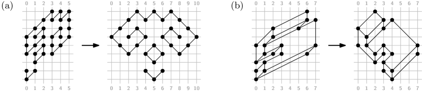
Figure 1: Shearing drawings to change the slopes. In (a), the left drawing with slopes $0$ and $1$ is transformed into the right orthogonal drawing, i.e., one with slopes $-1$ and $1$. In (b), the left drawing with slopes $0,1$ and $2$ is transformed into a drawing with slopes $-1,0$ and $1$.

A level drawing $\Gamma$ is a $\lambda$-slope drawing if all slopes in $\Gamma$ appear in the set $\{0,1,\dots,\lambda-1\}$. We study embedding-preserving straight-line level-planar $\lambda$-slope drawings, or $\lambda$-drawings for short and refer to the problem of finding these drawings as $\lambda$-Drawability . Since the possible edge slopes in a $\lambda$-drawing are integers all vertices lie on the integer grid.

Related Work.

The number of slopes used for the edges in a graph drawing can be seen as an indication of the simplicity of the drawing. For instance, the measure edge orthogonality, which specifies how close a drawing is to an orthogonal drawing, where edges are polylines consisting of horizontal and vertical segments only, has been proposed as a measure of aesthetic quality of a graph drawing [33]. In a similar spirit, Kindermann et al. studied the effect reducing the segment complexity on the aesthetics preference of graph drawings and observed that in some cases people prefer drawings using lower segment complexity [23]. More generally, the use of few slopes for a graph drawing may contribute to the formation of “Prägnanz” (“good figure” in German) of the visualization, that accordingly to the Gestalt law of Prägnanz, or law of simplicity, contributes to the perceived quality of the visualizations. This is design principle often guides the visualization of metro maps. See [30] for a survey of the existing approaches, most of which generate octilinear layouts of metro maps, and [29] for a recent model for drawing more general $k$-linear metro maps.

Level-planar drawing with few slopes have not been considered in the literature but drawings of undirected graphs with few slopes have been extensively studied. The (planar) slope number of a (planar) graph $G$ is the smallest number $s$ so that $G$ has a (planar) straight-line drawing with edges of at most $s$ distinct slopes. Special attention has been given to proving bounds on the (planar) slope number of undirected graph classes [4, 9, 10, 11, 13, 22, 21, 24, 25, 31]. Determining the planar slope number is hard in the existential theory of reals [17].

Several graph visualization problems have been considered in the partial and simultaneous settings. In the partial drawing extension problem, one is presented with a graph and an immutable drawing of some subgraph thereof. The task is to determine whether the given drawing of the subgraph can be completed to a drawing of the entire graph. The problem has been studied for the planar setting [26, 32] and also the level-planar setting [7]. In the simultaneous drawing problem, one is presented with two graphs that may share some subgraph. The task is to draw both graphs so that the restrictions of both drawings to the shared subgraph are identical. We refer the reader to [5] for an older literature overview. The problem has been considered for orthogonal drawings [2] and level-planar drawings [3]. Up to our knowledge, neither partial nor simultaneous drawings have been considered in the restricted slope setting.

Contribution.

We introduce and study the $\lambda$-Drawability problem. To solve this problem for proper level graphs, we introduce two models. In Section 3 we describe the first model, which uses a classic integer-circulation-based approach. This model allows us to solve the $\lambda$-Drawability in $O(n\log^{3}n)$ time and obtain a $\lambda$-drawing within the same running time if one exists. In Section 4, we describe the second distance-based model. It uses the duality between flows in the primal graph and distances in the dual graph and allows us to solve the $\lambda$-Drawability in $O(n\log^{2}n/\log\log n)$ time. We also address the partial and simultaneous settings. The classic integer-circulation-based approach can be used to extend connected partial $\lambda$-drawings in $O(n\log^{3}n)$ time. In Section 5, we build on the distance-based model to extend not-necessarily-connected partial $\lambda$-drawings in $O(n^{4/3}\log n)$ time, and to obtain simultaneous $\lambda$-drawings in $O(\lambda n^{10/3}\log n)$ time if they exist. We finish with some concluding remarks in Section 6 and refer to Appendix 0.A for a proof that 2-Drawability is NP-hard even for biconnected graphs where all edges have length one or two.

2 Preliminaries

Let $\Gamma$ be a level-planar drawing of an embedded level-planar graph $\cal G$. The width of $\Gamma$ is defined as $\max_{v\in V}\Gamma(v)-\min_{v\in V}\Gamma(v)$. An integer $\bar{x}$ is a gap in $\Gamma$ if it is $\Gamma(v)\neq\bar{x}$ for all $v\in V$, $\Gamma(v_{1})<\bar{x}$ and $\Gamma(v_{2})>\bar{x}$ for some $v_{1},v_{2}\in V$, and $\Gamma(u)<\bar{x}<\Gamma(v)$ for no edge $(u,v)\in E$. A drawing $\Gamma$ is compact if it has no gap. Note that a $\lambda$-drawing of a connected level-planar graph is inherently compact. While in a $\lambda$-drawing of a non-connected level-planar graph every gap can be eliminated by a shift. The fact that we only need to consider compact $\lambda$-drawings helps us to limit their width. Thus, any compact $\lambda$-drawing has a width of at most $(\lambda-1)(n-1)$.

Let $u$ and $v$ be two vertices on the same level $i$. With $[u,v]_{\mathcal{G}}$ (or $[u,v]$ when $\mathcal{G}$ is clear from the context) we denote the set of vertices that contains $u,v$ and all vertices in between $u$ and $v$ on level $i$ in $\mathcal{G}$. We say that two vertices $u$ and $v$ are consecutive in $\mathcal{G}$ when $[u,v]=\{u,v\}$. Two edges $e=(u,w),e^{\prime}=(v,x)$ are consecutive in $\mathcal{G}$ when the only edges with one endpoint in $[u,v]_{\mathcal{G}}$ and the other endpoint in $[w,x]_{\mathcal{G}}$ are $e$ and $e^{\prime}$.

A flow network $F=(N,A)$ consists of a set of nodes $N$ connected by a set of directed arcs $A$. Each arc has a demand specified by a function $d:A\to\mathbb{N}_{0}$ and a capacity specified by a function $c:A\to\mathbb{N}\cup\{\infty\}$ where $\infty$ encodes unlimited capacity. A circulation in $F$ is a function $\varphi:A\to\mathbb{N}_{0}$ that assigns an integral flow to each arc of $F$ and satisifies the two following conditions. First, the circulation has to respect the demands and capacities of the arcs, i.e., for each arc $a\in A$ it is $d(a)\leq\varphi(a)\leq c(a)$. Second, the circulation has to respect flow conservation, i.e., for each node $v\in N$ it is $\sum_{(u,v)\in A}\varphi(u,v)=\sum_{(v,u)\in A}\varphi(v,u)$. Depending on the flow network no circulation may exist.

3 Flow Model

In this section, we model the $\lambda$-Drawability as a problem of finding a circulation in a flow network. Let $\mathcal{G}$ be an embedded proper $k$-level graph together with a level-planar drawing $\Gamma$. As a first step, we add two directed paths $p_{\operatorname{left}}$ and $p_{\operatorname{right}}$ that consist of one vertex on each level from 1 to $k$ to $\mathcal{G}$. Insert $p_{\operatorname{left}}$ and $p_{\operatorname{right}}$ into $\Gamma$ to the left and right of all other vertices as the left and right boundary, respectively. See Fig. 2 (a) and (c).

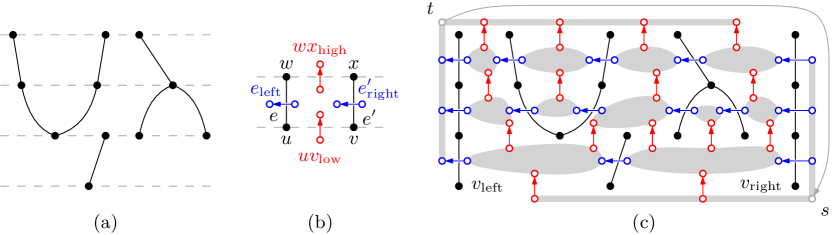
Figure 2: (a) An embedded level graph $\mathcal{G}$. (b) The definition of the arcs of the flow network. (c) The graph $\mathcal{G}$ together with the paths $p_{\operatorname{left}}$ and $p_{\operatorname{right}}$ in black. The resulting flow network $F_{\mathcal{G}}^{\lambda}$ (c) consists of the blue slope arcs and the red space arcs, its nodes are formed by merging the nodes in the gray areas. The red space arcs have a demand of $1$ and a capacity of $(\lambda-1)(n-1)$ and the blue slope arcs have a demand of zero and a capacity of $\lambda-1$.

From now on, we assume that $\mathcal{G}$ and $\Gamma$ contain the left and right boundary.

The flow network $F_{\mathcal{G}}^{\lambda}$ consists of nodes and arcs and is similar to a directed dual of $\mathcal{G}$ with the difference that it takes the levels of $\mathcal{G}$ into account. In particular, for every edge $e$ of $\mathcal{G}$, $F_{\mathcal{G}}^{\lambda}$ contains two nodes $e_{\operatorname{left}}$ and $e_{\operatorname{right}}$, in the left and the right faces incident to $e$, and a dual slope arc $e^{\star}=(e_{\operatorname{right}},e_{\operatorname{left}})$ with demand $0$ and capacity $\lambda-1$; see the blue arcs in Fig. 2 (b) and (c). The flow across $e^{\star}$ determines the slope of $e$. Additionally, for every pair of consecutive vertices $u,v$ we add two nodes $[u,v]_{\operatorname{low}}$ and $[u,v]_{\operatorname{high}}$ to $F_{\mathcal{G}}^{\lambda}$ and connect them by a space arc $[u,v]^{\star}$; see the red arcs in Fig. 2 (b) and (c). The flow across $[u,v]^{\star}$ determines the space between $u$ and $v$. The space between $u$ and $v$ needs to be at least one to prevent $u$ and $v$ from colliding and can be at most $(\lambda-1)(n-1)$ due to the restriction to compact drawings. So, assign to $[u,v]^{\star}$ a demand of one and a capacity of $(\lambda-1)(n-1)$. To obtain the final flow network we merge certain nodes. Let $e=(u,w)$ and $e^{\prime}=(v,x)$ be consecutive edges. Merge the nodes $e_{\operatorname{right}},e^{\prime}_{\operatorname{left}}$, the nodes $\{\{u^{\prime},v^{\prime}\}_{\operatorname{high}}:\forall u^{\prime},v^{\prime}\textrm{~{}consecutive in~{}}[u,v]\}$ and the nodes $\{\{w^{\prime},x^{\prime}\}_{\operatorname{low}}:\forall w^{\prime},x^{\prime}\textrm{~{}consecutive in~{}}[w,x]\}$ into a single node. Next, merge all remaining source and sink nodes into one source node $s$ and one sink node $t$, respectively. See Fig. 2 (c), where the gray areas touch nodes that are merged into a single node. Finally, insert an arc from $t$ to $s$ with unlimited capacity.

The network $F_{\mathcal{G}}^{\lambda}$ is designed in such a way that the circulations in $F_{\mathcal{G}}^{\lambda}$ correspond bijectively to the $\lambda$-drawings of $\mathcal{G}$. Let $\Gamma$ be a drawing of $\mathcal{G}$ and let $x$ be the function that assigns to each vertex of $\mathcal{G}$ its $x$-coordinate in $\Gamma$. We define a dual circulation $x^{\star}$ as follows. Recall that every arc $a$ of $F_{\mathcal{G}}^{\lambda}$ is either dual to an edge of $\mathcal{G}$ or to two consecutive vertices in $\mathcal{G}$. Hence, the left and right incident faces $f_{\operatorname{left}}$ and $f_{\operatorname{right}}$ of $a$ in $F_{\mathcal{G}}^{\lambda}$ contain vertices of $\mathcal{G}$. Define the circulation $x^{\star}$ by setting $x^{\star}(a):=x(f_{\operatorname{right}})-x(f_{\operatorname{left}})$. We remark the following, although we defer the proof to the next section.

Lemma 1

Let $\mathcal{G}$ be an embedded proper level-planar graph together with a $\lambda$-drawing $\Gamma$. The dual $x^{\star}$ of the function $x$ that assigns to each vertex of $\mathcal{G}$ its $x$-coordinate in $\Gamma$ is a circulation in $F_{\mathcal{G}}^{\lambda}$.

In the reverse direction, given a circulation $\varphi$ in $F_{\mathcal{G}}^{\lambda}$ we define a dual function $\varphi^{\star}$ that, when interpeted as assigning an $x$-coordinate to the vertices of $\mathcal{G}$, defines a $\lambda$-drawing of $G$. Refer to the level-1-vertex $p_{\operatorname{right}}$ as $v_{\operatorname{right}}$. Start by setting $\varphi^{\star}(v_{\operatorname{right}})=0$, i.e., the $x$-coordinate of $v_{\operatorname{right}}$ is 0. Process the remaining vertices of the right boundary in ascending order with respect to their levels. Let $(u,v)$ be an edge of the right boundary so that $u$ has already been processed and $v$ has not been processed yet. Then set $\varphi^{\star}(v)=\varphi^{\star}(u)+\varphi((u,v)^{\star})$, where $(u,v)^{\star}$ is the slope arc dual to $(u,v)$. Let $w,x$ be a pair of consecutive vertices so that $x$ has already been processed and $w$ has not yet been processed yet. Then set $\varphi^{\star}(w)=\varphi^{\star}(x)+\varphi([w,x]^{\star})$, where $[w,x]^{\star}$ is a space arc. It turns out that $\varphi^{\star}$ defines a $\lambda$-drawing of $\mathcal{G}$.

Lemma 2

Let $\mathcal{G}$ be an embedded proper level-planar graph, let $\lambda\in{\mathbb{N}}$ and let $\varphi$ be a circulation in $F_{\mathcal{G}}^{\lambda}$. Then the dual $\varphi^{\star}$, when interpeted as assigning an $x$-coordinate to the vertices of $\mathcal{G}$, defines a $\lambda$-drawing of $G$.

While both Lemma 1 and Lemma 2 can be proven directly, we defer their proofs to Section 4 where we introduce the distance model and prove Lemma 3 and Lemma 4, the stronger versions of Lemma 1 and Lemma 2, respectively. Combining Lemma 1 and Lemma 2 we obtain the following.

Theorem 3.1

Let $\mathcal{G}$ be an embedded proper level-planar graph and let $\lambda\in{\mathbb{N}}$. The circulations in $F_{\mathcal{G}}^{\lambda}$ correspond bijectively to the $\lambda$-drawings of $\mathcal{G}$.

Theorem 3.1 implies that a $\lambda$-drawing can be found by applying existing flow algorithms to $F_{\mathcal{G}}^{\lambda}$. For that, we transform our flow network with arc demands to the standard maximum flow setting without demands by introducing new sources and sinks. We can then use the $O(n\log^{3}n)$-time multiple-source multiple-sink maximum flow algorithm due to Borradaile et al. [6] to find a circulation in $F_{\mathcal{G}}^{\lambda}$ or to determine that no circulation exists.

Corollary 1

Let $\mathcal{G}$ be an embedded proper level-planar graph and let $\lambda\in{\mathbb{N}}$. It can be tested in $O(n\log^{3}n)$ time whether a $\lambda$-drawing of $\mathcal{G}$ exists, and if so, such a drawing can be found within the same running time.

3.1 Connected Partial Drawings

Recall that a partial $\lambda$-drawing is a tuple $(\mathcal{G},\mathcal{H},\Pi)$, where $\mathcal{G}$ is an embedded level-planar graph, $\mathcal{H}$ is an embedded subgraph of $\mathcal{G}$ and $\Pi$ is a $\lambda$-drawing of $\mathcal{H}$. We say that $(\mathcal{G},\mathcal{H},\Pi)$ is $\lambda$-extendable if $\mathcal{G}$ admits a $\lambda$-drawing $\Gamma$ whose restriction to $\mathcal{H}$ is $\Pi$. Here $\Gamma$ is referred to as a $\lambda$-extension of $(\mathcal{G},\mathcal{H},\Pi)$.

In this section we show that in case $\mathcal{H}$ is connected, we can use the flow model to decide whether $(\mathcal{G},\mathcal{H},\Pi)$ is $\lambda$-extendable. Observe that when $\mathcal{H}$ is connected $\Pi$ is completely defined by the slopes of the edges in $\mathcal{H}$ up to horizontal translation. Let $F_{\mathcal{G}}^{\lambda}$ be the flow network corresponding to $\mathcal{G}$. In order to fix the slopes of an edge $e$ of $\mathcal{H}$ to a value $\ell$, we fix the flow across the dual slope arc $e^{\star}$ in $\mathcal{H}$ to $\ell$. Checking whether a circulation in the resulting flow network exists can be reduced to a multiple-source multiple-sink maximum flow problem, which once again can be solved by the algorithm due to Borradaile et al. [6].

Corollary 2

Let $(\mathcal{G},\mathcal{H},\Pi)$ be a partial $\lambda$-drawing where $\mathcal{H}$ is connected. It can be tested in $O(n\log^{3}n)$ time whether $(\mathcal{G},\mathcal{H},\Pi)$ is $\lambda$-extendable, and if so, a corresponding $\lambda$-extension can be constructed within the same running time.

4 Dual Distance Model

A minimum cut (and, equivalently, the value of the maximum flow) of an $st$-planar graph $G$ can be determined by computing a shortest $(s^{\star},t^{\star})$-path in a dual of $G$ [18, 19]. Hassin showed that to construct a flow, it is sufficient to compute the distances from $s^{\star}$ to all other vertices in the dual graph [14]. To the best of our knowledge, this duality has been exploited only for flow networks with arc capacities, but not with arc demands. In this section, we extend this duality to arcs with demands. The resulting dual distance model improves the running time for the $\lambda$-Drawability, lets us test the existence of $\lambda$-extensions of partial $\lambda$-drawings for non-connected subgraphs, and allows us to develop an efficient algorithm for testing the existence of simultaneous $\lambda$-drawings.

We define $D_{\mathcal{G}}^{\lambda}$ to be the directed dual of $F_{\mathcal{G}}^{\lambda}$ as follows. Let $a=(u,v)$ be an arc of $F_{\mathcal{G}}^{\lambda}$ with demand $d(a)$ and capacity $c(a)$. Further, let $f_{\operatorname{left}}$ and $f_{\operatorname{right}}$ denote the left and the right faces of $a$ in $F_{\mathcal{G}}^{\lambda}$, respectively. The dual $D_{\mathcal{G}}^{\lambda}$ contains $f_{\operatorname{left}}$ and $f_{\operatorname{right}}$ as vertices connected by one edge $(f_{\operatorname{left}},f_{\operatorname{right}})$ with length $c(a)$ and another edge $(f_{\operatorname{right}},f_{\operatorname{left}})$ with length $-d(a)$; see Fig. 3.

Observe that to obtain $F_{\mathcal{G}}^{\lambda}$ from $\mathcal{G}$ (with left and right paths $p_{\operatorname{left}}$ and $p_{\operatorname{right}}$) we added dual arcs to edges of $\mathcal{G}$ and dual arcs to the space between two consecutive vertices on one level. Consider for a moment the graph $\mathcal{G}^{\prime}$ obtained from $\mathcal{G}$ by adding edges $(u,v)$ for all consecutive vertices $u$ $v$, where $u$ is to the right of $v$. Graph $G^{\prime}$ and  $D_{\mathcal{G}}^{\lambda}$ are identical and therefore  $D_{\mathcal{G}}^{\lambda}$ has the vertex set $V$ of $\mathcal{G}$ and contains a subset of its edges. Recall that the dual slope arcs in $F_{\mathcal{G}}^{\lambda}$ have demand $0$ and capacity $\lambda-1$, therefore the edges of  $D_{\mathcal{G}}^{\lambda}$ that connect vertices on different layers have non-negative length. While the edges of $D_{\mathcal{G}}^{\lambda}$ between consecutive vertices on the same level have length $-1$.

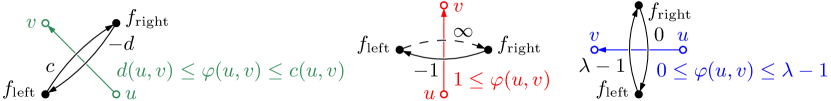
Figure 3: Definition of the dual edges for a flow network arc $a=(u,v)$ with demand $d(a)$ and capacity $c(a)$. Let $f_{\operatorname{left}}$ and $f_{\operatorname{right}}$ denote the vertices corresponding to the faces to the left and right of $a$ in $F_{\mathcal{G}}^{\lambda}$. Then add the edge $(f_{\operatorname{left}},f_{\operatorname{right}})$ with length $c(a)$ and the reverse edge $(f_{\operatorname{right}},f_{\operatorname{left}})$ with length $-d(a)$. Edges with infinite length are not created because they do not add constraints.

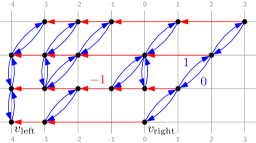
Figure 4: The distance network $D_{\mathcal{G}}^{2}$ obtained from the flow network $F_{\mathcal{G}}^{2}$ shown in Fig. 2 (c). The $x$-coordinate of every vertex is its distance from $v_{\operatorname{right}}$ in $D_{\mathcal{G}}^{2}$. All red arcs have length $-1$, all blue arcs pointing up have length $1$ and all blue arcs pointing down have length $0$. For every red arc there exists an arc in the reverse direction with length $\infty$. We omit these arcs because they do not impose any constraints on the shortest distance labeling.

A distance labeling is a function $x:V\to\mathbb{Z}$ that for every edge $(u,v)$ of $D_{\mathcal{G}}^{\lambda}$ with length $l$ satisfies $x(v)\leq x(u)+l$. We also say that $(u,v)$ imposes the distance constraint $x(v)\leq x(u)+l$. A distance labeling for $D_{\mathcal{G}}^{\lambda}$ is the $x$-coordinate assignment for a $\lambda$-drawing: For an edge $(u,v)$ of $D_{\mathcal{G}}^{\lambda}$ where $u,v$ are consecutive vertices in $\mathcal{G}$, the distance labeling guarantees $x(v)\leq x(u)-1$, i.e., the consecutive vertices are in the correct order and do not overlap. If an edge $(u,v)$ between layers has length $\lambda-1$, then the distance labeling ensures $x(v)\leq x(u)+\lambda-1$, i.e., $(u,v)$ has a slope in $\{0,\dots,\lambda-1\}$. Computing the shortest distances from $v_{\operatorname{right}}$ in $D_{\mathcal{G}}^{\lambda}$ to every vertex (if they are well-defined) gives a distance labeling that we refer to as the shortest distance labeling. A distance labeling of $D_{\mathcal{G}}^{\lambda}$ does not necessarily exist. This is the case when $D_{\mathcal{G}}^{\lambda}$ contains a negative cycle, e.g., when the in- or out-degree of a vertex in $\mathcal{G}$ is strictly larger than $\lambda$. For a distance labeling $x$ of $D_{\mathcal{G}}^{\lambda}$ we define a dual circulation $x^{\star}$ by setting $x^{\star}(a):=x(f_{\operatorname{right}})-x(f_{\operatorname{left}})$ for each arc $a$ of $F_{\mathcal{G}}^{\lambda}$ with left and right incident faces $f_{\operatorname{left}}$ and $f_{\operatorname{right}}$.

Lemma 3

Let $\mathcal{G}$ be an embedded level-planar graph and $\Gamma$ be a $\lambda$-drawing of $\mathcal{G}$. The function $x$ that assigns to each vertex of $\mathcal{G}$ its $x$-coordinate in $\Gamma$ is a distance labeling of $D_{\mathcal{G}}^{\lambda}$ and its dual $x^{\star}$ is a circulation in $F_{\mathcal{G}}^{\lambda}$.

Proof

Since $\Gamma$ preserves the embedding of $\mathcal{G}$, for each consecutive vertices $v,~{}u$, with $v$ preceeding $u$ in  $\mathcal{G}$ it holds that $\Gamma(v)<\Gamma(u)$. Since $\Gamma$ is a grid drawing  $\Gamma(v)\leq\Gamma(u)-1$, which implies $x(v)\leq x(u)+\ell$, where $\ell=-1$ is the length of $(u,v)$. Since  $\Gamma$ is a $\lambda$-drawing, i.e. every edge $(u,v)$ between the two levels has a slope in $\{0,\dots\lambda-1\}$, it holds that $\Gamma(u)\leq\Gamma(v)\leq\Gamma(u)+\lambda-1$, which implies $x(u)\leq x(v)+0$, for the edge $(v,u)$ of $D_{\mathcal{G}}^{\lambda}$ with length zero and $x(v)<x(u)+\lambda-1$ for the edge $(u,v)$ of $D_{\mathcal{G}}^{\lambda}$ with length $\lambda-1$. Hence, $x$ is a distance labeling of $D_{\mathcal{G}}^{\lambda}$.

We now show that $x^{\star}$ is a circulation in $F_{\mathcal{G}}^{\lambda}$. Let $f_{1},f_{2},\dots,f_{t},f_{t+1}=f_{1}$ be the faces incident to some node $v$ of $F_{\mathcal{G}}^{\lambda}$ in counter-clockwise order. Let $a$ be the arc incident to $v$ and dual to the edge between $f_{i}$ and $f_{i+1}$ with $1\leq i\leq t$. If $a$ is an incoming arc, it adds a flow of $x(f_{i+1})-x(f_{i})$ to $v$. If $a$ is an outgoing arc, it removes a flow of $x(f_{i})-x(f_{i+1})$ from $v$, or, equivalently, it adds a flow of $x(f_{i+1})-x(f_{i})$ to $v$. Therefore, the flow through $v$ is $\sum_{i}\left(x(f_{i+1})-x(f_{i})\right)$. This sum cancels to zero, i.e., the flow is preserved at $v$. Recall that the edge $(f_{\operatorname{left}},f_{\operatorname{right}})$ with length $c(a)$ in $D_{\mathcal{G}}^{\lambda}$ ensures $x(f_{\operatorname{right}})\leq x(f_{\operatorname{left}})+c(a)$, which gives $x^{\star}(a)\leq c(a)$. So, no capacities are exceeded. Analogously, the edge $(f_{\operatorname{right}},f_{\operatorname{left}})$ with length $-d(a)$ in $D_{\mathcal{G}}^{\lambda}$ ensures $x(f_{\operatorname{left}})\leq x(f_{\operatorname{right}})-d(a)$, which gives $x^{\star}(a)\geq d(a)$. Hence, all demands are fulfilled and $x^{\star}$ is indeed a circulation in $F_{\mathcal{G}}^{\lambda}$. ∎

Recall from Section 3 that for a circulation $\varphi$ in $F_{\mathcal{G}}^{\lambda}$ we define a dual drawing $\varphi^{\star}$ by setting the $x$-coordinates of the vertices of $\mathcal{G}$ as follows. For the lowest vertex of the right boundary set $\varphi^{\star}(v_{\operatorname{right}})=0$. Process the remaining vertices of the right boundary in ascending order with respect to their levels. Let $(u,v)$ be an edge of the right boundary so that $u$ has already been processed and $v$ has not been processed yet. Then set $\varphi^{\star}(v)=\varphi^{\star}(u)+\varphi((u,v)^{\star})$, where $(u,v)^{\star}$ is the slope arc dual to $(u,v)$. Let $w,x$ be a pair of consecutive vertices so that $x$ has already been processed and $w$ has not yet been processed yet. Then set $\varphi^{\star}(w)=\varphi^{\star}(x)+\varphi([w,x]^{\star})$, where $[w,x]^{\star}$ is a space arc. It turns out that $\varphi^{\star}$ is a distance labeling of $D_{\mathcal{G}}^{\lambda}$ and a $\lambda$-drawing of $\mathcal{G}$.

Lemma 4

Let $\mathcal{G}$ be an embedded level-planar graph, let $\lambda\in\mathbb{N}$, and let $\varphi$ be a circulation in $F_{\mathcal{G}}^{\lambda}$. The dual $\varphi^{\star}$ is a distance labeling of $D_{\mathcal{G}}^{\lambda}$ and the drawing induced by interpreting the distance label of a vertex as its $x$-coordinate is a $\lambda$-drawing of $\mathcal{G}$.

Proof

We show that $\varphi^{\star}$ is a distance labeling in $D_{\mathcal{G}}^{\lambda}$. The algorithm described above assings a value to every vertex of $D_{\mathcal{G}}^{\lambda}$. We now show that $\varphi^{\star}$ is indeed a distance labeling by showing that every edge satisfies a distance constraint.

Observe that the distance constraints imposed by edges dual to the space arcs are satisfied by construction. To show that the distance constraints imposed by edges dual to the slope arcs are also satisfied, we prove that for every edge $(u,v)$, it holds that $\varphi^{\star}(v)=\varphi^{\star}(u)+\varphi((u,v)^{\star})$. We refer to this as condition $\mathcal{C}$ for short. Since $\varphi((u,v)^{\star})\leq\lambda-1$ and the length $\ell$ of $(u,v)$ is $\lambda-1$ we obtain $\varphi^{\star}(v)=\varphi^{\star}(u)+\ell$, which implied that $\phi^{\star}$ is a distance labeling of $D_{\mathcal{G}}^{\lambda}$.

The proof is by induction based on the bottom to top and right to left order among the edges of $D_{\mathcal{G}}^{\lambda}$. We say that $(a,b)$ precedes $(c,d)$ if either $\ell(a)<\ell(c)$, or $\ell(a)=\ell(c)$ and $a$ is to the right of $c$, or $\ell(a)=\ell(c)$ and $b$ is to the right of $d$ (in case $a=c$). For the base case observe that the edges with both end-vertices on the first level and the edges of $p_{\operatorname{right}}$ satisfy condition $\mathcal{C}$ by the definition of $\varphi^{\star}$. Now let $(u,v)$ be an edge not addressed in the base case and assume that for every edge $(u^{\prime},v^{\prime})$ preceding edge $(u,v)$ condition $\mathcal{C}$ holds. For the inductive step we show that condition $\mathcal{C}$ also holds for $(u,v)$. Let $(u^{\prime},v^{\prime})$ denote the edge to the right of $(u,v)$ so that $(u,v)$ and $(u^{\prime},v^{\prime})$ are consecutive; see Fig. 5.

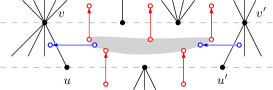
Figure 5: Proof of Lemma 4. Sets $A$ and $B$ contain the outgoing and incoming red flow network arcs incident to the gray oval, respectively.

Because $v$ is not the rightmost vertex on its level this edge exists. Let $A$ denote the set of space arcs $v_{1}v_{2}^{\star}$ in $F_{\mathcal{G}}^{\lambda}$ with $v_{1},v_{2}\in[v^{\prime},v]$. Analogously, let $B$ denote the set of space arcs $u_{1}u_{2}^{\star}$ in $F_{\mathcal{G}}^{\lambda}$ with $u_{1},u_{2}\in[u^{\prime},u]$. It is $\varphi^{\star}(v)=\varphi^{\star}(v^{\prime})+\sum_{a\in A}\varphi(a)$ by definition of $\varphi^{\star}$. Further, by induction hypothesis and since $(u^{\prime},v^{\prime})$ precedes $(u,v)$ it holds that $\varphi^{\star}(v^{\prime})=\varphi^{\star}(u^{\prime})+\varphi((u^{\prime},v^{\prime})^{\star})$. Inserting the latter into the former equation, we obtain $\varphi^{\star}(v)=\varphi^{\star}(u^{\prime})+\varphi((u^{\prime},v^{\prime})^{\star})+\sum_{a\in A}\varphi(a)$. Again, by definition of $\varphi^{\star}$, it is $\varphi^{\star}(u)=\varphi^{\star}(u^{\prime})+\sum_{b\in B}\varphi(b)$. By subtracting $\varphi^{\star}(u)$ from $\varphi^{\star}(v)$ we obtain

$$\varphi^{\star}(v)=\varphi^{\star}(u)-\sum_{b\in B}\varphi(b)+\varphi((u^{\prime},v^{\prime})^{\star})+\sum_{a\in A}\varphi(a)$$ (1)

Flow conservation on the vertex of $F_{\mathcal{G}}^{\lambda}$ to which edges of $A$ and $B$ are incident gives  $\varphi((u,v)^{\star})-\sum_{a\in A}\varphi(a)-\varphi((u^{\prime},v^{\prime})^{\star})+\sum_{b\in B}\varphi(b)=0$. Solving this equation for $\varphi(u,v)$ and inserting it into (1) yields $\varphi^{\star}(v)=\varphi^{\star}(u)+\varphi((u,v)^{\star})$, i.e. the condition $\mathcal{C}$ holds for $(u,v)$. Therefore $\varphi^{\star}$ is a distance labeling, which we have shown to define a $\lambda$-drawing of $\mathcal{G}$. ∎

Because $D_{\mathcal{G}}^{\lambda}$ is planar we can use the $O(n\log^{2}n/\log\log n)$-time shortest path algorithm due to Mozes and Wulff-Nilsen [28] to compute the shortest distance labeling. This improves our $O(n\log^{3}n)$-time algorithm from Section 3.

Theorem 4.1

Let $\mathcal{G}$ be an embedded proper level-planar graph. The distance labelings of $D_{\mathcal{G}}^{k}$ correspond bijectively to the $\lambda$-drawings of $\mathcal{G}$. If such a drawing exists, it can be found in $O(n\log^{2}n/\log\log n)$ time.

5 Partial and Simultaneous Drawings

In this section we use the distance model from Section 4 to construct partial and simultaneous  $\lambda$-drawings. We start with introducing a useful kind of drawing. Let $\Gamma$ be a $\lambda$-drawing of $\mathcal{G}$. We call $\Gamma$ a $\lambda$-rightmost drawing when there exists no $\lambda$-drawing $\Gamma^{\prime}$ with $\Gamma(v)<\Gamma^{\prime}(v)$ for some $v\in V$. In this definition, we assume $x(\Gamma(v_{\operatorname{right}}))=x(\Gamma^{\prime}(v_{\operatorname{right}}))=0$ to exclude trivial horizontal translations. Hence, a drawing is rightmost when every vertex is at its rightmost position across all level-planar $\lambda$-slope grid drawings of $\mathcal{G}$. It is not trivial that a $\lambda$-rightmost drawing exists, but it follows directly from the definition that if such a drawing exists, it is unique. The following lemma establishes the relationship between $\lambda$-rightmost drawings and shortest distance labelings of $D_{\mathcal{G}}^{\lambda}$.

Lemma 5

Let $\mathcal{G}$ be an embedded proper level-planar graph. If $D_{\mathcal{G}}^{\lambda}$ has a shortest distance labeling it describes the $\lambda$-rightmost drawing of $\mathcal{G}$.

Proof

The shortest distance labeling of $D_{\mathcal{G}}^{\lambda}$ is maximal in the sense that for any vertex $v$ there exists a vertex $u$ and an edge $(u,v)$ with length $l$ so that it is $x(v)=x(u)+l$. Recall that the definition of distance labelings only requires $x(v)\leq x(u)+l$. The claim then follows by induction over $V$ in ascending order with respect to the shortest distance labeling. ∎

5.1 Partial Drawings

Let $(\mathcal{G},\mathcal{H},\Pi)$ be a partial $\lambda$-drawing. In Section 3.1 we have shown that the flow model can be adapted to check whether $(\mathcal{G},\mathcal{H},\Pi)$ has a $\lambda$-extension, in case $\mathcal{H}$ is connected. In this section, we show how to adapt the distance model to extend partial $\lambda$-drawings, including the case $\mathcal{H}$ is disconnected. Recall that the distance label of a vertex $v$ is its $x$-coordinate. A partial $\lambda$-drawing fixes the $x$-coordinates of the vertices of $\mathcal{H}$. The idea is to express this with additional constraints in $D_{\mathcal{G}}^{\lambda}$. Let $v_{\operatorname{ref}}$ be a vertex of $\mathcal{H}$. In a $\lambda$-extension of $(\mathcal{G},\mathcal{H},\Pi)$, the relative distance along the $x$-axis between a vertex $v$ of $\mathcal{H}$ and vertex $v_{\operatorname{ref}}$ should be $d_{v}=\Pi(v_{\operatorname{ref}})-\Pi(v)$. This can be achieved by adding an edge $(v,v_{\operatorname{ref}})$ with length $d_{v}$ and an edge $(v_{\operatorname{ref}},v)$ with length $-d_{v}$. The first edge ensures that it is $x(v_{\operatorname{ref}})\leq x(v)+d_{v}$, i.e., $x(v)\geq x(v_{\operatorname{ref}})-d_{v}$ and the second edge ensures $x(v)\leq x(v_{\operatorname{ref}})-d$. Together, this gives $x(v)=x(v_{\operatorname{ref}})-d_{v}$. Let $D_{{\mathcal{G}},\Pi}^{\lambda}$ be $D_{\mathcal{G}}^{\lambda}$ augmented by the edges $\{(v,v_{\operatorname{ref}}),(v_{\operatorname{ref},v}):\forall v\in{\mathcal{H}}\}$ with lengths as described above.

To decide existence of $\lambda$-extension and in affirmative construct the corresponding drawing we compute the shortest distance labeling in $D_{{\mathcal{G}},\Pi}^{\lambda}$. Observe that this network can contain negative cycles and therefore no shortest distance labeling. Unfortunately, $D_{{\mathcal{G}},\Pi}^{\lambda}$ is not planar, and thus we cannot use the embedding-based algorithm of Mozes and Wulff-Nilsen. However, since all newly introduced edges have $v_{\operatorname{ref}}$ as one endpoint, $v_{\operatorname{ref}}$ is an apex of $D_{\mathcal{G}}^{\lambda}$, i.e., removing $v_{\operatorname{ref}}$ from $D_{{\mathcal{G}},\Pi}^{\lambda}$ makes it planar. Therefore $D_{{\mathcal{G}},\Pi}^{\lambda}$ can be recursively separated by separators of size $O(\sqrt{n})$. We can therefore use the shortest-path algorithm due to Henzinger et al. to compute the shortest distance labeling of $D_{{\mathcal{G}},\Pi}^{\lambda}$ in $O(n^{4/3}\log n)$ time [16].

Theorem 5.1

Let $(\mathcal{G},\mathcal{H},\Pi)$ be a partial $\lambda$-drawing. In $O(n^{4/3}\log n)$ time it can be determined whether $(\mathcal{G},\mathcal{H},\Pi)$ has a $\lambda$-extension and in the affirmative the corresponding drawing can be computed within the same running time.

5.2 Simultaneous Drawings

In the simultaneous $\lambda$-drawing problem, we are given a tuple $(\mathcal{G}_{1},\mathcal{G}_{2})$ of two embedded level-planar graphs that share a common subgraph $\mathcal{G}_{1\cap 2}=\mathcal{G}_{1}\cap\mathcal{G}_{2}$. We assume w.l.o.g. that $G_{1}$ and $G_{2}$ share the same right boundary and that the embeddings of $\mathcal{G}_{1}$ and $\mathcal{G}_{2}$ coincide on $\mathcal{G}_{1\cap 2}$. The task is to determine whether there exist $\lambda$-drawings $\Gamma_{1},\Gamma_{2}$ of $\mathcal{G}_{1},\mathcal{G}_{2}$, respectively, so that $\Gamma_{1}$ and $\Gamma_{2}$ coincide on the shared graph $\mathcal{G}_{1\cap 2}$. The approach is the following. Start by computing the rightmost drawings of $\mathcal{G}_{1}$ and $\mathcal{G}_{2}$. Then, as long as these drawings do not coincide on $\mathcal{G}_{1\cap 2}$ add necessary constraints to $D_{\mathcal{G}_{1}}^{\lambda}$ and $D_{\mathcal{G}_{2}}^{\lambda}$. This process terminates after a polynomial number of iterations, either by finding a simultaneous $\lambda$-drawing, or by determining that no such drawing exist.

Finding the necessary constraints works as follows. Suppose that $\Gamma_{1},\Gamma_{2}$ are the rightmost drawings of $\mathcal{G}_{1},\mathcal{G}_{2}$, respectively. Because both $\mathcal{G}_{1}$ and $\mathcal{G}_{2}$ have the same right boundary they both contain vertex $v_{\operatorname{right}}$. We define the coordinates in the distance labelings of $D_{\mathcal{G}_{1}}^{\lambda}$ and $D_{\mathcal{G}_{2}}^{\lambda}$ in terms of this reference vertex.

Now suppose that for some vertex $v$ of $\mathcal{G}_{1\cap 2}$ the $x$-coordinates in $\Gamma_{1}$ and $\Gamma_{2}$ differ, i.e., it is $\Gamma_{1}(v)\neq\Gamma_{2}(v)$. Assume $\Gamma_{1}(v)<\Gamma_{2}(v)$ without loss of generality. Because $\Gamma_{1}$ is a rightmost drawing, there exists no drawing of $\mathcal{G}_{1}$ where $v$ has an $x$-coordinate greater than $\Gamma_{1}(v)$. In particular, there exist no simultaneous drawings where $v$ has an $x$-coordinate greater than $\Gamma_{1}(v)$. Therefore, we must search for a simultaneous drawing where $\Gamma_{2}(v)\leq\Gamma_{1}(v)$. We can enforce this constraint by adding an edge $(v_{\operatorname{right}},v)$ with length $\Gamma_{1}(v)$ into $D_{\mathcal{G}_{2}}^{\lambda}$. We then attempt to compute the drawing $\Gamma_{2}$ of $\mathcal{G}_{2}$ defined by the shortest distance labeling in $D_{\mathcal{G}_{2}}^{\lambda}$. This attempt produces one of two possible outcomes. The first possibility is that there now exists a negative cycle in $D_{\mathcal{G}_{2}}^{\lambda}$. This means that there exists no drawing $\Gamma_{2}$ of $G_{2}$ with $\Gamma_{2}(v)\leq\Gamma(v)$. Because $\Gamma_{1}$ is a rightmost drawing, this means that no simultaneous drawings of $\mathcal{G}_{1}$ and $\mathcal{G}_{2}$ exist. The algorithm then terminates and rejects this instance. The second possiblity is that we obtain a new drawing $\Gamma_{2}$. This drawing is rightmost among all drawings that satisfy the added constraint $\Gamma_{2}(v)\leq\Gamma_{1}(v)$. In this case there are again two possibilities. Either we have $\Gamma_{1}(v)=\Gamma_{2}(v)$ for each vertex $v$ in $\mathcal{G}_{1\cap 2}$. In this case $\Gamma_{1}$ and $\Gamma_{2}$ are simultaneous drawings and the algorithm terminates. Otherwise there exists at least one vertex $w$ in $\mathcal{G}_{1\cap 2}$ with $\Gamma_{1}(w)\neq\Gamma_{2}(w)$. We then repeat the procedure just described for adding a new constraint.

We repeat this procedure of adding other constraints. To bound the number of iterations, recall that we only consider compact drawings, i.e., drawings whose width is at most $(\lambda-1)(n-1)$. In each iteration the $x$-coordinate of at least one vertex is decreased by at least one. Therefore, each vertex is responsible for at most $(\lambda-1)(n-1)$ iterations. The total number of iterations is therefore bounded by $n(\lambda-1)(n-1)\in O(\lambda n^{2})$.

Note that due to the added constraints $D_{\mathcal{G}_{1}}^{\lambda}$ and $D_{\mathcal{G}_{2}}^{\lambda}$ are generally not planar. We therefore apply the $O(n^{4/3}\log n)$-time shortest-path algorithm due to Henzinger et al. that relies not on planarity but on $O(\sqrt{n})$-sized separators to compute the shortest distance labellings. This gives the following.

Theorem 5.2

Let $\mathcal{G}_{1},\mathcal{G}_{2}$ be embedded level-planar graphs that share a common subgraph $\mathcal{G}_{1\cap 2}$. In $O(\lambda n^{10/3}\log n)$ time it can be determined whether $\mathcal{G}_{1},\mathcal{G}_{2}$ admit simultaneous $\lambda$-drawings and if so, such drawings can be computed within the same running time.

6 Conclusion

In this paper we studied $\lambda$-drawings, i.e., level-planar drawings with $\lambda$ slopes. We model $\lambda$-drawings of proper level-planar graphs as integer flow networks. This lets us find $\lambda$-drawings and extend connected partial  $\lambda$-drawings in $O(n\log^{3}n)$ time. We extend the duality between integer flows in a primal graph and shortest distances in its dual to obtain a more powerful distance model. This distance model allows us to find $\lambda$-drawings in $O(n\log^{2}n/\log\log n)$ time, extend not-necessarily-connected partial  $\lambda$-drawings in $O(n^{4/3}\log n)$ time and find simultaneous  $\lambda$-drawings in $O(\lambda n^{10/3}\log n)$ time.

In the non proper case, testing the existence of a $2$-drawing becomes NP-hard, even for biconnected graphs with maximum edge length two; see Appendix 0.A.

Appendix 0.A Complexity of the General Case

So far, we have considered proper level graphs, i.e., level graphs where all edges have length one. In this section, we consider the general case, where edges may have arbitrary lengths. We say that an edge with length two or more is long. One approach would be to try to adapt the flow model from Section 3 to this more general case. By subdividing long edges, any level graph $G$ can be transformed into a proper level graph $G^{\prime}$. Observe that two edges in $G^{\prime}$ created by subdividing the same long edge must have the same slope in order to yield a fixed-slope drawing of $G$. In the context of our flow model, this means that the amount of flow across the corresponding slope arcs must be the same. Our problem then becomes an instance of the integer equal flow problem. In this problem, we are given a flow network along with disjoint sets $R_{1},R_{2},\dots,R_{t}$ of arcs. The task is to find the maximum flow from $s$ to $t$ such that the amount of flow across arcs in the same set $R_{i}$ is the same. This problem was introduced and shown to be NP-hard by Sahni [34]. The problem remains NP-hard in special cases [12, 35] and the integrality gap of the fractional LP can be arbitrarily large [27].

In this section we show that the level-planar grid drawing problem is NP-complete even for two slopes and biconnected graphs where all edges have length one or two. To this end, we present a reduction from rectilinear planar monotone 3-Sat [8]. An instance of this problem consists of a set of variables $X$ and a set of clauses $C$. A clause is positive (negative) when it consists of only positive (negative) literals. We say that the instance is monotone when each clause is either positive or negative. Further, the instance can be planarly drawn as a graph with vertices $X\cup C$; see Fig. 6.

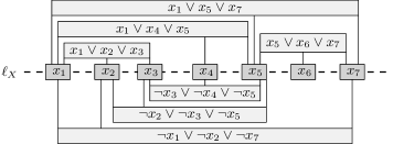
Figure 6: An instance of planar monotone 3-Sat.

In this drawing, the variables are aligned along a virtual horizontal line $\ell_{X}$. Positive clauses are drawn as vertices above $\ell_{X}$ and connected by an edge to a variable if the clause contains the corresponding postive literal. Symmetrically, negative clauses are drawn as vertices below $\ell_{X}$ and connected by an edge to a variable if the clause contains the corresponding negative literal.

Our reduction works by first replacing every vertex that corresponds to a variable by a variable gadget and every vertex that corresponds to a positive (negative) clause by a positive (negative) clause gadget. All three gadgets consist of fixed and movable parts. The fixed parts only admit one level-planar two-slope grid drawing, whereas the movable parts admit two or more drawings depending on the choice of slope for some edges. Second, the gadgets are connected by a common fixed frame. All fixed parts of the gadgets are connected to the common frame in order to provide a common point of reference. The movable parts of the gadgets then interact in such a way that any level-planar two-slope grid drawing induces a solution to the underlying planar monotone 3-Sat instance.

The variable gadget consists of a number of connectors arranged around a fixed horizontal line that connects all variable gadgets along the virtual line of variables $\ell_{X}$. See Fig. 7, where the fixed structure is shaded in gray.

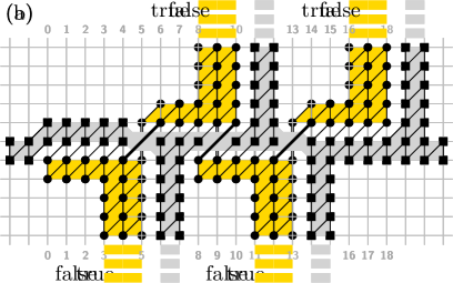
Figure 7: The variable gadget drawn in the “true” configuration (a) and the “false” configuration (b).

Vertices drawn as squares are fixed, i.e., they cannot change their position relative to other vertices drawn as squares. Vertices drawn as circles are movable, i.e., they can change their position relative to vertices drawn as squares. The line of variables $\ell_{X}$ extends from the the square vertices on the left and right boundaries of the drawing. Every connector consists of two pins: the movable assignment pin and the fixed reference pin. The variable gadget in Fig. 7 features four connectors: two above the horizontal line and two below the horizontal line. Assignment pins are shaded in yellow and reference pins are shaded in gray. The relative position of the assignment pin and the reference pin of one connector encodes the truth assignment of the underlying variable. Moreover, the reference pin allows the fixed parts of the clause gadgets to be connected to the variable gadgets and thereby to the common frame. Comparing Fig. 7 (a) and (b), observe how the relative position of the two pins of each connector changes depending on the truth assignment of the underlying variable. The key structure of the variable gadget is that the position of the assignment pins of one variable gadget are coordinated by long edges. In Fig. 7, long edges are drawn as thick lines. Changing the slope of these long edges moves all assignment pins above the horizontal line in one direction and all assignment pins below the horizontal line in the reverse direction. In this way, all connectors encode the same truth assignment of the underlying variable. Note that we can introduce as many connectors as needed for any one variable.

The positive clause gadget consists of a fixed boundary, a movable wiggle and three assignment pin endings. See Fig. 8, where the fixed boundary is shaded in gray, the wiggle is highlighted in blue and the assignment pin endings are highlighted in yellow.

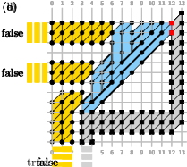
Figure 8: The positive clause gadget. Subfigures (a)–(c) show the drawing when at least one variable is assigned to true. Subfigure (d) shows that no drawing exists when all variables are assigned to false, because this leads to intersections, e.g., at the vertices marked in red.

The fixed boundary is connected to the reference pin of the variable gadget that is rightmost amongst the connected variable gadgets. Because the variable gadgets are fixed to the common frame, the boundary of the positive clause gadget is also connected to the common frame. The assignment pin endings are connected to assigment pins of connectors of the corresponding variable gadgets. The idea of the positive clause gadget is that the wiggle has to wiggle through the space bounded by the assignment pin endings on the left and the fixed boundary on the right. Recall that the assignment pins change their horizontal position depending on the truth assignment of their underlying variables. The positive clause gadget is designed so that the wiggle can always be drawn, except for the case when all variables are assigned to false. See Fig. 8 (a)–(c), which shows the three possible situations when exactly one variable is assigned to true. In any case where at least one variable is assigned to true the wiggle can be drawn in one of the three ways shown. However, as shown in Fig. 8 (d), the wiggle cannot be drawn in the case where all variables are assigned to false. The reason for this is that the the assignment pin endings get so close to the fixed boundary that they leave too little space for the wiggle to be drawn. This means that some vertices must intersect, for example those shown in red in Fig. 8 (d).

The negative clause gadgets works very similarly. It is drawn below the horizontal line of variables and it forces at least one of the incident variable gadgets to be configured as false. See Fig. 9, where subfigures (a)–(c) show the admissible drawings and subfigure (d) shows that the case when all incident variables are configured as true cannot occur.

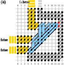
Figure 9: The negative clause gadget. Subfigures (a)–(c) show the drawing when at least one variable is assigned to false. Subfigure (d) shows that no drawing exists when all variables are assigned to true, because this leads to intersections, e.g., at the vertices marked in red. Note the symmetry to the positive clause gadget in Fig. 8.

Note that this uses the design of the variable gadget that the assignment and reference pins below the horizontal line are closer when the variable is assigned to true (i.e., the inverse situtation compared to the situation above the horizontal line).

It is evident that any level-planar two-slope grid drawing of the resulting graph induces a solution of the underlying planar monotone 3-Sat problem and vice versa. Note that the variable gadgets become biconnected when embedded into the common frame and that the clause gadgets are biconnected by design. Furthermore, all long edges have length two. We therefore conclude the following.

Theorem 0.A.1

The level-planar grid drawing problem is NP-complete even for two slopes and biconnected graphs where all edges have length one or two.

References

- [1] FAUSTEDITION. http://www.faustedition.net/macrogenesis/dag.
- [2] Patrizio Angelini, Steven Chaplick, Sabine Cornelsen, Giordano Da Lozzo, Giuseppe Di Battista, Peter Eades, Philipp Kindermann, Jan Kratochvíl, Fabian Lipp, and Ignaz Rutter. Simultaneous orthogonal planarity. In Yifan Hu and Martin Nöllenburg, editors, Proceedings of the 24th International Symposium on Graph Drawing and Network Visualization, pages 532–545. Springer, Cham, 2016.
- [3] Patrizio Angelini, Giordano Da Lozzo, Giuseppe Di Battista, Fabrizio Frati, Maurizio Patrignani, and Ignaz Rutter. Beyond level planarity. In Yifan Hu and Martin Nöllenburg, editors, Proceedings of the 24th International Symposium on Graph Drawing and Network Visualization, pages 482–495. Springer, Cham, 2016.
- [4] János Barát, Jivr’i Matouvsek, and David R. Wood. Bounded-degree graphs have arbitrarily large geometric thickness. Electr. J. Comb., 13(1), 2006.
- [5] Thomas Bläsius, Stephen G. Kobourov, and Ignaz Rutter. Simultaneous embedding of planar graphs. In Tamassia [36], pages 349–381.
- [6] Glencora Borradaile, Philip N. Klein, Shay Mozes, Yahav Nussbaum, and Christian Wulff-Nilsen. Multiple-source multiple-sink maximum flow in directed planar graphs in near-linear time. In Proceedings of the 52nd Annual IEEE Symposium on Foundations of Computer Science, pages 170–179. IEEE Press, New York, 2011.
- [7] Guido Brückner and Ignaz Rutter. Partial and constrained level planarity. In Philip N. Klein, editor, Proceedings of the 28th Annual ACM-SIAM Symposium on Discrete Algorithms, pages 2000–2011. SIAM, 2017.
- [8] Mark de Berg and Amirali Khosravi. Optimal binary space partitions in the plane. In My T. Thai and Sartaj Sahni, editors, Proceedings of the 16th International Computing and Combinatorics Conference, pages 216–225. Springer, Berlin, Heidelberg, 2010.
- [9] Emilio Di Giacomo, Giuseppe Liotta, and Fabrizio Montecchiani. Drawing outer 1-planar graphs with few slopes. Journal of Graph Algorithms and Applications, 19(2):707–741, 2015.
- [10] Vida Dujmović, David Eppstein, Matthew Suderman, and David R. Wood. Drawings of planar graphs with few slopes and segments. Computational Geometry, 38(3):194–212, October 2007.
- [11] Vida Dujmović, Matthew Suderman, and David R. Wood. Graph drawings with few slopes. Computational Geometry, 38(3):181–193, October 2007.
- [12] Shimon Even, Alon Itai, and Adi Shamir. On the complexity of timetable and multicommodity flow problems. SIAM Journal on Computing, 5(4):691–703, December 1976.
- [13] Emilio Di Giacomo, Giuseppe Liotta, and Fabrizio Montecchiani. Drawing subcubic planar graphs with four slopes and optimal angular resolution. Theor. Comput. Sci., 714:51–73, 2018.
- [14] Refael Hassin. Maximum flow in planar networks. Information Processing Letters, 13(3):107, December 1981.
- [15] Patrick Healy and Nikola S. Nikolov. Hierarchical drawing algorithms. In Tamassia [36], pages 409–453.
- [16] Monika R. Henzinger, Philip N. Klein, Satish Rao, and Sairam Subramanian. Faster shortest-path algorithms for planar graphs. Journal of Computer and System Sciences, 55(1):3–23, August 1997.
- [17] Udo Hoffmann. On the complexity of the planar slope number problem. J. Graph Algorithms Appl., 21(2):183–193, 2017.
- [18] Te Chiang Hu. Integer Programming and Network Flows. Addison-Wesley, Reading, MA, 1969.
- [19] Alon Itai and Yossi Shiloach. Maximum flow in planar networks. SIAM Journal on Computing, 8(2):135–150, May 1979.
- [20] Stefan Jänicke, Annette Geßner, Greta Franzini, Melissa Terras, Simon Mahony, and Gerik Scheuermann. Traviz: A visualization for variant graphs. DSH, 30(Suppl-1):i83–i99, 2015.
- [21] Balázs Keszegh, János Pach, and Dömötör Pálvölgyi. Drawing planar graphs of bounded degree with few slopes. SIAM Journal on Discrete Mathematics, 27(2):1171–1183, June 2013.
- [22] Balázs Keszegh, János Pach, Dömötör Pálvölgyi, and Géza Tóth. Drawing cubic graphs with at most five slopes. Computational Geometry, 40(2):138–147, July 2008.
- [23] Philipp Kindermann, Wouter Meulemans, and André Schulz. Experimental analysis of the accessibility of drawings with few segments. Journal of Graph Algorithms and Applications, 22(3):501–518, 2018.
- [24] Kolja B. Knauer, Piotr Micek, and Bartosz Walczak. Outerplanar graph drawings with few slopes. Comput. Geom., 47(5):614–624, 2014.
- [25] William Lenhart, Giuseppe Liotta, Debajyoti Mondal, and Rahnuma Islam Nishat. Planar and plane slope number of partial 2-trees. In Stephen K. Wismath and Alexander Wolff, editors, Graph Drawing - 21st International Symposium, GD 2013, Bordeaux, France, September 23-25, 2013, Revised Selected Papers, volume 8242 of Lecture Notes in Computer Science, pages 412–423. Springer, 2013.
- [26] Tamara Mchedlidze, Martin Nöllenburg, and Ignaz Rutter. Extending convex partial drawings of graphs. Algorithmica, 76(1):47–67, September 2016.
- [27] Carol Meyers and Andreas Schulz. Integer equal flows. Operations Research Letters, 37(4):245–249, July 2009.
- [28] Shay Mozes and Christian Wulff-Nilsen. Shortest paths in planar graphs with real lengths in time. In Mark de Berg and Ulrich Meyer, editors, Proceedings of the 18th Annual European Conference on Algorithms, pages 206–217. Springer, Berlin, Heidelberg, 2010.
- [29] Soeren Nickel and Martin Nöllenburg. Drawing -linear Metro Maps. CoRR, abs/1904.03039, 2019.
- [30] Martin Nöllenburg. A survey on automated metro map layout methods. In Schematic Mapping Workshop. Essex, UK, April 2014.
- [31] János Pach and Dömötör Pálvölgyi. Bounded-degree graphs can have arbitrarily large slope numbers. Electr. J. Comb., 13(1), 2006.
- [32] Maurizio Patrignani. On extending a partial straight-line drawing. Int. J. Found. Comput. Sci., 17(5):1061–1070, 2006.
- [33] Helen C. Purchase. Metrics for graph drawing aesthetics. J. Vis. Lang. Comput., 13(5):501–516, 2002.
- [34] Sartaj Sahni. Computationally related problems. SIAM Journal on Computing, 3(4):262–279, December 1974.
- [35] K. Srinathan, Pranava R. Goundan, M. V. N. Ashwin Kumar, R. Nandakumar, and C. Pandu Rangan. Theory of equal-flows in networks. In Oscar H. Ibarra and Louxin Zhang, editors, Proceedings of the 8th International Computing and Combinatorics Conference, pages 514–524. Springer, Berlin, Heidelberg, 2002.
- [36] Roberto Tamassia, editor. Handbook on Graph Drawing and Visualization. Chapman and Hall/CRC, 2013.