Evolutionary Dataset Optimisation: learning algorithm quality through evolution

Abstract

In this paper we propose a novel method for learning how algorithms perform. Classically, algorithms are compared on a finite number of existing (or newly simulated) benchmark datasets based on some fixed metrics. The algorithm(s) with the smallest value of this metric are chosen to be the ‘best performing’. We offer a new approach to flip this paradigm. We instead aim to gain a richer picture of the performance of an algorithm by generating artificial data through genetic evolution, the purpose of which is to create populations of datasets for which a particular algorithm performs well on a given metric. These datasets can be studied so as to learn what attributes lead to a particular progression of a given algorithm. Following a detailed description of the algorithm as well as a brief description of an open source implementation, a case study in clustering is presented. This case study demonstrates the performance and nuances of the method which we call Evolutionary Dataset Optimisation. In this study, a number of known properties about preferable datasets for the clustering algorithms known as $k$-means and DBSCAN are realised in the generated datasets.

1 Introduction

This work presents a novel approach to learning the quality and performance of an algorithm through the use of evolution. When an algorithm is developed to solve a given problem, the designer is presented with questions about the performance of their proposed method and its relative performance against existing methods. This is an inherently difficult task. However, under the current paradigm, the standard response to this situation is to use a known fixed set of datasets - or simulate new datasets themselves - and a common metric amongst the proposed method and its competitors. The collated algorithms are then assessed based on this metric with often minimal consideration for the appropriateness or reliability of the datasets being used, and the robustness of the method(s) in question [1, 13, 19].

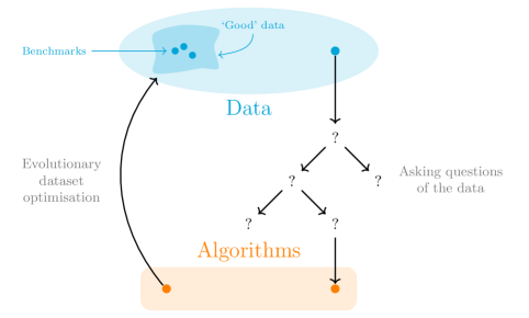
This process is not so readily observed when travelling in the opposite direction but methods to do so exist. Suppose that the object of interest was not an algorithm but rather a dataset. In this case, the objective is to determine a preferable algorithm to complete some task on the data. There exist a number of methods employed across disciplines to complete this task that take into account the characteristics of the data and the context of the research problem. These methods are often equivalent to asking questions of the data, and include the use of diagnostic tests. For instance, in the case of clustering, if the data displayed an indeterminate number of non-convex blobs, then one could recommend that an appropriate clustering algorithm would be DBSCAN [11]. Otherwise, for scalability, $k$-means may be chosen [37, 38].

The approach presented in this work aims to flip the paradigm described here by allowing the data itself to be unfixed. This fluidity in the data is achieved by generating data for which the algorithm performs well (or better than some other) through the use of an evolutionary algorithm. The purpose of doing so is not to simply create a bank of useful datasets but rather to allow for the subsequent studying of these datasets. In doing so, the attributes and characteristics which lead to the success (or failure) of the algorithm may be described, giving a broader understanding of the algorithm on the whole. Our framework is described in Figure 1.

Figure 1: On the right: the current path for selecting some algorithm(s) based on their validity and performance for a given dataset. On the left: the proposed flip to better understand the space in which ‘good’ datasets exist for an algorithm.

This proposed flip has a number of motivations, and below is a non-exhaustive list of some of the problems that are presented by the established evaluation paradigm:

1. How are these benchmark examples selected? There is no true measure of their reliability other than their frequent use. In some domains and disciplines there are well-established benchmarks so those found through literature may well be reliable, but in others less so [5, 8, 36].

2. Sometimes, when there is a lack of benchmark examples, a ‘new’ dataset is simulated to assess the algorithm [26]. This begs the question as to how and why that simulation is created. Not only this, but the origins of existing benchmarks is often a matter of convenience rather than their merit.

3. In disciplines where there are established benchmarks, there may still be underlying problems around the true performance of an algorithm:

   1. As an example, work by Torralba and Efros [34] showed that image classifiers trained and evaluated on a particular dataset, or datasets, did not perform reliably when evaluated using other benchmark datasets that were determined to be similar. Thus leading to a model which lacks robustness.

   2. The amount of learning one can gain as to the characteristics of data which lead to good (or bad) performance of an algorithm is constrained to the finite set of attributes present in the benchmark data chosen in the first place.

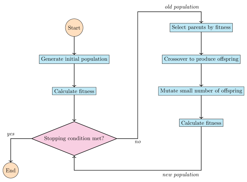
This work presents just one method from this new paradigm, and that method is built around the concept of evolution. Evolutionary algorithms (EAs) have been applied successfully to solve a wide array of problems - particularly where the complexity of the problem or its domain are significant. These methods are highly adaptive and their population-based construction (displayed in Figure 2) allows for the efficient solving of problems that are otherwise beyond the scope of traditional search and optimisation methods. EAs have been chosen here as they are simple in design yet their capabilities encompass the difficulties of the flipped paradigm set out above.

Figure 2: A general schematic for an evolutionary algorithm.

The use of EAs to generate artificial data is not a new concept, however. Its applications in data generation have included developing methods for the automated testing of software [16, 23, 29] and the synthesis of existing or confidential data [6]. Such methods also have a long history in the parameter optimisation of algorithms, and recently in the automated design of convolutional neural network (CNN) architecture [31, 32].

Other methods for the generation or synthesis of artificial data are numerous and range from simple concepts such as simulated annealing [21] to swarm-based learning techniques [2] or generative adversarial networks (GANs) [12]. The unconstrained learning style of methods such as CNNs and GANs aligns with that proposed in this work. By allowing the EA to explore and learn about the search space in an organic way, less-prejudiced insight can be established that is not necessarily reliant on any particular framework or agenda.

Note that the proposed methodology is not simply to use an EA to optimise an algorithm over a search space with fixed dimension or data type such as those set out in [6]. The shape of a dataset is considered a part of the sample space itself that can be traversed through the evolutionary algorithm.

The remainder of the paper is structured as follows:

• Section 2 describes the structure of the proposed method including its parameters and operators.

• Section 3 contains a case study where the success and failure of $k$-means clustering is examined using the proposed method. Included also is a comparison between $k$-means and another clustering algorithm DBSCAN.

• Section 4 concludes this paper.

2 The evolutionary algorithm

In this section, the details of an algorithm that generates data for which a given function, or (equivalently) algorithm, is well-suited is described. This algorithm is to be referred to as “Evolutionary Dataset Optimisation” (EDO).

The EDO method is built as an evolutionary algorithm which follows a traditional (generic) schema with some additional features that keep the objective of artificial data generation in mind. With that, there are a number of parameters that are passed to EDO; the typical parameters of an evolutionary algorithm are a fitness function, $f$, which maps from an individual to a real number, as well as a population size, $N$, a maximum number of iterations, $M$, a selection parameter, $b$, and a mutation probability, $p_{m}$. In addition to these, EDO takes the following parameters:

• A set of probability distribution families, $\mathcal{P}$. Each family in this set has some parameter limits which form a part of the overall search space. For instance, the family of normal distributions, denoted by $N(\mu,\sigma^{2})$, would have limits on values for the mean, $\mu$, and the standard deviation, $\sigma$.

• A maximum number of “subtypes” for each family in $\mathcal{P}$. A subtype is an independent copy of the family that progresses separate from the others. These are the actual distribution objects which are traversed in the optimisation.

• A probability vector to sample distributions from $\mathcal{P}$, $w=\left(w_{1},\ldots,w_{|\mathcal{P}|}\right)$.

• Limits on the number of rows an individual dataset can have,

  $$R\in\left\{(r_{\min},r_{\max})\in\mathbb{N}^{2}~{}|~{}r_{\min}\leq r_{\max}\right\}$$

• Limits on the number of columns a dataset can have,

  $$C:=\left(C_{1},\ldots,C_{|\mathcal{P}|}\right)\text{ where }C_{j}\in\left\{(c_{\min},c_{\max})\in{\left(\mathbb{N}\cup\{\infty\}\right)}^{2}~{}|~{}c_{\min}\leq c_{\max}\right\}$$

  for each $j=1,\ldots,|\mathcal{P}|$. That is, $C$ defines the minimum and maximum number of columns a dataset may have from each distribution in $\mathcal{P}$.

• A second selection parameter, $l\in[0,1]$, to allow for a small proportion of ‘lucky’ individuals to be carried forward.

• A shrink factor, $s\in[0,1]$, defining the relative size of a component of the search space to be retained after adjustment.

The concepts discussed in this section form the mechanisms of the evolutionary dataset optimisation algorithm. To use the algorithm practically, these components have been implemented in Python as a library built on the scientific Python stack [22, 25]. The library is fully tested and documented (at https://edo.readthedocs.io) and is freely available online under the MIT license [33]. The EDO implementation was developed to be consistent with the current best practices of open source software development [15].

Input: $f,N,R,C,\mathcal{P},w,M,b,l,p_{m},s$

Output: A full history of the populations and their fitnesses.

begin

      create initial population of individuals

       find fitness of each individual

       record population and its fitness

      

      while current iteration less than the maximum and stopping condition not met  do

            select parents based on fitness and selection proportions

             use parents to create new population through crossover and mutation

             find fitness of each individual

             update population and fitness histories

             if adjusting the mutation probability then

                  update mutation probability

             end if

            if using a shrink factor then

                  shrink the mutation space based on parents

             end if

            

       end while

      

end

Algorithm 1 The Evolutionary Dataset Optimisation algorithm

Input: parents, $N,R,C,\mathcal{P},w,p_{m}$

Output: A new population of size $N$

begin

      add parents to the new population

       while the size of the new population is less than $N$ do

            sample two parents at random

             create an offspring by crossing over the two parents

             mutate the offspring according to the mutation probability

             add the mutated offspring to the population

            

       end while

      

end

Algorithm 2 Creating a new population

The statement of the EDO algorithm is presented here to lay out its general structure from a high level perspective. Lower level discussion is provided below where additional algorithms for the individual creation, evolutionary operator and shrinkage processes are given along with diagrams (where appropriate). Note that there are no defined processes for how to stop the algorithm or adjust the mutation probability, $p_{m}$. This is down to their relevance to a particular use case. Some examples include:

• Regular decreasing in mutation probability across the available attributes [17].

• Stopping when no improvement in the best fitness is found within some $K$ consecutive iterations [18].

• Utilising global behaviours in fitness to indicate a stopping point [20].

2.1 Individuals

Evolutionary algorithms operate in an iterative process on populations of individuals that each represent a solution to the problem in question. In a genetic algorithm, an individual is a solution encoded as a bit string of, typically, fixed length and treated as a chromosome-like object to be manipulated. In EDO, as the objective is to generate datasets and explore the space in which datasets exist, there is no encoding. As such the distinction is made that EDO is an evolutionary algorithm.

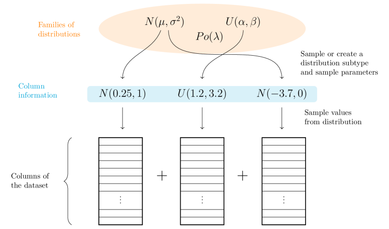
As is seen in Figure 3, an individual’s creation is defined by the generation of its columns. A set of instructions on how to sample new values (in mutation, for instance, Section 2.4) for that column are recorded in the form of a probability distribution. These distributions are sampled and created from the families passed in $\mathcal{P}$. In EDO, the produced datasets and their metadata are manipulated directly so that the biological operators can be designed and be interpreted in a more meaningful way as will be seen later in this section.

However, one should not assume that the columns are a reliable representative of the distribution associated with them, or vice versa. This is particularly true of ‘shorter’ datasets with a small number of rows, whereas confidence in the pair could be given more liberally for ‘longer’ datasets with a larger number of rows. In any case, appropriate methods for analysis should be employed before formal conclusions are made.

Figure 3: An example of how an individual is first created.

Input: $R,C,\mathcal{P},w$

Output: An individual defined by a dataset and some metadata

begin

      sample a number of rows and columns

       create an empty dataset

       for each column in the dataset do

            sample a distribution from $\mathcal{P}$

             create an instance of the distribution

             fill in the column by sampling from this instance

             record the instance in the metadata

       end for

      

end

Algorithm 3 Creating an individual

2.2 Selection

The selection operator describes the process by which individuals are chosen from the current population to generate the next. Almost always, the likelihood of an individual being selected is determined by their fitness. This is because the purpose of selection is to preserve favourable qualities and encourage some homogeneity within future generations [4].

Figure 4: The selection process with the inclusion of some lucky individuals.

Input: population, population fitness, $b$, $l$

Output: A set of parent individuals

begin

      calculate $n_{b}$ and $n_{l}$

       sort the population by the fitness of its individuals

       take the first $n_{b}$ individuals and make them parents

       if there are any individuals left then

            take the next $n_{l}$ individuals and make them parents

            

       end if

      

end

Algorithm 4 The selection process

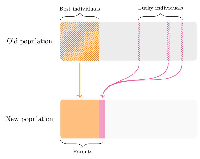
In EDO, a modified truncation selection method is used [14], as can be seen in Figure 4. Truncation selection takes a fixed number, $n_{b}=\lceil bN\rceil$, of the fittest individuals in a population and makes them the ‘parents’ of the next. It has been observed that, despite its efficiency as a selection operator, truncation selection can lead to premature convergence at local optima [14, 24]. The modification for EDO is an optional stage after the best individuals have been chosen: with some small $l$, a number, $n_{l}=\lceil lN\rceil$, of the remaining individuals can be selected at random to be carried forward. Hence, allowing for a small number of randomly selected individuals may encourage diversity and further exploration throughout the run of the algorithm. It should be noted that regardless of this step, an individual could potentially be present throughout the entirety of the algorithm.

After the parents have been selected, there are two adjustments made to the current search space. The first is that the subtypes for each family in $\mathcal{P}$ are updated to only those present in the parents. The second adjustment is a process which acts on the distribution parameter limits for each subtype in $\mathcal{P}$. This adjustment gives the ability to ‘shrink’ the search space about the region observed in a given population. This method is based on a power law described in [3] that relies on a shrink factor, $s$. At each iteration, $t$, every distribution subtype which is present in the parents has its parameter’s limits, $\left(l_{t},u_{t}\right)$, adjusted. This adjustment is such that the new limits, $\left(l_{t+1},u_{t+1}\right)$ are centred about the mean observed value, $\mu$, for that parameter:

$$l_{t+1} =\max\left\{l_{t},\ \mu-\frac{1}{2}(u_{t}-l_{t})s^{t}\right\}$$ (1)

$$u_{t+1} =\min\left\{u_{t},\ \mu+\frac{1}{2}(u_{t}-l_{t})s^{t}\right\}$$ (2)

The shrinking process is given explicitly in Algorithm 5. Note that the behaviour of this process can produce reductive results for some use cases and is optional.

Input: parents, current iteration, $\mathcal{P},M,s$

Output: A new mutation space focussed around the parents

begin

      for each distribution subtype in $\mathcal{P}$ do

            for each parameter of the distribution do

                  get the current values for parameter over all parent columns

                   find the mean of the current values

                   find the new lower (1) and upper (2) bounds around the mean

                   set the parameter limits

                  

             end for

            

       end for

      

end

Algorithm 5 Shrinking the mutation space

2.3 Crossover

Crossover is the operation of combining two individuals in order to create at least one offspring. In genetic algorithms, the term ‘crossover’ can be taken literally: two bit strings are crossed at a point to create two new bit strings. Another popular method is uniform crossover, which has been favoured for its efficiency and efficacy in combining individuals in both bit string and matrix representations [7, 28]. For EDO, this method is adapted to support dataset manipulation: a new individual is created by uniformly sampling each of its components (dimensions and then columns) from a set of two ‘parent’ individuals, as shown in Figure 5.

Figure 5: The crossover process between two individuals with different dimensions.

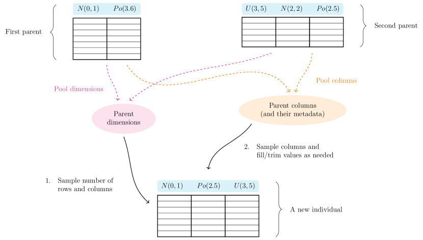
Observe that there is no requirement on the dimensions of the parents to be of similar or equal shapes. This is because the driving aim of the proposed method is to explore the space of all possible datasets. In the case where there is incongruence in the lengths of the two parents, missing values may appear in a shorter column that is sampled. To resolve this, values are sampled from the probability distribution associated with that column to fill in these gaps.

Input: Two parents

Output: An offspring made from the parents ready for mutation

begin

      collate the columns and metadata from each parent in a pool

       sample each dimension from between the parents uniformly

       form an empty dataset with these dimensions

       for each column in the dataset do

            sample a column (and its corresponding metadata) from the pool

             if this column is longer than required then

                  randomly select entries and delete them as needed

             end if

            if this column is shorter than required then

                  sample new values from the metadata and append them to the column as needed

             end if

            add this column to the dataset and record its metadata

            

       end for

      

end

Algorithm 6 The crossover process

2.4 Mutation

Mutation is used in evolutionary algorithms to encourage a broader exploration of the search space at each generation. Under this framework, the mutation process manipulates the phenotype of an individual where numerous things need to be modified including an individual’s dimensions, column metadata and the entries themselves. This process is described in Figure 6.

Figure 6: The stages of the mutation process.

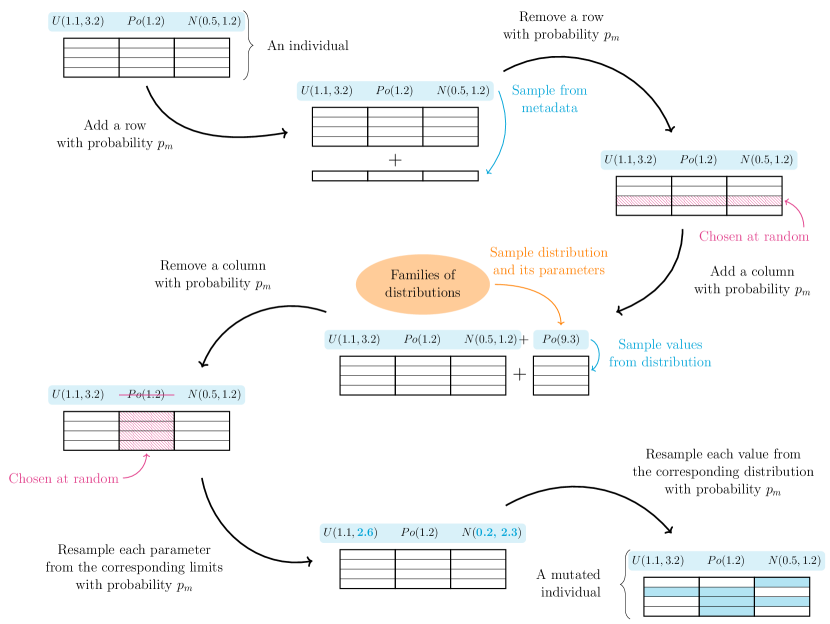
As shown in Figure 6, each of the potential mutations occur with the same probability, $p_{m}$. However, the way in which columns are maintained assure that (assuming appropriate choices for $f$ and $\mathcal{P}$) many mutations in the metadata and the dataset itself will only result in some incremental change in the individual’s fitness relative to, say, a completely new individual.

Input: An individual, $p_{m}$, $R$, $C$, $\mathcal{P}$, $w$

Output: A mutated individual

begin

      sample a random number $r\in[0,1]$

       if $r<p_{m}$ and adding a row would not violate $R$ then

            sample a value from each distribution in the metadata

             append these values as a row to the end of the dataset

            

       end if

      sample a new $r\in[0,1]$

       if $r<p_{m}$ and removing a row would not violate $R$ then

            remove a row at random from the dataset

       end if

      sample a new $r\in[0,1]$

       if $r<p_{m}$ and adding a new column would not violate $C$ then

            create a new column using $\mathcal{P}$ and $w$

             append this column to the end of the dataset

       end if

      sample a new $r\in[0,1]$

       if $r<p_{m}$ and removing a column would not violate $C$ then

            remove a column (and its associated metadata) at random from the dataset

       end if

      for each distribution in the metadata do

            for each parameter of the distribution do

                  sample a random number $r\in[0,1]$

                   if $r<p_{m}$ then

                        sample a new value from within the distribution parameter limits

                         update the parameter value with this new value

                   end if

                  

             end for

            

       end for

      for each entry in the dataset do

            sample a random number $r\in[0,1]$

             if $r<p_{m}$ then

                  sample a new value from the associated column distribution

                   update the entry with this new value

             end if

            

       end for

      

end

Algorithm 7 The mutation process

3 A case study in clustering

3.1 $k$-means clustering

The following examples act as a form of validation for EDO, and also highlight some of the nuances in its use. The objective of these examples is to use the proposed method to reproduce some known results about the clustering of data in the absence of any external forces, and to examine how clustering algorithms are typically evaluated. In particular, the focus will be on the well-known $k$-means (Lloyd’s) algorithm. Clustering was chosen as it is a well-understood problem that is easily accessible - especially when restricted to two dimensions. The $k$-means algorithm is an iterative, centroid-based method that aims to minimise the ‘inertia’ of the current partition, $Z=\left\{Z_{1},\ldots,Z_{k}\right\}$, of some dataset $X$:

$$I(Z,X):=\frac{1}{|X|}\sum_{j=1}^{k}\sum_{x\in Z_{j}}{d(x,z_{j})}^{2}$$ (3)

A full statement of the algorithm to minimise (3) is given in A.1.

This inertia function is taken as the objective of the $k$-means algorithm, and is used for evaluating the final clustering. This is particularly true when the algorithm is not being considered an unsupervised classifier where accuracy may be used [13]. With that, the first example will use this inertia as the fitness function in EDO. That is, to find datasets which minimise $I$.

For the purposes of visualisation, EDO is restricted to the space containing only two-dimensional datasets, i.e. $C=\left((2,2)\right)$. In addition to this, all columns are formed from uniform distributions where the bounds are sampled from the unit interval. Thus, the only family in $\mathcal{P}$ is:

$$\mathcal{U}:=\left\{U(a,b)~{}|~{}a,b\in[0,1]\right\}$$ (4)

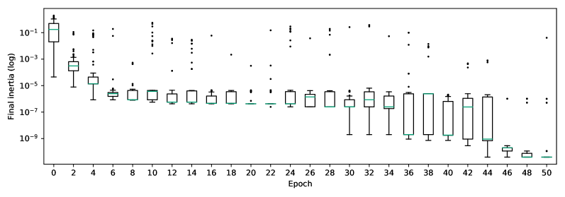
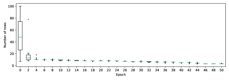
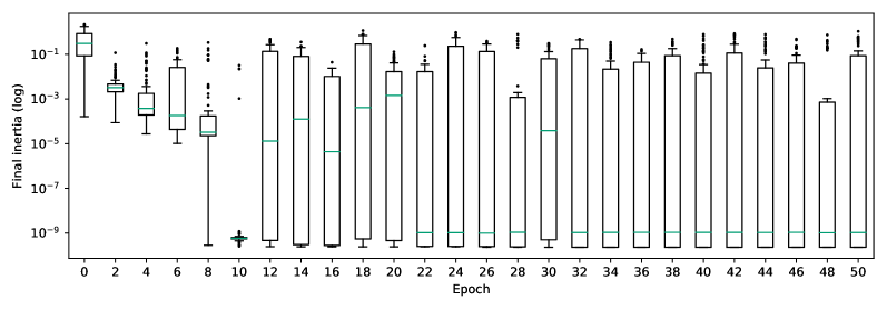
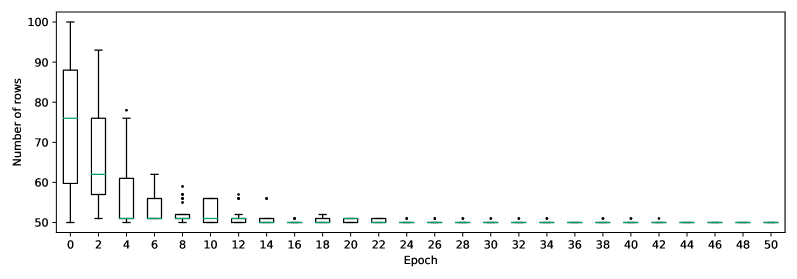
The remaining parameters are as follows: $N~{}=~{}100$, $R~{}=~{}(3,100)$, $M~{}=~{}1000$, $b~{}=~{}0.2$, $l~{}=~{}0$, $p_{m}~{}=~{}0.01$, and shrinkage is excluded. Figure 7 shows an example of the fitness (above) and dimension (below) progression of the evolutionary algorithm under these conditions up until the $50^{th}$ epoch.

There is a steep learning curve here; within the first 50 generations an individual is found with a fitness of roughly $10^{-10}$ which could not be improved on for a further 900 epochs. The same quick convergence is seen in the number of rows. This behaviour is quickly recognised as preferable and was dominant across all the trials conducted in this work. This preference for datasets with fewer rows is expected given that $I$ is the sum of the mean error from each cluster centre. With that, when $k$ is fixed a priori, reducing the number of points in each cluster (i.e. the terms of the second summation) quickly reduces the mean error of that cluster and thus the value of $I$.

Figure 7: Progressions for final inertia and dimension across the first 50 epochs with $R~{}=~{}(3,100)$.

Figure 7: Progressions for final inertia and dimension across the first 50 epochs with $R~{}=~{}(50,100)$.

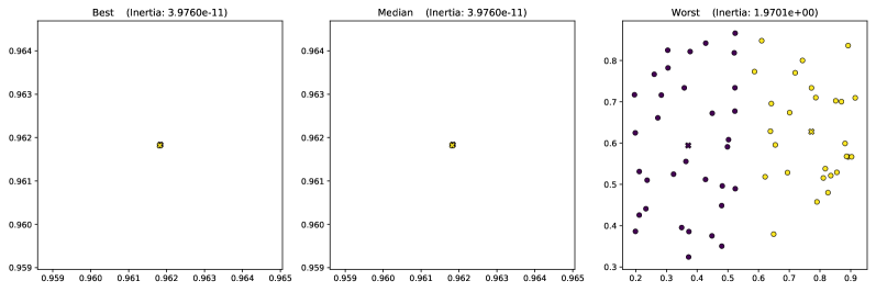
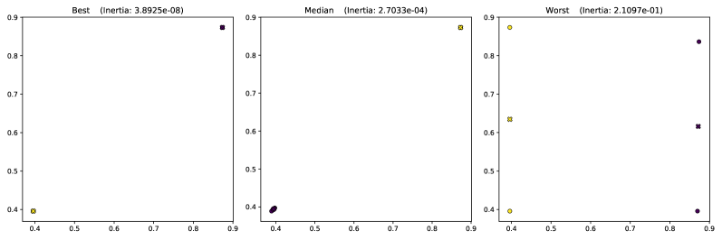
However, something that may be seen as unwanted is a compaction of the cluster centres. Referring to Figure 8a, the best and median individuals show two clusters that are essentially the same point whereas the worst is a random cloud across the whole of $\mathcal{U}$ which was found in the initial population. The kind of behaviour exhibited by the best performing individuals here occurs in part because it is allowed. There are two immediate ways in which this allowed: first, that a near-trivial case is included in $R$ and, secondly, that the fitness function does nothing to penalise the proximity of the inter-cluster means, as well as aiming to reduce the intra-cluster means. This kind of unwanted behaviour highlights a subtlety in how EDO should be used; that experimentation and rigour are required to properly understand an algorithm’s quality.

(a)

(b)

Figure 8: Representative individuals based on inertia with: LABEL:sub@fig:small-inertia-inds $R~{}=~{}(3,100)$; LABEL:sub@fig:large-inertia-inds $R~{}=~{}(50,100)$. Centroids displayed as crosses.

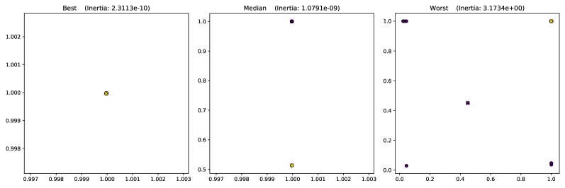
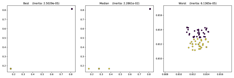
Hence, consider Figure 8b where the individuals have been generated with the same parameters as previously except with adjusted row limits, $R=(50,100)$, so as to exclude this trivial case. In these trials, the results are equivalent: the worst performing individuals are without structure whilst the best-performing individuals display clusters that are dense about a single point despite the minimum number of rows being increased. Supposing this was not already a known result, we can see mounting evidence in favour of this compaction being ‘optimal’ behaviour in a dataset for $k$-means clustering.

However, the fitness function may be addressed still, and more extensive studying may be done. Indeed, the final inertia could be considered a flawed or fragile fitness function if it is supposed to evaluate the efficacy of the $k$-means algorithm. Incorporating the inter-cluster spread to the fitness of an individual dataset would reduce this observed compaction. For instance, the silhouette coefficient is a metric used to evaluate the appropriateness of a clustering to a dataset and does precisely that. The silhouette coefficient of a clustering of a dataset is given by the mean of the silhouette value, $S(x)$, of each point $x\in Z_{j}$ in each cluster:

$$\begin{gathered}A(x):=\frac{1}{|Z_{j}|-1}\sum_{y\in Z_{j}\setminus\{x\}}d(x,y),\\ B(x):=\min_{k\neq j}\frac{1}{|Z_{k}|}\sum_{w\in Z_{k}}d(x,w),\\ S(x):=\begin{cases}\frac{B(x)-A(x)}{\max\left\{A(x),B(x)\right\}}&\quad\text{if }|Z_{j}|>1\\ 0&\quad\text{otherwise}\end{cases}\end{gathered}$$ (5)

The optimisation of the silhouette coefficient is analogous to finding a dataset which increases both the intra-cluster cohesion (the inverse of $A$) and inter-cluster separation ($B$). Hence, the objective of minimising inertia is addressed by maximising cohesion. Meanwhile, the additional desire to spread out the clusters is considered by maximising separation.

Repeating the trials with the same parameters as with inertia, the silhouette fitness function yields the results summarised in Figures 9 and 9. Irrespective of row limits, the datasets produced show increased separation from one another whilst maintaining low values in the final inertia of the clustering as shown in Figure 10. Again, the form of the individual clusters is much the same. The low values of inertia correspond to tight clusters, and the tightest clusters are those with a minimal number of points, i.e. a single point. As with the previous example, albeit at a much slower rate, the preferable individuals are those leading toward this case. That this gradual reduction in the dimension of the individuals occurs despite adjusting the fitness function and considering the space which excludes the trivial case bolsters the claim that the base case is also optimal.

At this point, it should be noted that, due to the nature of the implementation, any individual from any generation may be retrieved and studied should the final results be too concentrated on any given case. The summary provided here is one particular way of studying the body of datasets generated with this method and this transparency in the history and progression of the proposed method is something that sets it apart from other methods such as GANs which have a reputation of providing so-called ‘black box’ solutions.

Figure 9: Progressions for silhouette and dimension across 1000 epochs at 100 epoch intervals with $R~{}=~{}(3,100)$.

Figure 9: Progressions for silhouette and dimension across 1000 epochs at 100 epoch intervals with $R~{}=~{}(50,100)$.

(a)

(b)

Figure 10: Representative individuals based on silhouette with: LABEL:sub@fig:small-silhouette-inds $R~{}=~{}(3,100)$; LABEL:sub@fig:large-silhouette-inds $R~{}=~{}(50,100)$. Centroids displayed as crosses.

3.2 Comparison with DBSCAN

The extent of the capabilities EDO holds as a tool to better understand an algorithm are especially apparent when comparing an algorithm against another (or set of others) simultaneously. This is done by utilising the freedom of choice in a fitness function for EDO. Consider two algorithms, $A$ and $B$, and some common metric between them, $g$. Then their similarities and contrasts can be explored by considering the differences in this metric on the two algorithms. In terms of EDO, this means using $f=g_{A}-g_{B}$, $f=g_{B}-g_{A}$ or $f=\left|g_{B}-g_{A}\right|$ as the fitness function. By doing so, pitfalls, edge cases or fundamental conditions for the method may be highlighted. Overall, this process allows the researcher to more deeply learn about the method of interest beyond the traditional method of literature comparison on a particular example.

Consider the following use case with another clustering algorithm of a different form, Density Based Spatial Clustering of Applications with Noise (DBSCAN). In this particular case, the objective is to find datasets for which the method of interest, $k$-means, outperforms its alternative, DBSCAN. Here there is no concept of inertia as DBSCAN is density-based and is able to identify outliers [11]. As such, a valid metric must be chosen. One such metric is the silhouette score as defined in (5).

In this case, however, an adjustment to the fitness function must be made so as to accommodate for the condition of the silhouette coefficient that there must be more than one cluster present. Let $S_{k}(X)$ and $S_{D}(X)$ denote the silhouette coefficients of the clustering found by $k$-means and DBSCAN respectively. Then the fitness function is defined to be:

$$f(X)=\begin{cases}S_{D}(X)-S_{k}(X),&\quad\text{\begin{tabular}[]{l}if DBSCAN identifies two or\\ more clusters (inc.\ noise)\end{tabular} }\\ \infty&\quad\ \ \text{otherwise.}\end{cases}$$ (6)

There are several remarks to be made here. First, note the order of the subtraction here as EDO minimises fitness functions by default. Also, $f$ takes values in the range $[-2,2]$ where $-2$ is the best, i.e. $S_{D}(X)=-1$ and $S_{k}(X)=1$. Likewise, 2 is the worst score. Finally, the silhouette coefficient requires at least two clusters to be present and so if DBSCAN identifies a single cluster then that individual will be penalised heavily under this fitness function when, in fact, that clustering may be of high quality. As such, this fitness function may require adjustment.

It must also be acknowledged that $k$-means and DBSCAN share no common parameters and so direct comparison is more difficult. For the purposes of this example, only one set of parameters is used but a thorough investigation should include a parameter sweep in similar, real-world use cases. The parameters being used are $k~{}=~{}3$ for $k$-means, and $\epsilon~{}=~{}0.1,\ MinPoints~{}=~{}5$ for DBSCAN. This set was chosen following informal experimentation using the Python library Scikit-learn [27] to find comparable parameters in the given search space defined by the EDO parameters used previously with $R~{}=~{}(50,100)$.

Figure 11: Progressions for difference in silhouette ($k$-means-preferable) and dimension across 1000 epochs at 100 epoch intervals.

(a)

(b)

Figure 12: Representative individuals from a $k$-means-preferable run with clustering by: LABEL:sub@fig:dbscan-inds-k $k$-means; LABEL:sub@fig:dbscan-inds-d DBSCAN. Concave and convex hulls illustrated by shading and outline respectively.

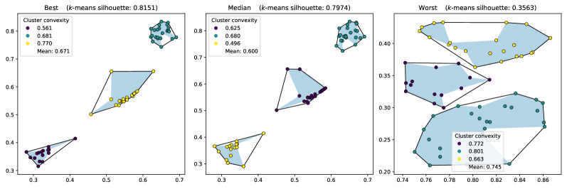
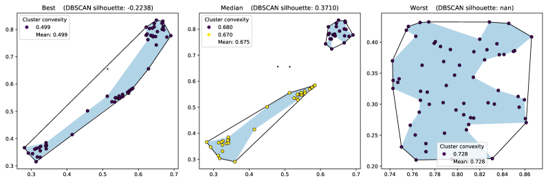
Figure 11 shows a summary of the progression of EDO for this use case. As with the previous examples where $R~{}=~{}(50,100)$, the variation in the population fitness is unstable but there is a clear trend of improvement in the best individual over the course of the run. There is also a convergence seen in the number of rows a dataset has. The resting dimension varied across the trials conducted in this work but none exhibited a dramatic shift toward the lower limit of 50 rows as with previous examples. This is suggestive of a more competitive environment for individuals where slight changes to an individual can drastically alter their fitness.

The effect of such changes can be seen in Figure 12 where representative individuals are shown for this example. Here, the best performing individual, when clustered by $k$-means, shows three clear and nicely separated clusters. Note that they are not so tightly packed; again, this suggests that the route to an optimal individual is less clearly defined. In contrast, when the same dataset is clustered by DBSCAN a single cluster is found with a single noise point held within the convex hull of the cluster, i.e. there are overlapping clusters (since noise points form a single cluster). Hence, along with the fact that the larger cluster is widely spread, it follows that the clustering has a relatively small, negative silhouette coefficient.

Another point of interest here is the convexity of the clusters. A known condition for the success of $k$-means is that the presented clusters are of roughly equal size and are convex. This is due to the overall objective being to approximate the centroidal Voronoi tessellation [9]. Without this condition, up to the correct choice of $k$, the algorithm will fail to produce adequate results for either inertia or silhouette. DBSCAN, on the other hand, does not have this condition and is able to detect non-convex clusters so long as they are dense enough. Figure 12 shows the clustering found by each method and the respective convex and concave hulls of the clusters found. The ‘concave hull’ of a cluster is taken to be the $\alpha$-shape of the cluster’s data points [10] where $\alpha$ is determined to be the smallest value such that all the points in the cluster are contained in a single polygon. The convexity of cluster $Z_{j}$, denoted $\mathcal{C}_{j}$, is then determined to be the ratio of the area of its concave hull, $H_{c}$, to the area of its convex hull, $H_{v}$ [30]:

$$\mathcal{C}_{j}:=\frac{area(H_{c})}{area(H_{v})}$$ (7)

With this definition, it should be clear that a perfectly convex cluster, such as a single point or line, would have $\mathcal{C}_{j}=1$.

It can be seen that the convexity of the clustering found by $k$-means appears to be higher than that by DBSCAN. This was apparent across all trials conducted in this work and indicates that the condition for convex clusters is being sought out during the optimisation process. Meanwhile, however, it is not clear whether the performance of DBSCAN falls owing to its parameters or the method itself. This is a point where parameter sweeping would prove most useful so as to determine a crossing point for these two driving forces.

Now, to add to the discussion above, the inverse optimisation should be considered. That is, using the same parameters, the datasets for which DBSCAN outperforms $k$-means with respect to the silhouette coefficient are to be investigated. This is equivalent to using $-f$ as the fitness function except with the same penalty of $\infty$ for the case set out in (6).

Figure 13: Progressions for difference in silhouette (DBSCAN-preferable) and dimension across 1000 epochs at 100 epoch intervals.

(a)

(b)

Figure 14: Representative individuals from a DBSCAN-preferable run with clustering by: LABEL:sub@fig:dbscan-inds-k $k$-means; LABEL:sub@fig:dbscan-inds-d DBSCAN. Concave and convex hulls illustrated by shading and outline respectively.

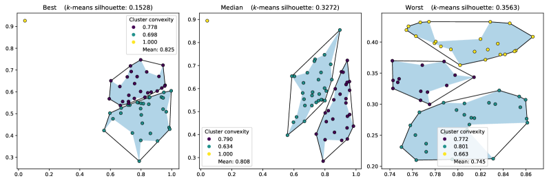
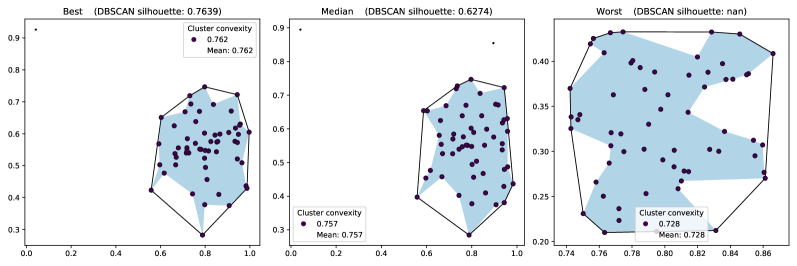
Figures 13 and 14 show the same summary as above with the revised fitness function. Inspecting the former, it is seen that the best fitness found is worse than with the previous example. This, in part, is due to the fact that $k$-means cannot find a clustering with negative values as no clusters may overlap. It can, however, produce results with small silhouette scores where the clusters are tightly packed. Hence, the best fitness score is now $-1$ whereas the worst is 2, still.

Note in the first two frames of Figure 14a how $k$-means is forced to split what is evidently a single cluster in two whereas DBSCAN is able to identify the single cluster and the outlying noise (Figure 14b). The proximity of these clusters has then dragged the silhouette score down for $k$-means. Referring to Figure 14b, this kind of behaviour is certainly preferable for DBSCAN under these parameters: the beginning individuals are likely random clouds (as seen in the rightmost two frames of the figure) and the simplest step toward a fit dataset is one that maintains that vaguely dense body with minimal noise points far from it.

As has already been stated, the software implementation of the EDO method has been produced in line with the best practices of open source software development and reproducible research. In aid of this, all of the source code used in these examples (including to create the figures) has been archived under the DOI 10.5281/zenodo.3492236. Likewise, all of the data produced to support this case study have been archived under the DOI 10.5281/zenodo.3492228.

4 Conclusion

In this paper we have introduced a novel approach to understanding the quality of an algorithm by exploring the space in which their well-performing datasets exist. Following a detailed explanation of its internal mechanisms, a case study in $k$-means clustering was offered as validation for the proposed method. The method was able to reveal some known results without prior knowledge when investigating $k$-means in several scenarios, and again when comparing $k$-means and another leading clustering method, DBSCAN.

The method itself utilises biological operators to traverse a potentially broad region of the space of all possible datasets. This is done in an organic way with a minimal external framework attached. The generative nature of the proposed method also provides transparency and richness to the solution when compared to other contemporary techniques for artificial data generation as the entire history of individuals is preserved. While other search and optimisation methods exist, the decision to use an EA here was down to this transparency and the ease with which to implement biological operators that are both meaningful and easily understood.

The Evolutionary Dataset Optimisation method is dependent on a number of parameters set out in this work one of which is the choice of distribution families, $\mathcal{P}$; these families go on to define the general statistical shape of the columns of the datasets that are produced and also control the present data types. The relationship between columns and their associated distribution is not causal and appropriate methods should be employed to understand the structure and characteristics of the data produced before formal conclusions are made as set out in the case study provided.

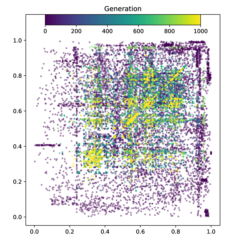
It is known that EAs might terminate at a local optimum and may not be able to traverse the entire sample space [35], or even a sufficient part of it. This would be even more problematic in the case presented in this work where the sample space is not even of a fixed size or data type. In all experiments carried out for this work, this theoretic limitation has not arisen. Figure 15 shows an exploration of the sample space and it is evident that the EDO method was able to explore a large proportion of it. In the early stages, it is also clear here how the EA got stuck in small parts of the search space before later moving toward a subregion of the unit square.

Figure 15: A scatter of all the individuals found at 50 epoch intervals in the first example of Section 3.2, i.e. those summarised in Figure 12.

Although this does provide evidence to say that the EA’s current design can sufficiently explore its given search space, it does not provide any guarantee that this will happen, even in expectation. Proving this theoretically is an area for further investigation.

Something that does stand against EAs is their tendancy to find the ‘easy’ way out. That is, reducing down to the simplest solution which solves the given problem. In most cases, that is not a problem and is often, in fact, favourable. Throughout the case study provided, this is seen to happen. Figure 15 shows this behaviour again by the strong diagonal region in later generations. In that particular example, the easiest solution for the EA (i.e. for $k$-means to outperform DBSCAN) was to collapse one dimension of the search space to make the problem one-dimensional. This kind of behaviour is not necessarily a bad thing as trivial, basic and simple cases are of great importance when understanding an algorithm’s quality.

However, should that be a problem, then the objective function could be adjusted accordingly. In the case study, several iterations of fitness functions were examined but each was adjusted by hand according to what was apparent at the time. Due to the architecture of the implementation of this method, this could be done in practicality. For instance, a similar strategy could be employed automatically by a more sophisticated fitness function that retains some information about the datasets generated from previous runs of EDO on a particular (or at least similar) parameter set. In this way, the currently completely unsupervised learning conducted by the EA could be ushered away from less helpful solutions (via some penalty, say) and toward previously unexplored behaviours. This automatic, iterative application of the proposed method would likely reveal more sophisticated insights into a particular algorithm.

In essence, the proposed method is merely a tool that demonstrates the benefit of the flipped paradigm set out in this work. The concept of where ‘good’ datasets exist is not something that is well-documented in literature and the hope of this work is that Evolutionary Dataset Optimisation acts as a starting point for further works to come.

Conflict of interest

The authors declare that they have no conflict of interest.

Appendix A Appendix

A.1 Lloyd’s algorithm

Input: a dataset $X$, a number of centroids $k$, a distance metric $d$

Output: a partition of $X$ into $k$ parts, $Z$

begin

      select $k$ initial centroids, $z_{1},\ldots,z_{k}\in X$

       while any point changes cluster or some stopping criterion is not met do

            assign each point, $x\in X$, to cluster $Z_{j^{*}}$ where:

$$j^{*}=\operatorname*{arg\,min}_{j=1,\ldots,k}\left\{{d\left(x,z_{j}\right)}^{2}\right\}$$

             recalculate all centroids by taking the intra-cluster mean:

$$z_{j}=\frac{1}{|Z_{j}|}\sum_{x\in Z_{j}}x$$

       end while

      

end

Algorithm 8 $k$-means (Lloyd’s)

A.2 Implementation example

Below is an example of how the Python implementation was used to complete the first example, including the definition of the fitness function.

⬇

import edo

from edo.pdfs import Uniform

from sklearn.cluster import KMeans

def fitness(dataframe, seed):

"""␣Return␣the␣final␣inertia␣of␣2-means␣on␣the␣‘dataframe‘

␣␣␣␣for␣the␣given␣‘seed‘.␣"""

km = KMeans(n_clusters=2, random_state=seed).fit(dataframe)

return km.inertia_

Uniform.param_limits["bounds"] = [0, 1]

pop_history, fit_history = edo.run_algorithm(

fitness, size=100, row_limits=[3, 100], col_limits=[2, 2],

families=[Uniform], max_iter=1000, best_prop=0.2,

mutation_prob=0.01, seed=0, root="out",

fitness_kwargs={"seed": 0},

)

References

- [1] Abualigah, L.M., Khader, A.T., Hanandeh, E.S.: A combination of objective functions and hybrid krill herd algorithm for text document clustering analysis. Engineering Applications of Artificial Intelligence 73(Int. J. Comput. Sci. Eng. Appl. 5 1 2015), 111–125 (2018). DOI 10.1016/j.engappai.2018.05.003
- [2] Abualigah, L.M., Khader, A.T., Hanandeh, E.S.: Hybrid clustering analysis using improved krill herd algorithm. Applied Intelligence 48(11), 4047–4071 (2018). DOI 10.1007/s10489-018-1190-6
- [3] Amirjanov, A.: Modeling the dynamics of a changing range genetic algorithm. Procedia Computer Science 102, 570 – 577 (2016). DOI https://doi.org/10.1016/j.procs.2016.09.444
- [4] Bäck, T.: Selective pressure in evolutionary algorithms: a characterization of selection mechanisms. In: Proceedings of the First IEEE Conference on Evolutionary Computation. IEEE World Congress on Computational Intelligence, pp. 57–62 (1994). DOI 10.1109/ICEC.1994.350042
- [5] Campos, G., Zimek, A., Sander, J., Campello, R., Micenková, B., Schubert, E., Assent, I., Houle, M.: On the evaluation of unsupervised outlier detection: measures, datasets, and an empirical study. Data Mining and Knowledge Discovery 30(4), 891–927 (2016). DOI 10.1007/s10618-015-0444-8
- [6] Chen, Y., Elliot, M., Sakshaug, J.: A genetic algorithm approach to synthetic data production. In: PrAISe@ECAI (2016)
- [7] Chen, Y., Elliot, M., Smith, D.: The application of genetic algorithms to data synthesis: A comparison of three crossover methods. In: Privacy in Statistical Databases, pp. 160–171. Springer International Publishing (2018). DOI 10.1007/978-3-319-99771-1˙11
- [8] Dau, H.A., Keogh, E., Kamgar, K., Yeh, C.C.M., Zhu, Y., Gharghabi, S., Ratanamahatana, C.A., Yanping, Hu, B., Begum, N., Bagnall, A., Mueen, A., Batista, G., Hexagon-ML: The UCR time series classification archive (2018). https://www.cs.ucr.edu/~eamonn/time_series_data_2018/
- [9] Du, Q., Emelianenko, M., Ju, L.: Convergence of the lloyd algorithm for computing centroidal voronoi tessellations. SIAM Journal on Numerical Analysis 44(1), 102–119 (2006). DOI 10.1137/040617364
- [10] Edelsbrunner, H., Kirkpatrick, D., Seidel, R.: On the shape of a set of points in the plane. IEEE Transactions on Information Theory 29(4), 551–559 (1983). DOI 10.1109/TIT.1983.1056714
- [11] Ester, M., Kriegel, H.P., Sander, J., Xu, X.: A density-based algorithm for discovering clusters in large spatial databases with noise. In: KDD (1996)
- [12] Goodfellow, I., Pouget-Abadie, J., Mirza, M., Xu, B., Warde-Farley, D., Ozair, S., Courville, A., Bengio, Y.: Generative adversarial nets. In: Advances in Neural Information Processing Systems 27, pp. 2672–2680. Curran Associates, Inc. (2014). URL http://papers.nips.cc/paper/5423-generative-adversarial-nets.pdf
- [13] Huang, Z.: Extensions to the k-means algorithm for clustering large data sets with categorical values. Data Mining and Knowledge Discovery 2(3), 283–304 (1998). DOI 10.1023/A:1009769707641
- [14] Jebari, K.: Selection methods for genetic algorithms. International Journal of Emerging Sciences 3, 333–344 (2013)
- [15] Jiménez, R.C., Kuzak, M., Alhamdoosh, M., Barker, M., Batut, B., Borg, M., Capella-Gutierrez, S., Chue Hong, N., Cook, M., Corpas, M., Flannery, M., Garcia, L., Gelpí, J.L., Gladman, S., Goble, C., González Ferreiro, M., Gonzalez-Beltran, A., Griffin, P.C., Grüning, B., Hagberg, J., Holub, P., Hooft, R., Ison, J., Katz, D.S., Leskošek, B., López Gómez, F., Oliveira, L.J., Mellor, D., Mosbergen, R., Mulder, N., Perez-Riverol, Y., Pergl, R., Pichler, H., Pope, B., Sanz, F., Schneider, M.V., Stodden, V., Suchecki, R., SvobodováVařeková, R., Talvik, H.A., Todorov, I., Treloar, A., Tyagi, S., van Gompel, M., Vaughan, D., Via, A., Wang, X., Watson-Haigh, N.S., Crouch, S.: Four simple recommendations to encourage best practices in research software. F1000Research 6, ELIXIR–876 (2017). DOI 10.12688/f1000research.11407.1
- [16] Koleejan, C., Xue, B., Zhang, M.: Code coverage optimisation in genetic algorithms and particle swarm optimisation for automatic software test data generation. 2015 IEEE Congress on Evolutionary Computation (CEC) pp. 1204–1211 (2015)
- [17] Kuehn, M., Severin, T., Salzwedel, H.: Variable mutation rate at genetic algorithms: Introduction of chromosome fitness in connection with multi-chromosome representation. International Journal of Computer Applications 72, 31–38 (2013). DOI 10.5120/12636-9343
- [18] Leung, Y.W., Wang, Y.: An orthogonal genetic algorithm with quantization for global numerical optimization. IEEE Transactions on Evolutionary Computation 5(1), 41–53 (2001). DOI 10.1109/4235.910464
- [19] Liu, L., Cheng, L., Liu, Y., Jia, Y., Rosenblum, D.: Recognizing complex activities by a probabilistic interval-based model (2016)
- [20] Martí, L., García, J., Berlanga, A., Molina, J.M.: A stopping criterion for multi-objective optimization evolutionary algorithms. Information Sciences 367-368, 700 – 718 (2016). DOI https://doi.org/10.1016/j.ins.2016.07.025
- [21] Matejka, J., Fitzmaurice, G.: Same stats, different graphs: Generating datasets with varied appearance and identical statistics through simulated annealing. In: Proceedings of the 2017 CHI Conference on Human Factors in Computing Systems, CHI ’17, pp. 1290–1294. ACM (2017). DOI 10.1145/3025453.3025912
- [22] McKinney, W.: Data structures for statistical computing in python. Proceedings of the 9th Python in Science Conference (2010–). URL https://pandas.pydata.org/. [Online; accessed 2019-03-01]
- [23] Michael, C.C., McGraw, G., Schatz, M.: Generating software test data by evolution. IEEE Trans. Software Eng. 27, 1085–1110 (2001)
- [24] Motoki, T.: Calculating the expected loss of diversity of selection schemes. Evolutionary Computation 10(4), 397–422 (2002). DOI 10.1162/106365602760972776
- [25] Oliphant, T.: NumPy: A guide to NumPy. USA: Trelgol Publishing (2006–). URL http://www.numpy.org/. [Online; accessed 2019-03-01]
- [26] Olson, R.S., La Cava, W., Orzechowski, P., Urbanowicz, R.J., Moore, J.H.: PMLB: a large benchmark suite for machine learning evaluation and comparison. BioData Mining 10(1), 36 (2017). DOI 10.1186/s13040-017-0154-4
- [27] Pedregosa, F., Varoquaux, G., Gramfort, A., Michel, V., Thirion, B., Grisel, O., Blondel, M., Prettenhofer, P., Weiss, R., Dubourg, V., Vanderplas, J., Passos, A., Cournapeau, D., Brucher, M., Perrot, M., Duchesnay, E.: Scikit-learn: Machine Learning in Python . Journal of Machine Learning Research 12, 2825–2830 (2011)
- [28] Semenkin, E., Semenkina, M.: Self-configuring genetic algorithm with modified uniform crossover operator. In: Advances in Swarm Intelligence, pp. 414–421 (2012)
- [29] Sharifipour, H., Shakeri, M., Haghighi, H.: Structural test data generation using a memetic ant colony optimization based on evolution strategies. Swarm and Evolutionary Computation 40, 76 – 91 (2018). DOI https://doi.org/10.1016/j.swevo.2017.12.009
- [30] Sonka, M., Hlavac, V., Boyle, R.: Image Processing, Analysis and Machine Vision. Springer US (1993). DOI 10.1007/978-1-4899-3216-7
- [31] Suganuma, M., Shirakawa, S., Nagao, T.: A genetic programming approach to designing convolutional neural network architectures. In: GECCO (2017)
- [32] Sun, Y., Xue, B., Zhang, M., Yen, G.G.: Automatically designing CNN architectures using genetic algorithm for image classification. CoRR abs/1808.03818 (2018)
- [33] The EDO library developers: EDO: v0.2.1 (2019). DOI 10.5281/zenodo.2651075. URL http://dx.doi.org/10.5281/zenodo.2651075
- [34] Torralba, A., Efros, A.A.: Unbiased look at dataset bias. Proceedings of the 2011 IEEE Conference on Computer Vision and Pattern Recognition (2011). DOI 10.1109/CVPR.2011.5995347. URL http://dx.doi.org/10.1109/CVPR.2011.5995347
- [35] Vikhar, P.A.: Evolutionary algorithms: A critical review and its future prospects. In: 2016 International Conference on Global Trends in Signal Processing, Information Computing and Communication (ICGTSPICC), pp. 261–265 (2016). DOI 10.1109/ICGTSPICC.2016.7955308
- [36] Wang, N., Shi, J., Yeung, D.Y., Jia, J.: Understanding and diagnosing visual tracking systems (2015). DOI 10.1109/ICCV.2015.355
- [37] Wu, X., Wu, X., Kumar, V.: The Top Ten Algorithms in Data Mining. CRC (2009)
- [38] Zhao, W., Ma, H., He, Q.: Parallel k-means clustering based on MapReduce. In: Cloud Computing, pp. 674–679. Springer Berlin Heidelberg (2009). DOI 10.1007/978-3-642-10665-1˙71