Linear response for macroscopic observables in high-dimensional systems

Abstract

The long-term average response of observables of chaotic systems to dynamical perturbations can often be predicted using linear response theory, but not all chaotic systems possess a linear response. Macroscopic observables of complex dissipative chaotic systems, however, are widely assumed to have a linear response even if the microscopic variables do not, but the mechanism for this is not well-understood.

We present a comprehensive picture for the linear response of macroscopic observables in high-dimensional coupled deterministic dynamical systems, where the coupling is via a mean field and the microscopic subsystems may or may not obey linear response theory. We derive stochastic reductions of the dynamics of these observables from statistics of the microscopic system, and provide conditions for linear response theory to hold in finite dimensional systems and in the thermodynamic limit. In particular, we show that for large systems of finite size, linear response is induced via self-generated noise.

We present examples in the thermodynamic limit where the macroscopic observable satisfies LRT, although the microscopic subsystems individually violate LRT, as well a converse example where the macroscopic observable does not satisfy LRT despite all microscopic subsystems satisfying LRT when uncoupled. This latter, maybe surprising, example is associated with emergent non-trivial dynamics of the macroscopic observable. We provide numerical evidence for our results on linear response as well as some analytical intuition.

Since its introduction mid-last century, linear response theory (LRT) has been a cornerstone of statistical mechanics. If a system has a linear response, one can estimate the change of expectation values caused by a perturbation of a parameter using only information of the unperturbed system. LRT has been successfully applied in numerous areas, ranging from neurophysiology to climate science. It is widely believed that high-dimensional complex dynamical systems satisfy LRT, largely based on successes in applications. Separate efforts by mathematicians to understand the dynamical underpinnings of linear response theory, however, have found that many low-dimensional systems such as the logistic map do not obey LRT, but instead exhibit a rough dependency of their statistical properties with respect to perturbations. In this work we investigate the conditions for and mechanisms by which a system comprised of low-dimensional subunits—which individually may or may not obey LRT—may at a macroscopic scale have a linear response.

I Introduction

Since its introduction in the 1960s, linear response theory (LRT) has been widely used across numerous disciplines to quantify the change of the mean behaviour of observables in a perturbed environment. LRT is valid, in essence, provided the invariant measure varies differentiably with respect to the perturbation; consequently LRT allows for a Taylor expansion of the perturbed invariant measure around the unperturbed invariant measure. Hence, when valid, LRT provides an expression of the average of some observable when subjected to small perturbations from an unperturbed state – the system’s so called response – entirely in terms of statistical information from the unperturbed system.

Climate scientists in particular have successfully applied LRT to eke out valuable information about the change of certain atmospheric and oceanic observables under changed climatic conditions. Applications include atmospheric toy models Majda, Abramov, and Gershgorin (2010); Lucarini and Sarno (2011); Abramov and Majda (2007, 2008); Cooper and Haynes (2011); Cooper, Esler, and Haynes (2013), barotropic models Bell (1980); Gritsun and Dymnikov (1999); Abramov and Majda (2009), quasi-geostrophic models Dymnikov and Gritsoun (2001), atmospheric models North, Bell, and Hardin (1993); Cionni, Visconti, and Sassi (2004); Gritsun, Branstator, and Dymnikov (2002); Gritsun and Branstator (2007); Gritsun, Branstator, and Majda (2008); Ring and Plumb (2008); Gritsun (2010) and coupled climate models Langen and Alexeev (2005); Kirk-Davidoff (2009); Fuchs, Sherwood, and Hernandez (2014); Ragone, Lucarini, and Lunkeit (2016). The seminal work by Ruelle Ruelle (1997, 1998, 2009a, 2009b) rigorously established that LRT is valid in uniformly hyperbolic Axiom A systems. Success in reliably estimating the response of a physical system, as exemplified by the above applications in the climate sciences, prompted scientists to believe that general chaotic dynamical systems obeyed LRT. This belief was proven wrong by Baladi and co-workers Baladi and Smania (2008, 2010); Baladi (2014); Baladi, Benedicks, and Schnellmann (2015); De Lima and Smania (2018) who showed that simple dynamical systems such as the logistic map violate LRT and support an invariant measure that changes non-smoothly with respect to the perturbation. This raises the question of how a high-dimensional dynamical system, despite its constituent subsystems typically individually violating LRT, may exhibit linear response.

The majority of the scientific community, including the authors, believe that the interaction between the microscopic constituents in typical high-dimensional systems leads to an emergence of LRT at the macroscopic level. How exactly this is achieved and what the conditions are for the dynamical systems for which LRT is guaranteed, however, remains an open question. In the literature the validity of LRT in high-dimensional deterministic systems is often justified by appealing to the chaotic hypothesis of Gallavotti and Cohen Gallavotti and Cohen (1995a, b); Gallavotti (2019) according to which the attracting dynamics of high-dimensional system behaves for all practical purposes as an Anosov system. However, even under this hypothesis one cannot relate the equivalent Anosov systems for different perturbations, which is the focus of LRT. In particular, for dissipative systems the response of the attracting dynamics to perturbations depends on the properties of the flow outside the attractor as well as on it: off the attractor the flow may be non-hyperbolic, and hence leading to a breakdown of linear response. In stochastic systems, however, it is well established that LRT can be justified Hänggi (1978); Hairer and Majda (2010).

In previous work, we argued that a combination of statistical limits of the high-dimensional system and a sufficient degree of heterogeneity in the system causes a high-dimensional system to obey LRT, even when the individual microscopic subsystems do not obey LRT Wormell and Gottwald (2018). We considered a single resolved degree of freedom weakly coupled to $M$ unresolved uncoupled degrees of freedom, the so called heat bath, which evolve according to their own randomly drawn parameters. Both the distinguished degree of freedom as well as the heat bath were described by logistic maps, which individually violate LRT. In the thermodynamic limit we derived a stochastic limit system for the distinguished degree of freedom; it was shown, however, that the mere presence of stochasticity is not sufficient to guarantee LRT, but the microscopic subsystems need to be appropriately heterogeneous, with the parameters of the logistic map drawn from a sufficiently smooth distribution. The perturbations considered were homogeneous perturbations of the randomly-drawn logistic parameters in the microscopic heat bath system as well as general smooth perturbations in the evolution of the distinguished macroscopic variable.

We continue this line of research and consider here macroscopic observables of high-dimensional dynamical systems whose microscopic constituents may violate LRT, rather than observables only of individual distinguished degrees of freedom. We extend our previous work to consider more general perturbations than homogeneously perturbing the parameters, and include the more realistic case when the microscopic dynamics are globally coupled via a mean field. This latter case has been well-studied, particularly in the case where the coupling is strictly attractive, and complex emergent dynamics at the level of the mean-field have been observedKaneko (1990); Shibata, Chawanya, and Kaneko (1999); Pikovsky and Kurths (1994); Ershov and Potapov (1995, 1997); Sélley and Bálint (2016). We shall provide a systematic macroscopic reduction for the mean-field coupled dynamics, which we use to study a range of interesting dynamical scenarios in the context of linear response. We provide a comprehensive picture of the linear response behaviour of macroscopic observables, for uncoupled and for mean field coupled systems, and we find that the existence of LRT depends in an intricate way on the combination of effective stochastic behaviour of the macroscopic observable, the macroscopic dynamics of the thermodynamic limit, and on the smoothing property of heterogeneously distributed dynamical parameters of the microscopic subsystems. Indeed, we will present a case when all individual microscopic subsystems obey LRT when uncoupled, but the collective macroscopic dynamics violates LRT, and cases where this holds vice versa. To corroborate our findings, we will use a recently developed statistical test which allows to probe for the validity of LRT in a given time series Gottwald, Wormell, and Wouters (2016).

The paper is organized as follows. Section II briefly reviews LRT. We introduce the high-dimensional systems under consideration in Section III and summarise our results in Section IV. Sections V and VI provide numerical evidence and an analytical treatment corroborating the results summarized in Table 1 for uncoupled and for mean field coupled systems. We conclude with a discussion and an outlook in Section VII.

II Linear response theory

We briefly review some basic notation of linear response theory. Consider a family of dynamical systems $f_{\varepsilon}:D\to D$ on some space $D$ where the map $f_{\varepsilon}$ depends smoothly on the parameter $\varepsilon$ and where for each $\varepsilon$ the dynamical system admits a unique invariant physical measure $\mu_{\varepsilon}$. An ergodic measure is called physical if for a set of initial conditions of nonzero Lebesgue measure the temporal average of a typical observable converges to the spatial average over this measure. LRT is concerned with the change of the average of an observable $\phi:D\to{\mathbb{R}}$,

$$\mathbb{E}^{\varepsilon}[\phi]=\int_{D}\phi\,d\mu_{\varepsilon}$$

upon varying $\varepsilon$. A system exhibits linear response at $\varepsilon=\varepsilon_{0}$, if the derivative

$$\mathbb{E}^{\varepsilon_{0}}[\phi]^{\prime}:=\frac{\partial}{\partial\varepsilon}\mathbb{E}^{\varepsilon}[\phi]_{|_{\varepsilon_{0}}}$$

exists. A sufficient condition for this is that the invariant measure $\mu_{\varepsilon}$ is differentiable with respect to $\varepsilon$. This derivative can be expressed entirely in terms of the invariant measure $\mu_{\varepsilon_{0}}$ of the unperturbed system using so-called linear response formulae Ruelle (2009a, 1998); Baladi (2014). The average of an observable of the perturbed state is then expressed to first order as

$$\mathbb{E}^{\varepsilon}[\phi]\approx\mathbb{E}^{\varepsilon_{0}}[\phi]+(\varepsilon-\varepsilon_{0})\,\mathbb{E}^{\varepsilon_{0}}[\phi]^{\prime}.$$

If the derivative exists, then this expansion expresses the remarkable result that the average of the perturbed state is determined up to $o(\varepsilon-\varepsilon_{0})$ by the properties of the unperturbed system. If however it does not exist, we say there is a breakdown of linear response, which manifests itself in a rough dependency of averages of the observable on the perturbation $\varepsilon$ Gottwald, Wormell, and Wouters (2016).

III Model

Figure 1: General set-up. We consider the behaviour of macroscopic observables $\Psi$ which are constructed either from (a): a large system of $M$ uncoupled microscopic units $q^{(j)}$, or (b) a large system in which the $M$ microscopic units are coupled via a mean field variable $\Phi$. Perturbations $\varepsilon$ are applied globally to the dynamics of all heat bath variables $q^{(j)}$.

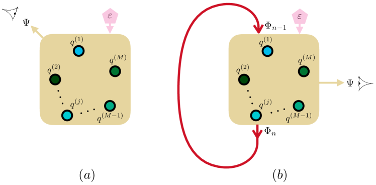
We consider high-dimensional systems composed of $M\gg 1$ chaotic microscopic degrees of freedom $q^{(j)}$, $j=1,\cdots,M$, which evolve in discrete time $n$ according to their individual parameters $a^{(j)}$. These degrees of freedom, evolving in isolation, may or may not obey LRT. We restrict our study of LRT to macroscopic observables

$$\Psi_{n}=\Psi(q^{(1)}_{n},q^{(2)}_{n},\cdots,q^{(M)}_{n}).$$ (1)

We consider in particular a mean field observable

$$\Psi_{n}=\frac{1}{M}\sum_{j=1}^{M}\psi(q^{(j)}_{n}),$$ (2)

where $\psi$ is some observable of the microscopic variable. We consider here smooth observables (at least Hölder continuous), which ensures that the statistical limit laws we later invoke exist. We consider here two scenarios, illustrated in Figure 1, where the perturbations of size $\varepsilon$ are globally applied to the dynamics: the case where the dynamics of the $q^{(j)}_{n}$ are uncoupled with

$$q^{(j)}_{n+1}=f(q^{(j)}_{n};a^{(j)},\varepsilon),$$ (3)

and the case where the dynamics of the $q^{(j)}_{n}$ are coupled by a mean field $\Phi$ with

$$q^{(j)}_{n+1}=f(q^{(j)}_{n},\Phi_{n};a^{(j)},\varepsilon),$$ (4)

where the coupling mean field is given by

$$\Phi_{n}=\frac{1}{M}\sum_{j=1}^{M}\phi(q^{(j)}_{n})$$ (5)

for some function $\phi$. Note that we explicitly distinguish between the macroscopic observable $\Psi_{n}$ and the dynamic variable $\Phi_{n}$. In our numerical simulations we did not find any difference in their respective LRT properties; the distinction, however, is instructive for the theoretical considerations provided later.

For each of the two scenarios we study the linear response of $\Psi$ for three different types of the microscopic dynamics $f$. We consider the case of microscopic dynamics which when viewed in isolation obeys LRT, such as uniformly expanding maps (the specific maps we will study are described in Section VI.2.1). We then consider the case when the microscopic dynamics when viewed in isolation does not obey LRT. The simplest such system is the logistic map as established by Baladi and co-workers Baladi and Smania (2008, 2010); Baladi (2014); Baladi, Benedicks, and Schnellmann (2015); De Lima and Smania (2018). We shall distinguish two subcases here; one where the parameters of the logistic map are drawn from a smooth heterogeneous distribution and one where they are drawn from a non-smooth distribution. For concreteness, we consider perturbations of the following modified logistic map,

$${\small{\left(q_{n+1}^{(j)},r_{n+1}^{(j)}\right)=\begin{cases}\left(q_{n}^{(j)},2r_{n}^{(j)}\right)&r_{n}^{(j)}<\tfrac{1}{2}\\ \left(a^{(j)}\,q_{n}^{(j)}(1-q_{n}^{(j)})+h(q^{(j)}_{n},\Phi_{n})+\varepsilon g(q^{(j)}_{n}),2r_{n}^{(j)}-1\right)&r_{n}^{(j)}\geq\tfrac{1}{2}\end{cases}}},$$ (6)

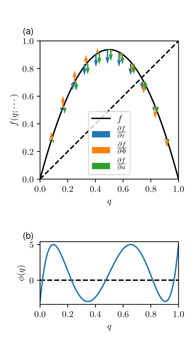
where the logistic map parameters $a^{(j)}$ are sampled from a distribution $\nu(a)da$ Wormell and Gottwald (2018). The action of this map on $q$ is plotted in Figure 3(a). To investigate the linear response properties of this system we choose the perturbation function

$$g(q^{(j)}_{n})=4(q^{(j)}_{n}(1-q^{(j)}_{n}))^{2}.$$ (7)

The function $h(q^{(j)}_{n},\Phi_{n})$ denotes the mean field coupling which is set to $h\equiv 0$ in the uncoupled scenario. In the coupled scenario we will consider the mean field coupling

$$h(q^{(j)}_{n},\Phi_{n})=(1-2q^{(j)}_{n})q^{(j)}_{n}(1-q^{(j)}_{n})\tanh\Phi_{n}.$$ (8)

The effect of $g$ and $h$ are also plotted in Figure 3(a).

We remark that a naive choice of mean field coupling with $h=\Phi_{n}$ would just lead back to the standard logistic map for some $p^{(j)}_{n}=\alpha q^{(j)}_{n}+\beta$ with a modified logistic map parameter $a^{(j)}=a^{(j)}(\Phi_{n})$. The mean field $\Phi_{n}$ is given by (5) and is constructed using

$$\phi(q)=4T_{5}(2q-1)+1,$$

where $T_{5}(x)=16x^{5}-20x^{3}+5x$ is the 5th Chebyshev polynomial, which oscillates between $\pm 1$ in the domain (see Figure 3(b)).

In our numerical simulations we use $\psi(q,r)=q$ for our mean-field observable $\Psi$.

The inclusion of the mixing doubling map dynamics $r_{n}$ ensures that the overall dynamics is mixing even when the logistic parameters $a^{(j)}$ correspond to regular dynamics. The inclusion of the cocycle $r_{n}$, however, does not alter the invariant measure of the logistic map for constant $\Phi_{n}$ and the marginal invariant measure of $q^{(j)}$ the invariant measure of a logistic map at parameter $a^{(j)}$. Hence, notwithstanding any dynamics of $\Phi_{n}$, the microscopic dynamics (6) violates LRT while being mixing.

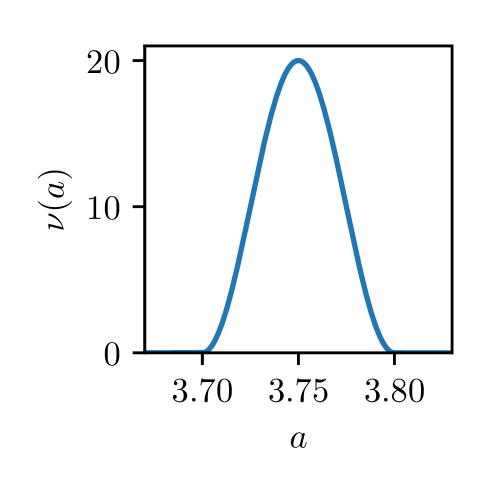
In Wormell and Gottwald (2018) it was established that the heterogeneity of the parameters $a^{(j)}$, as exemplified by the regularity of $\nu(a)$, was crucial in establishing LRT (albeit in a different, less general setting). We therefore consider here two cases: the case when $\nu(a)$ is smooth, in particular at least once-differentiable with respect to $a$, and the case when $\nu(a)$ is non-smooth, for example when $\nu(a)$ is a linear combination of delta functions. Similar to Wormell and Gottwald (2018) we choose as a smooth distribution the raised cosine distribution supported on the interval $[3.7,3.8]$, which is given by

$$\nu(a)=\mathbf{1}_{[3.7,3.8]}\frac{1}{0.1}\left(1+\cos\left(\frac{a-3.75}{0.05}\pi\right)\right).$$ (9)

We have chosen this distribution as it is both compactly supported and resembles a Gaussian distribution (see Figure 2). For a non-smooth distribution we choose the discrete distribution

$$\nu=\frac{1}{3}(\delta_{3.72}+\delta_{3.75}+\delta_{3.78}),$$ (10)

which has a similar distribution of moments.

Figure 2: Probability density function $\nu(a)$ of the raised cosine distribution (9) with compact support on the interval $[3.7,3.8]$.

Figure 3: (a) Plot of $q^{(j)}_{n+1}$ under logistic dynamics (6) as a function of $q^{(j)}_{n}$ for $r^{(j)}_{n}>1/2,\,a^{(j)}=3.75,\,\Phi_{n}=0$ and $\varepsilon=0$. Effects of perturbations in $\varepsilon$, $\Phi$ and $a$ on the map are indicated by arrows. (b) Plot of coupling function $\phi(q)$.

IV Summary of results

Our main results for these different dynamical scenarios and cases are summarised in Table 1. We differentiate between the thermodynamic limit $M=\infty$ and the case of a large, finite heat bath size $M$ (which may not necessarily approach a smooth limit as $M\to\infty$). We summarise the dynamical mechanisms leading to the comprehensive picture provided in Table 1, which are to the best of our knowledge hitherto unknown. The following sections will establish these findings in detail.

• Macroscopic mean field observables generated by an appropriate heterogeneous set of microscopic chaotic systems may exhibit linear response, even if the individual members of those systems may not individually have LRT (Section V.2.2).

• In the thermodynamic limit, macroscopic observables obey a law of large numbers. If the microscopic dynamics is mixing, this leads in the case of no back-coupling to trivial macroscopic dynamics (Section V.1); if the microscopic dynamics is coupled via its mean field and provided the microscopic dynamics collectively obeys LRT, one can derive a smooth non-Markovian closure for macroscopic variables (Section VI.1). In the latter case, if the macroscopic dynamics converges to a fixed point or to a limit cycle, the macroscopic mean field observables satisfy LRT in the thermodynamic limit (Section VI.2). However, the reduced macroscopic dynamics may also converge to a chaotic dynamical system which violates LRT. This is possible even if the individual microscopic dynamics is uniformly hyperbolic (Section VI.3).

• In finite ensembles with $M<\infty$ the mean field involves an ${\mathcal{O}}(1/\sqrt{M})$ correction to the thermodynamic mean field dynamics, which may not obey LRT (Section V.1). The possible violation of LRT of macroscopic observables, however, is not detectable for practical purposes, and the observed linear response is determined by the linear response property of the thermodynamic limit. We call this behaviour approximate LRT.

• In finite mean-field coupled systems such as (4), macroscopic mean fields typically satisfy a central limit theorem. As a result, the back-coupling of the mean field introduces a small “noise” into the microscopic systems, which can induce linear response. The statistical properties of this dynamic self-generated noise and its linear response properties are determined by the linear response property of the thermodynamic limit. In the case of failure of linear response in the thermodynamic limit, the convergence to the thermodynamic limit is approached for finite large $M$ through the creation of saddle-node bifurcations (with associated multistability) which become increasingly dense in $\varepsilon$ (Section VI.2.3).

		macroscopic observables
microscopic subsystem		uncoupled	coupled
$f$ satisfies LRT	finite $M$	✓	✓
	$M\to\infty$	✓	✯
$f$ violates LRT with smooth $\nu(a)da$	finite $M$	(✓)	(✓)
	$M\to\infty$	✓	✯
$f$ violates LRT with non-smooth $\nu(a)da$	finite $M$	✗	(✓)
	$M\to\infty$	✗	✗

Table 1: Summary of our main result. The checkmarks ✓  denote cases when the macroscopic observable $\Psi$ enjoys LRT. The bracketed checkmarks (✓)  denote cases of approximate LRT, when LRT is satisfied for practical purposes. The cross-marks ✗  denote cases when LRT is violated for the macroscopic observable. The star ✯  denotes cases when LRT may or may not be satisfied depending on the linear response of the limiting dynamics of the macroscopic observable (see Section VI).

In the following we provide numerical evidence and theoretical arguments corroborating these results. We first consider the case of macroscopic observables of an uncoupled heat bath before considering the case of macroscopic observables of a mean field coupled heat bath.

V Macroscopic observables of uncoupled microscopic subsystems

We are concerned with the behaviour of averages of the macroscopic observable $\Psi$. We distinguish here two averages; the average with respect to initial conditions of $q^{(j)}$, which we denote by $\mathbb{E}$, and the average over the independently chosen logistic map parameters distributed according to $\nu(a)$ which we denote by angular brackets $\langle\cdot\rangle$. In real systems (for which the parameters $a^{(j)}$ are selected once only), the average relevant for linear response is $\mathbb{E}$, the expectation with respect to initial conditions.

We describe a stochastic reduction of the mean field dynamics in Section V.1 and then in Section V.2 discuss the linear response properties for each of the three kinds of microscopic subsystems that we outlined in Section III: in Table 1 these are covered in the rows corresponding to the uncoupled macroscopic observables.

V.1 Stochastic reduction of mean field dynamics

The average with respect to initial conditions is written as

$$\mathbb{E}\psi(q^{(j)})=\int\psi(q)d\mu^{a^{(j)}}(q),$$

where $\mu^{a^{(j)}}(q^{(j)})$ is the invariant measure of $q^{(j)}$. The Law of Large Numbers then reads as

$$\langle\mathbb{E}\Psi\rangle=\iint\psi(q)d\mu^{a}(q)d\nu(a).$$ (11)

(In view of Section VI where the mean field coupling is considered and the $q^{(j)}$ depend on a time-varying driver, we remark that in that case averages are computed with a time dependent measure $\mu^{a^{(j)}}_{n}(q^{(j)})$.)

We first establish the case of LRT for a finite heat bath. For large but finite system size $M$, both averages are equipped with their own finite size correction, described by the central limit theorem. In equilibrium each ensemble member $q^{(j)}_{n}$, at a given time $n$, is an independent sample from the invariant measure $\mu^{a^{(j)}}$. Macroscopic observables $\Psi$, as defined in (2), can be approximated using the central limit theorem and the independence of the $q^{(j)}$ by

$$\Psi_{n}=\mathbb{E}\Psi+\frac{1}{\sqrt{M}}\zeta_{n}+o(1/\sqrt{M}),$$ (12)

where the expectation value

$$\mathbb{E}\Psi=\frac{1}{M}\sum_{j=1}^{M}\int\psi(q)d\mu^{a^{(j)}}(q)$$

is over initial conditions $q^{(j)}$ at fixed $a^{(j)}$. The random mean-zero Gaussian process $\zeta_{n}$ has autocovariance function $C^{\zeta}(m)$ with

$$C^{\zeta}(m) =\operatorname{cov}(\zeta_{n},\zeta_{n+m})=\lim_{M\to\infty}\frac{1}{M}\sum_{j=1}^{M}\mathbb{E}[\psi^{(j)}_{0}\psi^{(j)}_{m}]$$

$$=\langle\mathbb{E}[\psi_{0}\psi_{m}]\rangle.$$ (13)

The existence of a central limit theorem is guaranteed for unimodal maps using results of Lyubich Lyubich (2002) who proved that almost every non-regular logistic parameter satisfies the so-called Collet-Eckmann condition Collet and Eckmann (1983), which then implies the existence of good statistical properties including the central limit theoremAlves, Luzzatto, and Pinheiro (2004); Melbourne and Nicol (2008). We remark that the parameters determining the process $\zeta_{n}$ in the finite-$M$ case, such as the covariance (13), have the same LRT properties as the associated thermodynamic limit $\langle\mathbb{E}^{\varepsilon}\Psi\rangle$.

The independent sampling of the $a^{(j)}$ allows for a further application of the central limit theorem, and we can write

$$\mathbb{E}\Psi_{n}=\langle\mathbb{E}\Psi_{n}\rangle+\frac{1}{\sqrt{M}}\eta+o(1/\sqrt{M}),$$ (14)

where the random variable $\eta$ is, for fixed $\varepsilon$, a mean-zero Gaussian variable. As a function of $\varepsilon$, $\eta$ is a Gaussian process with covariance

$$\langle\eta^{\varepsilon}\eta^{\varepsilon^{\prime}}\rangle=\langle\mathbb{E}^{\varepsilon}[\psi]\mathbb{E}^{\varepsilon^{\prime}}[\psi]\rangle-\langle\mathbb{E}^{\varepsilon}[\psi]\rangle\langle\mathbb{E}^{\varepsilon^{\prime}}[\psi]\rangle,$$ (15)

and typically is no more differentiable with respect to $\varepsilon$ than $\mathbb{E}^{\varepsilon}[\psi]$, which implies that LRT is violated for finite $M$ if the microscopic subsystems do not individually satisfy LRT. However, for finite $M\gg 1$ the response term $\langle\mathbb{E}\Psi_{n}\rangle$ dominates over the contribution of $\eta$ and the violation of LRT can only be detected for vanishingly small values of $\varepsilon$. We call this instance of LRT for all practical purposes approximate LRT.

We remark that, notwithstanding the rough parameter selection error discussed above, and recalling that the linear response of the process $\zeta_{n}$ is determined by the linear response property of the associated thermodynamic limit, the overall linear response of $\Psi_{n}$ depends entirely on whether the thermodynamic limit $\langle\mathbb{E}\Psi_{n}\rangle$ satisfies LRT or not. We discuss this question in the next section.

V.2 LRT of thermodynamic limit mean field observables of uncoupled microscopic subsystems

We now investigate the response of $\langle\mathbb{E}\Psi_{n}\rangle$, i.e. the thermodynamic limit. We distinguish between three cases: when the microscopic dynamics satisfies LRT, and when the the microscopic dynamics does not satisfy LRT and has a distribution $\nu(a)$ of the parameters which is either smooth or non-smooth.

V.2.1 The microscopic subsystems satisfy LRT

If the microscopic dynamics obeys LRT, as is the case for uniformly expanding maps such as (32), which will be considered in Section VI.2.1, it is clear that LRT also holds for macroscopic observables defined in (2). For finite heat bath sizes $M$, we have

$$\frac{d}{d\varepsilon}\mathbb{E}^{\varepsilon}\Psi_{n}=\frac{1}{M}\sum_{j=1}^{M}\frac{d}{d\varepsilon}\mathbb{E}\psi(q^{(j)}_{n})$$

and the macroscopic observable $\Psi$ has LRT since the $M$ subsystems individually satisfy LRT with uniformly bounded $\frac{d}{d\varepsilon}d\mu^{(a_{j},\varepsilon)}$. The validity of LRT carries over to the thermodynamic limit with

$$\frac{d}{d\varepsilon}\langle\mathbb{E}^{\varepsilon}\Psi_{n}\rangle =\iint\psi^{\varepsilon}(q)\frac{d}{d\varepsilon}d\mu^{(a,\varepsilon)}(q)\nu(a)da.$$

Note that we may allow for a $\nu$-measure zero subset of subsystems at any given $\varepsilon$ to individually violate LRT, and still obtain LRT for the macroscopic observable $\Psi$ in the $M\to\infty$ limit. In this case, however, the $\eta$ correction may not be differentiable, and we observe approximate LRT.

V.2.2 The microscopic subsystems do not satisfy LRT but are appropriately heterogeneous

As typical microscopic dynamics leading to violation of LRT we consider the modified logistic map (6), which is perturbed in $\varepsilon$ by the function (7), and whose parameters are drawn from the smooth raised cosine distribution (9) which is three-times continuously differentiable (i.e. $\nu(a)$ is $C^{3}$).

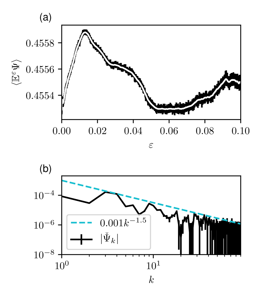
Figure 4 provides numerical evidence that, for these maps, the macroscopic observable $\Psi$ with $\psi(x)=x$ has linear response for a wide range in $\varepsilon$. To determine the smoothness of $\langle\mathbb{E}^{\varepsilon}\Psi\rangle$, we determine its Chebyshev coefficients on a Chebyshev roots grid of $1000$ points. It is well known that any smooth function $f(x)$ can be expressed as an infinite series of Chebyshev polynomials $T_{k}(x)$ as $f(x)=\sum_{k=0}^{\infty}f_{k}T_{k}(x)$ and the degree of differentiability of the function is given by the decay of its Chebyshev coefficients $f_{k}$ Trefethen (2013). We find that the Chebyshev coefficients of $\langle\mathbb{E}^{\varepsilon}\Psi\rangle$ decay as $\mathcal{O}(k^{-4})$, which is indicative of $\langle\mathbb{E}^{\varepsilon}\Psi\rangle$ being between $C^{3^{-}}$ and $C^{4}$ differentiable over a large interval: this level of differentiability, as we will see below, is connected to the smoothness of the raised-cosine distribution (9), which is $C^{3}$ Wormell and Gottwald (2018). We have also employed the test statistics for higher-order linear response developed in Gottwald, Wormell, and Wouters (2016) to test the null-hypothesis of $\langle\mathbb{E}^{\varepsilon}\Psi\rangle$ being well-approximated by a linear combination of $T_{k}(0.1^{-1}(\varepsilon+0.1)),k=0,\ldots,60$ for $\varepsilon\in[-0.2,0]$, i.e. that the response is in fact a smooth function. This test is summarised in Appendix A. We used the aforementioned Chebyshev grid simulating $1,000,000$ different randomly selected parameters with $50$ runs of $3000$ timesteps each, and quantified Birkhoff variance both within parameters and between parameters (i.e. arising from the random parameter selection), using standard ANOVA methods Rice (2006). We obtain a $p$-value of $0.26$, consistent with the null-hypothesis of a smooth response.

Figure 4: Response term $\mathbb{E}^{\varepsilon}\Psi$ for a perturbation of the form (7) for an uncoupled heat bath scenario in the case when the microscopic dynamics is given by the logistic map (6), which does not satisfy LRT, and the logistic map parameters are sampled from the raised cosine distribution (9). For different values of $\varepsilon$ we employ a total of $10^{5}$ iterates to estimate $\mathbb{E}^{\varepsilon}\Psi$ as a temporal average. (a) Plots for finite $M$: 95% confidence intervals were estimated from $10$ realisations differing in the initial conditions of the heat bath, and are not visible. Thermodynamic limit curve (black), confidence intervals also not visible, was estimated from $50$ realisations of $3000$ iterates for $10^{6}$ parameters $a^{(j)}$ independently selected for each $\varepsilon$. (b) Thermodynamic limit of $\mathbb{E}^{\varepsilon}\Psi$ (black), with LRT-violating response of microscopic variables $\mathbb{E}^{\varepsilon}\psi(q^{(j)})$ (coloured lines), estimated from $10$ realisations of $10^{6}$ iterates each. (c) Estimate of Chebyshev coefficients $\sum_{k=0}^{\infty}\check{\Psi}_{k}T_{k}(0.1^{-1}(x+0.1)):=\langle\mathbb{E}^{\varepsilon}\Psi\rangle$.

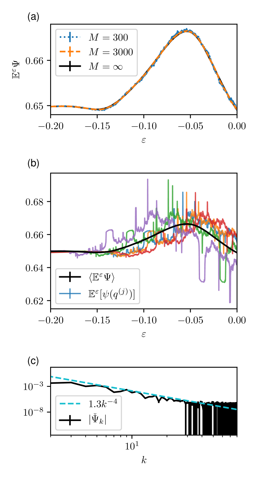
We note that in Figure 4 the response of $\mathbb{E}^{\varepsilon}\Psi$ for systems with finite $M$ have (barely) noticeable rough deviations from the $M\to\infty$ limit: these non-smooth deviations arise from the finite sampling of parameters $a^{(j)}$ from $\nu(a)$, approximated by the random variable $\eta$ defined in (14), as discussed above.

We now provide a heuristic argument how averaging over a smooth distribution such as the raised cosine distribution (9) can lead to LRT for the macroscopic observable $\Psi$. Let us first recall the dynamic reason of why LRT is violated in the logistic map. We follow here Ruelle (2009b) in our exposition. The critical point $q=c$ with $f^{\prime}(c)=0$ leads to a non-uniform compression of the phase space around $q=c$: an initially smooth initial density which contains the critical point in its support is pushed forward under the dynamics to a non-smooth density with a spike with an inverse square-root singularity at $q=f(c)$. This compression is repeated to produce further inverse square-root singularities at locations $q_{n}=f^{n}(c)$ of amplitudes asymptotically proportional to $\alpha^{-n/2}$ (and thus contain a probability mass of order $\alpha^{n/2}$), where $1<\alpha$ denotes the Lyapunov multiplier of the logistic map. The result is that the invariant density contains an infinite number of spikes of decreasing amplitude. The effect of the perturbation, by modifying the forward orbit of the critical point $(f^{n}(c))_{n\in\mathbb{N}}$, is to displace these spikes. Because the map $f$ is chaotic and thus exponentially sensitive to perturbations, spikes move with an instantaneous speed of the order of $\alpha^{n}$ per unit change of the perturbation. This scenario is illustrated in Figure 5(a) where we show the absolutely continuous invariant measure (acim), averaged over the heat bath, of an perturbed and of a slightly perturbed dynamics. The high speed of the small spikes (i.e. those with large $n$) in conjunction with their relatively large probability mass implies that the sum of their (distributional) derivatives diverges, leading to breakdown of linear response. The reader is referred to Ruelle (2009b) for details and to Gottwald, Wormell, and Wouters (2016) for a numerical illustration. For comparison we also depict in Figure 5(b) the averaged invariant measure for the case when the parameters are heterogeneously drawn from a raised-cosine distribution and for which we showed above that LRT is valid. The averaging over the heterogenously drawn parameters clearly implies a smoothed invariant measure of the logistic map.

This may be seen as analogous to a recent heuristic argument for linear response in general non-hyperbolic systemsRuelle (2018): rough contributions to the response caused by singularities in the physical measures that arise from stable manifold-unstable manifold tangencies average out if these singularities distribute themselves suitably evenly.

In the specific case where the microscopic dynamics evolves under unimodal maps such as those studied here, we can make a more concrete argument for the effect of the smearing out of the fast displacement of the small spikes upon perturbation. It is conjectured by Avila et al Avila, Lyubich, and de Melo (2003), there exists an $\varepsilon$-dependent analytic function $\alpha(a,\varepsilon)$ of the invariant measures, such that the map with parameters $(a,\varepsilon)$ is topologically conjugate to the map with parameters $(\alpha(a,\varepsilon),0)$. Unimodal maps, at least those of Benedicks-Carleson type, have linear response within topological conjugacy classes Baladi and Smania (2012), and as a result we can say

$$\langle\mathbb{E}^{\varepsilon}\Psi\rangle =\iint\psi(q)d\mu_{n}^{a,\varepsilon}\nu(a)da$$

$$=\iint\psi(q)d\mu_{n}^{\alpha(a,\varepsilon),0}\nu(a)da+\mathrm{h.o.t.}$$

$$=\iint\psi(q)d\mu_{n}^{\alpha,0}\nu(a(\alpha,\varepsilon))\frac{da}{d\alpha}d\alpha+\mathrm{h.o.t.},$$ (16)

where the higher order terms capture the response of the $\mu_{n}$ under the topological conjugacy-preserving parameter change from $(\alpha(a,\varepsilon),0)$ to $(a,\varepsilon)$, and are thus similarly smooth. Hence the existence of linear response $d\langle\mathbb{E}^{\varepsilon}\Psi\rangle/d\varepsilon$ (and by a similar argument higher-order response) is guaranteed, provided that the distribution of the parameters of the logistic map $\nu(a)$ is at least once continuously differentiable (and provided $\alpha(a,\varepsilon)$ is analytic in a sufficiently uniform wayAvila, Lyubich, and de Melo (2003)). The linear response of $\langle\mathbb{E}^{\varepsilon}\Psi\rangle$ was numerically confirmed in Figure 4. Since in at least one-dimensional systems topological conjugacy classes form manifolds of finite codimension, we believe this argument will generalise to more general maps, provided the space of parameters $a^{(j)}$ is sufficiently high-dimensional.

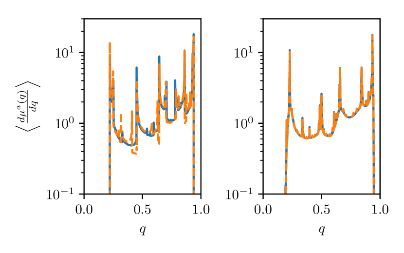
(a)                                                  (b)

Figure 5: Histogram of the averaged acim of the $q^{(j)}$ for the logistic map system (6) with (a) $\nu=\delta_{3.75}$ and (b) $\nu$ the raised-cosine distribution (9), for $\varepsilon=-5\times 10^{-4}$ (orange dashes) and $\varepsilon=0$ (blue line).

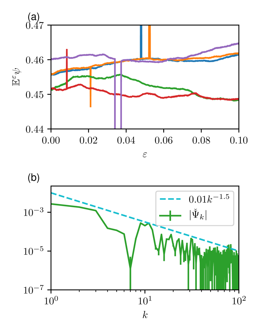
However, we caution that our smearing argument may not generalise to other systems, at least when the support of the parameters $a$ is one-dimensional. In Figure 6 we present numerical evidence demonstrating that mean-field averaging fails to improve the linear response of a unimodal map of the torus $({\mathbb{R}}/{\mathbb{Z}})^{2}$ for heterogeneously distributed parameters, given by

$$x^{(j)}_{n+1} =x^{(j)}_{n}+a^{(j)}y\sin\pi x^{(j)}_{n}\mod 1$$ (17)

$$y^{(j)}_{n+1} =y^{(j)}_{n}+a^{(j)}\sin\pi(x^{(j)}_{n}+y^{(j)}_{n})+\varepsilon\mod 1,$$ (18)

for $j=1,\ldots,M$. The parameters $a^{(j)}$ are again distributed according to a raised cosine distribution with support on $[3.7,4.3]$

$$\nu(a)=\mathbf{1}_{[3.7,4.3]}\frac{1}{0.1}\left(1+\cos\left(\frac{a-3}{0.3}\pi\right)\right),$$ (19)

and the mean-field observable is given by $\Psi=\frac{1}{M}\sum_{j=1}^{M}\psi(x^{(j)},y^{(j)})$ where $\psi(x,y)=x$, as before. We tested the null-hypothesis of $\langle\mathbb{E}^{\varepsilon}\Psi\rangle$ being well-approximated by a linear combination of $T_{k}(0.05^{-1}(\varepsilon-0.05)),k=0,\ldots,100$ for $\varepsilon\in[0,0.1]$, and obtained a p-value $p=0.49$, consistent with the null hypothesis. However in Figure 6 we see that the estimated Chebyshev coefficients decay approximately as $\mathcal{O}(k^{-1.5})$ which is slower than $\mathcal{O}(k^{-4})$ seen in the one-dimensional unimodal example, indicating a rather low-order differentiability. This level corresponds quite closely to that obtained for the expectation value $\mathbb{E}^{\varepsilon}\psi(x^{(j)},y^{(j)})$ of a single microscopic systems, as illustrated in Figure 7; hence the averaging over parameters appears only to be smoothing out the large jumps arising from periodic windows but does not improve the degree of differentiability.

Figure 6: Response term $\mathbb{E}^{\varepsilon}\Psi$ for an uncoupled heat bath scenario for the map (18) where the parameters are sampled from a raised cosine distribution (19). (a) Infinite $M$ limit with confidence intervals (black) and $21$-point moving average with confidence intervals (white) from $15$ realisations of $6000$ iterates for $10^{6}$ parameters $a^{(j)}$ independently selected for each $\varepsilon$. (b) Estimate of Chebyshev coefficients $\sum_{k=0}^{\infty}\check{\Psi}_{k}T_{k}(0.05^{-1}(x+-0.05)):=\langle\mathbb{E}^{\varepsilon}\Psi\rangle$.

Figure 7: Individual response terms $\mathbb{E}^{\varepsilon}\psi(x^{(j)},y^{(j)})$ with confidence intervals for the map (18) where the parameters selected from the raised cosine distribution (19). (a) Response for five randomly selected microscopic variables. The large jumps of the response outside the figure correspond to regions of regular dynamics. (b) Estimate of Chebyshev coefficients $\sum_{k=0}^{\infty}\check{\Psi}_{k}T_{k}(0.05^{-1}(x+-0.05)):=\langle\mathbb{E}^{\varepsilon}\Psi\rangle$ for one of the variables in (a).

V.2.3 The microscopic subsystems do not satisfy LRT and are not appropriately heterogeneous

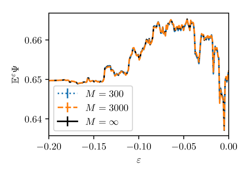
If the microscopic dynamics does not obey LRT and the logistic map parameters are non-smoothly distributed, then LRT fails for macroscopic observables (2), independent of whether the heat bath is finite or infinite. In this case the averaging over the heat bath variables does not provide the necessary smearing of the non-smoothness of the perturbed invariant measures $\mu^{a,\varepsilon}$. To illustrate this, consider the following non-smooth parameter distribution

$$\nu(a)=\sum_{k=1}^{p}w_{k}\delta(a-a_{k}),$$ (20)

where at least one of the logistic map parameters $a_{k}$ corresponds to chaotic dynamics. The invariant measures $\mu^{a_{k},\varepsilon}$ for fixed parameters $a_{k}$ are not differentiable with respect to the perturbation size $\varepsilon$ per assumption. The averaging over the independent heat bath variables only involves finitely many logistic parameter values, and hence in this situation averaging is not able to smear the effect of the non-smoothness of the finite number of associated invariant measures $\mu^{a_{j}}$. In Figure 8 we show the response $\mathbb{E}^{\varepsilon}\Psi$ which as expected exhibits non-smooth behaviour upon varying the strength of the perturbation $\varepsilon$. The response term $\mathbb{E}^{\varepsilon}\Psi$ quickly converges and for $M=300$ is almost indistinguishable by eye from the response $\langle\mathbb{E}^{\varepsilon}\Psi\rangle$ in the thermodynamic limit.

Figure 8: Response term $\mathbb{E}^{\varepsilon}\Psi$ for a perturbation of the form (7) for an uncoupled heat bath scenario in the case when the microscopic dynamics is given by the logistic map (6), which does not satisfy LRT, and the logistic map parameters are distributed as in (20) with $\nu=\tfrac{1}{3}(\delta_{3.72}+\delta_{3.75}+\delta_{3.78})$. Error bars were estimated from $10$ realisations differing in the initial conditions of the heat bath, and are not visible.

VI Linear response of macroscopic observables of microscopic subsystems with mean field coupling

We now consider the case when the heat bath variables $q^{(j)}$ couple via the mean field $\Phi_{n}$. In Section VI.1 we derive a non-Markovian closure of the mean-field dynamics, along the lines of the reduction derived in Section V, that is deterministic in the thermodynamic limit and stochastic for finite $M$; in Sections VI.2 and VI.3 we study the mean-field dynamics and its linear response using this macroscopic closure.

VI.1 Surrogate approximation of the mean field dynamics

Before we can study the response of the mean field coupled system to external perturbations $\varepsilon g$, we need to understand the implied macroscopic dynamics $\Phi_{n}$ generated by the system for the externally unperturbed system with $\varepsilon=0$. To do so we view the system as driven by a prescribed time-dependent external driver $d_{n}$ rather than the mean field $\Phi_{n}$, as illustrated in Figure 9 (which should be compared with Figure 1(b)). Hence we replace the mean field coupled dynamics (4) by

$$q^{(j)}_{n+1}=f(q^{(j)}_{n},d_{n};a^{(j)},\varepsilon)$$ (21)

for a prescribed external driver $d_{n}$. In the thermodynamic limit of the mean field coupled system (4) we will see that the macroscopic mean field dynamics is deterministic (see (29) further down), and the driver $d_{n}=\Phi_{n}$ is indeed prescribed by the initial conditions, which is simply the initial distribution of the $q^{(j)}$. For large but finite $M$, the $q^{(j)}_{n}$ conditioned on the history of the mean field $(\Phi_{n-1},\ldots)$ can be considered as independently distributed and one can again view the mean field $\Phi_{n}$ as an externally prescribed noisy driver $d_{n}$ with specified statistical properties. The surrogate system (21) with the external driver $d_{n}$ chosen as a random draw of the Gaussian process (defined below in (22)) provides an accurate representation of the statistical behaviour of the original mean field coupled system (4). We have checked that both yield the same linear response $\mathbb{E}^{\varepsilon}\Psi$, and now set out to study the linear response of the original mean field coupled system via the surrogate system.

Let us now determine the statistical properties of a macroscopic mean field observable for the driven surrogate system (21). The mean fields $\Phi_{n}$ and $\Psi_{n}$ are again Gaussian process with (now time-dependent) statistical properties given again by statistical limit laws, and we write in particular

$$\Phi_{n}=\langle\mathbb{E}^{d}[\Phi_{n}]\rangle+\frac{1}{\sqrt{M}}\zeta_{n}+\frac{1}{\sqrt{M}}\eta_{n}+o\left(\frac{1}{\sqrt{M}}\right),$$ (22)

where

$$\mathbb{E}^{d}[\Phi_{n}]=\mathbb{E}[\Phi_{n}|d_{k};\,k<n]$$ (23)

denotes the conditional expectation over the past history of the driver and averages now involve time-dependent measures $\mu_{n}^{a^{(j)}}$. The autocovariances of the mean-zero Gaussian process $\zeta_{n}$ are given by a central limit theorem approximation of $\Phi_{n}-\mathbb{E}^{d}[\Phi_{n}]$ with

$$\operatorname{cov}[\zeta_{n},\zeta_{n-k}]=\langle\operatorname{cov}[\phi(q^{(j)}_{n}),\phi(q^{(j)}_{n-k})]\rangle,$$ (24)

where the covariance is defined using the conditional average over the history of the driver (cf. (13)). Note that the autocovariance is not a function of $n-m$ due to the non-Markovian nature of the dynamics. Similarly, a central limit theorem approximation of $\mathbb{E}^{d}[\Phi_{n}]-\langle\mathbb{E}^{d}[\Phi_{n}]\rangle$, defines the mean-zero Gaussian process $\eta_{n}$ with autocovariance

$$\langle\eta_{n}^{\varepsilon},\eta_{m}^{\varepsilon^{\prime}}\rangle=\langle\mathbb{E}^{d,\varepsilon}[\phi(q^{(j)}_{n})]\mathbb{E}^{d,\varepsilon^{\prime}}[\phi(q^{(j)}_{m})]\rangle-\langle\mathbb{E}^{d,\varepsilon}[\phi(q^{(j)}_{n})]\rangle\langle\mathbb{E}^{d,\varepsilon^{\prime}}[\phi(q^{(j)}_{m})]\rangle,$$ (25)

where again the conditional expectation values $\mathbb{E}$ are used (cf. (15)). Note that the Gaussian processes $\zeta_{n}$ and $\eta_{n}$ are independent.

The impulsive response of $\Phi_{n}$ at a given time to a perturbation of the driving process $d_{n}\mapsto d_{n}+\theta_{n}$, where $|\theta_{n}|\ll 1$, can be, at least formally, captured by the susceptibility function

$$R_{n}(z)=\sum_{k=1}^{\infty}\chi_{n,k}\,z^{k},$$ (26)

defined for complex $z$ with $|z|\leq 1$ Ruelle (2004). The fluctuation coefficients $\chi_{n,k}$ describe the change of the mean field induced by the drivers $\theta_{n}$ as

$$\langle\mathbb{E}^{d+\theta}[\Phi_{n}]\rangle-\langle\mathbb{E}^{d}[\Phi_{n}]\rangle=\sum_{k=1}^{\infty}\chi_{n,k}\,\theta_{n-k}.$$ (27)

The fluctuation coefficients $\chi_{n,k}$ of $\Phi_{n}$ are given as an average over the microscopic fluctuation coefficients $\chi_{n,k}^{a}$ of $\phi(q^{(j)}_{n})$ as

$$\chi_{n,k}=\int\chi_{n,k}^{a}\,\nu(a)da.$$ (28)

A necessary condition for LRT with respect to a bounded driver $\theta_{n}$ is the summability of the coefficients $\chi_{k}$. Once LRT with respect to the driver $d_{n}$ can be shown, we can proceed to study the linear response with respect to the external perturbation with $\varepsilon\neq 0$ (recall that $d_{n}=\Phi_{n}$ (cf. Figure 1)). Note that if $\langle\mathbb{E}^{d}[\Phi_{n}]\rangle$ does not satisfy LRT with respect to a perturbation of the driver $d_{n}$, then it cannot be expected to satisfy LRT with respect to external perturbation.

Figure 9: Sketch of the macroscopic dynamics $\Phi_{n}$ mediated by the microscopic reservoir.

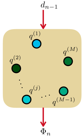
In the thermodynamic limit, provided the microscopic dynamics is mixing, we can use that the measures $\mu^{a}_{n}$ are the physical invariant measures generated by the cocycle $f(\cdot,\Phi_{n};a,\varepsilon)$ Froyland, Lloyd, and Quas (2013); Buzzi (1999) to create a closure of the dynamics of $\Phi_{n}$ as a deterministic recurrence relation:

$$\Phi_{n}=\langle\mathbb{E}^{d=\Phi}[\Phi_{n}]\rangle=:F(\Phi_{n-1},\Phi_{n-2},\ldots;\varepsilon).$$ (29)

If the mixing times of the $q^{(j)}$ are much shorter than a delay $k_{*}$, then the effect of the driving $\Phi_{n-k}$ for $k>k_{*}$ is minimal and the mean field dynamics is effectively Markovian in a space of dimension $k_{*}$ or less. The linear response with respect to perturbations, $\mathbb{E}^{\varepsilon}\Phi_{n}$, is now determined by the properties of the deterministic macroscopic dynamics (29). In the following sections we shall consider cases and conditions on the deterministic macroscopic dynamics (29) when $\mathbb{E}^{\varepsilon}\Phi_{n}$ enjoys linear response and when it does not.

For finite size $M$ the response approximates that of the thermodynamic limit, as in the case of an uncoupled heat bath discussed in Section V. However, The CLT approximation (22) assures that the microscopic dynamics (21), which is driven by $d_{n}=\Phi_{n}$, is essentially stochastic with a noise process $\zeta_{n}$ that has decay of temporal correlations (since the $q^{(j)}$ exhibit decay of correlations). This self-generated dynamic noise induces linear response for finite size mean field coupled heat baths, which can be seen as a consequence of results by Hairer and Majda Hairer and Majda (2010).

In Section VI.2-VI.3 we will consider the dynamics of the system in the thermodynamic limit. The first case is when $\Phi_{n}=\langle\mathbb{E}\Phi_{n}\rangle$ approaches a fixed point $\bar{\Phi}$ for $M\to\infty$, the second case is when the mean field $\Phi_{n}$ itself exhibits nontrivial dynamics. Whereas in the first case the linear response of the macroscopic observable $\Psi$ is determined by the properties of the microscopic dynamics, in the latter case it is entirely determined by the response of the macroscopic dynamics.

VI.2 Trivial dynamics of the mean field observable

Let us first look at the case of the mean field at a stable fixed point $\bar{\Phi}$, in the sense that the mean field remains bounded when perturbed from $\bar{\Phi}$ and, when the collective dynamics has LRT, $\bar{\Phi}$ is a stable fixed point of $\Phi_{n}$ in the thermodynamic limit.

To understand the stability, we can apply the external driving framework expounded in the previous section to the dynamics of our system about the equilibrium $d_{n}\equiv\bar{\Phi}$. Stability is in fact assured provided that the complex susceptibility function $R(z)$ does not have any roots inside the unit disk. This follows by considering $\theta_{n}=\langle\mathbb{E}\Phi_{n}\rangle-\bar{\Phi}=\sum_{k=0}^{\infty}\chi_{n,k}\theta_{n-k}$ with $\theta_{n}\sim\lambda^{n}$ in (27) which leads to

$$R(\lambda^{-1})-1=0,$$

and hence, for unstable $|\lambda|>1$, to the above condition for instability for the susceptibility function $R(z)$.

If stability is ensured, the linear response of the fixed point $\bar{\Phi}$ with respect to external perturbations $\varepsilon g$ is established by the implicit function theorem from the deterministic macroscopic dynamics (29). Once an external perturbation $\varepsilon g$ is applied, the fixed point depends on $\varepsilon$, and we write

$$0=F(\bar{\Phi}^{\varepsilon},\bar{\Phi}^{\varepsilon},\bar{\Phi}^{\varepsilon},\cdots;\varepsilon)-\bar{\Phi}^{\varepsilon}.$$ (30)

In the following numerical experiments the $M\to\infty$ limit is computed by estimating a solution to this algebraic equation.

Differentiation with respect to the external perturbation yields

$$0 =\frac{d\bar{\Phi}^{\varepsilon}}{d\varepsilon}\left(\frac{\partial}{\partial\bar{\Phi}^{\varepsilon}}F(\bar{\Phi}^{\varepsilon},\bar{\Phi}^{\varepsilon},\bar{\Phi}^{\varepsilon},\cdots;\varepsilon)-1\right)$$

$$\hphantom{=\;}+\frac{\partial}{\partial\varepsilon}F(\bar{\Phi}^{\varepsilon},\bar{\Phi}^{\varepsilon},\bar{\Phi}^{\varepsilon},\cdots;\varepsilon)$$

$$=\frac{d\bar{\Phi}^{\varepsilon}}{d\varepsilon}\left(\sum_{k=1}^{\infty}\chi_{k}-1\right)+\frac{\partial}{\partial\varepsilon}F(\bar{\Phi}^{\varepsilon},\bar{\Phi}^{\varepsilon},\bar{\Phi}^{\varepsilon},\cdots;\varepsilon).$$

This immediately yields that

$$\frac{d\bar{\Phi}^{\varepsilon}}{d\varepsilon}=\frac{\frac{\partial}{\partial\varepsilon}F}{1-R(1)},$$ (31)

and hence the existence of linear response, provided $R(1)-1\neq 0$.

As for the uncoupled scenario, we shall now discuss the linear response behaviour for the three different cases of the microscopic dynamics, which are covered by the rows in Table 1 corresponding to the coupled macroscopic observables.

VI.2.1 The microscopic subsystems satisfy LRT

We consider here the case of uniformly expanding dynamics of the microscopic systems, such that each subsystem individually satisfies LRT. In particular, we choose the following uniformly expanding map

$$q_{n+1}=\frac{T(q_{n})+K_{n}\left(1-\sqrt{0.03(1-0.97K_{n}^{2})+0.97(T(q_{n})+K_{n})^{2}}\right)}{1-0.97K_{n}^{2}},$$ (32)

where $K_{n}=\tanh(\varepsilon\Phi_{n}-2)$, $q_{n}\in[-1,1]$ and $T(q)=2q-\operatorname{sign}q$ is the doubling map. All microscopic degrees of freedom $q^{(j)}$ evolve according to the same map but with randomly distributed initial conditions. (Note that having identical microscopic subsystems implies that $\langle\mathbb{E}^{\varepsilon}\Phi\rangle=\mathbb{E}^{\varepsilon}\Phi$.) This map is full-branch uniformly expanding for fixed $K_{n}$. It is carefully constructed to allow for nontrivial mean field dynamics for larger values of $\varepsilon$ which will be discussed in Section VI.3. We choose the coupling function $\phi(q)=-\tfrac{23}{30}+\tfrac{7}{2}q^{2}-2q^{4}$ to generate the mean field $\Phi_{n}$. For simplicity, we choose the mean field observable $\Psi=\Phi$. The dynamics in the thermodynamic limit $M=\infty$ was computed using a spectral method Wormell (2019, ) (see Appendix B for more details). For small values of $\varepsilon$ the mean field $\Phi_{n}$ converges to a stable fixed point, and the macroscopic observable $\Psi=\Phi$ satisfies LRT as shown in Figure 10. The variation about $\Phi=\bar{\Phi}$ can be shown to converge to the limiting distribution of the mean zero stochastic process $\zeta_{n}$ with autocovariance (25). We will see later in Section VI.3 that for larger values of $\varepsilon$, the mean field exhibits nontrivial chaotic dynamics, violating LRT.

Figure 10: (a) Response term $\mathbb{E}^{\varepsilon}\Phi$ for the uniformly expanding map (32) with mean field coupling under trivial dynamics; (b) Difference $|\mathbb{E}^{\varepsilon}\Phi-\bar{\Phi}^{\varepsilon}|$ for $\varepsilon=15$, exhibiting $\mathcal{O}(1/M)$ convergence.

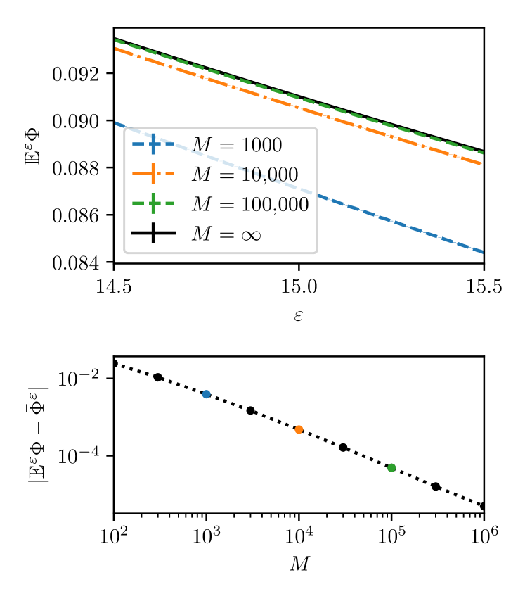
VI.2.2 The microscopic subsystems do not satisfy LRT but are appropriately heterogeneous

We consider a mean field coupled system of LRT-violating modified logistic maps (6). We choose the mean field coupling (8) and draw the parameters $a^{(j)}$ of the logistic map from the smooth raised-cosine distribution (9). In this case, the macroscopic dynamics $\Phi_{n}$ converges to a stable fixed point $\Phi_{n}\to\bar{\Phi}$ for $\varepsilon<-0.075$. The associated linear response is clearly visible in Figure 11. In fact, as discussed in Section V.2.2, nonlinear third order response holds for the three times continuously differentiable raised cosine distribution (9). We remark that for $\varepsilon>-0.075$ the mean field exhibits nontrivial dynamics in the thermodynamic limit, and we observe a breakdown of LRT to be discussed in Section VI.3.

Figure 11: Response term $\mathbb{E}^{\varepsilon}\Psi$ for the modified logistic map (6) with mean field coupling (8). The parameters $a^{(j)}$ are drawn from the raised-cosine distribution (9). Error bars were estimated from $10$ realisations of $10^{5}$ iterates, differing in the initial conditions of the heat bath, and are not visible.

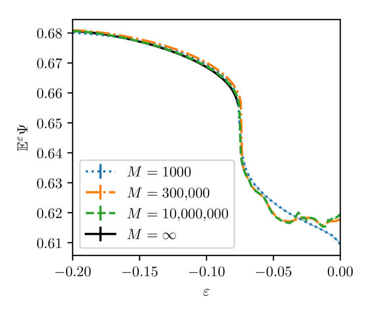
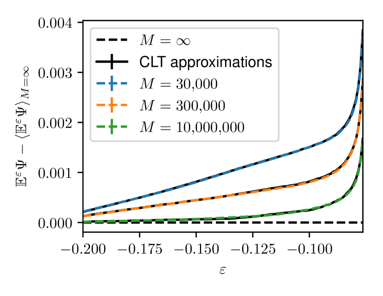
In Figure 12 we see very slow convergence of the mean $\mathbb{E}^{\varepsilon}\Psi$ to its limiting value: in particular, it is slower than the $\mathcal{O}(1/M)$ rate for uniformly expanding dynamics leading to trivial dynamics (cf Figure 10), and seemingly slower still than the $\mathcal{O}(1/\sqrt{M})$ rate that we might expect from sampling errors of $\eta$. Although smooth families of microscopic logistic maps allow for linear response of macroscopic observables to constant-in-time perturbations as discussed in Section V.2.2, and in fact numerical experiments (not shown) suggest that the susceptibility function $\chi$ has summable decay, they do not appear to have linear response with respect to stochastic perturbations. We argue that this counter-intuitive lack of linear response with respect to the (self-generated) stochastic perturbations arises from the noise-induced destruction of narrow periodic windows that have “extreme” values of $\mathbb{E}^{a,\varepsilon}\psi(q)$ compared with the neighbouring, more stochastically stable chaotic parameters. Thus at these periodic parameter values the macroscopic dynamics exhibits a disproportionately large response to the introduction of noise. We illustrate this in Figure 13, where we plot the response of a single logistic map with additive noise of variance $\sigma^{2}$. Here the noise models the finite size effects of the heat bath with $\sigma\sim 1/\sqrt{M}$. One sees clearly that periodic windows can be destroyed by very small amounts of noise ($\sigma=10^{-6}$). One also sees that associated with the destruction of these periodic windows is a very large response in the average $\mathbb{E}^{a}\psi$.

The statistical properties of the macroscopic observable for dynamics of a finite size heat bath can be modelled again by a surrogate system. Writing

$$\Phi_{n}=\bar{\Phi}^{\varepsilon,M}+\frac{1}{\sqrt{M}}\zeta_{n},$$

where $\zeta_{n}$ is the Gaussian CLT correction term to $\Phi_{n}\equiv\bar{\Phi}^{\varepsilon,\infty}$ with covariance given by (24). The macroscopic dynamics (30) then becomes

$$0=\mathbb{E}F(\bar{\Phi}^{\varepsilon,M}+\frac{1}{\sqrt{M}}\zeta_{n-1},\bar{\Phi}^{\varepsilon,M}+\frac{1}{\sqrt{M}}\zeta_{n-2},\ldots)-\bar{\Phi}^{\varepsilon,M}.$$

The response $\mathbb{E}^{\varepsilon}\Psi$ for this surrogate macroscopic dynamics is shown in Figure 12, labelled CLT approximation, and is barely distinguishable from the response of the original macroscopic dynamics.

Figure 12: Difference between the response term $\mathbb{E}^{\varepsilon}\Psi$ for finite $M$ and for the thermodynamic limit for the modified logistic map (6) with mean field coupling (8). The parameters $a^{(j)}$ of the logistic map are drawn from the raised-cosine distribution (9). For each value of $M$ the response of the corresponding CLT approximation using noise estimated from $M=10^{6}$ was used. Error bars were estimated from $10$ realisations of $10^{5}$ iterates, differing in the initial conditions of the heat bath, and are not visible.

Figure 13: Response term $\mathbb{E}^{a}\psi$ for a single stochastically driven logistic map $q_{n+1}=aq_{n}(1-q_{n})+\sigma\xi_{n}$, where $\xi_{n}$ is i.i.d. Gaussian noise and the observable $\psi(q)=q$. The response is recorded at increments of $da=10^{-8}$, thus for small $\sigma$ only a subset of narrow periodic windows are captured.

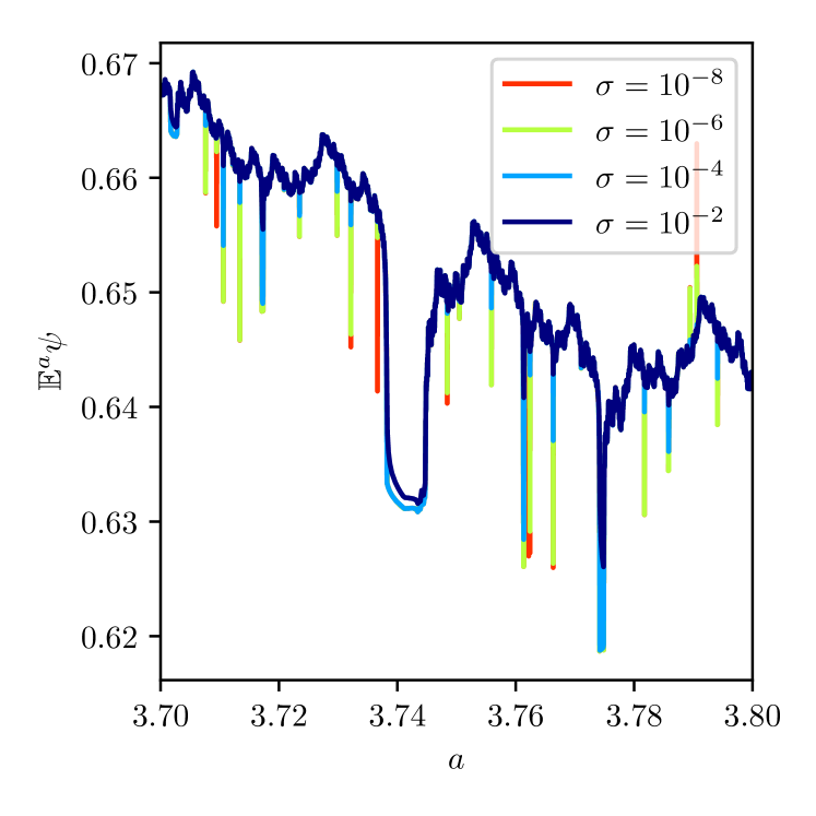
VI.2.3 The microscopic subsystems do not satisfy LRT and are not appropriately heterogeneous

For non-smooth distributions of the logistic map parameters $a^{(j)}$ such as the discrete distribution (10), the dynamics also converges to a stable fixed point $\bar{\Phi}^{\varepsilon,M}$ for $\varepsilon<-0.075$. The mean field $\bar{\Phi}^{\varepsilon,M}$ varies smoothly with respect to $\varepsilon$ for almost all $\varepsilon$, but $\mathbb{E}^{\varepsilon}\Psi$ experiences saddle node bifurcations on increasingly dense sets as $M$ approaches the thermodynamic limit $M\to\infty$. This is illustrated in Figure 14. Looking at (31), we see that linear response is violated where the fixed point loses stability and $\partial F(\bar{\Phi}^{\varepsilon},\bar{\Phi}^{\varepsilon},\cdots)/\partial\bar{\Phi}^{\varepsilon}=R(1)=1$.

For finite $M$, the macroscopic equation can be modelled as $\Phi_{n}^{\varepsilon,M}=\bar{\Phi}^{\varepsilon,M}+\zeta_{n}/\sqrt{M}$ where

$$\bar{\Phi}^{\varepsilon,M}=\mathbb{E}^{\varepsilon}F(\Phi_{n}^{\varepsilon,M},\Phi_{n}^{\varepsilon,M},\cdots).$$

The derivatives $\partial\mathbb{E}^{\varepsilon}F(\Phi_{n}^{\varepsilon},\Phi_{n}^{\varepsilon},\cdots)/\partial\bar{\Phi}^{\varepsilon}$ are well defined and thus for appropriate bath sizes $M$ we observe again approximate LRT for all practical purposes. However, as $M\to\infty$, saddle-node bifurcations become visible as a result of the diminishing effect of stability-providing noise, and in the thermodynamic limit we observe failure of LRT (see inset in Figure 14). The failure of linear response through saddle-node bifurcations is accompanied by $\mathbb{E}^{\varepsilon}\Psi$ experiencing multistability, with multiple very close stable equilibria, demonstrated in Figure 14. This can be understood as coming from the fact that $\mathbb{E}^{\varepsilon}F(\Phi_{n}^{\varepsilon,M},\Phi_{n}^{\varepsilon,M},\cdots)$ is essentially a smoothed out version of the rough logistic map response $\mathbb{E}^{\varepsilon}F(\bar{\Phi},\bar{\Phi},\cdots)$: as $M\to\infty$ the smoothing decreases, leading to increasing numbers of roots of the equation.

Figure 14: Response term $\mathbb{E}^{\varepsilon}\Psi$, including multistability, for the modified logistic map (6) with mean field coupling (8). The parameters $a^{(j)}$ are drawn from the discrete distribution (10). Error bars were estimated from $200$ realisations differing in the initial conditions (including initialising distributions) of the heat bath, and are not visible. The inset illustrates the occurrence of saddle-node bifurcations in the infinite-dimensional limit.

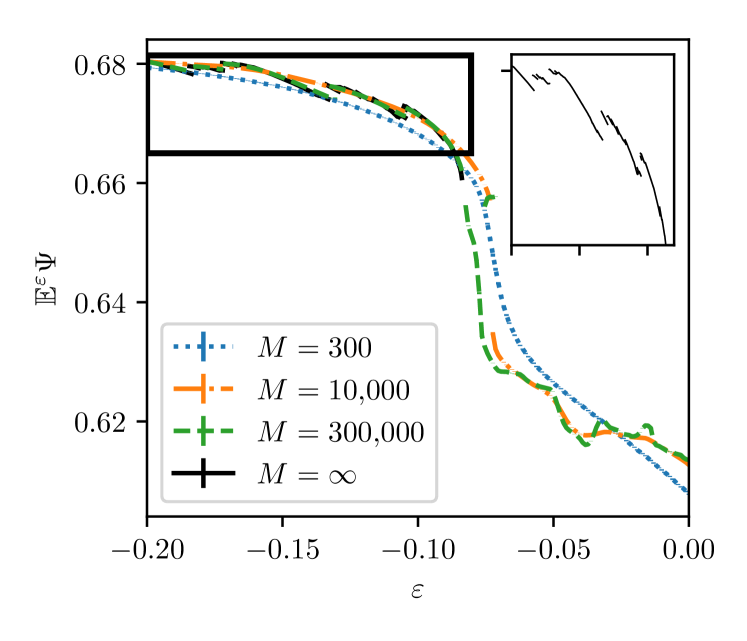
VI.3 Nontrivial dynamics of the mean field observable

The mean field $\Phi$ or any macroscopic observable $\Psi$ may itself exhibit non-trivial dynamics of varying complexity in the thermodynamic limit $M=\infty$. The overall response behaviour is then determined by the macroscopic dynamics rather than by the properties of the microscopic subsystems. We show the emergence of non-trivial chaotic macroscopic dynamics which violates LRT. The first one, surprisingly, involves a heat bath which evolves under uniformly expanding dynamics when uncoupled, and the second one involves microscopic dynamics that individually violate LRT.

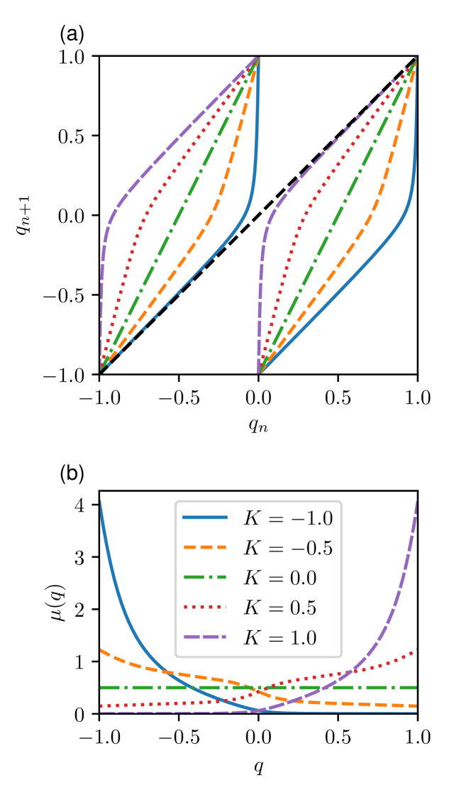
To generate emergent nontrivial macroscopic dynamics of the mean field, we again use the uniformly expanding map (32) with the even Lebesgue-measure zero coupling function $\phi(q)=-\tfrac{23}{30}+\tfrac{7}{2}q^{2}-2q^{4}$ to generate the mean field $\Phi_{n}$. We show in Figure 15 the map and its invariant measure, where the dynamics in the thermodynamic limit $M=\infty$ was computed using a spectral method Wormell (2019, ) (see Appendix B for more details). The map and coupling function $K_{n}$ are judiciously chosen to yield nontrivial dynamics for the mean field $\Phi_{n}$, mediating dynamics akin to a unimodal map for $\Phi_{n}$.

The map is constructed such that when the $q^{(j)}$ are approximately evenly distributed, $\Phi_{n}\approx 0$, causing an extreme value $K_{n}\approx\tanh(-2)\approx-0.96$: this pushes the $q^{(j)}$ strongly towards $q=-1$ which leads to a larger value $\Phi_{n+1}$, concentrating around $\Phi=2/\varepsilon$. For these values of $\Phi_{n+1}$, $K_{n+1}\approx 0$, and thus in the next step the $q^{(j)}$ are spread more evenly over the interval $[-1,1]$, mapping $\Phi_{n+1}$ back around zero. The concentration in the first step provides the folding and the sensitivity of $K_{n}$ to small changes in $\Phi_{n}$ for large $\varepsilon$ provides the stretching necessary for chaotic dynamics.

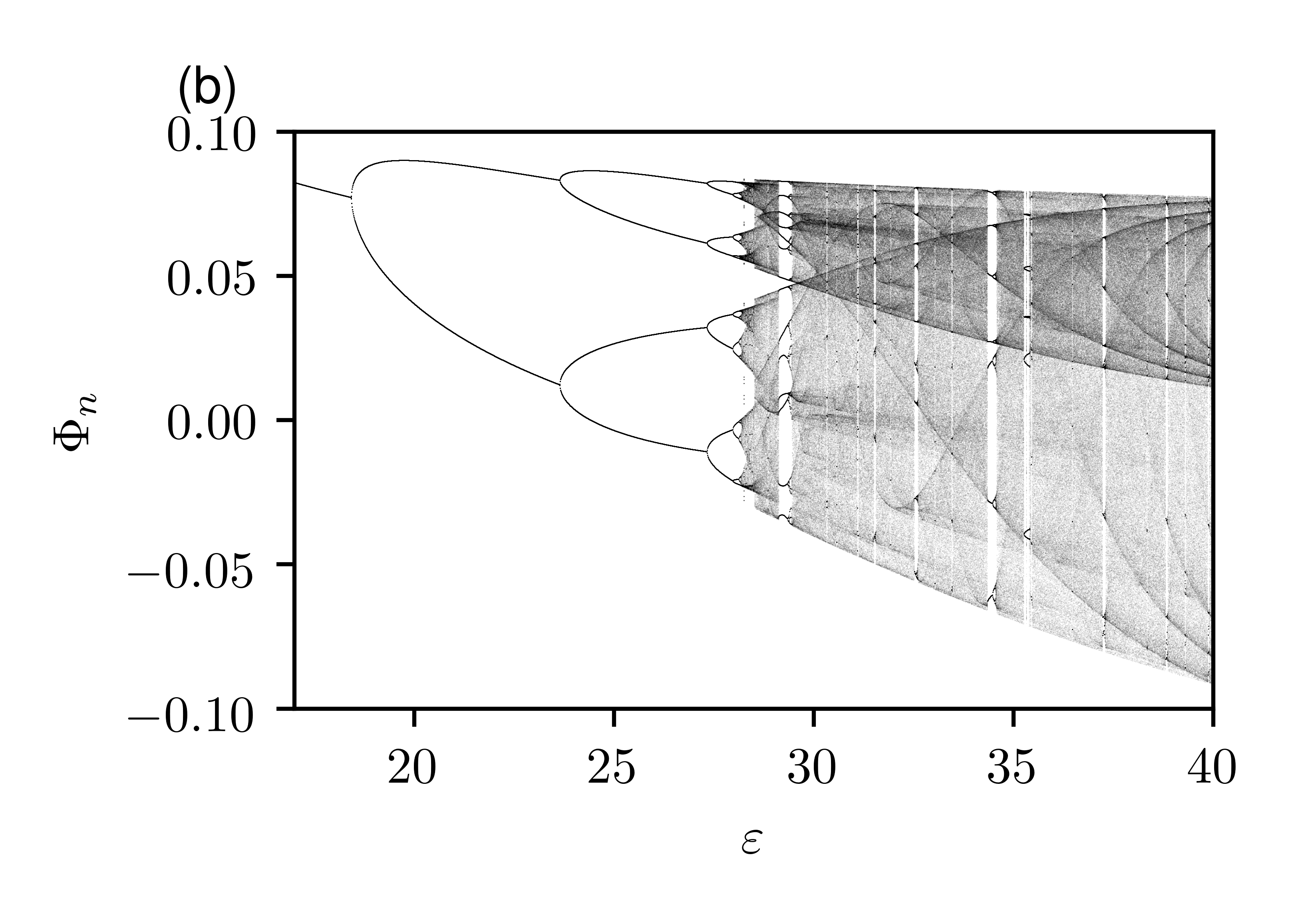
In Figure 16 we show the map $\Phi_{n+1}=F(\Phi_{n},\Phi_{n-1},\ldots)$ generated by the dynamical system (32) in the thermodynamic limit $M=\infty$ for $\varepsilon=30$. The dynamics is clearly chaotic with the leading Lyapunov exponent $\lambda_{1}=0.18>0$ ($\lambda_{2}=-0.43$ and $\lambda_{3}=-0.81$). The dynamics of the macroscopic observable $\Psi_{n}=\Phi_{n}$ exhibits a complex bifurcation cascade upon varying $\varepsilon$, depicted in Figure 16. For $\varepsilon\leq 18.4159$, the macroscopic dynamics has a stable fixed point; upon increasing the perturbation $\varepsilon$ a period-doubling cascade leads to chaotic, apparently unimodal-like, dynamics intermingled with periodic windows for values of $\varepsilon>26.1649$. One can clearly see dark scars in the bifurcation diagram in the chaotic region of $\varepsilon>26.1649$. This is reminiscent of the logistic map Collet and Eckmann (2007) where the scars denote narrow intervals of $\langle\Phi_{n}\rangle$ with increased probability, corresponding to large spikes in the invariant measure, which (unlike small spikes) vary smoothly with respect to perturbations $\varepsilon$.

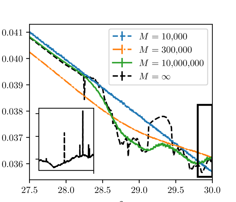
In Figure 17 we show the linear response term $\mathbb{E}^{\varepsilon}\Psi$ of the uniformly expanding map (32) for several finite $M$ heat bath sizes and for the thermodynamic limit $M=\infty$ for $\varepsilon\in[27.5,30]$, clearly illustrating the breakdown of LRT. We recall that the same map exhibits LRT for small values of $\varepsilon$, where the macroscopic mean field converges to a stable fixed point, for the same parameters (cf. Figure 10).

Figure 15: (a) Plot of the uniformly expanding map (32) and (b) its invariant measure for various values of $K_{n}\equiv K$.

Figure 16: (a): 2D projection of the attractor onto delay coordinates of the macroscopic map $\Phi_{n+1}=F(\Phi_{n},\Phi_{n-1},\ldots)$ generated by the uniformly expanding map (32) for $\varepsilon=30$. The system has two periodic components separated by a gap around the unstable fixed point $\Phi_{n-k}\equiv 0.51258$. (b): Bifurcation diagram of the map (32) showing period doubling bifurcations and chaotic dynamics.

Figure 17: Response term $\mathbb{E}^{\varepsilon}\Psi$ of the uniformly expanding map (32) for finite $M$ response, showing convergence to the thermodynamic limit $M\to\infty$. The black box shows the region which is magnified on the right. Error bars were estimated from $10$ realisations differing in the initial conditions of the heat bath, and are not visible.

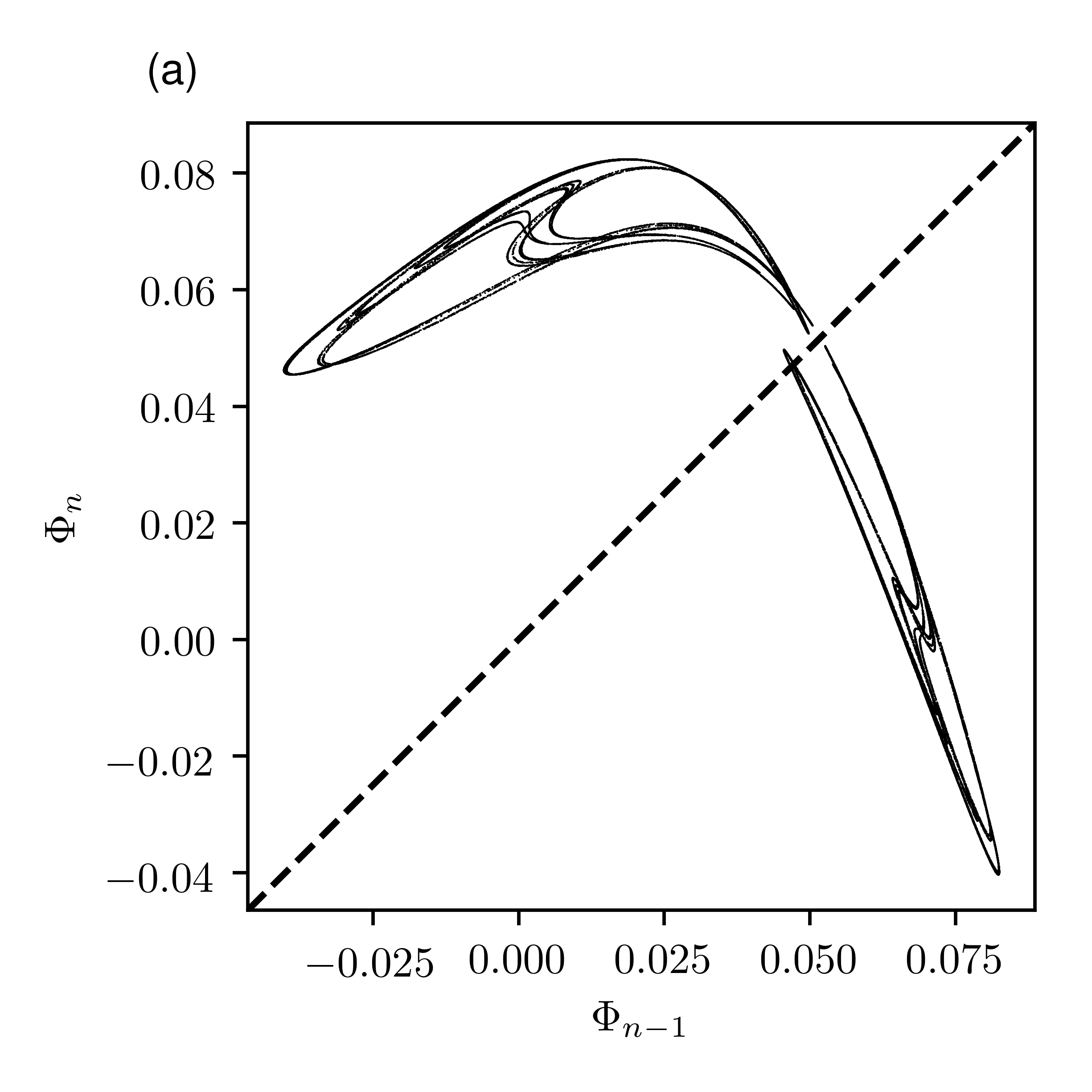
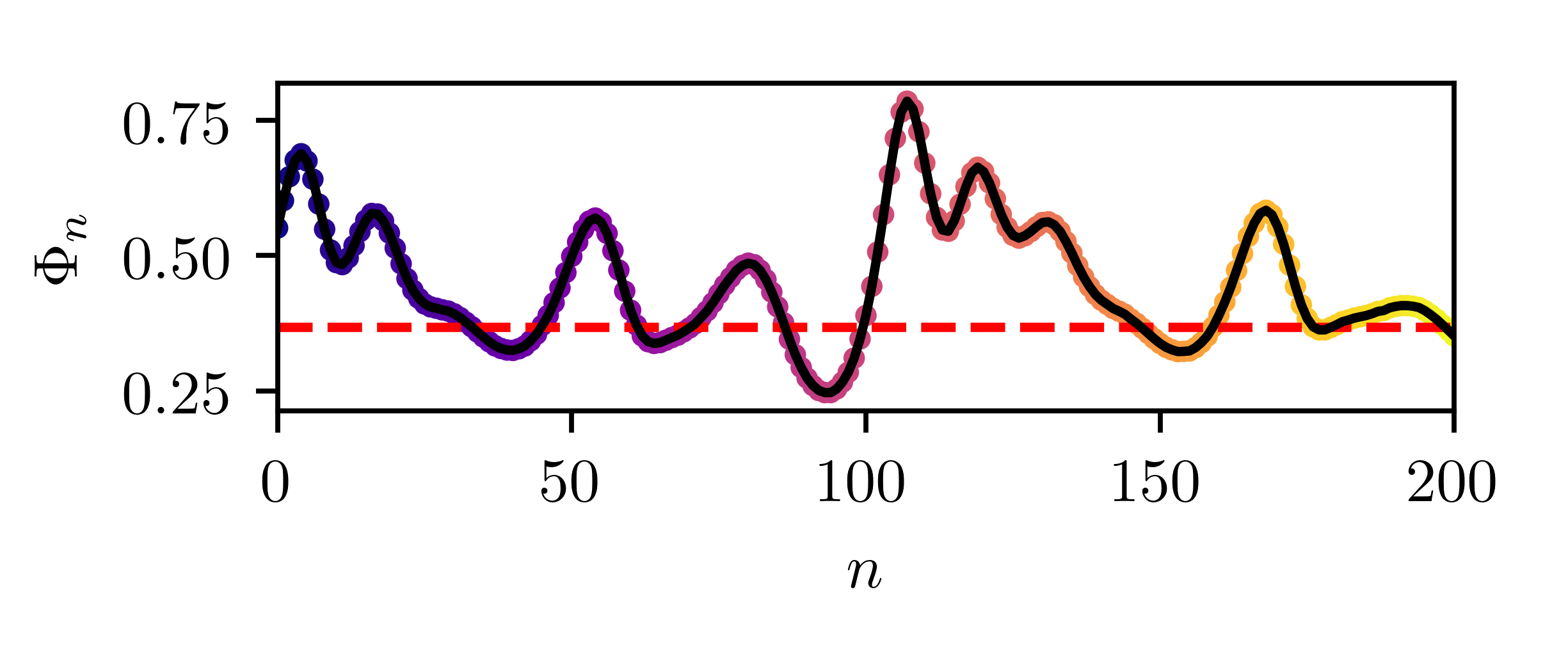
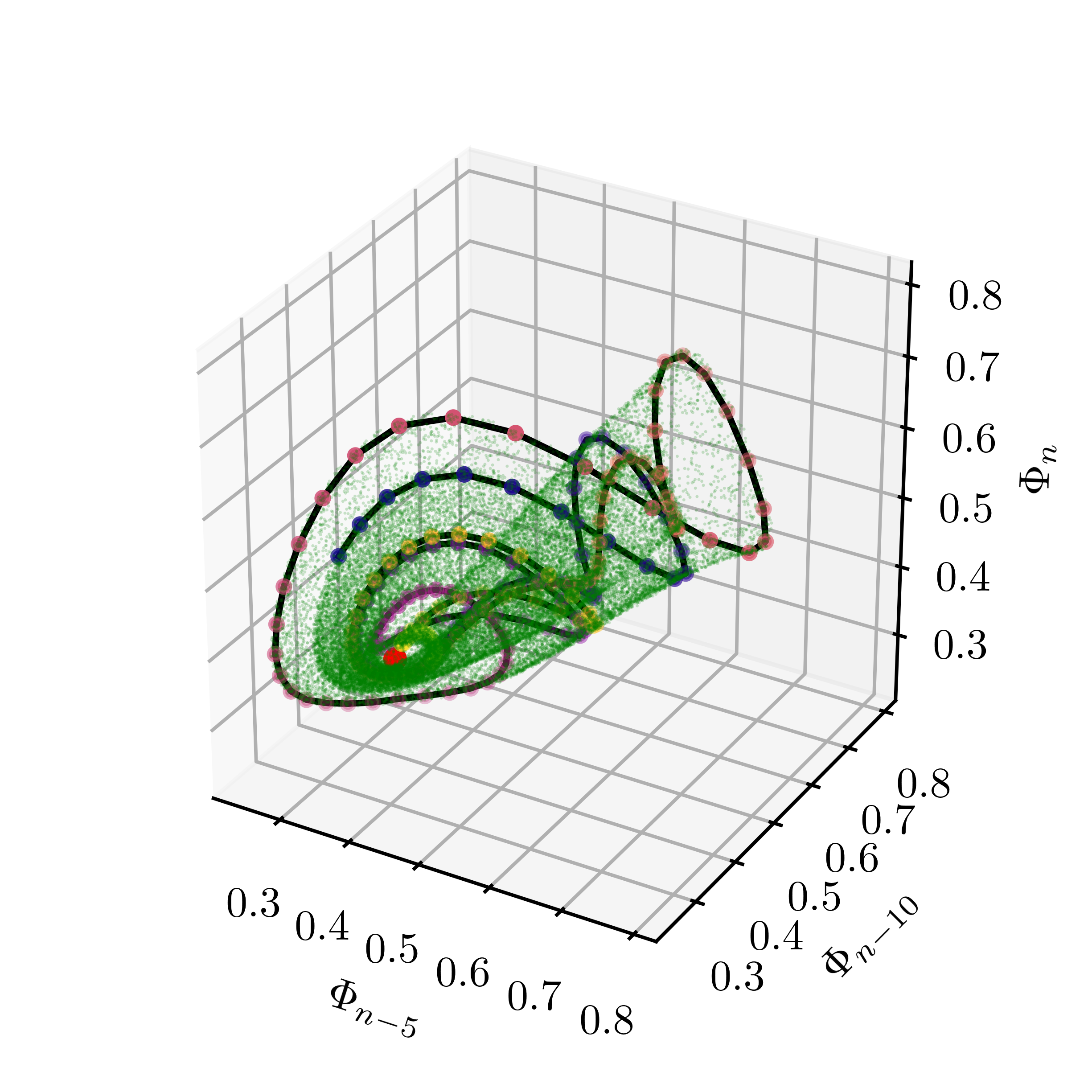
For curiosity and to further study the effect of the self-generated noise on the LRT behaviour of macroscopic observables in the mean field coupled case, we provide another example of nontrivial chaotic mean field dynamics which violates LRT. We revisit the mean field coupled dynamics of microscopic subsystems which do not satisfy LRT discussed in Section VI.2.2, and consider the modified logistic map (6) with mean field coupling (8) where the parameters $a^{(j)}$ of the logistic map are drawn from the smooth raised-cosine distribution (9). We recall that for $\varepsilon\approx[-0.2,-0.075]$ the macroscopic dynamics (29) was trivial and $\mathbb{E}^{\varepsilon}\psi$ satisfies LRT (cf. Figure 11). The stable fixed point loses stability at $\varepsilon\approx-0.075$ through a saddle-node bifurcation (not shown), from which emanates a stable limit cycle centred around an unstable fixed point with $\mathbb{E}\Psi\approx 0.615$: as $\varepsilon$ increases, this bifurcates to chaos and for a wide range of values $\varepsilon>-0.075$ nontrivial chaotic macroscopic dynamics of (29) is observed. Figure 18 illustrates the macroscopic dynamics for $\varepsilon=0$, which exhibit Shilnikov-type chaos. The associated response term $\mathbb{E}^{\varepsilon}\Psi$ was shown in Figure 11 for several finite heat bath sizes $M$ and for the thermodynamic limit $M=\infty$ for $\varepsilon\in[-0.2,0]$, clearly illustrating the transition to LRT violating macroscopic dynamics around $\varepsilon=-0.075$. Note that the finite size response is smoothed due to the self-generated noise process $\zeta_{n}$.

The examples given above of high-dimensional system exhibiting non-uniformly hyperbolic chaotic collective behaviour are in disagreement with the often invoked assumption that macroscopic observables of high-dimensional systems obey linear response. This is the more surprising as the non-uniformly hyperbolic chaotic behaviour is robust (modulo periodic windows) with respect to the external perturbation, different choices of the coupling function, different weightings in the coupling, etc.

Figure 18: Top: Time series of the macroscopic map $\Phi_{n+1}=F(\Phi_{n},\Phi_{n-1},\ldots)$ generated by the modified logistic map (6) with mean field coupling (8) for $\varepsilon=0$, approximated by a finite ensemble of size $M=10^{7}$. The red dotted line shows an unstable fixed point of the system. The parameters $a^{(j)}$ are drawn from the raised-cosine distribution (9). Bottom: Projection onto delay coordinates of the attractor and dynamics of the same map. The red dot near the centre of the attractor denotes an unstable fixed point of the system.

VII Discussion

We established conditions under which macroscopic mean field observables enjoy linear response. We considered two scenarios, macroscopic observables of an uncoupled collection of microscopic subunits as well as macroscopic observables of microscopic subunits which are coupled via their mean field. We found that linear response is possible even in the case when the microscopic systems individually violate LRT, provided the microscopic dynamics is heterogeneous with parameters drawn from a sufficiently smooth distribution. We also found that for back-coupled systems of finite size, LRT (for small enough perturbations) is expected for any kind of microscopic dynamics: this can be understood as the result of emergent, self-generated stochastic effects. We further established that in the thermodynamic limit of infinite $M$, the mean field dynamics can exhibit attracting dynamics that appears non-uniformly hyperbolic and certainly fails to have LRT, even when the microscopic subunits are individually uniformly expanding; this presents a counter example to the widely believed hypothesis that macroscopic observables of high-dimensional systems typically obey linear response.

Our results rely on the existence of statistical limit laws such as the central limit theorem. These are proved for strongly chaotic systems, and in particular for uniformly expanding maps as well as for smooth unimodal maps. We follow here Gottwald and Melbourne (2014) and assume that typical dynamical systems are strongly chaotic and hence enjoy good statistical properties, so that our results carry over to typical dynamical microscopic systems. To ensure the existence of the CLT and the convergence of the deviations $\zeta_{n}$ to a Gaussian process with decay of correlations, we require the observables $\psi(q)$ to be at least Hölder continuous and the external forcing $\varepsilon$ to be such that the perturbed system is mixing.

We presented here results for mean field observables $\Psi$ of the form (2). We remark that our results carry over for more general (e.g. weighted) mean field variables provided those weights are sufficiently smoothly distributed, and indeed we expect broadly similar results for more general “macroscopic” observables.

In previous work on LRT in high-dimensional systems we considered the more specific case where $\varepsilon$ was an additive perturbation of the logistic parameters $a^{(j)}$Wormell and Gottwald (2018). The case of homogeneous additive perturbations can be applied to the macroscopic observables treated here. This is readily seen, e.g. in the uncoupled case, by writing

$$\langle\mathbb{E}^{\varepsilon}\Psi_{n}\rangle =\iint\psi(q)d\mu^{{a+\varepsilon}}_{n}(q)d\nu(a)$$

$$=\iint\psi(q)d\mu^{{a}}_{n}(q)\nu(a-\varepsilon)da.$$

The linear response term is then readily evaluated as

$$\frac{d}{d\varepsilon}\langle\mathbb{E}^{\varepsilon}\Psi_{n}\rangle =-\iint\psi(q)d\mu^{{a}}_{n}(q)\frac{d}{da}\nu(a)da,$$

which implies that LRT is valid provided that the system is appropriately heterogeneous with integrable distribution $d\nu(a)/da$.

To reduce the complexity of expression we have enforced mixing dynamics, with no chaotic synchronisation, for example by including the hidden $r$-dynamics in (6). It would be interesting to study the case when the microscopic dynamics is not restricted in this way, for example if periodic dynamics were allowed. We have only discussed the existence of LRT and have not considered fluctuation-dissipation formulae to provide a compact analytical formula for the response term. This may require treatment of the non-Markovian dynamics of the macroscopic variable as well as the interplay of the perturbed microscopic dynamics and the macroscopic dynamics, the latter having been studied in the context of slow-fast systemsAbramov (2010).

We have corroborated our findings with detailed numerical simulations and have provided several heuristic arguments based on statistical limit laws: we hope these arguments can be made rigorous. We remark that in the case of uncoupled systems, rather than averaging over the heat bath, one may express the invariant measures $\mu^{(a_{j}}$ as an infinite sum over the systems’ unstable periodic orbits (UPOs) Ruelle (2004); Pollicott (1986); Cvitanovic and Eckhardt (1991); Eckhardt and Grossmann (1994). This approach may be more effective when trying to rigorously justify the convergence of the deviations $\zeta_{n}$ to a Gaussian process. It seems likely also possible to apply ideas from a recent argument by Ruelle for linear response in non-hyperbolic systems, based on the statistical smearing-out of singularities in the physical measuresRuelle (2018).

Appendix A Statistical test for linear response given time series

A statistical test to probe the linear or higher-order response of a chaotic system from time series data at various parameter values was proposed in Gottwald, Wormell, and Wouters (2016). In this appendix we summarise the principles of this test, which we use in the body of this paper.

Suppose that a system has response $\mathbb{E}^{\varepsilon}\Psi$ which has certain regularity properties for $\varepsilon\in[\varepsilon_{1},\varepsilon_{2}]$ (or around some $\varepsilon_{0}$), and suppose this regularity property means that there exist functions $\varphi_{i}(\varepsilon),i=1,\ldots,I$ and (unknown) coefficients $\beta_{i}\in{\mathbb{R}}$ such that

$$\mathbb{E}^{\varepsilon}\Psi\approx\sum_{i=1}^{I}\beta_{i}\varphi_{i}.$$ (33)

is a good approximation in $L^{2}([\varepsilon_{1},\varepsilon_{2}])$.

For example, if $\mathbb{E}^{\varepsilon}\Psi$ is $C^{1}$ and $\varepsilon_{2}-\varepsilon_{1}$ is sufficiently small, then $\mathbb{E}^{\varepsilon}\Psi$ can be well-approximated with a Taylor expansion about $\varepsilon_{1}$: thus, $\varphi_{0}\equiv 1$ and $\varphi_{1}(\varepsilon)=\varepsilon-\varepsilon_{1}$ form a good basis for approximation, and we would expect an $L^{2}$ error of size $o(\varepsilon_{1}-\varepsilon_{2})$. If instead $\mathbb{E}^{\varepsilon}\Psi$ is smooth (e.g. $C^{r}$) on a larger interval, then we could choose Chebyshev polynomials as a basis for approximation $\varphi_{i}(\varepsilon)=T_{i-1}((2\varepsilon-\varepsilon_{1}-\varepsilon_{2})/(\varepsilon_{2}-\varepsilon_{1}))$ for $i=1,\ldots,I$, with an $L^{2}$ error of $O(I^{r})$.

Suppose that for perturbation values $\varepsilon_{j},\,j=1,\ldots,J$ we have time series of the observable’s dynamics $(\Psi_{j,n})_{n=1,\ldots,N}$ where the time series length $N$ is sufficiently large. Supposing that (as is typical for many systems Gottwald and Melbourne (2013)) $\Psi_{n}$ obeys a CLT for each selected parameter, then for large enough $N$ the Birkhoff averages for each $\varepsilon_{j}$ have Gaussian approximations

$$\bar{\Psi}^{N}_{j}:=\frac{1}{N}\sum_{j=1}^{N}\Psi_{j,n}=\mathbb{E}^{\varepsilon_{j}}\Psi+\sigma(\varepsilon_{j})\xi_{j}/\sqrt{N},$$ (34)

where $\xi_{j}$ are i.i.d. standard normal variables and the Birkhoff variance $\sigma^{2}(\varepsilon_{j})$ can be estimated by various means, including taking multiple time series for each $\varepsilon_{j}$, or subsampling.

If we define the vector with coefficients $y_{j}=\bar{\Psi}^{N}_{j}$ and the matrix with coefficients $X_{ji}=\sqrt{N}\sigma(\varepsilon_{j})^{-1}\varphi_{i}(\varepsilon_{j})$, then we can write (33-34) as the linear equation

$$y=X\beta+\xi,$$

where $\xi\sim\mathcal{N}(0,I_{J\times J}).$ This is of course just a standard linear statistical model, and we can use the theory of these modelsRice (2006) to test the null hypothesis that the approximation of the response by the $\phi_{i}$ (33) is an equality, i.e. that $\mathbb{E}^{\varepsilon}\Psi$ has linear (or smooth) response.

Defining the least-squares projection matrix

$$H=X(X^{T}X)^{-1}X^{T}$$

and the Pearson chi-square test statistic

$$\chi^{2}=y^{T}(I-H)y,$$

we have that if the approximate equality in (33) is exact, then $\chi^{2}$ has chi-squared distribution $\chi^{2}_{J-I}$ where $I$ is the number of basis functions $\varphi_{i}$.

If $\chi^{2}_{\textrm{obs}}$ is the observed value of the test statistic, the p-value for the test for linear (or higher-order) response is then given by

$$p=P(\chi^{2}_{J-I}\geq\chi^{2}_{\textrm{obs}}),$$

provided the error associated with the non-exact nature of the approximation (33) is appropriately small. This error is small if

$$\mathbb{E}\chi^{2}-\mathbb{E}\chi^{2}_{J-I}=N\|(I-H)(\mathbb{E}^{\varepsilon_{j}}\Psi/\sigma(\varepsilon_{j}))_{j=1,\ldots,J}\|_{\ell^{2}},$$

which, supposing $\sigma$ is a reasonably smooth function of $\varepsilon$ and the $\varepsilon_{j}$ are uniformly spaced, estimates the minimum possible $L^{2}(\sigma^{2})$ error in approximations of the response of the form in (33), multiplied by the sample sizes $N$.

Appendix B Numerical method to compute the thermodynamic limit $M\to\infty$ for uniformly expanding maps

In the thermodynamic limit of infinite $M$ the strong law of large numbers holds and

$$\Phi_{n}=\langle\mathbb{E}\Phi_{n}\rangle=\int\phi(q)d\mu_{n}(q),$$

where $\mu_{n}$ is the (time-varying) physical measure of the system, which evolves as

$$\mu_{n+1}=\mathcal{L}_{K_{n}}\mu_{n},$$

where $\mathcal{L}_{K_{n}}$ is the transfer operator of the system (32) and recalling that $K_{n}=\tanh(\varepsilon\Phi_{n}-2)$.

Because for all fixed $K_{n}=K$ the map (32) is uniformly expanding, the physical measures $\mu_{n}$ are absolutely continuous with respect to Lebesgue, and we can write them as $\mu_{n}(q)dq$. Furthermore, because the map (32) is analytic and hence infinitely many times differentiable, it is possible to approximate the measure density and transfer operator dynamics very accurately using Chebyshev spectral Galerkin methods Wormell (2019). We have implemented an adaptive-order spectral approximation of the measure density in the Julia package Poltergeist.jl Wormell , which allows us to simulate the dynamics of $\mu_{n}$. The core routine, which outputs $\mu_{n+1}$ and $\Phi_{n+1}$ given inputs $\mu_{n}$, $\varepsilon$ and the driving $d_{n}$ (by default $\Phi_{n}$), is defined as follows (note that Julia recognises Unicode characters):

⬇

function F($\mu$_n, $\varepsilon$, d_n = sum($\phi$*$\mu$_n))

K_n = tanh(d_n*$\varepsilon$-2)

f_n = f_map(K_n)

# create MarkovMap object

$\mu$_n1 = transfer(f_n,$\mu$_n)

# compute $\mu_{n+1}$

return $\mu$_n1, sum($\phi$*$\mu$_n1)

end

More details of the algorithm and some examples of its use may be found at https://github.com/wormell/PoltergeistExamples/blob/master/WeakSelfCoupling-LimitingSystem.ipynb.

After the first time the routine is called (during which Julia compiles the code), the algorithm takes around $8\times 10^{-4}$ seconds on a standard laptop to compute each $\mu_{n+1}$ from $\mu_{n}$, and has an approximation error of only around $10^{-13}$: by comparison, if one aims to estimate $\mu_{n}$ as a Monte-Carlo approximation with a large ensemble of $M=\mathcal{O}(10^{8})$, a relatively large approximation error of $10^{-3}$ is incurred.