Use and implementation of autodifferentiation in tensor network methods with complex scalars

Abstract

Following the recent preprints arXiv:1903.09650 and arXiv:1906.04654 we comment on the feasibility of implementation of autodifferentiation in standard tensor network toolkits by briefly walking through the steps to do so. The total implementation effort comes down to less than 1000 lines of additional code.

We furthermore summarise the current status when the method is applied to cases where the underlying scalars are complex, not real and the final result is a real-valued scalar. It is straightforward to generalise most operations (addition, tensor products and also the QR decomposition) to this case and after the initial submission of these notes, also the adjoint of the complex SVD has been found.

1 Introduction

Autodifferentiation (AD) is a technique to automatically compute the gradient of a computer program by defining the partial derivatives of the individual building blocks of the program and then using the chain rule to combine the partial derivatives of the steps run during the computer program execution into an overall derivative. The method is a standard tool in the field of machine learning, where automatically computed gradients are used for the optimisation of neural networks (called “backpropagation”). It was recently by Liao et al[1] into the field of tensor network methods in the context of infinite projected entangled pair states and has already been applied to other problems as well[2].

Here, we want to firstly demonstrate that the implementation of reverse-mode autodifferentiation is straightforward in a standard tensor networks toolkit as typically used in the community without relying on existing toolchains such as TensorFlow or PyTorch. Such a “native” implementation has the advantage of exploiting all the standard tricks to speed up condensed-matter simulations, in particular the use of symmetries[3, 4, 5, 6, 7, 8, 9, 10, 11] to enforce a block structure on tensors.

Secondly, we want to summarise the current status when the scalars employed in the tensor network intermittently are not real but complex (e.g. std::complex<double> instead of double), with only the final result, such as an energy or cost function, being real-valued again.

2 Implementation Effort for Reverse-Mode AD

While the authors have implemented reverse-mode AD in the SyTen[12] tensor networks toolkit, the implementation can likely proceed in much the same way in any other codebase. The STensor class introduced into the SyTen toolkit in 2018 provides named tensor indices, automatic tensor products over equal-named indices, automatic handling of fermionic indices without the need for swap gates[13, 14] and can be combined with an AsyncCached<> template to transparently and asynchronously cache tensor contents to disk when not needed.

Implementation of autodifferentiation support proceeded in two steps:

2.1 ComputeNode history storage

The STensor class was extended by two objects: an autodifferentiation ID, uniquely identifying the specific tensor object, and a shared pointer to a ComputeNode object. The ComputeNode class represents a particular step of a calculation, e.g. an addition or tensor-tensor product. Each ComputeNode stores a list of shared pointers to the compute nodes associated with the input tensors of the operation, a list of IDs of the output tensors generated (typically 1, but e.g. the QR decomposition produces two output tensors), an adjoint evaluation function and cached copies of the tensors necessary for the adjoint evaluation function to run. It was useful to also store empty tensors of the shape of the output tensors (and hence output adjoints) to more generally handle cases where these adjoints may be zero due to the result not depending on that particular output.

When enabling autodifferentiation on a specific tensor, an initial compute node is created for this tensor. Tensor operations create subsequent compute nodes which build up a directed acyclic graph.

Once the desired result value is obtained, requesting the autodifferenation of this output value with respect to a valid autodifferentiation ID causes the graph to be traversed backwards until the compute node producing this ID is found. During this traversal, the graph is double-linked such that each node knows which other nodes rely on its output as an input. When the original node is found, its output adjoint with respect to the result value autodifferentiation ID is requested. This request percolates down the tree, each node first computing the adjoints of its outputs by requesting the adjoints of the inputs from its downstream nodes and those adjoints of inputs being evaluated by the associated adjoint evaluation function stored in each node.

For efficiency, the result of the output adjoint evaluation is cached in each node such that multiple differentials can be computed easily. For convenience and debugging, it is also possible to draw the directed acyclic graph representing the computation (in our case, by producing an input file to the ‘dot‘ program which handled the actual drawing). The overall framework including the definition of compute nodes, their clean-up and the calculation of adjoints (given the adjoint evaluation functions defined elsewhere) can be done in about 350 physical lines of C++.

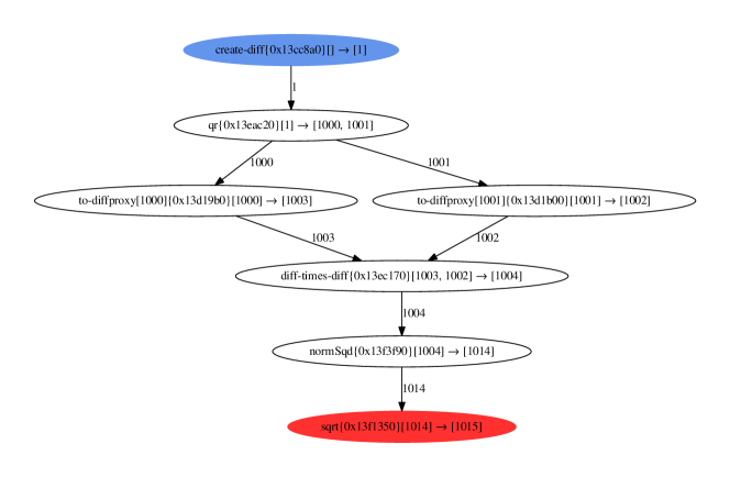
Figure 1: An exemplary computation tree resulting from the evaluation $Q,R=\mathrm{qr}(X);Y=Q\cdot R;Z=\sqrt{||Y||^{2}_{\mathrm{Frob}}}$. The tensor-tensor product takes two temporary proxy objects, here showing up as to-diffproxy operations.

2.2 Definition of AdjointEvaluator functions

Once the basic framework exists, one has to adapt every function manipulating an STensor object to potentially store its computation and adjoint evaluation function in a compute node, if that STensor object has autodifferentiation enabled. If one first changes every function to assert that its input tensors do not have autodifferentiation enabled the additional definitions can be added one by one without fear of introducing undetected errors.

In the following, we will consider some examples of such adjoint evaluation functions. These function should, when called from a compute node which has as input a tensor $I$ and produced a tensor $T$ with final scalar result $R$, evaluate the “input adjoint” $\frac{\partial R}{\partial I}$ where they can rely on $\frac{\partial R}{\partial T}$ being available as the “output adjoint” sum of the input adjoints of downstream nodes.

As a first example, consider a function which changes the name of one of the tensor legs, that is, $x_{\ldots,i,\ldots}\to f(x_{\ldots,i,\ldots}=x_{\ldots,j,\ldots}$. Working reverse, we need to change the tensor leg $j$ of the output adjoint back to have the name $i$. If the output adjoint has such a leg, this can be done simply by renaming. If it does not (typically not the case if the final result which we differentiate is a scalar), we need to take the outer product of the output adjoint and an identity tensor mapping $i$ to $j$.

Second, consider the case of a tensor-tensor addition $I_{1}+I_{2}=T$. The partial derivative $\partial T/\partial I_{1,2}$ is one, hence when the input adjoint with respect to either $I_{1}$ or $I_{2}$ is requested, we can simply return the output adjoint $\partial R/\partial T$. Note that neither of these two cases require storing either the input or output tensors of the node.

Third, consider the case of hermitiation conjugation, that is $X\to f(X)=X^{\dagger}$. For complex-valued scalars, it is easiest to assume that $\partial X^{\dagger}/\partial X$ is zero and hence simply discard all earlier history and consider the resulting tensor $X^{\dagger}$ as a potential new origin tensor. In the real-valued case, the situation is more complicated as $X^{T}$ does depend on $X$ and the adjoint evaluator has to return the transpose of the output adjoint it obtains from downstream. This can be seen by writing the transposition as a series of tensor-tensor products[15] with tensors of the form $\delta^{ii}$ or $\delta_{jj}$ to exchange upstairs and downstairs indices. The local partial derivative is then just those tensors, multiplying them into the output adjoint transposes it.

Fourth, the case of tensor-tensor products $I_{1}\cdot I_{2}=T$ can also be handled straightforwardly, however, now it is necessary to store both input tensors $I_{1,2}$. The adjoint evaluation simply has to multiply the downstream adjoint by either $I_{1}$ or $I_{2}$.

2.2.1 Tensor decompositions

For both the eigenvalue decomposition, the QR decomposition and the singular value decompositions, expressions for the adjoints in the real case are straightforwardly available[16, 17, 18, 1]. While implementing those operations, in particular the element-wise Hadamard products, is tricky, this can also be done. Note that the adjoints of these decompositions typically rely on matrix inversion (either of the singular value matrix, the eigenvalue matrix or the upper-triangular matrix in the QR), which may cause numerical problems unless stabilised[1].

3 Complex Scalars

The standard machine learning toolkits mostly handle the case of real-valued scalars. However, in quantum physics, complex scalars are not often avoidable. It is hence interesting to see how reverse-mode autodifferentiation applies to the case of complex scalars if the final result value $r$ is limited to the reals: That is, we consider tensor operations that take complex-valued input tensors and finally produce a real value, $f:\mathbb{C}^{n}\to\mathbb{R}$. This is for example the case where we wish to obtain the gradient of a physical observable (such as the energy) or if we otherwise want to optimise some cost function (e.g. entanglement over a bond). Naturally, the functions we consider are typically not analytic, i.e. depend on both the input variables $z$ and their complex conjugates $z^{\dagger}$. In those cases, it is most natural to consider $z$ and $z^{\dagger}$ to be independent variables and make use of the Wirtinger derivative

$$\frac{\partial}{\partial z}\equiv\frac{1}{2}\left[\frac{\partial}{\partial\mathrm{Re}(z)}-\mathrm{i}\frac{\partial}{\partial\mathrm{Im}(z)}\right]\;.$$ (1)

Evaluating $\frac{\partial r(Z,Z^{\dagger})}{\partial Z}$ for a complex tensor $Z$ and a real-valued scalar $r$ yields the gradient of $r(Z,Z^{\dagger})$ at position $Z$, its hermitian conjugate $\left(\frac{\partial r(Z,Z^{\dagger})}{\partial Z}\right)^{\dagger}$ is the conjugate gradient (which has the same dimensions as $Z$) and may be used to take a step in the direction of steepest ascent/descent. Note that

$$\left(\frac{\partial r(Z,Z^{\dagger})}{\partial Z}\right)^{\dagger}=\frac{\partial r(Z,Z^{\dagger})}{\partial Z^{\dagger}}\;.$$ (2)

See [19] for a pedagogical overview and further details.

3.1 Standard Operations

All standard operations such as addition, tensor products or index renaming translate straightforwardly from the real to the complex case and no special handling in code is required. Only taking the hermitian conjugate requires differentiating between the real and complex case – in the former, it is equivalent to a simple tensor transpose (which is differentiable), in the latter, it creates a new independent variable.

Functions which produce either the real or imaginary part of their inputs are best represented as additions/subtractions with the complex conjugate followed by multiplication by a scalar $\frac{1}{2}$ or $\frac{-\mathrm{i}}{2}$. The complex conjugate is an independent variable and hence does not matter, the multiplication by a scalar simply needs to be translated to the downstream adjoint.

3.2 QR Decomposition

While the available literature only discusses real QR decompositions, the complex QR decomposition is also unique if one requires the diagonal of $R$ to be real and positive. It is useful to insert a manual check to this end in the QR decomposition, depending on the underlying library/LAPACK implementation.

Thankfully, the calculation steps done to produce adjoints of $Q$ and $R$ in the real case translate straightforwardly to the complex case:

Let in the following $A_{i}^{j}$ denote elements of a matrix $A\in\mathbb{C}^{\dim(i)\times\dim(j)}$ with $\dim(i)\geq\dim(j)$ (“tall”). The element-wise complex conjugate of a matrix $X_{i}^{j}$ is given by $\underline{X}_{i}^{j}$. The QR decomposition of $A$ is given by matrices $Q\in\mathbb{C}^{\dim(i)\times\dim(x)}$ and $R\in\mathbb{C}^{\dim(x)\times\dim(j)}$ such that

$$A_{a}^{i} =Q_{a}^{x}R_{x}^{i}\;.$$ (3)

Furthermore $Q^{\dagger}Q=\mathbf{1}$, i.e.:

$$\underline{Q}^{x}_{a}Q_{a}^{{x^{\prime}}}\delta^{aa}=\delta^{x{x^{\prime}}}\;.$$ (4)

Furthermore, we have projectors $L_{\alpha}^{\beta}=1\textrm{ iff }\alpha>\beta$, $U_{\alpha}^{\beta}=1\textrm{ iff }\beta>\alpha$ and $D_{\alpha}^{\beta}=1\textrm{ iff }\alpha\equiv\beta$. With those projectors, the triangularity of $R$ is

$$R_{x}^{i}L_{x}^{i}=0_{x}^{i}\;.$$ (5)

3.2.1 Aim

The total differential of a real-valued function $\phi$ which we are interested in is (cf. [19], pg. 11)

$$\differential\phi=\frac{\partial\phi}{\partial A_{a}^{i}}\differential A_{a}^{i}+\frac{\partial\phi}{\partial\underline{A}_{a}^{i}}\underline{\differential A}_{a}^{i}=a^{a}_{i}\differential A_{a}^{i}+\underline{a}^{a}_{i}\underline{\differential A}_{a}^{i}$$ (6)

with the adjoint $a$ the prefactor of $\differential A$ in $\differential\phi$, of which we want to take twice the real part. Because the adjoint of $\underline{A}$ is equal to the complex-conjugate of the adjoint of $A$ for real-valued $\phi$, we can choose to either evaluate $a$ and complex-conjugate it or evaluate $\underline{a}$ directly. In any case, $\underline{\differential A}$ is only the complex conjugate of $\differential A$.

Written in terms of $Q$ and $R$, this is

$$\differential\phi=q_{x}^{a}\differential Q_{a}^{x}+r_{i}^{x}\differential R_{x}^{i}+\underline{q}_{x}^{a}\underline{\differential Q}_{a}^{x}+\underline{r}_{i}^{x}\underline{\differential R}_{x}^{i}\quad.$$ (7)

Our task then is to find expressions for the differentials $\differential Q$ etc to re-express those as differentials of $\differential A$ and $\underline{\differential A}$. Subsequently, the desired adjoint $a$ will simply be the prefactor of $\differential A$.

3.2.2 Expression for $\differential Q_{a}^{x}$

From (3), we have

$$\differential A_{a}^{i} =\differential Q_{a}^{x}R_{x}^{i}+Q_{a}^{x}\differential R_{x}^{i}$$ (8)

$$\differential Q_{a}^{x}R_{x}^{i} =\differential A_{a}^{i}-Q_{a}^{x}\differential R_{x}^{i}$$ (9)

$$\differential Q_{a}^{x}R_{x}^{i}{{R}^{-1}}^{y}_{i} =\differential A_{a}^{i}{{R}^{-1}}^{y}_{i}-Q_{a}^{x}\differential R_{x}^{i}{{R}^{-1}}^{y}_{i}$$ (10)

$$\differential Q_{a}^{y} =\differential A_{a}^{i}{{R}^{-1}}^{y}_{i}-Q_{a}^{x}\differential R_{x}^{i}{{R}^{-1}}^{y}_{i}\;.$$ (11)

3.2.3 Expression for $\differential R_{x}^{i}$

Differentiating (4) gives

$$\underline{\differential Q}^{x}_{a}Q_{a}^{{x^{\prime}}}\delta^{aa}+\underline{Q}^{x}_{a}\differential Q_{a}^{{x^{\prime}}}\delta^{aa}=\differential\delta^{x{x^{\prime}}}=0\;.$$ (12)

and hence

$$Q_{a}^{{x^{\prime}}}\underline{\differential Q}^{x}_{a}\delta^{aa}=-\underline{Q}^{x}_{a}\differential Q_{a}^{{x^{\prime}}}\delta^{aa}$$ (13)

LHS and RHS are equal under simultaneous exchange of $x\leftrightarrow{x^{\prime}}$, complex conjugation and multiplication by $-1$, the matrix in $x,{x^{\prime}}$ is antihermitian. Then multiplying (11) by $\underline{Q}^{x}_{a}\delta^{aa}$ gives:

$$\underline{Q}^{x}_{a}\delta^{aa}\differential Q_{a}^{y} =\underline{Q}^{x}_{a}\delta^{aa}\differential A_{a}^{i}{{R}^{-1}}^{y}_{i}-\underline{Q}^{x}_{a}\delta^{aa}Q_{a}^{z}\differential R_{z}^{i}{{R}^{-1}}^{y}_{i}$$ (14)

$$=\underline{Q}^{x}_{a}\delta^{aa}\differential A_{a}^{i}{{R}^{-1}}^{y}_{i}-\delta^{xz}\differential R_{z}^{i}{{R}^{-1}}^{y}_{i}\;.$$ (15)

Due to the antihermiticity of the LHS, the same must hold for the RHS under exchange $x\leftrightarrow y$ and complex conjugation:

$$\underline{Q}^{x}_{a}\delta^{aa}\differential A_{a}^{i}{{R}^{-1}}^{y}_{i}-\delta^{xz}\differential R_{z}^{i}{{R}^{-1}}^{y}_{i}=-Q^{y}_{a}\delta^{aa}\underline{\differential A}_{a}^{i}\underline{{{R}^{-1}}}^{x}_{i}+\delta^{yz}\underline{\differential R_{z}^{i}}\underline{{{R}^{-1}}^{x}_{i}}\;.$$ (16)

Sorting the terms, we get

$$\underline{Q}^{x}_{a}\delta^{aa}\differential A_{a}^{i}{{R}^{-1}}^{y}_{i}+Q^{y}_{a}\delta^{aa}\underline{\differential A}_{a}^{i}\underline{{{R}^{-1}}}^{x}_{i}=\delta^{yz}\underline{\differential R_{z}^{i}}\underline{{{R}^{-1}}^{x}_{i}}+\delta^{xz}\differential R_{z}^{i}{{R}^{-1}}^{y}_{i}$$ (17)

On the right-hand side, $\delta^{xz}\differential R_{z}^{i}{{R}^{-1}}^{y}_{i}$ is upper-triangular in $(x,y)$, whereas the other term there is its complex-conjugate. Assuming that $\differential R$ and ${{R}^{-1}}$ can be chosen to be real on the diagonal, element-wise multiplication by $E^{xy}=2D^{xy}+U^{xy}$ simply obtains twice the second summand on the RHS and allows solving for $\differential R$:

$$\frac{1}{2}E^{xy}\left(\underline{Q}^{x}_{a}\delta^{aa}\differential A_{a}^{i}{{R}^{-1}}^{y}_{i}+Q^{y}_{a}\delta^{aa}\underline{\differential A}_{a}^{i}\underline{{{R}^{-1}}}^{x}_{i}\right) =\delta^{xz}\differential R_{z}^{i}{{R}^{-1}}^{y}_{i}$$ (18)

$$\frac{1}{2}E^{xy}\left(\underline{Q}^{x}_{a}\delta^{aa}\differential A_{a}^{i}{{R}^{-1}}^{y}_{i}+Q^{y}_{a}\delta^{aa}\underline{\differential A}_{a}^{i}\underline{{{R}^{-1}}}^{x}_{i}\right)R_{y}^{j} =\delta^{xz}\differential R_{z}^{i}{{R}^{-1}}^{y}_{i}R_{y}^{j}$$ (19)

$$\frac{1}{2}E^{xy}\left(\underline{Q}^{x}_{a}\delta^{aa}\differential A_{a}^{i}{{R}^{-1}}^{y}_{i}+Q^{y}_{a}\delta^{aa}\underline{\differential A}_{a}^{i}\underline{{{R}^{-1}}}^{x}_{i}\right)R_{y}^{j} =\delta^{xz}\differential R_{z}^{j}$$ (20)

$$\frac{1}{2}E^{xy}\left(\underline{Q}^{x}_{a}\delta^{aa}\differential A_{a}^{i}{{R}^{-1}}^{y}_{i}+Q^{y}_{a}\delta^{aa}\underline{\differential A}_{a}^{i}\underline{{{R}^{-1}}}^{x}_{i}\right)R_{y}^{j}\delta_{xz} =\differential R_{z}^{j}$$ (21)

3.2.4 The Total Differential

Returning to (7), we have:

$$\differential\phi =q_{x}^{a}\differential Q_{a}^{x}+r_{i}^{x}\differential R_{x}^{i}+\underline{q}_{x}^{a}\underline{\differential Q}_{a}^{x}+\underline{r}_{i}^{x}\underline{\differential R}_{x}^{i}$$ (22)

$$=q_{x}^{a}\left(\differential A_{a}^{i}{{R}^{-1}}^{x}_{i}-Q_{a}^{z}\differential R_{z}^{j}{{R}^{-1}}^{x}_{j}\right)+r_{j}^{z}\differential R_{z}^{j}+\underline{q}_{x}^{a}\left(\underline{\differential A_{a}^{i}}\underline{{{R}^{-1}}}^{x}_{i}-\underline{Q}_{a}^{z}\underline{\differential R}_{z}^{j}\underline{{{R}^{-1}}}^{x}_{j}\right)+\underline{r}_{j}^{z}\underline{\differential R}_{z}^{j}$$ (23)

$$=q_{x}^{a}\differential A_{a}^{i}{{R}^{-1}}^{x}_{i}+\underline{q}_{x}^{a}\underline{\differential A_{a}^{i}}\underline{{{R}^{-1}}}^{x}_{i}+\left(-q_{x}^{a}Q_{a}^{z}{{R}^{-1}}^{x}_{j}+r_{j}^{z}\right)\differential R_{z}^{j}+\left(-\underline{q}_{x}^{a}\underline{Q}_{a}^{z}\underline{{{R}^{-1}}}^{x}_{j}+\underline{r}_{j}^{z}\right)\underline{\differential R_{z}^{j}}$$ (24)

$$=q_{x}^{a}\differential A_{a}^{i}{{R}^{-1}}^{x}_{i}+\underline{q}_{x}^{a}\underline{\differential A_{a}^{i}}\underline{{{R}^{-1}}}^{x}_{i}$$ (25)

$$+\left(-q_{u}^{b}Q_{b}^{z}{{R}^{-1}}^{u}_{j}+r_{j}^{z}\right)\frac{1}{2}E^{xy}\left(\underline{Q}^{x}_{a}\delta^{aa}\differential A_{a}^{i}{{R}^{-1}}^{y}_{i}+Q^{y}_{a}\delta^{aa}\underline{\differential A}_{a}^{i}\underline{{{R}^{-1}}}^{x}_{i}\right)R_{y}^{j}\delta_{xz}$$ (26)

$$+\left(-\underline{q}_{u}^{b}\underline{Q}_{b}^{z}\underline{{{R}^{-1}}}^{u}_{j}+\underline{r}_{j}^{z}\right)\frac{1}{2}E^{xy}\left(Q^{x}_{a}\delta^{aa}\underline{\differential A}_{a}^{i}\underline{{{R}^{-1}}}^{y}_{i}+\underline{Q}^{y}_{a}\delta^{aa}\differential A_{a}^{i}{{R}^{-1}}^{x}_{i}\right)\underline{R}_{y}^{j}\delta_{xz}\;.$$ (27)

The coefficient $a^{a}_{i}$ of $\differential A_{a}^{i}$ is then:

$$a^{a}_{i} =q_{x}^{a}{{R}^{-1}}^{x}_{i}$$ (28)

$$+\frac{1}{2}\left(-q_{u}^{b}Q_{a}^{z}{{R}^{-1}}^{u}_{j}+r_{j}^{z}\right)E^{xy}\underline{Q}^{x}_{a}\delta^{aa}{{R}^{-1}}^{y}_{i}R_{y}^{j}\delta_{xz}$$ (29)

$$+\frac{1}{2}\left(-\underline{q}_{u}^{b}\underline{Q}_{b}^{z}\underline{{{R}^{-1}}}^{u}_{j}+\underline{r}_{j}^{z}\right)E^{xy}\underline{Q}^{y}_{a}\delta^{aa}{{R}^{-1}}^{x}_{i}\underline{R}_{y}^{j}\delta_{xz}$$ (30)

$$=q_{x}^{a}{{R}^{-1}}^{x}_{i}$$ (31)

$$+\frac{1}{2}\left(-q_{u}^{b}Q_{b}^{z}{{R}^{-1}}^{u}_{j}R_{y}^{j}+r_{j}^{z}R_{y}^{j}\right)E^{xy}\underline{Q}^{x}_{a}\delta^{aa}{{R}^{-1}}^{y}_{i}\delta_{xz}$$ (32)

$$+\frac{1}{2}\left(-\underline{q}_{u}^{b}\underline{Q}_{b}^{z}\underline{{{R}^{-1}}}^{u}_{j}\underline{R}_{y}^{j}+\underline{r}_{j}^{z}\underline{R}_{y}^{j}\right)E^{xy}\underline{Q}^{y}_{a}\delta^{aa}{{R}^{-1}}^{x}_{i}\delta_{xz}$$ (33)

$$=q_{x}^{a}{{R}^{-1}}^{x}_{i}$$ (34)

$$+\frac{1}{2}\left(-q_{y}^{b}Q_{b}^{z}+r_{j}^{z}R_{y}^{j}\right)E^{xy}\underline{Q}^{x}_{a}\delta^{aa}{{R}^{-1}}^{y}_{i}\delta_{xz}+\frac{1}{2}\left(-\underline{q}_{y}^{b}\underline{Q}_{b}^{z}+\underline{r}_{j}^{z}\underline{R}_{y}^{j}\right)E^{xy}\underline{Q}^{y}_{a}\delta^{aa}{{R}^{-1}}^{x}_{i}\delta_{xz}$$ (35)

$$=q_{x}^{a}{{R}^{-1}}^{x}_{i}\qquad\textrm{ now rename $x\leftrightarrow y$ in second term}$$ (36)

$$+\frac{1}{2}\left(-q_{y}^{b}Q_{b}^{z}+r_{j}^{z}R_{y}^{j}\right)E^{xy}\underline{Q}^{x}_{a}\delta^{aa}{{R}^{-1}}^{y}_{i}\delta_{xz}+\frac{1}{2}\left(-\underline{q}_{x}^{b}\underline{Q}_{b}^{z}+\underline{r}_{j}^{z}\underline{R}_{x}^{j}\right)E^{yx}\underline{Q}^{x}_{a}\delta^{aa}{{R}^{-1}}^{y}_{i}\delta_{yz}$$ (37)

$$=q_{x}^{a}{{R}^{-1}}^{x}_{i}+\frac{1}{2}\left(-q_{y}^{b}Q_{bx}+r_{jx}R_{y}^{j}\right)E_{xy}\underline{Q}^{x}_{a}\delta^{aa}{{R}^{-1}}^{y}_{i}+\frac{1}{2}\left(-\underline{q}_{x}^{b}\underline{Q}_{by}+\underline{r}_{jy}\underline{R}_{x}^{j}\right)E_{yx}\underline{Q}^{x}_{a}\delta^{aa}{{R}^{-1}}^{y}_{i}$$ (38)

$$=q_{x}^{a}{{R}^{-1}}^{x}_{i}+\frac{1}{2}\underline{Q}^{x}_{a}\delta^{aa}{{R}^{-1}}^{y}_{i}\left[\left(r_{jx}R_{y}^{j}-q_{y}^{b}Q_{bx}\right)E_{xy}+\left(\underline{r}_{jy}\underline{R}_{x}^{j}-\underline{q}_{x}^{b}\underline{Q}_{by}\right)E_{yx}\right]$$ (39)

$$=q_{x}^{a}{{R}^{-1}}^{x}_{i}+\underline{Q}^{x}_{a}\delta^{aa}{{R}^{-1}}^{y}_{i}\mathrm{copyhermupper2lower_{rows:x,cols:y}}\left[r_{jx}R_{y}^{j}-q_{y}^{b}Q_{bx}\right]$$ (40)

$$=q_{y}^{a}{{R}^{-1}}^{y}_{i}+\underline{Q}^{x}_{a}\delta^{aa}{{R}^{-1}}^{y}_{i}\mathrm{copyhermupper2lower_{rows:x,cols:y}}\left[r_{jx}R_{y}^{j}-q_{y}^{b}Q_{bx}\right]$$ (41)

$$={{R}^{-1}}^{y}_{i}\left(q_{y}^{a}+\underline{Q}^{xa}\mathrm{copyhermupper2lower_{rows:x,cols:y}}\left[r_{jx}R_{y}^{j}-q_{y}^{b}Q_{bx}\right]\right)$$ (42)

Apart from the complex conjugation of $Q^{xa}$ which is missing in the real case, this is the same expression as derived elsewhere.

3.3 The Singular Value Decomposition

The singular value decomposition $X=U\cdot S\cdot V$ in the real case is only unique up to factors of $\pm 1$ in columns of $U$ and rows of $V$. This not-uniqueness is not differentiable, however, given a specific $X$ and a deterministic singular value decomposition routine, we will for each choice only obtain either $+1$ or $-1$ and the automatically computed gradient is not affected by this. In the complex case, however, this prefactor can be any complex phase $e^{i\phi}$ with $\phi$ a continuous variable. This additional freedom is potentially differentiable. It appears easiest to gauge it away by requiring that (e.g.) the first column of $V$ has to be real and positive.

Nevertheless, doing the same derivation as in the real case leads to problems: all of the published results rely on the antihermiticity of $U^{\dagger}dU$ (obtained from $U^{\dagger}U=1\Rightarrow\mathrm{d}U^{\dagger}U=-U^{\dagger}\mathrm{d}U$) to sum up two parts, in doing so, however, the potentially imaginary diagonals of those parts are lost (in the real case, the diagonal is zero). One possible solution may be to use the gauge freedom above to enforce that this diagonal is zero.

This problem only affects the adjoints with respect to $U$ and $V$. If the cost function only depends on the singular values $S$, the result from the real case carries over directly as $\mathrm{adj}(x)=U^{\dagger}\mathrm{adj}(s)V^{\dagger}$.

Solving this problem would allow for the direct use of autodifferentiation also in cases where scalars have to be complex-valued and operations include a SVD to e.g. truncate and project tensor legs after a renormalisation step.

3.3.1 Update

After the first write-up of these notes, the proper adjoint of the complex SVD has been found[20].

On this topic, it is useful to stress that the cost function differentiated with respect to the input matrix of the SVD should be gauge-invariant. That is, given $M=USV^{\dagger}$, the cost function $f(U,S,V)=f(M)$ must only depend on $U$ and $V$ in such a way that it is invariant under insertion of complex phase factor matrices $\Lambda$ into the SVD. Given two singular value decompositions:

$$M =USV$$ (43)

$$M =U\Lambda\Lambda^{-1}S\Lambda\Lambda^{-1}V$$ (44)

$$\Leftrightarrow M =\tilde{U}S\tilde{V}$$ (45)

any differentiable cost function $f(U,S,V)$ should be constant under the replacement $U\to\tilde{U},V\to\tilde{V}$. For example, the cost function $f=\mathfrak{Re}(\mathrm{tr}(U))$ is not gauge-invariant while the functions $f=\mathfrak{Re}(\mathrm{tr}(UV))$ and $f=\mathfrak{Re}(\mathrm{tr}(UU^{\dagger}))$ are gauge-invariant.

4 Testing

Testing the implementation is easiest if the final output is a real-valued scalar, in the complex case, this is likely the only sensible choice. To obtain this scalar, one may either take norms of result tensors, scalar products of result tensors with fixed predefined random tensors or select a particular tensor element by taking the scalar product with a selection tensor (which is zero in all but one entry). The complex-valued scalar may be translated into a real-valued one by taking only its real or imaginary part, this operation is also differentiable.

Once a function $f(Z)$ containing our test candidate and producing a real-valued scalar has been obtained, we generate a small perturbation $\epsilon$ of the same shape as $Z$. The difference $f(Z+\epsilon)-f(Z)$ can then be compared to the scalar product $\epsilon\cdot\partial f(Z)/\partial Z$.