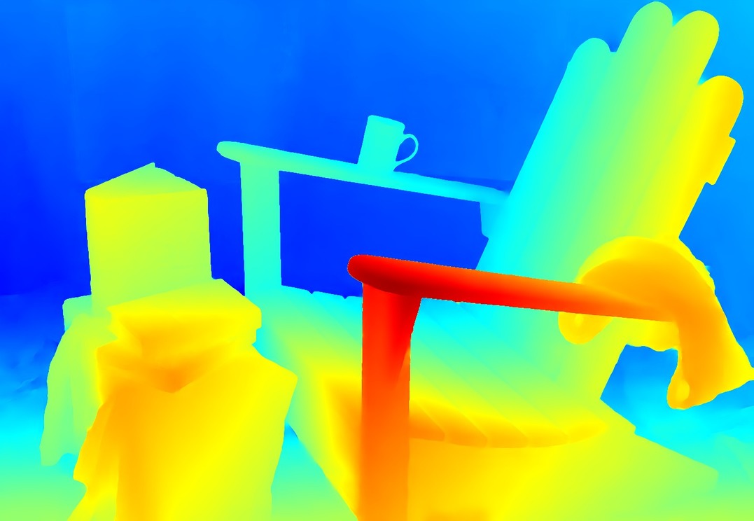
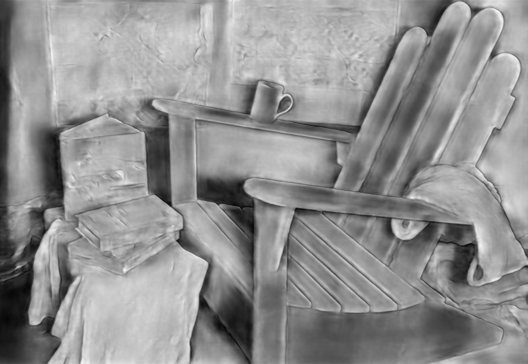
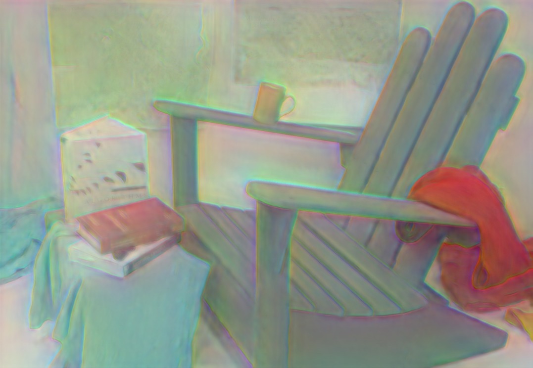
Learned Collaborative Stereo Refinement
Abstract
In this work, we propose a learning-based method to denoise and refine disparity maps of a given stereo method. The proposed variational network arises naturally from unrolling the iterates of a proximal gradient method applied to a variational energy defined in a joint disparity, color, and confidence image space. Our method allows to learn a robust collaborative regularizer leveraging the joint statistics of the color image, the confidence map and the disparity map. Due to the variational structure of our method, the individual steps can be easily visualized, thus enabling interpretability of the method. We can therefore provide interesting insights into how our method refines and denoises disparity maps. The efficiency of our method is demonstrated by the publicly available stereo benchmarks Middlebury 2014 and Kitti 2015.
1 Introduction
Computing 3D information from a stereo pair is one of the most important problems in computer vision. One reason for this is that depth information is a very strong cue to understanding visual scenes, and depth information is therefore an integral part of many vision based systems. For example, in autonomous driving, it is not sufficient to know the objects visible in the scene, but it is also important to estimate the distance to these objects. A lidar scanner is often too expensive and provides only sparse depth estimates. Therefore, it is an interesting alternative to compute depth information exclusively from stereo images. However, the calculation of depth information from images is still a very challenging task. Reflections, occlusions, challenging illuminations etc. make the task even harder. To tackle these difficulties the computation of dense depth maps is usually split up into the four steps (i) matching cost computation, (ii) cost aggregation, (iii) disparity computation and (iv) disparity refinement [27]. In deep learning based approaches (i) and (ii) are usually implemented in a matching convolutional neural network (CNN), (iii) is done using graphical models or 3D regularization CNNs and (iv) is done with a refinement module [29].
There are many approaches to tackle (i)-(iii). However, there are only a few learning-based works for disparity refinement (iv) (see Section 2). Existing work to refine the disparity map is often based on another CNN using residual connections. In this work we want to overcome these black-box refinement networks with a simple, effective and most important easily interpretable refinement approach for disparity maps. We tackle the refinement problem with a learnable hierarchical variational network. This allows us to exploit both the power of deep learning and the interpretability of variational methods. In order to show the effectiveness of the proposed refinement module, we conduct experiments on directly refining/denoising winner-takes-all (WTA) solutions of feature matching and as a pure post-processing module on top of an existing stereo method. Fig. 1 shows an overview of our method. Starting from an initial disparity map the final result is iteratively reconstructed.
Contributions
We propose a learnable variational refinement network which takes advantage of the joint information of the color image, the disparity map and a confidence map to compute a regularized disparity map. We therefore show how our proposed method can be derived from the iterates of a proximal gradient method and how it can be specifically designed for stereo refinement. Additionally, we evaluate a broad range of possible architectural choices in an ablation study. Furthermore, we give insights into how our model constructs the final disparity map by visualizing and interpreting the intermediate iterates. We show the effectiveness of our method by participating on the two complementary public available benchmarks Middlebury 2014 and Kitti 2015.
2 Related Work
We propose a learnable variational model, where we use the modeling power of variational calculus to explicitly guide the refinement process for stereo. Thus, we focus on disparity refinement in the following sections.
Variational Methods
Variational methods formulate the correspondence problem as minimization of an energy functional comprising a data fidelity term and a smoothness term. We also briefly review variational optical flow methods, because stereo is a special case of optical flow, i.e. it can be considered as optical flow in horizontal direction only. The data-term measures usually the raw intensity difference [3, 32, 4] between the reference view and the warped other view. The regularizer imposes prior knowledge on the resulting disparity map. This is, the disparity map is assumed to be piecewise smooth. Prominent regularizers are the robust Total Variation (TV) [32] and the higher order generalization of TV as e.g. used by Ranftl et al. [20, 21] or by Kuschk and Cremers [13]. Variational approaches have two important advantages in the context of stereo. They naturally produce sub-pixel accurate disparities and they are easily interpretable. However, in order to also capture large displacements a coarse-to-fine warping scheme [3] is necessary. To overcome the warping scheme without losing fine details, variational methods can also be used to refine an initial disparity map. This has e.g. be done by Shekhovtsov et al. [28] who refined the initial disparity estimates coming from a Conditional Random Field (CRF). Similarly, [22] and [16] used a variational method for refining optical flow.
Disparity Refinement
Here we want to focus on the refinement of an initial disparity map. The initial disparity map can be e.g. the WTA solution of a matching volume or any other output of a stereo algorithm. One important approach of refinement algorithms is the fast bilateral solver (FBS) [1]. This algorithm refines the initial disparity estimate by solving an optimization problem containing an smoothness- and an data-fidelity term. The fast bilateral solver is the most related work to ours. However, in this work we replace the norm with the robust norm. More importantly, we additionally replace the hand-crafted smoothness term by a learnable multi-scale regularizer. Another refinement method was proposed by Gidaris and Komodakis [7]. They also start with an initial disparity map, detect erroneous regions and then replace and refine these regions to get a high-quality output. Pang et al. [18] proposed to apply one and the same network twice. They compute the initial disparity map in a first pass, warp the second view with the initial disparity map and then compute only the residual to obtain a high quality disparity map. Liang et al. [14] also improved the results by adding a refinement sub-network on top of the regularization network. We want to stress that the CNN based refinement networks [14, 18] do not have a specialized architecture for refinement as opposed to the proposed model.
Learnable optimization schemes
Learnable optimization schemes are based on unrolling the iterates of optimization algorithms. We divide the approaches into two categories. In the first category the optimization iterates are mainly used to utilize the structure during learning. For example in [23] 10 iterations of a TGV regularized variational method are unrolled and used for depth super-resolution. However, they kept the algorithm fixed, i.e. the only learnable parameters in the inference part are the step-sizes. Similarly, in [30] unrolling 10k iterations of the FISTA [2] algorithm is proposed. The second category includes methods where the optimization scheme is not only used to provide the structure, but it is also generalized by adding additional learnable parameters directly to the optimization iterates. For example [31] proposed a primal-dual-network for low-level vision problems, where the authors learned the inference part of a Markov Random Field (MRF) model generalizing a primal-dual algorithm. Chen et al. [6] generalized a reaction-diffusion model and successfully learned a model for image denoising. Based on [6] a generalized incremental proximal gradient method was proposed in [12], where the authors showed connections to residual units [8]. We built on the work of Chen et al., but specially designed the energy terms for the stereo task. Additionally, we allow to regularize on multiple spatial resolutions jointly and make use of the robust function in our data-terms.
3 Method
We consider images to be functions , with and is the number of channels which is 3 for RGB color images. Given two images and from a rectified stereo pair, we want to compute dense disparities such that , i.e. we want to compute the horizontal shift for each pixel between the reference image and the second image . Here, we propose a novel variational refinement network for stereo which operates solely in 2D image space and is thus very efficient. The input to our method is an initial disparity map , where is the maximal disparity, a reference image and a pixel-wise confidence map . The proposed variational network is a method to regularize, denoise and refine a noisy disparity map with learnable filters and learnable potential functions. Hence, the task we want to solve is the following: Given a noisy disparity map , we want to recover the clean disparity with learnable variational network steps. We do not make any assumptions on the quality of the initial disparity map, i.e. the initial disparity map may contain many strong outliers.
3.1 Collaborative Disparity Denoising
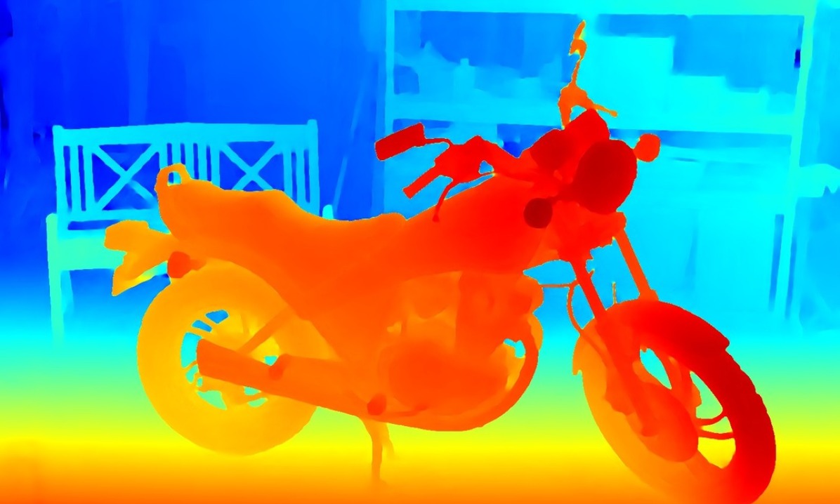
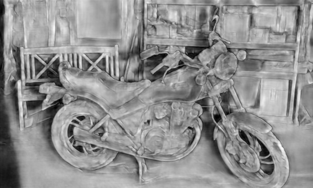
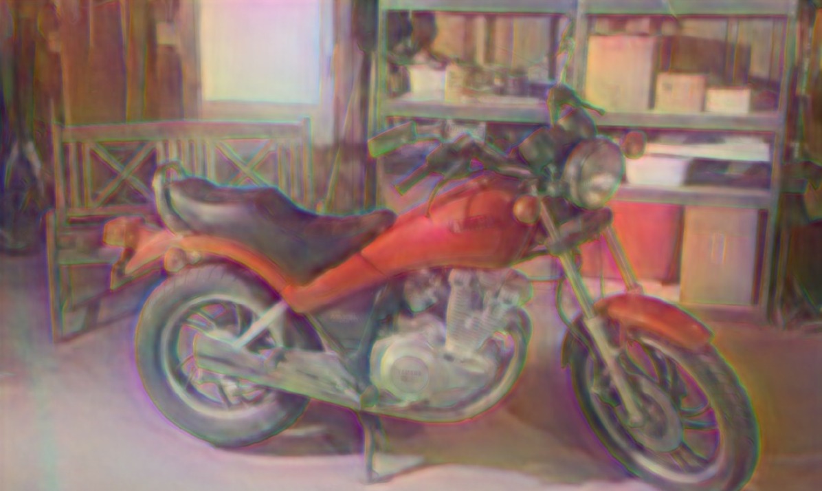
As the main contribution of this paper, we propose a method that performs a collaborative denoising in the joint color image, disparity and confidence space (see Fig. 2). Our model is based on the following three observations: (i) Depth discontinuities co-inside with object boundaries, (ii) discontinuities in the confidence image are expected to be close to left-sided object boundaries and (iii) the confidence image can be used as a pixel-wise weighting factor in the data fidelity term. Based on these three observations, we propose the following collaborative variational denoising model
| (1) |
where , i.e. contains for every pixel an RGB color information, a disparity value and a confidence value. denotes the collaborative regularizer and it is given by a multi-scale and multi-channel version of the Fields of Experts (FoE) model [25] with scales and channels.
| (2) |
where are combined blur and downsampling operators, are linear convolution operators and are non-linear activation functions. The vector holds the parameters of the regularizer which will be detailed later. Note that multiple levels allow the model to operate on different spatial resolutions and therefore enables the denoising of large corrupted areas. Intuitively, the collaborative regularizer captures the statistics of the joint color, confidence and disparity space. Hence, it will be necessary to learn the linear operators and the non-linear potential functions from data. It will turn out that the combination of filtering in the joint color-disparity-confidence space at multiple hierarchical pyramid levels and specifically learned channel-wise potential functions make our model very powerful.
denotes the collaborative data fidelity term and it is defined by
| (3) |
where is again a placeholder for the learnable parameters. The first term ensures that the smoothed color image does not deviate too much from the original color image , the second term ensures that the smoothed confidence map stays close to the original confidence map. Here we use an norm in order to deal with outliers in the initial confidence map. The last term is the data fidelity term of the disparity map. It is given by an norm which is pixel-wise weighted by the confidence measure . Hence, data fidelity is enforced in high-confidence regions and suppressed in low-confidence regions. Note that the weighted norm additionally ties the disparity map with the confidence map during the steps of the variational network.
Proximal Gradient Method (PGM)
We consider a PGM [19] whose iterates are given by
| (4) |
where is the step-size, is the gradient of the regularizer which is given by
| (5) |
where . denotes the proximal operator with respect to the data fidelity term, which is defined by
| (6) |
Note that the proximal map allows to handle the non-smooth data fidelity terms such as the norm. Additionally, there is a strong link between proximal gradient methods and residual units which allows to incrementally reconstruct a solution (see Fig. 1). We provide the computation of the prox-terms in the supplementary material.
Variational Network
Our collaborative denoising algorithm consists of performing a fixed number of iterations of the proximal gradient method Eq. 4. In order to increase the flexibility we allow the model parameters to change in each iteration.
| (7) |
Following [6, 12] we parametrize the derivatives of the potential functions using Gaussian radial basis functions (RBF)
| (8) |
where are the means regularly sampled on the interval , is the standard deviation of the Gaussian kernel and is a scaling factor. The linear operators are implemented as multi-channel 2D convolutions with convolution kernels . In summary, the parameters in each step are given by .
4 Computing Inputs
Our proposed refinement method can be applied to an arbitrary stereo method, provided it comes along with a cost-volume, which is the case for the majority of existing stereo methods.
Probability volume
Assume we have given a cost-volume , where smaller costs mean a higher likelihood of the respective disparity values. In order to map the values onto probabilities , we make use of the “softmax” function, that is
| (9) |
where influences the smoothness of the probability distribution.
Initial disparity map
From Eq. 9 we can compute the WTA solution by a pixel-wise arg max over the disparity dimension, i.e.,
| (10) |
Moreover, we compute a sub-pixel accurate disparity map by fitting a quadratic function to the probability volume. This is equivalent to perform one step of Newton’s algorithm:
| (11) |
where denote standard forward and backward differences in the disparity dimension. Furthermore, we compute the refined value of the probabilities, denoted as , via linear interpolation in the probability volume.
Initial Confidence Measure
The computation of a confidence measure of the stereo results is important for many applications and a research topic on its own [9]. Here we take advantage of the probabilistic nature of our matching costs . Moreover, we make use of geometric constraints by using a left-right (LR) consistency check, where the left and right images are interchanged. This allows us to identify occluded regions. We compute the probability of a pixel being not occluded as
| (12) |
where
| (13) |
is the disparity difference between the left prediction and the right prediction and the parameter acts as a threshold and is set to in all experiments. The final confidence measure is given by
| (14) |
Thus, we define our total confidence as the product of the matching confidence and the LR confidence. Most of the pixels not surviving the LR check are pixels in occluded regions. To get a good initialization for these pixels as well, we inpaint the disparities of these pixels from the left side. The experiments show that this significantly increases the performance of the model (see Table 1).
5 Learning
In this section we describe our learning procedure for the collaborative denoising model. To remove scaling ambiguities we require the filter kernels to be zero-mean and to have an norm . Moreover, we constraint the weights of the RBF kernels to have an norm , too. This is defined with the following convex set:
| (15) |
For learning, we define a loss function that measures the error between the last iterate of the disparity map and the ground-truth disparity . Note that we do not have a loss function for the confidence and the color image. Their aim is rather to support the disparity map to achieve the lowest loss. We use a truncated Huber function of the form
| (16) |
where is a truncation value, denotes the index of the training sample and
| (17) |
is the Huber function.
| Init | Step 1 | Step 2 | Step 3 | Step 4 | Step 5 | Step 6 | Step 7 |
Implementation details
We implemented our model in the PyTorch machine learning framework111https://pytorch.org. We train the refinement module for 3000 epochs with a learning rate of with a modified projected Adam optimizer [10]. We dynamically adjusted the stepsize computation to be constant within each parameter block in our constraint set to ensure that we perform an orthogonal projection onto the constraint set. After 1500 epochs we reduce the truncation value from to .
6 Experiments
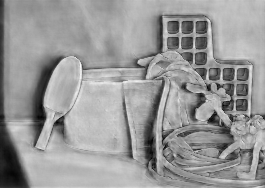
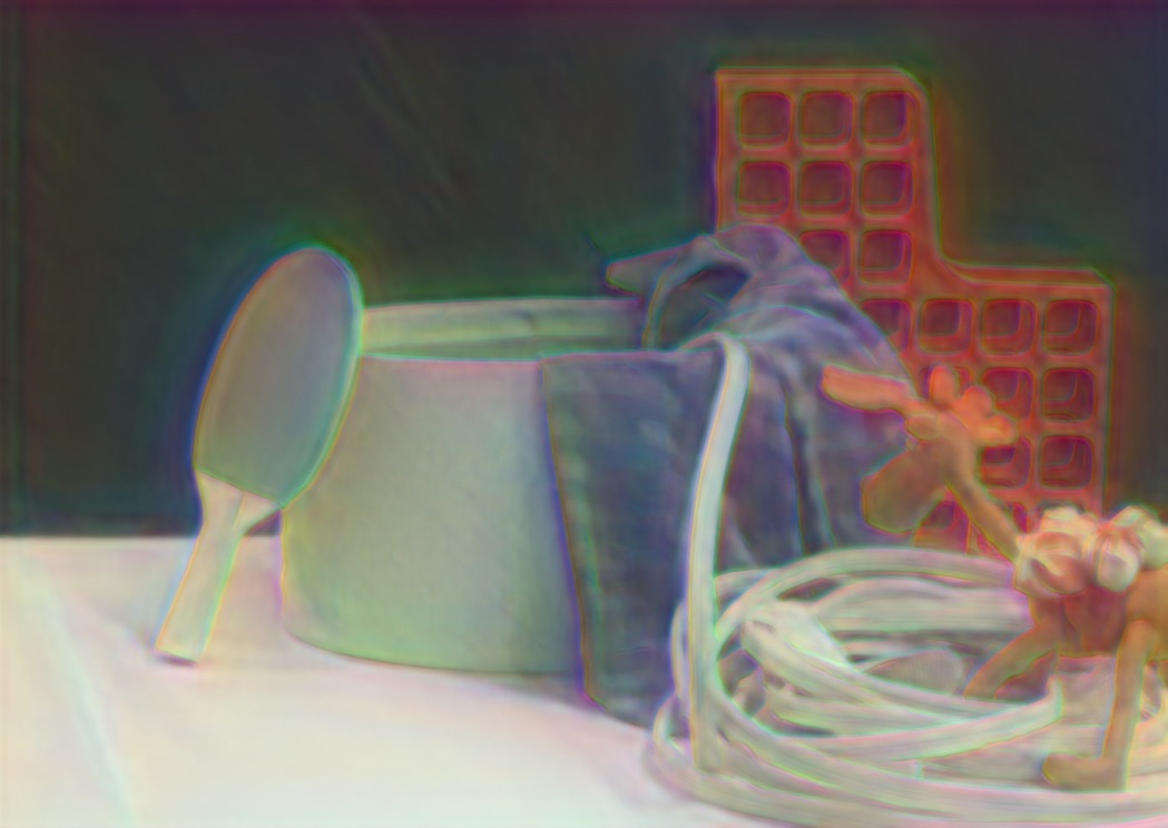
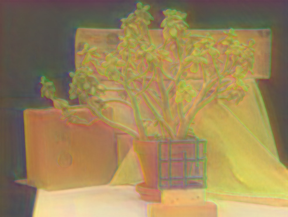
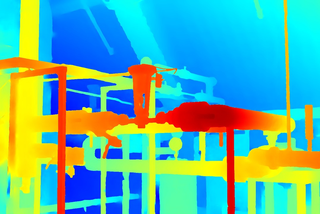
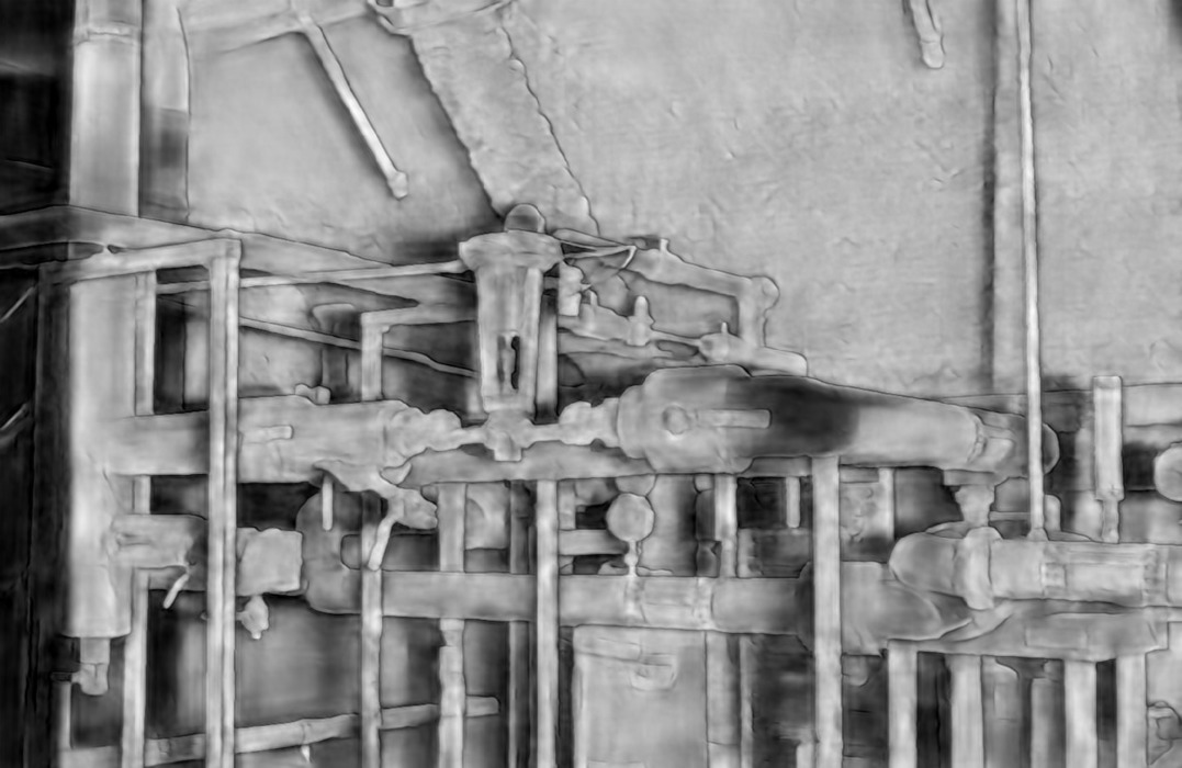
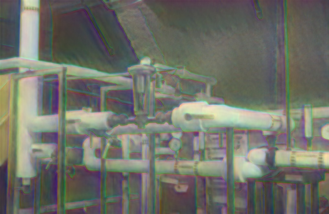
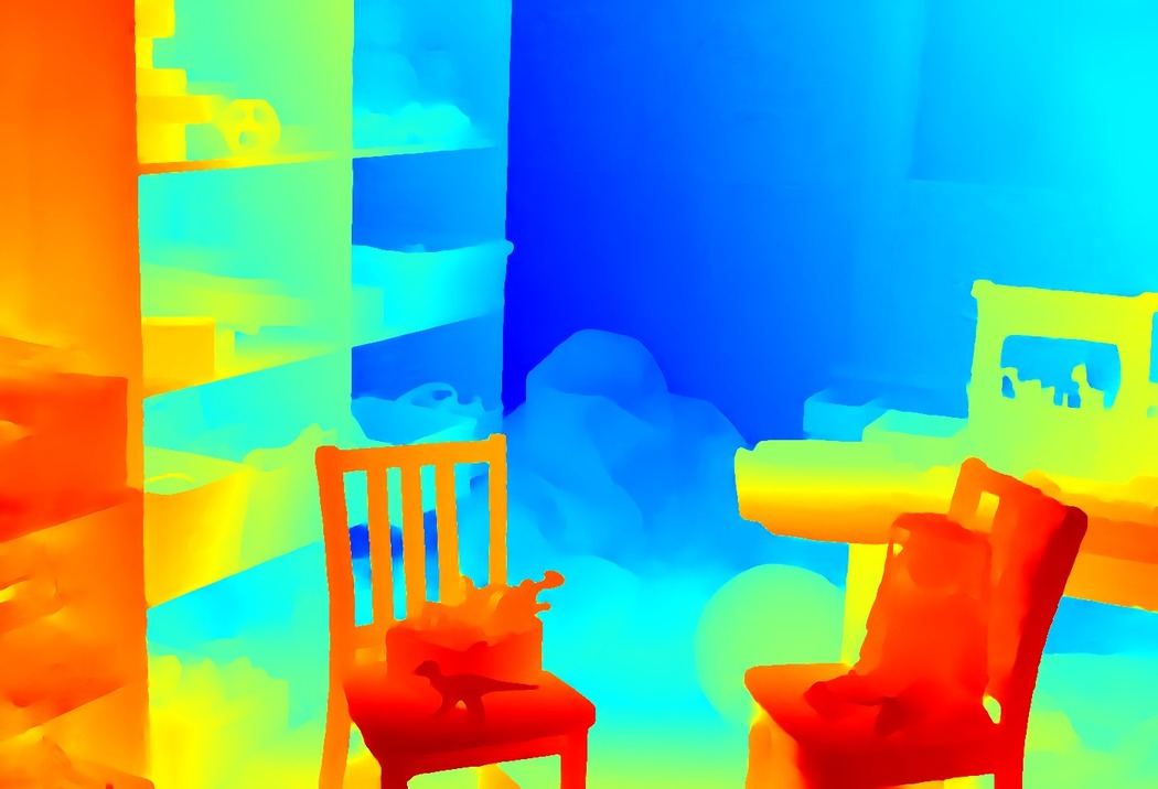
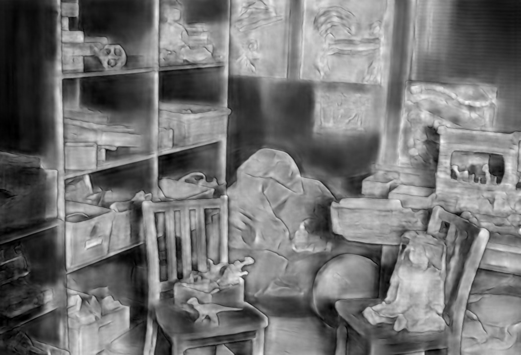
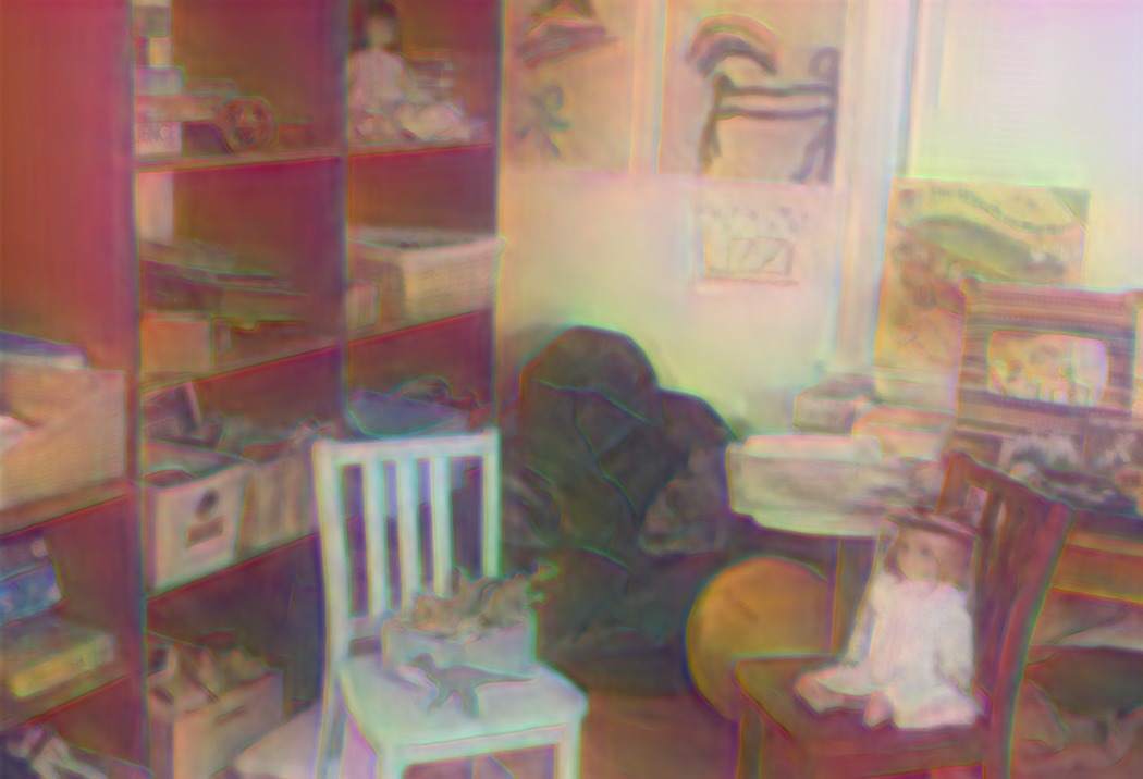
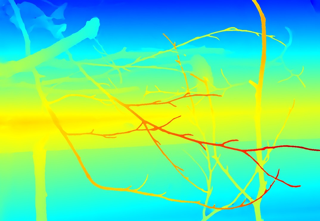
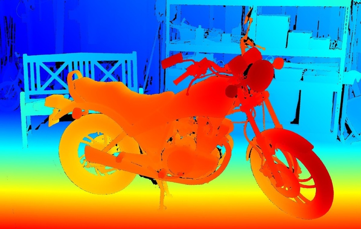
We split the experiments into two parts. In the first part we evaluate architectural choices based on the WTA result of a matching network and compare with the FBS [1]. In the second part, we use the best architecture and train a variational network for refining the disparity maps computed by the CNN-CRF method [11]. We use this method to participate in the public available stereo benchmarks Middlebury 2014 and Kitti 2015. To ensure a fair comparison we choose methods with similar numbers of parameters and runtimes. Fig. 3 shows how our method constructs the final result. The method recovers step-by-step fine details with the guidance of the confidences and the color image.


Kitti 2015
The Kitti 2015 dataset [17] is an outdoor dataset specifically designed for autonomous driving. It contains 200 images with available ground-truth to train a model and 200 images with withheld ground-truth which is used for testing the models on previously unseen data. The ground-truth is captured using a laser scanner and is therefore sparse in general. The cars are densified by fitting CAD models into the laser point-cloud. We report the badX error metric for occluded (occ) and non-occluded (noc) pixels with . In the badX measure the predicted disparity is treated incorrect, if the distance to the ground-truth disparity is larger than .
Middlebury 2014
The Middlebury 2014 stereo dataset [26] is orthogonal to the Kitti 2015 dataset. It consists of 153 high resolution indoor images with highly precise dense ground-truth. The challenges in the Middlebury dataset are large, almost untextured regions, huge occluded regions, reflections and difficult lighting conditions. The generalization capability of the method is evaluated on a 15 images test-set with withheld ground-truth data. We report all available metrics, i.e., bad errors, the average error (avg) and the root-mean-squared error (rms).
6.1 Ablation Study
| Model | WTA | FBF [1] | VN | VN | VN | VN | VN | VN | VN | VN | VN | VN | |
| Conf | ✓ | ✓ | ✓ | ✓ | ✓ | ✓ | ✓ | ✓ | ✓ | ||||
| Img | ✓ | ✓ | ✓ | ✓ | ✓ | ✓ | ✓ | ✓ | ✓ | ||||
| OccIp | ✓ | ✓ | ✓ | ✓ | ✓ | ✓ | ✓ | ✓ | ✓ | ✓ | |||
| Joint | ✓ | ✓ | ✓ | ✓ | ✓ | ||||||||
| [bad3] | occ | 8.24 | 7.48 | 5.42 | 5.12 | 4.43 | 3.77 | 3.46 | 3.37 | 3.43 | 3.62 | 4.37 | 4.25 |
| noc | 6.78 | 6.08 | 4.68 | 3.98 | 3.90 | 3.07 | 2.72 | 2.55 | 2.58 | 2.97 | 3.71 | 3.49 | |
To find the most appropriate hyper parameters for the proposed method, we generate our initial disparity map with a simple feature network. The learned features are then compared using a fixed matching function for a pre-defined number of discrete disparities.
Feature Network
Our feature network is a modified version of the U-Net [24, 15] which we use to extract features suitable for stereo matching. We kept the number of parameters low by only using 64 channels at every layer. The output of our feature network is thus a 64-dimensional feature vector for every pixel. The exact architecture is shown in the supplementary material.
Feature Matching
Next, we use the extracted features from the left image and from the right image to compute a matching score volume with
| (18) |
We follow Section 4 to compute the inputs for the variational network.
Ablation Study
We systematically remove parts of our method in order to show how the final performance is influenced by the individual parts. Table 1 shows an overview of all experiments. First we investigate the influence of our data-terms, the disparity data-term, the confidence data-term and the RGB image data-term. The study shows that each of the data-terms positively influence the final performance. Especially, adding the original input image significantly increases the performance. This can be e.g. seen in Fig. 3, where the information of how the basket needs to be reconstructed, is derived from the input image. In the second part of the study, we evaluate different variational network architectures. To make the comparison as fair as possible, we chose the variants such that the total number of parameters is approximately the same for all architectures. The experiments show, that a compromise between number of steps, pyramid levels and filter-size yields the best results. The best performing model is the model , where the filter-size is set to for pyramid levels and steps. The average runtime of this VN is as low as 0.09s on an NVidia 2080Ti graphics card.
Additionally, we compare with the FBS. We therefore use exactly the same inputs as we did in our method, i.e., the refined WTA solution , our confidence measure and the RGB input image. To ensure the best performance for the FBS, we performed a grid-search over its hyper-parameters on the Kitti dataset. As shown in Table 1 the FBS clearly improves the performance upon the initial solution, but the FBS cannot compete with the proposed method.
6.2 Benchmark Performance
We use our method on top of the CNN-CRF [11] stereo method for the official test set evaluation (see Table 2). We set the temperature parameter in all experiments. The average rank is computed with all published methods in the respective benchmarks with a runtime . This yields in total 71 methods on the Kitti benchmark and 50 methods on the Middlebury benchmark.
| Method | Kitti 2015 | Middlebury 2014 | |||||||||
| noc | all | R | bad0.5 | bad1 | bad2 | bad4 | avg | rms | time | R | |
| PSMNet [5] | - | 1.83 | - | 90.0 | 78.1 | 58.5 | 32.2 | 9.60 | 21.7 | 2.62 | 44 |
| PDS [29] | - | - | - | 54.2 | 26.1 | 11.4 | 5.10 | 1.98 | 9.10 | 10 | 8 |
| MC-CNN [33] | - | - | - | 42.1 | 20.5 | 11.7 | 7.94 | 3.87 | 16.5 | 1.26 | 9 |
| CNN-CRF [11] | - | 4.04 | - | 56.1 | 25.1 | 10.8 | 6.12 | 2.30 | 9.89 | 3.53 | 10 |
| [11] + VN (ours) | 1.90 | 2.04 | - | 41.8 | 17.1 | 7.05 | 2.96 | 1.21 | 5.80 | 4.06 | 2 |
| PSMNet [5] | 2.14 | 2.32 | 17 | 81.1 | 63.9 | 42.1 | 23.5 | 6.68 | 19.4 | 2.62 | 33 |
| PDS [29] | 2.36 | 2.58 | 19 | 58.9 | 21.1 | 14.2 | 6.98 | 3.27 | 15.7 | 10.3 | 9 |
| MC-CNN [33] | 3.33 | 3.89 | 32 | 41.3 | 18.0 | 9.47 | 6.7 | 4.37 | 22.4 | 1.26 | 6 |
| CNN-CRF [11] | 4.84 | 5.50 | 36 | 60.9 | 31.9 | 12.5 | 6.61 | 3.02 | 14.4 | 3.53 | 8 |
| [11] + VN (ours) | 4.45 | 4.85 | 33 | 56.2 | 30.0 | 14.2 | 7.71 | 2.49 | 10.8 | 4.06 | 6 |
| Initial |
|
|
| Refined |
|
|
We used the model VN on the Kitti dataset. As shown in Table 2 we reduce the bad3 error in both, occluded and in non-occluded regions. Fig. 4 shows qualitative results with the corresponding error maps on the Kitti test set.
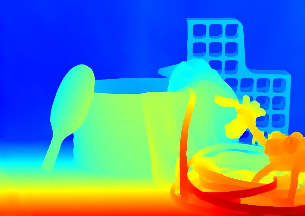
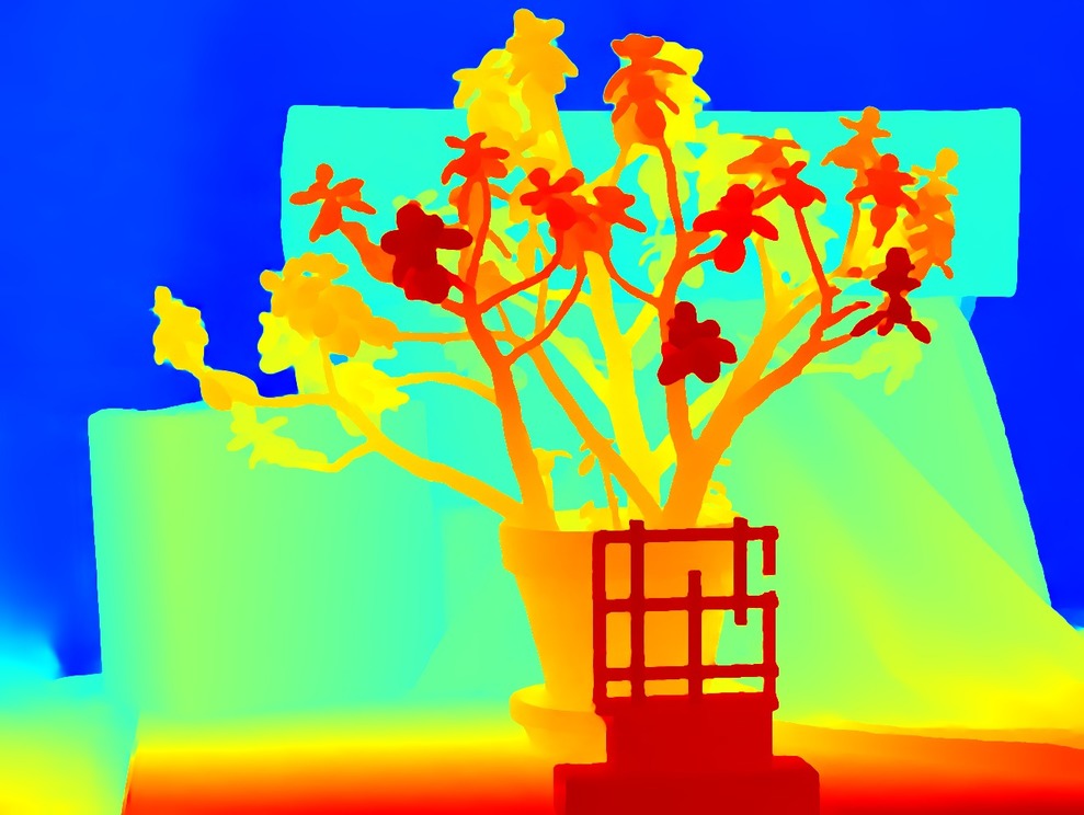
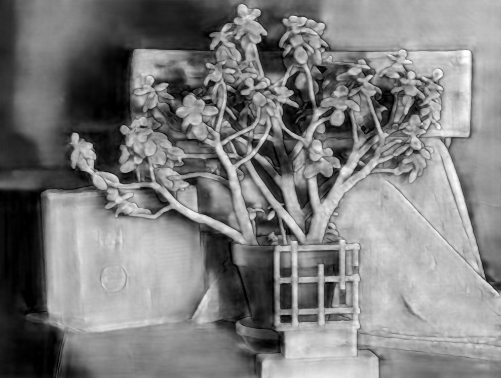
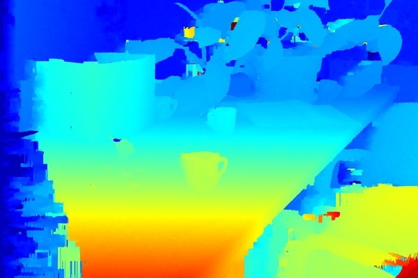
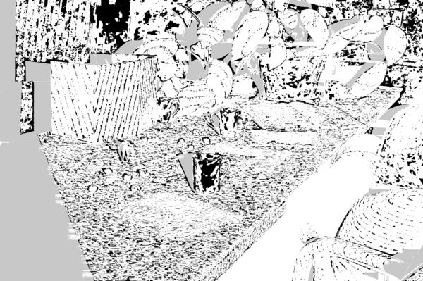
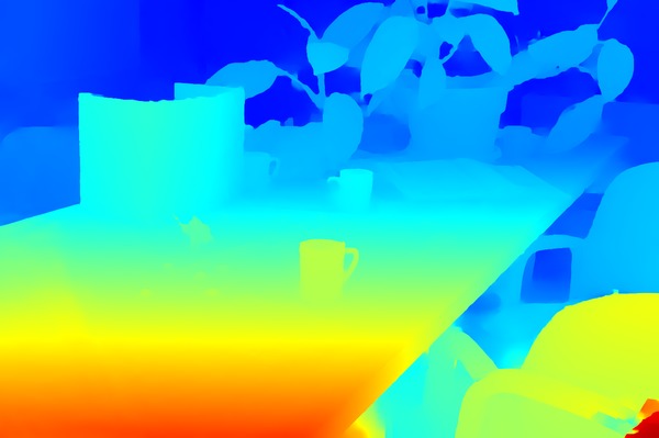
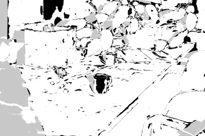
On the Middlebury benchmark we use the model VN for all evaluations. We compare the errors on the training set with the errors on the test set (Table 2) and observe that: (i) Our method achieves the best scores in all metrics among the compared methods on the training set. (ii) This positive trend is transferred to the test set for the average error and the RMS error. (iii) The bad errors on the test set are reduced and (iv) the bad errors slightly increase on the test set compared to [11]. One reason for this is the limited amount of training data for these very high-resolution images. Fig. 5 shows a qualitative example of the Middlebury test set. Note that the tabletop is nice and smooth while the sharp edges of the objects are very well preserved.
7 Conclusion & Future Work
We have proposed a learnable variational network for efficient refinement of disparity maps. The learned collaborative and hierarchical refinement method allows the use of information from the joint color, confidence and disparity space from multiple spatial resolutions. In an ablation study, we evaluated a broad range of architectural choices and demonstrated the impact of our design decisions. Our method can be applied on top of any other stereo method, with full use of additional information of a full cost volume. We demonstrated this by adding the variational refinement network on top of the CNN-CRF method and have shown improved results. Furthermore, we have proven the effectiveness of our method by participating in the publicly available stereo benchmarks of Middlebury and Kitti. In future work, we would like to include a matching score during the refinement process and perform data augmentation to increase the training set for learning.
Acknowledgements. This work was partly supported from the ERC starting grant HOMOVIS (No.640156).
References
- [1] Barron, J.T., Poole, B.: The fast bilateral solver. In: European Conference on Computer Vision (ECCV). pp. 617–632 (2016)
- [2] Beck, A., Teboulle, M.: A fast iterative shrinkage-thresholding algorithm for linear inverse problems. SIAM J. Imaging Sciences pp. 183–202 (2009)
- [3] Brox, T., Bruhn, A., Papenberg, N., Weickert, J.: High accuracy optical flow estimation based on a theory for warping. In: European Conference on Computer Vision (ECCV). pp. 25–36 (2004)
- [4] Chambolle, A., Pock, T.: A first-order primal-dual algorithm for convex problems with applications to imaging. Journal of Mathematical Imaging and Vision pp. 120–145 (2011)
- [5] Chang, J.R., Chen, Y.S.: Pyramid stereo matching network. In: IEEE Conference on Computer Vision and Pattern Recognition (CVPR). pp. 5410–5418 (2018)
- [6] Chen, Y., Yu, W., Pock, T.: On learning optimized reaction diffusion processes for effective image restoration. In: IEEE Conference on Computer Vision and Pattern Recognition (CVPR). pp. 5261–5269 (2015)
- [7] Gidaris, S., Komodakis, N.: Detect, replace, refine: Deep structured prediction for pixel wise labeling. In: IEEE Conference on Computer Vision and Pattern Recognition (CVPR). pp. 5248–5257 (2017)
- [8] He, K., Zhang, X., Ren, S., Sun, J.: Deep residual learning for image recognition. In: IEEE Conference on Computer Vision and Pattern Recognition (CVPR). pp. 770–778 (June 2016)
- [9] Hu, X., Mordohai, P.: A quantitative evaluation of confidence measures for stereo vision. IEEE Transactions on Pattern Analysis and Machine Intelligence pp. 2121–2133 (2012)
- [10] Kingma, D.P., Ba, J.: Adam: A method for stochastic optimization. arXiv preprint arXiv:1412.6980 (2014)
- [11] Knöbelreiter, P., Reinbacher, C., Shekhovtsov, A., Pock, T.: End-to-end training of hybrid cnn-crf models for stereo. In: IEEE Conference on Computer Vision and Pattern Recognition (CVPR). pp. 2339–2348 (2017)
- [12] Kobler, E., Klatzer, T., Hammernik, K., Pock, T.: Variational networks: Connecting variational methods and deep learning. In: German Conference on Pattern Recognition (GCPR). pp. 281–293 (2017)
- [13] Kuschk, G., Cremers, D.: Fast and accurate large-scale stereo reconstruction using variational methods. In: IEEE International Conference on Computer Vision Workshop. pp. 700–707 (2013)
- [14] Liang, Z., Feng, Y., Guo, Y., Liu, H., Chen, W., Qiao, L., Zhou, L., Zhang, J.: Learning for disparity estimation through feature constancy. In: IEEE Conference on Computer Vision and Pattern Recognition (CVPR). pp. 2811–2820 (2018)
- [15] Long, J., Shelhamer, E., Darrell, T.: Fully convolutional networks for semantic segmentation. In: IEEE Conference on Computer Vision and Pattern Recognition (CVPR). pp. 3431–3440 (2015)
- [16] Maurer, D., Stoll, M., Bruhn, A.: Order-adaptive and illumination-aware variational optical flow refinement. In: British Machine Vision Conference (2017)
- [17] Menze, M., Geiger, A.: Object scene flow for autonomous vehicles. In: IEEE Conference on Computer Vision and Pattern Recognition (CVPR). pp. 3061–3070 (2015)
- [18] Pang, J., Sun, W., Ren, J.S., Yang, C., Yan, Q.: Cascade residual learning: A two-stage convolutional neural network for stereo matching. In: IEEE International Conference on Computer Vision Workshop. pp. 887–895 (2017)
- [19] Parikh, N., Boyd, S., et al.: Proximal algorithms. Foundations and Trends® in Optimization pp. 127–239 (2014)
- [20] Ranftl, R., Gehrig, S., Pock, T., Bischof, H.: Pushing the limits of stereo using variational stereo estimation. In: IEEE Intelligent Vehicles Symposium. pp. 401–407 (2012)
- [21] Ranftl, R., Bredies, K., Pock, T.: Non-local total generalized variation for optical flow estimation. In: European Conference on Computer Vision (ECCV). pp. 439–454 (2014)
- [22] Revaud, J., Weinzaepfel, P., Harchaoui, Z., Schmid, C.: Epicflow: Edge-preserving interpolation of correspondences for optical flow. In: IEEE Conference on Computer Vision and Pattern Recognition (CVPR). pp. 1164–1172 (2015)
- [23] Riegler, G., Rüther, M., Bischof, H.: Atgv-net: Accurate depth super-resolution. In: European Conference on Computer Vision (ECCV). pp. 268–284 (2016)
- [24] Ronneberger, O., Fischer, P., Brox, T.: U-net: Convolutional networks for biomedical image segmentation. In: International Conference on Medical Image Computing and Computer-Assisted Intervention (MICCAI). pp. 234–241 (2015)
- [25] Roth, S., Black, M.J.: Fields of experts. International Journal of Computer Vision (2009)
- [26] Scharstein, D., Hirschmüller, H., Kitajima, Y., Krathwohl, G., Nesic, N., Wang, X., Westling, P.: High-resolution stereo datasets with subpixel-accurate ground truth. In: German Conference on Pattern Recognition (GCPR). pp. 31–42 (2014)
- [27] Scharstein, D., Szeliski, R.: A taxonomy and evaluation of dense two-frame stereo correspondence algorithms. International Journal of Computer Vision (2002)
- [28] Shekhovtsov, A., Reinbacher, C., Graber, G., Pock, T.: Solving dense image matching in real-time using discrete-continuous optimization. Computer Vision Winter Workshop (2016)
- [29] Tulyakov, S., Ivanov, A., Fleuret, F.: Practical deep stereo (pds): Toward applications-friendly deep stereo matching. In: Proceedings of Advances in Neural Information Processing Systems. pp. 5871–5881 (2018)
- [30] Vogel, C., Knöbelreiter, P., Pock, T.: Learning energy based inpainting for optical flow. In: Asian Conference on Computer Vision (ACCV) (2018)
- [31] Vogel, C., Pock, T.: A primal dual network for low-level vision problems. In: German Conference on Pattern Recognition (GCPR) (2017)
- [32] Zach, C., Pock, T., Bischof, H.: A duality based approach for realtime tv-l1 optical flow. In: German Conference on Pattern Recognition (GCPR) (2007)
- [33] Žbontar, J., LeCun, Y.: Stereo matching by training a convolutional neural network to compare image patches. Journal of Machine Learning Research (2016)
Learned Collaborative Stereo Refinement
Supplementary Material
1 Proximal Operators for the data terms
We provide the solution of the proximal operators used in the data terms. The proximal operator is defined as the optimization problem
| (19) |
In the main paper we used the proximal operator with and functions. The prox is used for the color image and the prox for the confidences and the disparities. We will present the closed form solutions for these two cases in the next paragraphs.
Proximal operator for functions
Proximal operator for functions
Similarly, we compute the proximal operator of the following weighted function
| (22) |
The absolute function is not differentiable at 0 and therefore the optimality condition requires the sub-differential to contain 0. The closed form solution of the proximal operator Eq. 19 with being the function as defined in Eq. 22 is given by
| (23) |
Thus, for the confidence data term and and for the disparity data term and .
2 Derivative of the quadratic fitting
In the joint training of our feature network and the regularization network we need to backpropagate the gradient through the refined disparities. Therefore, we must compute the gradient of our sub-pixel accurate disparity map w.r.t. the probability volume. The gradient is non-zero only for the supporting points of the quadratic function (shown in blue in Fig. 1). Precisely, it is given by
| (24) |
where are standard forward-, backward- and central-differences in the disparity dimension. Note, that we overcome the problem of the non-differentiable function with the fitting of the quadratic function.
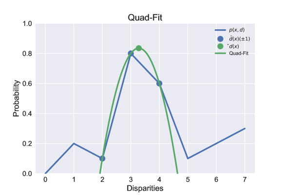
Fig. 1 shows a visualization of the quadratic fitting procedure.
3 Architecture of the feature network
The detailed architecture of our feature network is shown in Table 1. It is a variant of a U-Net with two spatial resolutions and 64 channels in every layer. In the contraction part the resolution is reduced every 2 layers. In the expansion part features are upsampled with transposed convolutions and concatenated with the extracted features of the same resolution to keep fine details.
| Layer | KS | Resolution | Channels | Input |
| conv00 | 3 | Image | ||
| conv01 | 3 | conv00 | ||
| pool0 | 2 | conv01 | ||
| conv10 | 3 | pool0 | ||
| conv11 | 3 | conv10 | ||
| pool1 | 2 | conv10 | ||
| conv20 | 3 | pool1 | ||
| conv21 | 3 | conv20 | ||
| deconv1 | 3 | conv21 | ||
| conv12 | 3 | {deconv1, conv11} | ||
| conv13 | 3 | conv12 | ||
| deconv0 | 3 | conv12 | ||
| conv02 | 3 | {deconv0, conv01} | ||
| conv03 | 3 | conv02 |
4 Learned filters and activation functions
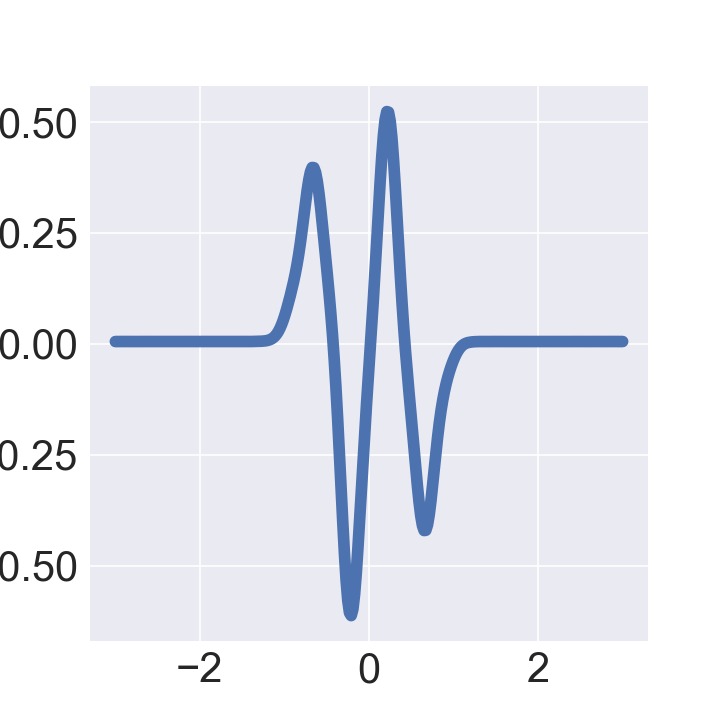
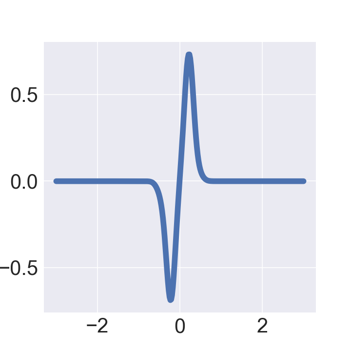
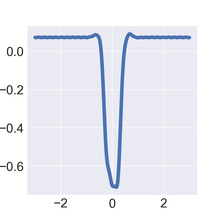
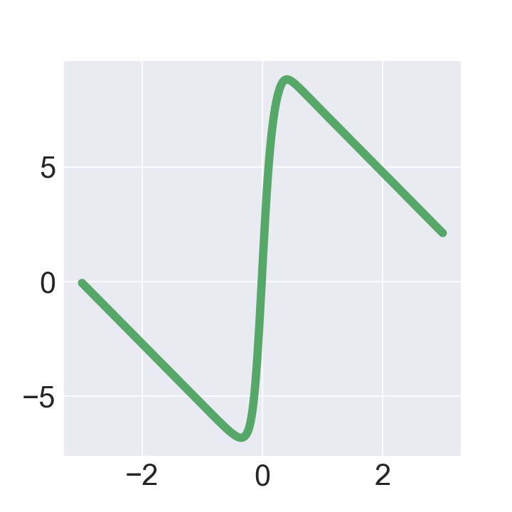
We give further insights into what and how our model learns by visualizing the filters and activation functions learned by our model. Fig. 2(a) shows selected filter kernels. The first row contains filters for the disparity map, the second row contains filters for the RGB color image and the third row contains filters for the confidence map. Note that the learned filters are interpretable because they contain structure. This suggests that our model captures statistics of how to appropriately denoise disparity maps, confidence maps and color images jointly.
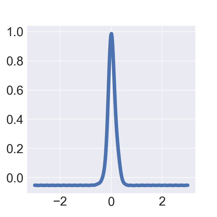
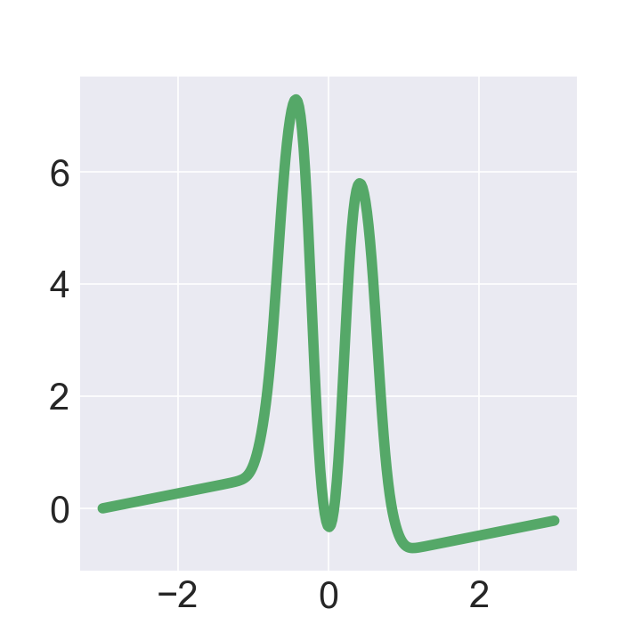
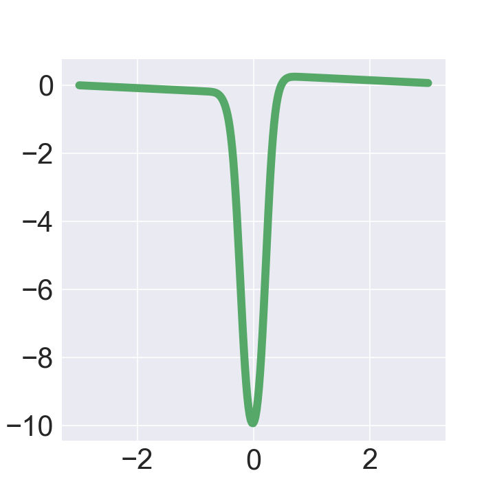
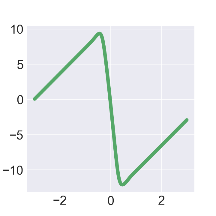
Fig. 2(b) shows the learned activation functions. We can integrate the learned activation functions (blue) to get the potential functions (green) used in our energy. For example the third potential function has the shape of a truncated Huber function. This means the function has learned to be robust against outliers.
5 Additional Qualitative Results
We use the supplementary material to show additional qualitative results of our method. The results shown in Figs. 4 and 3 impressively show how our simple denoising/refinement scheme is able to reconstruct high quality disparity maps.
The results on the Middlebury benchmark show, how information is exploited from both, the confidences and the input image to reconstruct the best possible disparity map. Note how the blue channel in Fig. 3 seems to be an indicator for regions being occluded, because they appear always next to left sided object boundaries.
As shown in Fig. 4 the results on Kitti show similar properties. Note here how fine details in the background are accurately captured. The confidence maps and the images guide the disparity map where discontinuities are likely to occur and where smoothing is the better option. The former is always close to object boundaries, and the latter is on the street, on cars or in the background.
