Emergence of second coherent regions for breathing chimera states

Abstract

Chimera states in one-dimensional nonlocally coupled phase oscillators are mostly assumed to be stationary, but breathing chimeras can occasionally appear, branching from the stationary chimeras via Hopf bifurcation. In this paper, we demonstrate two types of breathing chimeras: The type I breathing chimera looks the same as the stationary chimera at a glance, while the type II consists of multiple coherent regions with different average frequencies. Moreover, it is shown that the type I changes to the type II by increasing the breathing amplitude. Furthermore, we develop a self-consistent analysis of the local order parameter, which can be applied to breathing chimeras, and numerically demonstrate this analysis in the present system.

I Introduction

The collective dynamics of coupled nonlinear oscillators is beneficial for understanding a wide variety of scientific phenomena Kuramoto (1984); Pikovsky et al. (2003). Chimera states can result from a symmetry breaking in a large group of identical oscillators and have spatiotemporal patterns characterized by the coexistence of synchronized and desynchronized oscillators. Such a pattern was first discovered by Kuramoto and Battogtokh Kuramoto and Battogtokh (2002) in the one-dimensional array of nonlocally coupled complex Ginzburg-Landau (CGL) equations, which describe interacting biological cells Kuramoto (1995), and they introduced the self-consistent analysis of the local mean field by phase reduction. Then, the emergence of chimera states in the phase oscillators is characterized by two bifurcation parameters: the phase lag parameter, which is derived from the original parameters of the CGL equation, and the coupling range, which is given by the diffusion factor of substance mediating cellular interaction. Chimera states have actively been studied and have been found in various systems beyond the one-dimensional oscillator systems above Abrams and Strogatz (2004, 2006); Sethia et al. (2008); Laing (2009); Omel’chenko et al. (2010); Wolfrum and Omel’chenko (2011); Wolfrum et al. (2011); Omel’chenko (2013); Xie et al. (2014); Maistrenko et al. (2014); Panaggio and Abrams (2015); Smirnov et al. (2017); Bolotov et al. (2017, 2018); Suda and Okuda (2018); Omel’chenko (2018), with different coupling topologies Shima and Kuramoto (2004); Abrams et al. (2008); Pikovsky and Rosenblum (2008); Martens et al. (2010); Panaggio et al. (2016), different interaction functions Ashwin and Burylko (2015); Suda and Okuda (2015); Bick and Ashwin (2016), and different constituent oscillators Omelchenko et al. (2011, 2012, 2013); Schmidt et al. (2014); Schmidt and Krischer (2015); Omelchenko et al. (2015); Dai et al. (2017). The emergence of chimera states has also been reported experimentally Hagerstrom et al. (2012); Tinsley et al. (2012); Martens et al. (2013); Rosin et al. (2014).

When Kuramoto and Battogtokh Kuramoto and Battogtokh (2002) introduced the self-consistent analysis of the local mean field for chimera states, they assumed that the local mean field is time independent on the rotating frame of the whole oscillation. This means that the chimera state is collectively stationary. This assumption has been used in most studies of chimeras in the one-dimensional phase oscillator system and forms the basis of the analytical theory Kuramoto and Battogtokh (2002); Abrams and Strogatz (2004, 2006); Sethia et al. (2008); Omel’chenko (2013); Xie et al. (2014); Smirnov et al. (2017); Bolotov et al. (2017, 2018); Suda and Okuda (2018); Omel’chenko (2018).

A natural question arising from this assumption is whether nonstationary chimeras exist in the one-dimensional phase oscillator system Abrams et al. (2008). As an answer to this question, it is reported that breathing (oscillating) chimeras can be obtained by introducing phase lag parameter heterogeneity Laing (2009); Bolotov et al. (2017, 2018). On the other hand, we recently found that breathing chimeras can appear even without introducing such heterogeneity Suda and Okuda (2018). In these previous works, it is shown that the system exhibits a Hopf bifurcation from a stationary chimera to a breathing one.

In this paper, we study breathing chimeras in more detail. In Sec. II, we show that two types of breathing chimeras can be obtained by numerical simulations. The type I breathing chimera looks the same as the stationary chimera at a glance, as reported in Ref. Suda and Okuda (2018), while the type II has multiple coherent regions with different average frequencies. In Sec. III, we analyze these breathing chimeras by deriving a self-consistency equation extended for breathing chimeras and introducing a complex function combining the average frequency and the stability property. In Sec. IV, we show that the breathing chimera can be changed from type I to type II by increasing the breathing amplitude, and then new coherent regions appear in the incoherent regions for the type I. In Sec. V, we numerically solve this self-consistency equation.

II Numerical Simulation

We consider the one-dimensional array of nonlocally coupled phase oscillators in the continuum limit $N\to\infty$, where $N$ is the number of oscillators. The evolution equation of the system is given by

$$\dot{\theta}(x,t)=\omega-\int^{\pi}_{-\pi}dy\,G(x-y)\sin[\theta(x,t)-\theta(y,t)+\alpha],$$ (1)

with $2\pi$-periodic phase $\theta(x,t)\in[-\pi,\pi)$ on the space $x\in[-\pi,\pi)$ under the periodic boundary condition. The constant $\omega$ denotes the natural frequency. The interaction between oscillators is described as the sine function with the phase lag parameter $\alpha$ Sakaguchi and Kuramoto (1986). As the kernel $G(x)$ characterizing the nonlocal coupling, we use the step kernel Omel’chenko et al. (2010); Wolfrum and Omel’chenko (2011); Wolfrum et al. (2011); Omel’chenko (2013); Maistrenko et al. (2014); Suda and Okuda (2015, 2018); Omel’chenko (2018)

$$G(x)=\begin{cases}1/(2\pi r)&(|x|\leq\pi r)\\ 0&(|x|>\pi r),\end{cases}$$ (2)

with $0<r\leq 1$ where $r$ denotes the coupling range. The coupling kernel is usually given by an even real function and can be taken as, instead of the step kernel, the exponential kernel Kuramoto and Battogtokh (2002); Sethia et al. (2008); Smirnov et al. (2017); Bolotov et al. (2017, 2018) or the cosine kernel Abrams and Strogatz (2004, 2006); Laing (2009); Xie et al. (2014). For numerical simulations, we discretize $x$ into $x_{j}:=-\pi+2\pi j/N$ ($j=0,\cdots,N-1$) and rewrite Eqs. (1) and (2) as

$$\dot{\theta}_{j}(t)=\omega-\frac{1}{2R}\sum_{k=j-R}^{j+R}\sin[\theta_{j}(t)-\theta_{k}(t)+\alpha],$$ (3)

where $\theta_{j}(t):=\theta(x_{j},t)$, $R:=rN/2$ and the index $k$ is modulo $N$. For all the simulations of Eq. (3), we set $\omega=0$ without loss of generality and use the fourth-order Runge-Kutta method with time interval $\Delta t=0.01$.

Chimera states for Eq. (1) are characterized by the coexistence of coherent and incoherent regions. For example, Fig. 1 shows a chimera state with two coherent and incoherent regions. In the coherent region, the oscillators are synchronized with each other at a constant average frequency, while the oscillators in the incoherent region are drifting at continuously varying average frequencies. The average frequency is numerically defined as

$$\langle\dot{\theta}(x,t)\rangle:=\frac{1}{T}\int_{0}^{T}dt^{\prime}\,\dot{\theta}(x,t^{\prime}),$$ (4)

with the measurement time $T$ after a sufficiently long transient time. In the following, $\langle\cdot\rangle$ denotes the time average quantity.

Figure 1: Stationary chimera state with two coherent and incoherent regions for Eq. (3) with $N=100000$, $\alpha=1.480$, and $r=0.440$. (a) The snapshot of the phase $\theta(x,t)$. (b) The profile of the average frequency $\langle\dot{\theta}(x,t)\rangle$ with $T=2000$. (c) Time evolution of the global order parameter $|Z(t)|$. Figures (a) and (b) are plotted once every 10 oscillators.

While the chimera state in Fig. 1 is a stationary state, we have found breathing chimeras with two coherent and incoherent regions Suda and Okuda (2018), as shown in Fig. 2, which we call the type I breathing chimera below. Though the stationary and the type I breathing chimeras have very similar appearance of the phase snapshot, they can be distinguished by observing the time evolution of the global order parameter $|Z(t)|$, defined as

$$Z(t):=\frac{1}{2\pi}\int^{\pi}_{-\pi}dy\,e^{i\theta(y,t)},$$ (5)

which denotes the synchronization degree of all the oscillators. For $|Z(t)|=1$, all the oscillators are completely synchronized in phase, and otherwise for $0\leq|Z(t)|<1$. In the present case, $|Z(t)|$ becomes nearly zero for both of the stationary and the type I breathing chimeras, but the time evolutions are different. For stationary chimeras, $|Z(t)|$ is time-independent. Figure 1(c) denotes a small fluctuation around zero and can be regarded as nearly satisfying $|Z(t)|=0$. For breathing chimeras with sufficiently large $N$, however, $|Z(t)|$ oscillates periodically, as shown in Fig. 2(c).

Figure 2: The type I breathing chimera for Eq. (3) with $N=100000$, $\alpha=1.480$, and $r=0.360$. All figures show the same quantities as those in Fig. 1.

In our simulations of Eq. (3), the stationary and the type I breathing chimeras with two coherent and incoherent regions are obtained in the orange region in Fig. 3. In our previous work Suda and Okuda (2018), we showed that the breathing chimera branches from the stationary one via supercritical Hopf bifurcation. The bifurcation points are indicated by black solid lines in Fig. 3. We previously showed only the bifurcation points at $r\simeq 0.400$ by the linear stability analysis of the stationary chimera Suda and Okuda (2018). However, we have found the other bifurcation points at $r\simeq 0.580$ by the same method as before. Breathing chimeras are also found in two interacting populations of globally coupled phase oscillators, where the global order parameter of a desynchronized population oscillates temporally Abrams et al. (2008); Panaggio et al. (2016).

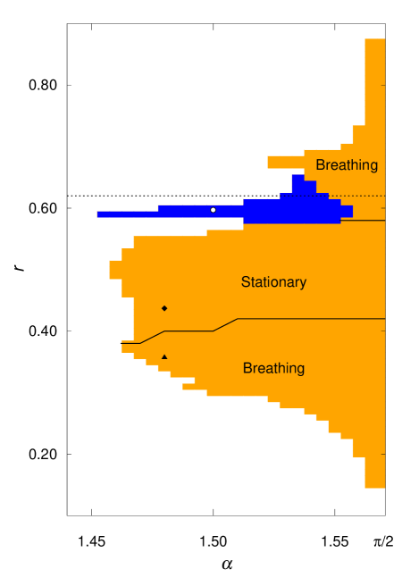
Figure 3: Stability region of chimera states obtained by the numerical simulation of Eq. (3). There appear the stationary and the type I breathing chimeras in the orange region and the type II breathing chimeras in the blue region. Black solid lines denote the Hopf bifurcation points Suda and Okuda (2018). The black diamond, the black triangle, and the white circle denote the parameter values of Figs. 1, 2, and 4, respectively. The horizontal dotted line denotes the parameter $r=0.620$ discussed in Sec. IV.

In addition to the type I breathing chimera, we have numerically found the type II breathing chimera characterized by two kinds of coherent regions with different average frequencies, as shown in Fig. 4. The first coherent regions around $x=0$ and $x=\pm\pi$ in Fig. 4(a) are similar to the coherent regions of the stationary or the type I breathing chimera; that is, they are always separated from each other by the phase almost exactly $\pi$. The second coherent regions lie near each first coherent region and have a different average frequency from it. Such type II breathing chimeras with multiple coherent regions are also observed in the system with phase lag parameter heterogeneity Bolotov et al. (2017, 2018). The stability region of the type II breathing chimeras is shown as the blue region in Fig. 3. In our numerical simulations, we did not find the bistable region of the types I and II. In this paper, we focus on these two types of breathing chimeras and aim to understand them theoretically.

Figure 4: The type II breathing chimera for Eq. (3) with $N=100000$, $\alpha=1.500$, and $r=0.600$. All figures show the same quantities as those in Fig. 1.

III Theory of Breathing Chimeras

In this section, we study the properties common to the two types of breathing chimeras. First, we define the local order parameter and the local mean field. The local order parameter Xie et al. (2014)

$$z(x,t):=\lim_{\eta\to 0+}\frac{1}{2\eta}\int^{x+\eta}_{x-\eta}dy\,e^{i\theta(y,t)},$$ (6)

which satisfies $0\leq|z(x,t)|\leq 1$, is similar to the global order parameter given by Eq. (5) in quality, and $|z(x,t)|$ denotes the synchronization degree of oscillators in the neighborhood of a point $x$. In the case of chimera states, $|z(x,t)|=1$ implies that the oscillator at $x$ belongs to a coherent region, and otherwise an incoherent region. We assume that the number of oscillators contained in the integral of Eq. (6) tends to infinity in the continuum limit $N\to\infty$. The local mean field Kuramoto and Battogtokh (2002) is defined as

$$Y(x,t):=\int^{\pi}_{-\pi}dy\,G(x-y)\,e^{i\theta(y,t)}.$$ (7)

Then, Eq. (1) is rewritten as

$$\dot{\theta}(x,t)=\omega-{\rm Im}[e^{i\alpha}e^{i\theta(x,t)}Y^{*}(x,t)],$$ (8)

where the symbol $*$ denotes the complex conjugate. Equation (8) suggests a physical picture in which each independent phase oscillator is driven by the local mean field $Y(x,t)$. Using the local order parameter $z(x,t)$, Eqs. (5) and (7) are rewritten as

$$Z(t)=\int^{\pi}_{-\pi}dy\,z(y,t),$$ (9)

$$Y(x,t)=\int^{\pi}_{-\pi}dy\,G(x-y)\,z(y,t).$$ (10)

In the continuum limit, phase oscillators described as Eq. (8) can be regarded as interacting subpopulations of globally coupled infinite oscillators in the neighborhood of $x$ Wolfrum et al. (2011). Then, we can obtain the evolution equation of $z(x,t)$ as

$$\dot{z}(x,t)=i\omega z(x,t)+\frac{1}{2}e^{-i\alpha}Y(x,t)-\frac{1}{2}e^{i\alpha}z^{2}(x,t)Y^{*}(x,t),$$ (11)

by the method in Refs. Pikovsky and Rosenblum (2008); Wolfrum et al. (2011) using the Watanabe-Strogatz approach Watanabe and Strogatz (1994). We can also define the local order parameter by using a probability density function of phase Laing (2009); Omel’chenko (2013, 2018). In that case, Eq. (11) can be obtained from the Ott-Antonsen ansatz Ott and Antonsen (2008, 2009).

If chimera states are stationary, the local order parameter takes the form

$$z(x,t)=z_{\rm st}(x)\,e^{i\Omega t},$$ (12)

with the frequency $\Omega$ of the rotating frame, which we may regard as the definition of “stationary” for chimera states. Then, the local mean field is also obtained as

$$Y(x,t)=Y_{\rm st}(x)\,e^{i\Omega t},$$ (13)

from Eq. (10). Using Eqs. (12) and (13), Eq. (11) is rewritten as

$$0=i\Delta z_{\rm st}(x)+\frac{1}{2}e^{-i\alpha}Y_{\rm st}(x)-\frac{1}{2}e^{i\alpha}z_{\rm st}^{2}(x)Y_{\rm st}^{*}(x),$$ (14)

where $\Delta:=\omega-\Omega$. When Eq. (14) is regarded as a quadratic equation with respect to $z_{\rm st}(x)$, the stable solution satisfying $0\leq|z(x,t)|\leq 1$ is

$$z_{\rm st}(x)=e^{-i\alpha}[i\Delta-g(x)]/Y_{\rm st}^{*}(x),$$ (15)

$$g(x):=\begin{cases}-|\Delta|\sqrt{(|Y_{\rm st}(x)|/\Delta)^{2}-1}&[|\Delta|\leq|Y_{\rm st}(x)|]\\ i\Delta\sqrt{1-(|Y_{\rm st}(x)|/\Delta)^{2}}&[|\Delta|>|Y_{\rm st}(x)|],\end{cases}$$ (16)

where $|\Delta|\leq|Y_{\rm st}(x)|$ and $|\Delta|>|Y_{\rm st}(x)|$ correspond to coherent and incoherent regions, respectively, and in Eq. (38) we confirm that this solution in Eq. (15) satisfies the local stability condition. Moreover, taking its convolution with the coupling kernel $G(x)$, we can obtain the self-consistency equation of $Y_{\rm st}(x)$ as

$$Y_{\rm st}(x)=e^{-i\alpha}\int^{\pi}_{-\pi}dy\,G(x-y)[i\Delta-g(y)]/Y_{\rm st}^{*}(y),$$ (17)

which agrees with the equation derived by Kuramoto and Battogtokh Kuramoto and Battogtokh (2002).

For breathing chimeras, instead of Eq. (12), we assume that the local order parameter takes the form

$$z(x,t)=\sum_{k=-\infty}^{\infty}z_{k}(x)\,e^{i(\Omega+k\delta)t},$$ (18)

introducing the breathing frequency $\delta$ in addition to the frequency $\Omega$ of the rotating frame. We take the sign of $\delta$ in accordance with $\Delta$; for example, when $\Delta>0$, we set $\delta>0$. Then,

$$Y(x,t)=\sum_{k=-\infty}^{\infty}Y_{k}(x)\,e^{i(\Omega+k\delta)t},$$ (19)

$$Y_{k}(x)=\int^{\pi}_{-\pi}dy\,G(x-y)\,z_{k}(y),$$ (20)

are also obtained from Eq. (10). Equation (18) is equivalent to the Fourier expansion of $z(x,t)$ and includes the stationary solution where $z_{0}(x)=z_{\rm st}(x)$ and $z_{k\neq 0}(x)=0$. Substituting Eqs. (18) and (19) into Eq. (11), we obtain the following equation for each $k$:

$$0 = i\Delta_{k}z_{k}(x)+\frac{1}{2}e^{-i\alpha}Y_{k}(x)$$ (21)

$$-\frac{1}{2}e^{i\alpha}{\displaystyle\sum_{l+m-n=k}}z_{l}(x)z_{m}(x)Y_{n}^{*}(x),$$

where $\Delta_{k}:=\omega-\Omega-k\delta$. Similarly to stationary chimeras, we also regard Eq. (21) as a quadratic equation with respect to $z_{k}(x)$ and obtain the solution

$$z_{k}(x)=[B_{k}(x)+\{{B_{k}}^{2}(x)-A_{k}(x)C_{k}(x)\}^{\frac{1}{2}}]/A_{k}(x),$$ (22)

$$A_{k}(x):=e^{i\alpha}Y_{k}^{*}(x),$$ (23)

$$B_{k}(x):=i\Delta_{k}-e^{i\alpha}\sum_{l\neq k}z_{l}(x)Y_{l}^{*}(x),$$ (24)

$$C_{k}(x):=-e^{-i\alpha}Y_{k}(x)+e^{i\alpha}\sum_{\begin{subarray}{c}l\neq k\\ m\neq k\end{subarray}}z_{l}(x)z_{m}(x)Y_{l+m-k}^{*}(x).$$ (25)

As the argument of the square root in Eq. (22), either one should be chosen to satisfy $|z(x,t)|\leq 1$ and the stability condition of the oscillator if it belongs to a coherent region. We can regard Eqs. (22)-(25) as the new self-consistency equations of the set of the complex coefficient function $\{z_{k}(x)\}$ for breathing chimeras, which are discussed in Sec. V.

The average frequency of breathing chimeras can be obtained by using Eq. (18). To simplify the notation, we describe the right-hand side of Eq. (6) as $\mathcal{P}e^{i\theta}$ with an operator $\mathcal{P}$ below. $\mathcal{P}A$ means that the function $A(x)$ is averaged in the neighborhood of a point $x$, that is,

$$(\mathcal{P}A)(x):=\lim_{\eta\to 0+}\frac{1}{2\eta}\int^{x+\eta}_{x-\eta}dy\,A(y).$$ (26)

We note that the continuous functions, e.g., $Y(x)$, are not affected by $\mathcal{P}$. Operating $\mathcal{P}$ on Eq. (8), we have

$$(\mathcal{P}\,\dot{\theta})(x,t)=\omega-{\rm Im}[e^{i\alpha}z(x,t)\,Y^{*}(x,t)].$$ (27)

Note that the right-hand side of Eq. (27) agrees with the other equation obtained by the Watanabe-Strogatz approach together with Eq. (11) (see Eq. (11) in Ref. Pikovsky and Rosenblum (2008)). Averaging both sides of Eq. (27) temporally, since $\mathcal{P}$ and $\langle\cdot\rangle$ are commutative, we have

$$\langle\dot{\theta}(x,t)\rangle=\omega-{\rm Im}[e^{i\alpha}\langle z(x,t)\,Y^{*}(x,t)\rangle].$$ (28)

Moreover, because

$$\langle z(x,t)\,Y^{*}(x,t)\rangle=\sum_{k=-\infty}^{\infty}z_{k}(x)\,Y_{k}^{*}(x),$$ (29)

is established for a sufficiently long measurement time, from Eq. (28) we obtain the average frequency as the imaginary part of the complex function

$$f(x):=i\omega-e^{i\alpha}\sum_{k=-\infty}^{\infty}z_{k}(x)\,Y_{k}^{*}(x).$$ (30)

Figures 5(a) and 5(b) show the profiles of the imaginary part of Eq. (30) corresponding to the average frequencies in Figs. 2(b) and 4(b). All figures in Fig. 5 are depicted by computing $z_{k}(x)$ and $Y_{k}(x)$ for $k\in[-5,5]$ in the numerical simulation of Eq. (3), and then we have computed $z_{k}(x)$ and $Y_{k}(x)$ as

$$z_{k}(x)=\langle e^{i\theta(x,t)}e^{-i(\Omega+k\delta)t}\rangle,$$ (31)

$$Y_{k}(x)=\langle Y(x,t)e^{-i(\Omega+k\delta)t}\rangle,$$ (32)

using the inverse transformation of Eqs. (18) and (19), where $\Omega$ and $\delta$ are computed from the Fourier transform of the time series $Z(t)$ by using Eqs. (9) and (18).

Figure 5: Profile of Eq. (30) for the type I [(a) and (c)] and the type II [(b) and (d)] breathing chimeras corresponding to Figs. 2 and 4, respectively. [(a), (b)] The imaginary part denotes the average frequency. [(c), (d)] The real part denotes the linear stability against a small local perturbation, where it is negative in stable coherent regions and zero in neutral incoherent regions. All figures are depicted by computing $z_{k}(x)$ and $Y_{k}(x)$ for $k\in[-5,5]$ obtained by the numerical simulation of Eq. (3).

In addition to the average frequency, we note that the real part of Eq. (30) denotes an important property of breathing chimeras, that is, the linear stability against a small local perturbation. Suppose that only the oscillator at $x$ is perturbed from $\theta(x,t)$ to $\theta(x,t)+\phi(x,t)$, where $\phi$ is small. Then, we are allowed to regard the local mean field $Y(x,t)$ as unchanged by that perturbation, as far as the continuum limit is considered, since the perturbation at only one point $x$ does not affect the integrated value $Y(x,t)$ in that limit. From Eq. (8), we can obtain the linear evolution equation of $\phi(x,t)$ as

$$\dot{\phi}(x,t)=[\partial_{\theta}V(\theta,x)]\,\phi(x,t),$$ (33)

$$\partial_{\theta}V(\theta,x)=-{\rm Re}[e^{i\alpha}e^{i\theta}Y^{*}(x,t)],$$ (34)

where $V(\theta,x)$ denotes the right-hand side of Eq. (8). When our breathing chimera is stable, the time-averaged $\langle\partial_{\theta}V(\theta,x)\rangle$ should be nonpositive. We act with the operator $\mathcal{P}$ on Eq. (34) and average the result over time, as Eqs. (27) and (28). Moreover, using Eq. (29), we finally obtain

$$\langle\partial_{\theta}V(\theta,x)\rangle=-{\rm Re}[e^{i\alpha}\sum_{k=-\infty}^{\infty}z_{k}(x)\,Y_{k}^{*}(x)],$$ (35)

which is equivalent to the real part of Eq. (30). Here, we assumed that $\langle\partial_{\theta}V(\theta,x)\rangle$ is a continuous function with respect to $x$, namely, which is not affected by $\mathcal{P}$. Figures 5(c) and 5(d) show the profiles of the real part of Eq. (30). In the coherent regions, the real part of Eq. (30) is negative, while that is zero in the incoherent regions. This implies that the oscillators are locally stable in the coherent regions and neutral in the incoherent regions.

For stationary chimeras, Eq. (30) is

$$f(x)=i\omega-e^{i\alpha}z_{\rm st}(x)\,Y_{\rm st}^{*}(x).$$ (36)

From Eqs. (15) and (16), we obtain $f(x)=i\Omega+g(x)$, therefore

$${\rm Im}f(x)=\begin{cases}\Omega&[|\Delta|\leq|Y_{\rm st}(x)|]\\ \Omega+\Delta\sqrt{1-(|Y_{\rm st}(x)|/\Delta)^{2}}&[|\Delta|>|Y_{\rm st}(x)|],\end{cases}$$ (37)

which agrees with the average frequency derived by Kuramoto and Battogtokh Kuramoto and Battogtokh (2002). The stability property is also obtained as

$${\rm Re}f(x)=\begin{cases}-|\Delta|\sqrt{(|Y_{\rm st}(x)|/\Delta)^{2}-1}&[|\Delta|\leq|Y_{\rm st}(x)|]\\ 0&[|\Delta|>|Y_{\rm st}(x)|].\end{cases}$$ (38)

We note that the set of $g(x)$ and its complex conjugate is the essential spectrum obtained by the linear stability analysis of the stationary chimera Omel’chenko (2013, 2018).

IV Relation between Two Types of Breathing Chimeras

Next, we study the relation between the two types of breathing chimeras in this section. In particular, we fix the parameter $r=0.620$, which corresponds to the horizontal dotted line in Fig. 3, and compare the two types of breathing chimeras with close parameters. For the numerical simulation of Eq. (3) with fixed $r=0.620$, the emergence of the types I and II is switched at $\alpha\simeq 1.550$; namely, the type I is stable for $1.550<\alpha<\pi/2$ and the type II for $\alpha<1.550$.

By the linear stability analysis of the stationary chimera Omel’chenko (2013); Xie et al. (2014); Smirnov et al. (2017); Bolotov et al. (2017, 2018); Suda and Okuda (2018); Omel’chenko (2018), the eigenvalues characterizing the stability of the stationary chimera can be obtained as the essential spectrum and the point spectrum. Then, the essential spectrum is given by the set of $g(x)$ [described as Eq. (16)] and its complex conjugate, which consists of pure imaginary and negative real eigenvalues, and the point spectrum determines whether the stationary chimera is stable. Figure 6 shows an example of the eigenvalues $\lambda$ for an unstable stationary chimera state obtained by the numerical method in Ref. Suda and Okuda (2018), where we computed the eigenvalues from the finite (but large) sized linearized matrix obtained by discretizing the space coordinate of Eq. (11). The point spectrum is a pair of the complex conjugate eigenvalues with a positive real value and the imaginary values about $\pm 0.215$. Though there are eigenvalues with positive real values around the real axis, they belong to the fluctuation of the essential spectrum by finite discretization of the numerical method, and approach zero by finer discretization Suda and Okuda (2018).

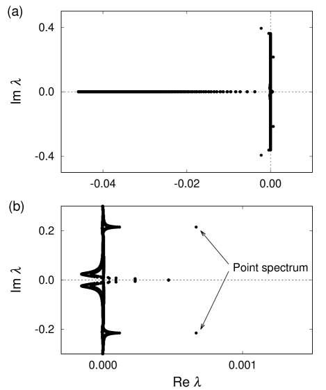
Figure 6: Complex eigenvalues $\lambda$ for the unstable stationary chimera state with $\alpha=1.549$ and $r=0.620$. (a) All eigenvalues. (b) The enlarged view of panel (a). The dashed lines in each panel are drawn only for reference.

We numerically computed these spectra for fixed $r=0.620$, and obtained results such that the positive real part of the point spectrum becomes larger continuously as $\alpha$ decreases around $\alpha\simeq 1.550$, as shown in Fig. 7. According to the analytical result in the neighborhood of a Hopf bifurcation point (see pages 8-13 in Ref. Kuramoto (1984)), we may expect that the amplitude of the limit-cycle solution gradually increases as the real part of such eigenvalues increases. Strictly speaking, the method in Ref. Kuramoto (1984) may not be applied to the present spectral problem, because the method in Ref. Kuramoto (1984) assumes that the linearized matrix of the system is finite-dimensional but the present problem has a continuous spectrum. We again refer to this problem in Sec. VI. Below, we will see that this increase of the amplitude causes the change of the type I breathing chimera to the type II.

Figure 7: Transition of the point spectrum with a positive imaginary value for fixed $r=0.620$. The square, the triangle, the circle, and the cross denote the point spectrum for $\alpha=1.551$, $\alpha=1.550$, $\alpha=1.549$, and $\alpha=1.548$, respectively. The dashed line is the imaginary axis.

As mentioned in Sec. II, we have found the Hopf bifurcation points at $r\simeq 0.400$ and $r\simeq 0.580$ between the stationary chimera and the type I breathing chimera by the linear stability analysis. Then, the absolute values of the imaginary parts of the point spectrum are nearly equal to the breathing frequency $\delta$ Suda and Okuda (2018). This agrees with the occurrence of a supercritical Hopf bifurcation. Therefore, for the type I breathing chimeras with a small breathing amplitude immediately after a Hopf bifurcation, we can assume that the local order parameter $z(x,t)$ given by Eq. (18) satisfies

$$z_{k}(x)=O(\epsilon^{|k|}),$$ (39)

where $\epsilon$ is a small bifurcation parameter Kuramoto (1984). Then, the local mean field $Y(x,t)$ also satisfies

$$Y_{k}(x)=O(\epsilon^{|k|}),$$ (40)

from Eq. (10). For $k=0$, substituting Eqs. (39) and (40) into Eq. (22) and eliminating the $O(\epsilon^{1})$ terms, Eq. (22) is equivalent to the stationary case Eqs. (15) and (16), where $A_{0}=e^{i\alpha}Y_{0}^{*}(x)$, $B_{0}=i\Delta_{0}$, and $C_{0}=e^{-i\alpha}Y_{0}(x)$. Therefore, we have

$$z_{0}(x)\simeq z_{\rm st}(x),\qquad Y_{0}(x)\simeq Y_{\rm st}(x),$$ (41)

where $z_{\rm st}(x)$ and $Y_{\rm st}(x)$ denote the quantities for the unstable stationary chimera at the same parameters that remains after the Hopf bifurcation of the stable stationary chimera. These agree with the numerical result as shown in Fig. 8. $Y_{0}(x)$ of the type I breathing chimera obtained by the numerical simulation of Eq. (3) and the numerical solution $Y_{\rm st}(x)$ to the self-consistency equation (17) look identical.

Figure 8: Local mean field of the type I breathing chimera and the stationary chimera. Figures show (a) the amplitude and (b) the argument. Open circles denote $Y_{0}(x)$ of the type I breathing chimera obtained by the numerical simulation of Eq. (3) with $N=100000$, $\alpha=1.551$, and $r=0.620$. Those circles are plotted once every $2000$ oscillators. The solid line denotes the numerical solution $Y_{\rm st}(x)$ to the self-consistency equation (17) at the same parameters. This solution corresponds to the unstable stationary chimera.

On the rotating frame with the frequency $\Omega$, $z(x,t)$ oscillates around the center $z_{0}(x)$, and $z_{k}(x)\,e^{ik\delta t}$ for $k=\pm 1$ are the main terms of oscillation for the type I breathing chimera. Substituting Eqs. (39) and (40) into Eq. (22) for $k=\pm 1$ and eliminating the $O(\epsilon^{2})$ terms, we obtain

$$z_{\pm 1}(x)\simeq\frac{-e^{-i\alpha}Y_{\pm 1}(x)+e^{i\alpha}{z_{0}}^{2}(x)Y_{\mp 1}^{*}(x)}{2[i\Delta_{\pm 1}-e^{i\alpha}z_{0}(x)Y_{0}^{*}(x)]}.$$ (42)

$z_{\pm 1}(x)$ are in the order of $\epsilon^{1}$ for almost all $x$, but in the vicinity of $x_{s}$ they become larger than $O(\epsilon)$ and therefore do not satisfy Eq. (42), if there exist specific points $x=x_{s}$ satisfying

$$i(\Omega+k\delta)=i\omega-e^{i\alpha}z_{0}(x)Y_{0}^{*}(x),$$ (43)

for $k=\pm 1$, since the denominator of the right-hand side in Eq. (42) becomes zero. From Eq. (41), the right-hand side of Eq. (43) agrees with Eq. (30) for the unstable stationary chimera in the order of $\epsilon^{0}$. In incoherent regions, Eq. (30) is purely imaginary and its imaginary part corresponds to the average frequency, as mentioned in Sec. III. Let us consider the case of $\Delta>0$. For stationary chimeras, the average frequency of the coherent region is equal to $\Omega$, which is the minimum value of the average frequency, from Eq. (37). Since $\delta>0$, if $\Omega+\delta$ is within the range between the maximum and the minimum of the average frequency, some points $x_{s}$ satisfying Eq. (43) for $k=1$ should exist. On the other hand, if $\Delta<0$, $\Omega$ is the maximum value of the average frequency. Then, some $x_{s}$ satisfying Eq. (43) for $k=1$ exist under the same condition of $\Omega+\delta$ since $\delta<0$. Therefore, from Eq. (37), if the breathing frequency $\delta$ satisfies the condition

$$0<|\delta|\leq{\rm max}\{|\Delta\sqrt{1-(|Y_{\rm st}(x)|/\Delta)^{2}}|\},$$ (44)

in incoherent regions ($\Delta>|Y_{\rm st}(x)|$), some specific points $x_{s}$ exist, and $|z_{1}(x_{s})|$ becomes larger sharply than other points $x$. We note that $|z_{1}(x_{s})|$ does not diverge to infinity. The function $z_{\pm 1}(x)$ is determined by Eq. (22), but can be approximately found by Eq. (42) for all $x\in[-\pi,\pi)$ such that the denominator in Eq. (42) is separated from zero. At $x=x_{s}$, the denominator in Eq. (42) for $k=1$ is zero. Then, $z_{\pm 1}(x_{s})$ does not obey Eq. (42). However, the correct values of $z_{\pm 1}(x_{s})$ still can be found from Eq. (22), and $|z_{1}(x_{s})|$ practically becomes a large finite value. In our numerical simulations ($\omega=0$) presented here, we observed $\Delta>0$ and therefore Eq. (44) becomes

$$0<\delta\leq\Delta\,(=-\Omega),$$ (45)

since the minimum of $|Y_{\rm st}(x)|$ is zero as shown in Fig. 8.

From the existence of specific points $x_{s}$, we can explain that the type I changes to the type II by increasing the breathing amplitude, as follows. After the Hopf bifurcation from stationary chimeras, there appear the type I breathing chimeras with a small breathing amplitude. This amplitude is mainly characterized by $z_{\pm 1}(x)$, which are very small for almost $x$. However, $z_{1}(x)$ is large only at $x_{s}$. As increasing the breathing amplitude by leaving the bifurcation point, $z_{\pm 1}(x)$ gradually becomes large. By the increase in $z_{\pm 1}(x)$, especially $z_{1}(x_{s})$, $z(x,t)$ reaches the upper limit $|z(x,t)|=1$ at $x_{s}$, e.g., for $\alpha\simeq 1.550$ and $r=0.620$. When $\alpha$ decreases further from $\alpha=1.550$ with fixed $r=0.620$, $z_{1}(x_{s})$ cannot become large anymore. Instead, the second coherent regions with average frequency $\Omega+\delta$ emerge around $x_{s}$ with increasing the amplitude; in other words, the type II breathing chimera appears.

Let us confirm this scenario by numerical simulations of Eq. (3). Figure 9 shows comparison between the two types of breathing chimeras near the bifurcation between them. For the type I breathing chimera for $r=0.620$ and $\alpha=1.551$ (see the left column in Fig. 9), we obtained $\Omega\simeq-0.3602$ and $\delta\simeq 0.2151$, then from Eq. (43) we can see that $\langle\dot{\theta}(x_{s},t)\rangle=\Omega+\delta$ is established for $k=1$ at, e.g., $x_{s}\simeq 0.705$. Such a profile as $|z_{1}(x)|$ nearly diverges can often be seen just before the bifurcation to the type II. As shown in Fig. 9(g), $|z_{1}(x)|$ is very small for almost all $x$ but nearly diverges at the points $x_{s}$.

Figure 9: Comparison between the two types of breathing chimeras for the numerical simulation of Eq. (3) with $N=100000$ and $r=0.620$. The left column denotes the type I for $\alpha=1.551$, and the right column denotes the type II for $\alpha=1.549$. Figures (a) and (b) show the snapshot of the phase. Figures (c) and (d) show the profile of the average frequency. Figures (e) and (f) and figures (g) and (h) show the amplitudes of $z_{0}(x)$ and $z_{1}(x)$, respectively. All the figures are plotted once every $10$ oscillators. Note that the appearance of the types I and II is switched at $\alpha\simeq 1.550$.

For the type II breathing chimeras, the local order parameter does not satisfy Eq. (39), because $z_{0}(x)$ as shown in Fig. 9(f) clearly differs from $z_{\rm st}(x)$ [$\simeq z_{0}(x)$ for the type I]; that is, Eq. (41) is not satisfied. Therefore, it turns out that the breathing amplitude for type II is larger than that for type I. When Figs. 9(a) and 9(b) are compared, we find that a part of the incoherent region suddenly changes to the second coherent region. Then, it is observed that the second coherent regions for type II emerge at the same points as $x_{s}$ for type I and have the average frequency $\Omega+\delta$ obtained from the simulation results $\Omega\simeq-0.3974$ and $\delta\simeq 0.2067$. From this result, our scenario is shown to be valid. As shown in Fig. 3, we do not observe that the type I breathing chimeras for $r<0.400$ change to the type II. This seems to be because the amplitude increase is smaller than that for $r>0.600$.

For $|k|\geq 2$, we can obtain $z_{k}(x)$ of the order of $\epsilon^{|k|}$ similar to Eq. (42) and the same condition as Eq. (43). Therefore, there can also exist special points $x_{s}$ satisfying Eq. (43), if $\Omega+k\delta$ is within the range between the maximum and minimum of the average frequency. In other words, if the breathing frequency $\delta$ satisfies the condition

$$0<k|\delta|\leq{\rm max}\{|\Delta\sqrt{1-(|Y_{\rm st}(x)|/\Delta)^{2}}|\},$$ (46)

the type II breathing chimera has $(k+1)$-th coherent regions with the average frequency $\Omega+k\delta$. In the present case, $\delta$ does not satisfies Eq. (46) except for $k=1$, so the type II breathing chimeras cannot have the third and greater coherent regions. However, the type II breathing chimeras in Refs. Bolotov et al. (2017, 2018) appear to have the second and third coherent regions, though the system used in Refs. Bolotov et al. (2017, 2018) includes phase lag parameter heterogeneity. We emphasize that our analytical theory and scenario can be applied to the system with phase lag parameter heterogeneity only by replacing $\alpha$. As mentioned above, $|\delta|$ is nearly equal to the absolute value of the imaginary parts of the point spectrum in the neighborhood of a Hopf bifurcation point. Therefore, when the type I breathing chimera is bifurcated via Hopf bifurcation, it is already determined whether the type II breathing chimera has the second or greater coherent regions.

V Self-Consistent Analysis

Finally, we propose a self-consistent analysis for breathing chimeras. As mentioned in Sec. III, Eqs. (22)-(25) are the self-consistency equations of $\{z_{k}(x)\}$. In this section, we numerically solve them, especially, for the type II breathing chimera.

Equations. (22)-(25) are composed of one complex equation for every $k$. Therefore, we need two additional conditions to obtain the solution because there are unknown complex functions $\{z_{k}(x)\}$ and two real unknowns $\Omega$ and $\delta$ to be determined. Unlike the breathing chimeras, the self-consistency equation (17) for stationary chimeras has one unknown complex function $Y_{\rm st}(x)$ and one real unknown $\Omega$, and an additional condition obtained from the invariance of Eq. (17) under any rotation of the argument of $Y_{\rm st}(x)$ leads to solving the self-consistency equationAbrams and Strogatz (2004, 2006); Sethia et al. (2008); Xie et al. (2014); Suda and Okuda (2018); for example, ${\rm Arg}[Y_{\rm st}(0)]=0$ is chosen.

Equation. (30) can be utilized for obtaining the additional real conditions to determine $\Omega$ and $\delta$. The average frequencies of the first and second coherent regions are equal to $\Omega$ and $\Omega+\delta$, respectively. Moreover, the coherent region satisfies the stability condition ${\rm Re}f(x)<0$, and ${\rm Re}f(x)$ has a minimal value in every coherent region, as shown in Fig. 5. Let $x_{c1}$ and $x_{c2}$ be the minimal points of ${\rm Re}f(x)$ corresponding to the first and second coherent regions, respectively. Then, the frequencies $\Omega$ and $\delta$ are given by

$$\Omega={\rm Im}f(x_{c1}),$$ (47)

$$\delta={\rm Im}f(x_{c2})-{\rm Im}f(x_{c1}).$$ (48)

Note that Eq. (47) is also established for stationary chimeras. In the following, we regard Eqs. (22)-(25) and Eqs. (47) and (48) as the complete self-consistency equations for the type II breathing chimeras.

There are a few important points to solve the self-consistency equations numerically. First, we truncate $\{z_{k}(x)\}$ to $k\in[-10,10]$, assuming that $z_{k}(x)$ for sufficiently large $|k|$ is small enough not to affect the other $z_{k}(x)$. That is confirmed from the results of the numerical simulation of Eq. (3).

The second point is the selection method of the argument of the square root in Eq. (22). Equation. (22) can produce two solutions according to this selection. In our numerical computation of the two solutions for all $k$, we have found that the orders of these two solutions are greatly different except for the first coherent regions for $k=0$ and the second coherent regions for $k=1$. In that case, the larger one is easily rejected because of the condition $|z(x,t)|<1$. The problem is the exceptional case where the orders of the two solutions are not so different. Then, one of the two solutions corresponds to the stable solution and the other does not. That can be shown as follows. Because Eqs. (22)-(25) are transformed to

$$\{{B_{k}}^{2}(x)-A_{k}(x)C_{k}(x)\}^{\frac{1}{2}} = -i\Delta_{k}+e^{i\alpha}\sum_{k=-\infty}^{\infty}z_{k}(x)\,Y_{k}^{*}(x),$$ (49)

$$= i(\Omega+k\delta)-f(x),$$

where $f(x)$ is the same function in Eq. (30), we have

$$f(x)=i(\Omega+k\delta)-\{{B_{k}}^{2}(x)-A_{k}(x)C_{k}(x)\}^{\frac{1}{2}}.$$ (50)

It is interesting that the right-hand side of Eq. (50) should be independent of $k$. Therefore, since ${\rm Im}f(x)=\Omega$ in the first coherent regions, the square root becomes the real number for $k=0$, and either one corresponding to ${\rm Re}f(x)<0$ should be selected from the stability in the coherent regions. The case in the second coherent regions for $k=1$ is the same as above.

In this way, we can select the stable solution to Eq. (22) at almost all $x$ for $k=0,1$. However, the stable and unstable solutions are too close to be distinguished around the boundaries between the coherent and incoherent regions since ${\rm Re}f(x)\simeq 0$. To solve this problem, we use the following method. For example, let us consider the boundaries between the first coherent and incoherent regions for $k=0$. Substituting Eq. (49) into Eqs. (22)-(25), we have

$$z_{k}(x)=[B_{k}(x)+i(\Omega+k\delta)-f(x)]/A_{k}(x).$$ (51)

This equation is also derived from Eq. (30) directly. Because the branch of the square root for $k\neq 0$ is easily selected by the orders of the two solutions, the right-hand side of Eq. (50) can be computed for a specific $k\neq 0$. When it is difficult to distinguish the two solutions for $k=0$, we may use Eq. (50) for $k\neq 0$ as $f(x)$ in Eq. (51).

Figure 10: Local order parameter of the type II breathing chimera for $\alpha=1.500$ and $r=0.600$ corresponding to Fig. 4. Figures show the amplitude of (a) $z_{0}(x)$, (b) $z_{1}(x)$, and (c) $z_{-1}(x)$. Open circles denote the values obtained by the numerical simulation of Eq. (3) with $N=100000$, and are plotted once every $2000$ oscillators. The solid line denotes the numerical solution to the self-consistency equations (22)-(25), (47), and (48).

Figure 10 shows numerical solutions to the self-consistency equations (22)-(25), (47), and (48). At first, we tried to numerically solve the self-consistency equations by the simple iteration method, where unknown variables $\{z_{k}(x)\}$, $\Omega$, and $\delta$ are substituted into the right-hand side of the equations and are regenerated from the left-hand side. However, we could not obtain a solution of the type II breathing chimeras because the variables have not converged even by using various initial conditions. Instead, we have applied Steffensen’s method Steffensen (1933) to the regeneration of every variable and have succeeded in obtaining the correct numerical solution. Open circles in Fig. 10 denote $z_{k}(x)$ obtained by the numerical simulation of Eq. (3). We used them as the initial condition for solving the self-consistency equations. The results from the numerical simulation and the self-consistency equations look like almost identical. Although it may seem that they are not identical in a part of $|z_{1}(x)|$, that is caused by the numerical error due to the finite-size effects of the simulations. We expect that more extensive simulations improve this discrepancy. We succeeded in obtaining the solution to the self-consistency equations by using an initial condition that is very close to the correct solution. However, when other initial conditions were used, the correct solution could not be obtained since the variables have not converged. This may be a weak point of our numerical method.

VI Summary

We have studied breathing chimera states in one-dimensional nonlocally coupled phase oscillators. First, we have found breathing chimeras in numerical simulations. The breathing chimeras are characterized by the temporally oscillating global order parameter and classified into two types by observing the average frequencies of the coherent regions. While type I contains the coherent regions with a common average frequency similarly to the stationary chimera, type II contains the coherent regions with different average frequencies. Type II breathing chimeras are also obtained for Eq. (1) with phase lag parameter heterogeneity Bolotov et al. (2017, 2018).

Next, we have assumed that the local order parameter $z(x,t)$ takes the form of Eq. (18) instead of Eq. (12) as in many previous works, and analytically discussed breathing chimeras. Moreover, we have derived the self-consistency equations (22)-(25) and the important complex function Eq. (30), whose imaginary and real parts denote the average frequency and the local linear stability, respectively. They turns out to be very useful to analyze breathing chimeras.

We have shown that the type I breathing chimera changes to type II by increasing the breathing amplitude. This means that the type I breathing chimera looks the same as the stationary chimera since the breathing amplitude is small but the second coherent regions emerge in the incoherent regions as that amplitude becomes larger. Such a bifurcation, that new coherent regions emerge in the incoherent regions, has been reported in a few systems that are different from phase oscillators Omelchenko et al. (2013); Dai et al. (2017). However, the mechanism of that bifurcation in the other systems is unclear.

In the present paper, we applied the analytical result in Ref. Kuramoto (1984) to the spectral problem corresponding to the linearization of Eq. (11). However, this method may not rigorously be justified in $N\to\infty$. To understand breathing chimera states more precisely, we need to analyze them by a more sophisticated perturbation theory for infinite-dimensional systems Kato (1995).

Finally, we have numerically solved the self-consistency equations (22)-(25). Then, the frequencies $\Omega$ and $\delta$ are formulated as Eqs. (47) and (48), respectively. Our numerical method has succeeded in solving them, but it is necessary to use the initial condition that is very close to the correct solution. To obtain the solution more easily, we need to improve the present method in future.

References

- Kuramoto (1984) Y. Kuramoto, Chemical Oscillation, Waves, and Turbulence (Springer, Berlin, 1984).
- Pikovsky et al. (2003) A. Pikovsky, M. Rosenblum, and J. Kurths, Synchronization: A Universal Concept in Nonlinear Sciences (Cambridge University Press, Cambridge, 2003).
- Kuramoto and Battogtokh (2002) Y. Kuramoto and D. Battogtokh, Nonlinear Phenom. Complex Syst. 5, 380 (2002).
- Kuramoto (1995) Y. Kuramoto, Prog. Theor. Phys. 94, 321 (1995).
- Abrams and Strogatz (2004) D. M. Abrams and S. H. Strogatz, Phys. Rev. Lett. 93, 174102 (2004).
- Abrams and Strogatz (2006) D. M. Abrams and S. H. Strogatz, Int. J. Bifurc. Chaos 16, 21 (2006).
- Sethia et al. (2008) G. C. Sethia, A. Sen, and F. M. Atay, Phys. Rev. Lett. 100, 144102 (2008).
- Laing (2009) C. R. Laing, Physica D 238, 1569 (2009).
- Omel’chenko et al. (2010) O. E. Omel’chenko, M. Wolfrum, and Y. L. Maistrenko, Phys. Rev. E 81, 065201 (2010).
- Wolfrum and Omel’chenko (2011) M. Wolfrum and O. E. Omel’chenko, Phys. Rev. E 84, 015201 (2011).
- Wolfrum et al. (2011) M. Wolfrum, O. E. Omel’chenko, S. Yanchuk, and Y. L. Maistrenko, Chaos 21, 013112 (2011).
- Omel’chenko (2013) O. E. Omel’chenko, Nonlinearity 26, 2469 (2013).
- Xie et al. (2014) J. Xie, E. Knobloch, and H.-C. Kao, Phys. Rev. E 90, 022919 (2014).
- Maistrenko et al. (2014) Y. L. Maistrenko, A. Vasylenko, O. Sudakov, R. Levchenko, and V. L. Maistrenko, Int. J. Bifurc. Chaos 24, 1440014 (2014).
- Panaggio and Abrams (2015) M. J. Panaggio and D. M. Abrams, Nonlinearity 28, R67 (2015).
- Smirnov et al. (2017) L. Smirnov, G. Osipov, and A. Pikovsky, J. Phys. A 50, 08LT01 (2017).
- Bolotov et al. (2017) M. I. Bolotov, L. A. Smirnov, G. V. Osipov, and A. S. Pikovsky, JETP Lett. 106, 393 (2017).
- Bolotov et al. (2018) M. Bolotov, L. Smirnov, G. Osipov, and A. Pikovsky, Chaos 28, 045101 (2018).
- Suda and Okuda (2018) Y. Suda and K. Okuda, Phys. Rev. E 97, 042212 (2018).
- Omel’chenko (2018) O. E. Omel’chenko, Nonlinearity 31, R121 (2018).
- Shima and Kuramoto (2004) S.-i. Shima and Y. Kuramoto, Phys. Rev. E 69, 036213 (2004).
- Abrams et al. (2008) D. M. Abrams, R. Mirollo, S. H. Strogatz, and D. A. Wiley, Phys. Rev. Lett. 101, 084103 (2008).
- Pikovsky and Rosenblum (2008) A. Pikovsky and M. Rosenblum, Phys. Rev. Lett. 101, 264103 (2008).
- Martens et al. (2010) E. A. Martens, C. R. Laing, and S. H. Strogatz, Phys. Rev. Lett. 104, 044101 (2010).
- Panaggio et al. (2016) M. J. Panaggio, D. M. Abrams, P. Ashwin, and C. R. Laing, Phys. Rev. E 93, 012218 (2016).
- Ashwin and Burylko (2015) P. Ashwin and O. Burylko, Chaos 25, 013106 (2015).
- Suda and Okuda (2015) Y. Suda and K. Okuda, Phys. Rev. E 92, 060901 (2015).
- Bick and Ashwin (2016) C. Bick and P. Ashwin, Nonlinearity 29, 1468 (2016).
- Omelchenko et al. (2011) I. Omelchenko, Y. Maistrenko, P. Hövel, and E. Schöll, Phys. Rev. Lett. 106, 234102 (2011).
- Omelchenko et al. (2012) I. Omelchenko, B. Riemenschneider, P. Hövel, Y. Maistrenko, and E. Schöll, Phys. Rev. E 85, 026212 (2012).
- Omelchenko et al. (2013) I. Omelchenko, O. E. Omel’chenko, P. Hövel, and E. Schöll, Phys. Rev. Lett. 110, 224101 (2013).
- Schmidt et al. (2014) L. Schmidt, K. Schönleber, K. Krischer, and V. García-Morales, Chaos 24, 013102 (2014).
- Schmidt and Krischer (2015) L. Schmidt and K. Krischer, Chaos 25, 064401 (2015).
- Omelchenko et al. (2015) I. Omelchenko, A. Zakharova, P. Hövel, J. Siebert, and E. Schöll, Chaos 25, 083104 (2015).
- Dai et al. (2017) Q. Dai, D. Liu, H. Cheng, H. Li, and J. Yang, PLoS ONE 12(10), e0187067 (2017).
- Hagerstrom et al. (2012) A. M. Hagerstrom, T. E. Murphy, R. Roy, P. Hövel, I. Omelchenko, and E. Schöll, Nat. Phys. 8, 658 (2012).
- Tinsley et al. (2012) M. R. Tinsley, S. Nkomo, and K. Showalter, Nat. Phys. 8, 662 (2012).
- Martens et al. (2013) E. A. Martens, S. Thutupalli, A. Fourriére, and O. Hallatschek, Proc. Natl. Acad. Sci. USA 110, 10563 (2013).
- Rosin et al. (2014) D. P. Rosin, D. Rontani, N. D. Haynes, E. Schöll, and D. J. Gauthier, Phys. Rev. E 90, 030902 (2014).
- Sakaguchi and Kuramoto (1986) H. Sakaguchi and Y. Kuramoto, Prog. Theor. Phys. 76, 576 (1986).
- Watanabe and Strogatz (1994) S. Watanabe and S. H. Strogatz, Physica D 74, 197 (1994).
- Ott and Antonsen (2008) E. Ott and T. M. Antonsen, Chaos 18, 037113 (2008).
- Ott and Antonsen (2009) E. Ott and T. M. Antonsen, Chaos 19, 023117 (2009).
- Steffensen (1933) J. F. Steffensen, Scand. Actuar. J. 1933, 64 (1933).
- Kato (1995) T. Kato, Perturbation Theory for Linear Operators (Springer, Berlin, Heidelberg, 1995).