Computing Abstract Distances in Logic Programs

Abstract

Abstract interpretation is a well-established technique for performing static analyses of logic programs. However, choosing the abstract domain, widening, fixpoint, etc. that provides the best precision-cost trade-off remains an open problem. This is in a good part because of the challenges involved in measuring and comparing the precision of different analyses. We propose a new approach for measuring such precision, based on defining distances in abstract domains and extending them to distances between whole analyses of a given program, thus allowing comparing precision across different analyses. We survey and extend existing proposals for distances and metrics in lattices or abstract domains, and we propose metrics for some common domains used in logic program analysis, as well as extensions of those metrics to the space of whole program analysis. We implement those metrics within the CiaoPP framework and apply them to measure the precision of different analyses over both benchmarks and a realistic program.

bstract interpretation, static analysis, logic programming, metrics, distances, complete lattices, program semantics.

1 Introduction

Many practical static analyzers for (Constraint) Logic Programming ((C)LP) are based on the theory of Abstract Interpretation [8]. The basic idea behind this technique is to interpret (i.e., execute) the program over a special abstract domain to obtain some abstract semantics of the program, which will over-approximate every possible execution in the standard (concrete) domain. This makes it possible to reason safely (but perhaps imprecisely) about the properties that hold for all such executions. As mentioned before, abstract interpretation has proved practical and effective for building static analysis tools, and in particular in the context of (C)LP [30, 21, 38, 6, 12, 5, 29, 16, 25].

Recently, these techniques have also been applied successfully to the analysis and verification of other programming paradigms by using (C)LP (Horn Clauses) as the intermediate representation for different compilation levels, ranging from source to bytecode or ISA  [1, 3, 33, 17, 26, 10, 19, 4, 28, 24].

When designing or choosing an abstract interpretation-based analysis, a crucial issue is the trade-off between cost and precision, and thus research in new abstract domains, widenings, fixpoints, etc., often requires studying this trade-off. However, while measuring analysis cost is typically relatively straightforward, having effective precision measures is much more involved. There have been a few proposals for this purpose, including, e.g., probabilistic abstract interpretation [13] and some measures in numeric domains [27, 37] , but they have limitations and in practice most studies come up with ad-hoc measures for measuring precision. Furthermore, there have been no proposals for such measures in (C)LP domains.

We propose a new approach for measuring the precision of abstract interpretation-based analyses in (C)LP, based on defining distances in abstract domains and extending them to distances between whole analyses of a given program, which allow comparison of precision across different analyses. Our contributions can be summarized as follows: We survey and extend existing proposals for distances in lattices and abstract domains (Sec. 3). We then build on this theory and ideas to propose distances for common domains used in (C)LP analysis (Sec. 3.2). We also propose a principled methodology for comparing quantitatively the precision of different abstract interpretation-based analyses of a whole program (Sec. 4). This methodology is parametric on the distance in the underlying abstract domain and only relies in a unified representation of those analysis results as AND-OR trees. Thus, it can be used to measure the precision of new fixpoints, widenings, etc. within a given abstract interpretation framework, not requiring knowledge of its implementation. To the extent of our knowledge, all previous principled attempts at measuring the precision of different abstract interpretations have addressed the precision of analysis operators, rather than providing a general methodology for comparing the results obtained for particular programs. Finally, we also provide experimental evidence about the appropriateness of the proposed distances (Sec. 5).

2 Background and Notation

Lattices:

A partial order on a set $X$ is a binary relation $\sqsubseteq$ that is reflexive, transitive, and antisymmetric. The greatest lower bound or meet of $a$ and $b$, denoted by $a\sqcap b$, is the greatest element in $X$ that is still lower than both of them ($a\sqcap b\sqsubseteq a,~{}a\sqcap b\sqsubseteq b,~{}(c\sqsubseteq a\ \land c\sqsubseteq b\implies c\sqsubseteq a\sqcap b))$. If it exists, it is unique. The least upper bound or join of $a$ and $b$, denoted by $a\sqcup b$, is the smallest element in $X$ that is still greater than both of them ($a\sqsubseteq a\sqcup b,~{}b\sqsubseteq a\sqcup b,~{}(a\sqsubseteq c\land b\sqsubseteq c\implies a\sqcup b\sqsubseteq c)$). If it exists, it is unique. A partially ordered set (poset) is a couple $(X,\sqsubseteq)$ such that the first element $X$ is a set and the second one is a partial order relation on $X$. A lattice is a poset for which any two elements have a meet and a join. A lattice $L$ is complete if, extending in the natural way the definition of supremum and infimum to subsets of $L$, every subset $S$ of $L$ has both a supremum $sup(S)$ and an infimum $inf(S)$. The maximum element of a complete lattice, $\sup(L)$ is called top or $\top$, and the minimum, $\inf(L)$ is called bottom or $\bot$.

Galois Connections:

Let $(L_{1},\sqsubseteq_{1})$ and $(L_{2},\sqsubseteq_{2})$ be two posets. Let $f:L_{1}\longrightarrow L_{2}$ and $g:L_{2}\longrightarrow L_{1}$ be two applications such that:

$$\forall x\in L_{1},y\in L_{2}:f(x)\,\sqsubseteq_{2}\,y\iff x\,\sqsubseteq_{1}\,g(y)$$

Then the quadruple $\langle L_{1},f,L_{2},g\rangle$ is a Galois connection, written $L_{1}\galois{f}{g}L_{2}$. If $f\circ g$ is the identity, then the quadruple is called a Galois insertion.

Abstract Interpretation and Abstract Domains:

Abstract interpretation [8] is a well-known static analysis technique that allows computing sound over-approximations of the semantics of programs. The semantics of a program can be described in terms of the concrete domain, whose values in the case of (C)LP are typically sets of variable substitutions that may occur at runtime. The idea behind abstract interpretation is to interpret the program over a special abstract domain, whose values, called abstract substitutions, are finite representations of possibly infinite sets of actual substitutions in the concrete domain. We will denote the concrete domain as $D$, and the abstract domain as $D_{\alpha}$. We will denote the functions that relate sets of concrete substitutions with abstract substitutions as the abstraction function $\alpha:D\longrightarrow D_{\alpha}$ and the concretization function $\gamma:D_{\alpha}\longrightarrow D$. The concrete domain is a complete lattice under the set inclusion order, and that order induces an ordering relation in the abstract domain herein represented by “$\sqsubseteq$.” Under this relation the abstract domain is usually a complete lattice or cpo and $(D,\alpha,D_{\alpha},\gamma)$ is a Galois insertion. The abstract domain is of finite height or alternatively it is equipped with a widening operator, which allows for skipping over infinite ascending chains during analysis to a greater fixpoint, achieving convergence in exchange for precision.

Metric:

A metric on a set $S$ is a function $d:S\times S\rightarrow\mathbb{R}$ satisfying:

• Non-negativity: $\forall x,y\in S,~{}d(x,y)\geq 0$.

• Identity of indiscernibles: $\forall x,y\in S,~{}d(x,y)=0\iff x=y$.

• Symmetry: $\forall x,y\in S,~{}d(x,y)=d(y,x)$.

• Triangle inequality: $\forall x,y,z\in S,~{}d(x,z)\leq d(x,y)+d(y,z)$.

A set $S$ in which a metric is defined is called a metric space. A pseudometric is a metric where two elements which are different are allowed to have distance 0. We call the left implication of the identity of indiscernibles, weak identity of indiscernibles. A well-known method to extend a metric $d:S\times S\longrightarrow\mathbb{R}$ to a metric in $\wp{(}S)$ is using the Hausdorff distance, defined as:

$$\text{d}_{H}(A,B)=\max\left\{\sup_{a\in A}\inf_{b\in B}\text{d}(a,b),\sup_{b\in B}\inf_{a\in A}\text{d}(a,b)\right\}$$

3 Distances in Abstract Domains

As anticipated in the introduction, our distances between abstract interpretation-based analyses of a program will be parameterized by distance in the underlying abstract domain, which we assume to be a complete lattice. In this section we propose a few such distances for relevant logic programming abstract domains. But first we review and extend some of the concepts that arise when working with lattices or abstract domains as metric spaces.

3.1 Distances in lattices and abstract domains

When defining a distance in a partially ordered set, it is necessary to consider the compatibility between the metric and the structure of the lattice. This relationship will suggest new properties that a metric in a lattice should satisfy. For example, a distance in a lattice should be order-preserving, that is, $\forall a,b,c\in D~{}with~{}a\sqsubseteq b\sqsubseteq c,~{}then~{}d(a,b),d(b,c)\leq d(a,c)$. It is also reasonable to expect that it fulfills what we have called the diamond inequality, that is, $\forall a,b,c,d\in D~{}with~{}c\sqcap d\sqsubset a\sqcap b,~{}a\sqcup b\sqsubset c\sqcup d,~{}then~{}d(a,b)\leq d(c,d)$. But more importantly, this relationship will suggest insights for constructing such metrics.

One such insight is precisely defining a partial metric $d_{\sqsubseteq}$ only between elements which are related in the lattice, which is arguably easier, and to extend it later to a distance between arbitrary elements $x,y$, as a function of $d_{\sqsubseteq}(x,x\sqcap y),~{}d_{\sqsubseteq}(y,x\sqcap y),~{}d_{\sqsubseteq}(x,x\sqcup y),~{}d_{\sqsubseteq}(x,x\sqcup y)$ and $d_{\sqsubseteq}(x\sqcap y,x\sqcup y)$. Jan Ramon et al. [36] show under which circumstances $d_{\sqsubseteq}(x,x\sqcup y)+d_{\sqsubseteq}(y,x\sqcup y)$ is a distance, that is, when $d_{\sqsubseteq}$ is order-preserving and fulfills $d_{\sqsubseteq}(x,x\sqcup y)+d_{\sqsubseteq}(y,x\sqcup y)\leq d_{\sqsubseteq}(x,x\sqcap y)+d_{\sqsubseteq}(y,x\sqcap y)$.

In particular, one could define a monotonic size $size:L\rightarrow\mathbb{R}$ in the lattice and define $d_{\sqsubseteq}(a,b)$ as $size(b)-size(a)$. Gratzer [18] shows that if the size fullfills $size(x)+size(y)=size(x\sqcap y)+size(x\sqcup y)$, then $d(x,y)=size(x\sqcup y)-size(x\sqcap y)$ is a metric. De Raedt [11] shows that $d(x,y)=size(x)+size(y)-2\cdot size(x\sqcup y)$ is a metric iff $size(x)+size(y)\leq size(x\sqcap y)+size(x\sqcup y)$, and an analogous result with $d(x,y)=size(x)+size(y)-2\cdot size(x\sqcup y)$ and $\geq$ instead of $\leq$. Note that the first distance is the equivalent of the symmetric difference distance in finite sets, with $\sqsubseteq$ instead of $\subseteq$ and $size$ instead of the cardinal of a set. Similar distances for finite sets, such as the Jaccard distance, can be translated to lattices in the same way. Another approach to defining $d_{\sqsubseteq}$ that follows from the idea of using the lattice structure, is counting the steps between two elements (i.e., the number of edges between both elements in the Hasse diagram of the lattice). This was used by Logozzo [27].

When defining a distance not just in any lattice, but in an actual abstract domain (abstract distance from now on), it is also necessary to consider the relation of the abstract domain with the concrete domain (i.e., the Galois connection), and how an abstract distance is interpreted under that relation. In that sense, we can observe that a distance $d_{D_{\alpha}}:D_{\alpha}\rightarrow D_{\alpha}$ in an abstract domain will induce a distance $d_{D}^{\alpha}:D\rightarrow D$ in the concrete one, as $d_{D}^{\alpha}(A,B)=d_{D_{\alpha}}(\alpha(A),\alpha(B))$, and the other way around: a distance $d_{D}:D\rightarrow D$ in the concrete domain induces an abstract distance $d_{D_{\alpha}}^{\gamma}:D_{\alpha}\rightarrow D_{\alpha}$ in the abstract one, as $d_{D_{\alpha}}^{\gamma}(a,b)=d_{D}(\gamma(a),\gamma(b))$. Thus, an abstract distance can be interpreted as an abstraction of a distance in the concrete domain, or as a way to define a distance in it, and it is clear that it is when interpreted that way that an abstract distance makes most sense from a program semantics point of view.

It is straightforward to see (and we show in the appendix) that these induced distances inherit most metric and order-related properties. In particular, if a distance $d_{D}$ in the concrete domain is a metric, its abstraction $d_{D_{\alpha}}$ is a pseudo-metric in the abstract domain, and a full metric if the Galois connection between $D$ and $D_{\alpha}$ is a Galois insertion. This allows us to define distances $d_{\alpha}$ in the abstract domain from distances $d$ the concrete domain, as $d_{\alpha}(a,b)=d(\gamma(a),\gamma(b))$. This approach might seem of little applicability, due to the fact that concretizations will most likely be infinite and we still need metrics in the concrete domain. But in the case of logic programs, such metrics for Herbrand terms already exist (e.g., [22, 34, 36]), and in fact we show later a distance for the regular types domain that can be interpreted as an extension of this kind, of the distance proposed by Nienhuys-Cheng [34] for sets of terms.

Finally, we note that a metric in the Cartesian product of lattices can be easily derived from existing distances in each lattice, for example as the 2-norm or any other norm of the vector of distances component to component. This is relevant because many abstract domains, such as those that are combinations of two different abstract domains, or non-relational domains which provide an abstract value from a lattice for each variable in the substitution, are of such form. However, although this is a well-known result, it is not clear whether the resulting distance will fulfill other lattice-related properties if the distances for each component do. It is straightforward to see that that is the case for the order-preserving property, but not for the diamond inequality, due to the fact that for abstract domains, all elements of the lattice $(a_{1},\ldots,a_{n})$ for which $\exists i~{}s.t.~{}a_{i}=\bot$ are identified as the bottom element of the cartesian product lattice, since their concretization is $\emptyset$.

3.2 Distances in Logic Programming Domains

We now propose some distances for two well-known abstract domains used in (C)LP, following the considerations presented in the previous section.

Sharing domain:

The sharing domain [23, 30] is a well-known domain for analyzing the sharing (aliasing) relationships between variables and grounding in logic programs. It is defined as $\wp(\wp(Pvar))$, that is, an abstract substitution for a clause is defined to be a set of sets of program variables in that clause, where each set indicates that the terms to which those variables are instantiated at runtime might share a free variable. More formally, we define $Occ(\theta,U)=\{X|X\in dom(\theta),U\in vars(X\theta)\}$, the set of all program variables $X\in Pvar$ in the clause such that the variable $U\in Uvar$ appears in $X\theta$. We define the abstraction of a substitution $\theta$ as ${\cal A}_{sharing}(\theta)~{}=~{}\{Occ(\theta,U)\;|\;U\in Uvar\}$, and extend it to sets of substitutions. The order induced by this abstraction in $\wp(\wp(Pvar))$ is the set inclusion, the join, the set union, and the meet, the set intersection. As an example, a program variable that does not appear in any set is guaranteed to be ground, two variables that never appear in the same set are guaranteed to not share, or $\top=\wp(Pvar)$. The complete definition can be found in [23, 30]).

Following the approach of previous section, we define this monotone size in the domain: $size(a)=|a|+1,size(\bot)=0$. It is straightforward to check that $\forall a,b\in Sh,~{}size(a)+size(b)=size(a\sqcap b)+size(a\sqcup b)$. Therefore the following distance is a metric and order-preserving:

$$d_{share}(Sh_{1},Sh_{2})=size(Sh_{1}\cup Sh_{2})-size(Sh_{1}\cap Sh_{2})=|(Sh_{1}\cup Sh_{2})|-|size(Sh_{1}\cap Sh_{2})|$$

We would like our distance to be in a normalized range $[0,1]$, and for that we divide it between $d(\bot,\top)=2^{n}$, where $n=|V|$ denotes the number of variables in the domain of the substitutions. This yields the following final distance, which is a metric by construction:

$$d_{share}(Sh_{1},Sh_{2})=(|(Sh_{1}\cup Sh_{2})|-|size(Sh_{1}\cap Sh_{2})|)/2^{n}$$

Regular-type domain:

Another well-known domain for logic programs is the regular types domain [9], which abstracts the shape or type of the terms to which variables are assigned on runtime. It associates each variable with a deterministic context free grammar that describes its shape, with the possible functors and atoms of the program as terminal symbols. A more formal definition can be found in [9]. We will write abstract substitutions as tuples $\langle T_{1},\ldots,T_{n}\rangle$, where $T_{i}=(S_{i},{\cal T}_{i},{\cal F}_{i},{\cal R}_{i})$ is the grammar that describes the term associated to the i-th variable in the substitution. We propose to use as a basis the Hausdorff distance in the concrete domain, using the distance between terms proposed in [34], i.e.,

$\\ \begin{array}[]{l}d_{term}(f(x_{1},\ldots,x_{n}),g(y_{1},\ldots,y_{m}))=\left\{\begin{array}[]{ll}if&f/n\neq g/m\;\;\;\;then\;\;1\\ else&p\sum_{i=1}^{n}{\frac{1}{n}d_{term}(x_{i},y_{i})}\end{array}\right.\end{array}\\$

As the derived abstract version, we propose the following distance between two types or grammars $S_{1},~{}S_{2}$, defined recursively and with a little abuse of notation:

$\begin{array}[]{l}d^{\prime}(S_{1},S_{2})=\left\{\begin{array}[]{ll}if&\exists~{}(S_{1}\rightarrow f(T_{1},\ldots,T_{n}))\in{\cal R}_{1}\land\nexists(S_{2}\rightarrow f(T^{\prime}_{1},\ldots,T^{\prime}_{n}))\in{\cal R}_{2}\;\;\;\;then\;\;1\\ if&\exists~{}(S_{2}\rightarrow f(T_{1},\ldots,T_{n}))\in{\cal R}_{2}\land\nexists(S_{1}\rightarrow f(T^{\prime}_{1},\ldots,T^{\prime}_{n}))\in{\cal R}_{1}\;\;\;\;then\;\;1\\ else&max\{p\sum_{i=1}^{n}{\frac{1}{n}d^{\prime}(T_{i},T^{\prime}_{i})}~{}|~{}(S_{1}\rightarrow f(T_{1},\ldots,T_{n}))\in{\cal R}_{1}\land\\ &~{}~{}~{}~{}~{}~{}~{}~{}~{}~{}~{}~{}~{}~{}~{}~{}~{}~{}~{}~{}~{}~{}~{}~{}~{}~{}~{}~{}~{}~{}~{}~{}~{}~{}~{}~{}~{}~{}~{}~{}~{}~{}~{}~{}~{}~{}~{}~{}~{}~{}~{}~{}~{}(S_{2}\rightarrow f(T^{\prime}_{1},\ldots,T^{\prime}_{n}))\in{\cal R}_{2}\}\end{array}\right.\end{array}\\$

We also extend this distance between types to distance between substitutions in the abstract domain as follows:

$d(\langle T_{1},\ldots,T_{n}\rangle,\langle T^{\prime}_{1},\ldots,T^{\prime}_{n}\rangle)=\sqrt{d^{\prime}(T_{1},T^{\prime}_{1})^{2}+\ldots+d^{\prime}(T_{n},T^{\prime}_{n})^{2}}$

Since $d^{\prime}$ is the abstraction of the Hausdorff distance with $d_{term}$, which it is proved to be a metric in [34], $d^{\prime}$ is a metric too, as seen in the previous section. Therefore $d$ is also a metric, since it is its extension to the cartesian product.

4 Distances between analyses

We now attempt to extend a distance in an abstract domain to distances between results of different abstract interpretation-based analyses of the same program over that domain. In the following we will assume (following most “top-down” analyzers for (C)LP programs [30, 5, 16, 25]) that the result of an analysis for a given entry (i.e., an initial predicate P, and an initial call pattern or abstract query $\lambda_{c}$), is an AND-OR tree, with root the OR-node $\langle P,\lambda_{c},\lambda_{s}\rangle_{\lor}$, where $\lambda_{s}$ is the abstract substitution computed by the analysis for that predicate given that initial call pattern. An AND-OR tree alternates AND-nodes, which correspond to clauses in the program, and OR-nodes, which correspond to literals in those clauses. An OR-node is a triplet $\langle L,\lambda_{c},\lambda_{s}\rangle_{\lor}$, with L a call to a predicate P and $\lambda_{c},\lambda_{s}$ the abstract call and success substitutions for that goal. It has one AND-node $\langle C_{j},\beta_{entry}^{j},\beta_{exit}^{j}\rangle_{\land}$ as child for each clause $C_{j}$ in the definition of P, where $\beta_{entry}^{j}=\lambda_{c}~{}\forall j$ and $\lambda_{s}=\bigsqcup\beta_{exit}^{j}$. An AND-node is a triplet $\langle C,\beta_{entry},\beta_{exit}\rangle_{\land}$, with C a clause $Head:-L_{1},...,L_{n}$ and with $\beta_{entry},\beta_{exit}$ the abstract entry and exit substitutions for that clause. It has an OR-node $\langle L_{i},\lambda_{c}^{i},\lambda_{s}^{i}\rangle_{\lor}$ for each literal $L_{i}$ in the clause, where $\beta_{entry}=\lambda_{c}^{1},~{}\lambda_{s}^{i}=\lambda_{c}^{i+1},~{}\lambda_{s}^{n}=\beta_{exit}$. This tree is the abstract counterpart of the resolution trees that represent concrete top-down executions, and represents a possibly infinite set of those resolution trees at once. The tree will most likely be infinite, but can be represented as a finite cyclic tree. We denote the children of a node $T$ as $ch(T)$.

Example 1

Let us consider as an example the simple quick-sort program (using difference lists) in Fig. 1, which uses an entry assertion to specify the initial abstract query of the analysis [35]. If we analyze it with a simple groundness domain (with just two values g and ng, plus $\top$ and $\bot$), the result can be represented with the graph shown in Fig. 1.

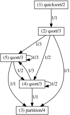
  ⬇ :- module(quicksort,[quicksort/2],[assertions]). :- use_module(partition,[partition/4]). :- entry quicksort(Xs,Ys) : (ground(Xs), var(Ys)). quicksort(Xs,Ys) :- qsort(Xs,Ys,[]). qsort([],Ys,Ys). qsort([X|Xs],Ys,TailYs) :- partition(Xs,X,L,R), qsort(R,R2,TailYs), qsort(L,Ys,[X|R2]). (1) $\langle quicksort(Xs,Ys),~{}~{}\{Xs/g,Ys/ng\},~{}~{}\{Xs/g,Ys/g\}\rangle$ (2) $\langle qsort(Xs,Ys,[]),~{}~{}\{Xs/g,Ys/ng\},~{}~{}\{Xs/g,Ys/g\}\rangle$ (3) $\langle partition(Xs,X,L,R),~{}~{}\{Xs/g,X/g,L/ng,R/ng\},~{}~{}\{Xs/g,X/g,L/g,R/g\}\rangle$ (4) $\langle qsort(Xs,Ys,Zs),~{}~{}\{Xs/g,Ys/ng,Zs/g\},~{}~{}\{Xs/g,Ys/g,Zs/g\}\rangle$ (5) $\langle qsort(Xs,Ys,[Z|Zs]),~{}~{}\{Xs/g,Ys/ng,Z/g,Zs/g\},~{}~{}\{Xs/g,Ys/g,Z/g,Zs/g\}\rangle$

Figure 1: Analysis of quicksort/2 (using difference lists).

That graph is a finite representation of an infinite abstract and-or tree. The nodes in the graph correspond to or-nodes $\langle L,\lambda^{c},\lambda^{s}\rangle$ in the analysis tree, where the literals $L$, abstract call substitutions $\lambda^{c}$ and abstract success substitutions $\lambda^{s}$ are specified below the graph. The labels in the edge indicate to which program point each node corresponds: if one node is connected to its predecessor by an arrow with label $i/j$, then that node corresponds to the $j$-th literal of the $i$-th clause of the predicate indicated by the predecessor. The and-nodes are left implicit. $\Box$

We propose three distances between AND-OR trees $S_{1},S_{2}$ for the same entry, in increasing order of complexity, and parameterized by a distance $d_{\alpha}$ in the underlying abstract domain. We also discuss which metric properties are inherited by these distances from $d_{\alpha}$. Note that a good distance for measuring precision should fulfill the identity of indiscernibles.

Top distance.

The first consists in considering only the roots of the top trees, $\langle P,\lambda_{c},\lambda_{s}^{1}\rangle_{\lor}$ and $\langle P,\lambda_{c},\lambda_{s}^{2}\rangle_{\lor}$, and defining our new distance as $d(S_{1},S_{2})=d_{\alpha}(\lambda_{s}^{1},\lambda_{s}^{2})$. This distance ignores too much information (e.g., if the entry point is a predicate main/0, the distance would only distinguish analyses that detect failure from analysis which do not), so it is not appropriate for measuring analysis precision, but it is still interesting as a baseline. It is straightforward to see that it is a pseudometric if $d_{\alpha}$ is, but will not fulfill the identity of indiscernibles even if $d_{\alpha}$ does.

Flat distance.

The second distance considers all the information inferred by the analysis for each program point, but forgetting about its context in the AND-OR tree. In fact, analysis information is often used this way, i.e., considering only the substitutions with which a program point can be called or succeeds, and not which traces lead to those calls (path insensitivity). We define a distance between program points

$$d_{PP}(S_{1},S_{2})=\frac{1}{2}(d_{\alpha}(\bigsqcup_{\lambda\in PP_{c}^{1}}\lambda,\bigsqcup_{\lambda\in PP_{c}^{2}}\lambda)+d_{\alpha}(\bigsqcup_{\lambda\in PP_{s}^{1}}\lambda,\bigsqcup_{\lambda\in PP_{s}^{2}}\lambda))$$

where $PP_{c}^{i}=\{\lambda_{c}~{}|~{}\langle PP,\lambda_{c},\lambda_{s}\rangle_{\lor}\in S_{i}\}$, $PP_{s}^{i}=\{\lambda_{s}~{}|~{}\langle PP,\lambda_{c},\lambda_{s}\rangle_{\lor}\in S_{i}\}$. If we denote $P$ as the set of all program points in the program, that distance can later be extended to a distance between analyses as $d(S_{1},S_{2})=\frac{1}{|P|}\sum_{PP\in P}d_{PP}(S_{1},S_{2})$, or any other combination of the distances $d_{PP}(S_{1},S_{2})$ (e.g, weighted average, $||\cdot||_{2}$). This distance is more appropriate for measuring precision than the previous one, but it will still inherit all metric properties except the identity of indiscernibles.

Tree distance.

For the third distance, we propose the following recursive definition, which can easily be translated into an algorithm:

$\\ \begin{array}[]{l}d(T_{1},T_{2})=\left\{\begin{array}[]{ll}\mu\frac{1}{2}(d_{\alpha}(\lambda_{c}^{1},\lambda_{c}^{2})+d_{\alpha}(\lambda_{s}^{1},\lambda_{s}^{2}))+(1-\mu)\frac{1}{|C|}\sum_{(c_{1},c_{2})\in C}d(c_{1},c_{2})~{}~{}~{}~{}~{}if~{}C\neq\emptyset\\ else~{}~{}~{}\frac{1}{2}(d_{\alpha}(\lambda_{c}^{1},\lambda_{c}^{2})+d_{\alpha}(\lambda_{s}^{1},\lambda_{s}^{2}))\end{array}\right.\end{array}\\$

where $T_{1}=\langle P,\lambda_{c}^{1},\lambda_{s}^{1}\rangle,~{}T_{2}=\langle P,\lambda_{c}^{2},\lambda_{s}^{2}\rangle,~{}\mu\in(0,1],~{}C_{1}=ch(T_{1}),~{}C_{2}=ch(T_{2})$ and $C=\{(c_{1},c_{2})~{}|~{}c_{1}\in ch(T_{1}),c_{2}\in ch(T_{2}),val(c_{1})=\langle X,\_,\_\rangle,val(c_{2})=\langle Y,\_,\_\rangle,X=Y\}$. This definition is possible because the two AND-OR trees will necessarily have the same shape, and therefore we are always comparing a node with its correspondent node in the other tree. Also, this distance is well defined, even if the trees, and therefore the recursions, are infinite, since the expression above always converges. Furthermore, the distance to which the expression converges can be easily computed in finite time. Since the AND-OR trees always have a finite representation as cyclic trees with $n$ and $m$ nodes respectively, there are at most $n*m$ different pairs of nodes to visit during the recursion. Assigning a variable to each pair that is actually visited, the recursive expression can be expressed as a linear system of equations. That system has a unique solution since the original expression had, but also because there is an equation for each variable and the associated matrix, which is therefore squared, has strictly dominant diagonal. An example can be found in the appendix 0.B.2.

The idea of this distance is that we consider more relevant the distance between the upper nodes than the distance between the deeper ones, but we still consider all of them and do not miss any of the analysis information. As a result, this distance will directly inherit the identity of indiscernibles (apart from all other metric properties) from $d_{\alpha}$.

5 Experimental Evaluation

To evaluate the usefulness of the program analysis distances, we set up a practical scenario in which we study quantitatively the cost and precision tradeoff for several abstract domains. In order to do it we need to overcome two technical problems described below.

Base domain.

Recall that in the distances defined so far, we assume that we compare two analyses using the same abstract domain. We relax this requirement by translating each analysis to a common base domain, rich enough to reflect a particular program property of interest. An abstract substitution $\lambda$ over a domain $D_{\alpha}$ is translated to a new domain $D_{\alpha^{\prime}}$ as $\lambda^{\prime}$ = $\alpha^{\prime}(\gamma(\lambda))$, and the AND-OR tree is translated by just translating any abstract substitution occurring in it. The results still over-approximates concrete executions, but this time all over the same abstract domain.

Program analysis intersection.

Ideally we would compare each analysis with the actual semantics of a program for a given abstract query, represented also as an AND-OR tree. However, this semantics is undecidable in general, and we are seeking an automated process. Instead, we approximated it as the intersection of all the computed analyses. The intersection between two trees, which can be easily generalized to $n$ trees, is defined as $inter(T_{1},T_{2})=T$, with

$$val(T_{1})=\langle X,\lambda_{c}^{1},\lambda_{s}^{2}\rangle,~{}val(T_{2})=\langle X,\lambda_{c}^{2},\lambda_{s}^{2}\rangle,~{}val(T)=\langle X,\lambda_{c}^{1}\sqcap\lambda_{c}^{2},\lambda_{s}^{1}\sqcap\lambda_{s}^{2}\rangle$$

$$ch(T)=\{inter(c_{1},c_{2})~{}|~{}c_{1}\in ch(T_{1}),c_{2}\in ch(T_{2}),val(c_{1})=\langle X,\_,\_\rangle,val(c_{2})=\langle Y,\_,\_\rangle,X=Y\}$$

That is, a new AND-OR tree with the same shape as those computed by the analyses, but where each abstract substitution is the greatest lower bound of the corresponding abstract substitutions in the other trees. The resulting tree is the least general AND-OR tree we can obtain that still over-approximates every concrete execution.

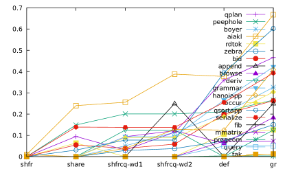
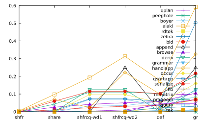
Figure 2: (a) Precision using flat distance and (b) tree distance (micro-benchmarks)

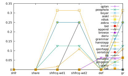
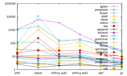
Figure 3: (a) Precision using top distance and (b) Analysis time (micro-benchmarks)

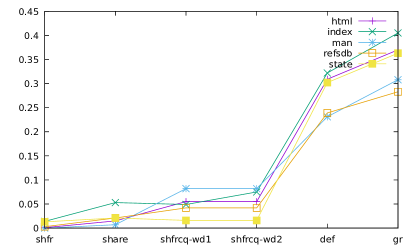
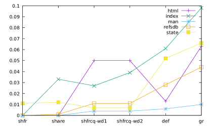
Figure 4: (a) Precision using flat distance and (b) tree distance (LPdoc benchmark)

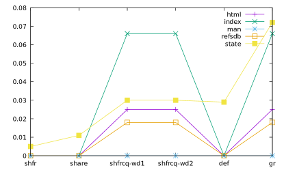
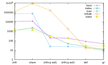
Figure 5: (a) Precision using top distance and (b) Analysis time (LPdoc benchmarks)

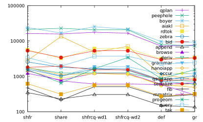
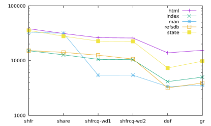
Figure 6: (a) Analysis size (micro-benchmarks) and (b) Analysis size (LPdoc benchmark)

Case study: variable sharing domains.

We have applied the method above on a well known set of (micro-)benchmarks for CLP analysis, and a number of modules from a real application (the LPdoc documentation generator). The programs are analyzed using the CiaoPP framework [20] and the domains shfr [31], share [23, 30], def [15, 2], and sharefree_clique [32] with different widenings. All these domains express sharing between variables among other things, and we compare them with respect to the base share domain. All experiments are run on a Linux machine with Intel Core i5 CPU and 8GB of RAM.

Fig. 2 and Fig. 3 show the results for the micro-benchmarks. Fig. 4 and Fig. 5 show the same experiment on LPdoc modules. In both experiments we measure the precision using the flat distance, tree distance, and top distance. In general, the results align with our a priori knowledge: that shfr is strictly more precise than all other domains, but also generally slower; while gr is less precise and faster. As expected, the flat and tree distances show that share is in all cases less precise than shfr, and not significantly cheaper (sometimes even more costly). The tree distance shows a more pronounced variation of precision when comparing share and widenings. While this can also be appreciated in the top distance, the top distance fails to show the difference between share and shfr. Thus, the tree distance seems to offer a good balance. For small programs where analysis requires less than 100ms in shfr, there seems to be no advantage in using less precise domains. Also as expected, for large programs widenings provide significant speedups with moderate precision lose. Small programs do not benefit in general from widenings. Finally, the def domain shows very good precision w.r.t. the top distance, representing that the domain is good enough to capture the behavior of predicates at the module interface for the selected benchmarks.

Fig. 6 reflects the size of the AND-OR tree and experimentally it is correlated with the analysis time. The size measures of representing abstract substitutions as Prolog terms (roughly as the number of functor and constant symbols).

6 Related Work

Distances in lattices: Lattices and other structures that arise from order relations are common in many areas of computer science and mathematics, so it is not surprising that there have been already some attempts at proposing metrics in them. E.g., [18] has a dedicated chapter for metrics in lattices. Distances among terms: Hutch [22], Nienhuys-Cheng [34] and Jan Ramon [36] all propose distances in the space of terms and extend them to distances between sets of terms or clauses. Our proposed distance for regular types can be interpreted as the abstraction of the distance proposed by Nienhuys-Cheng. Furthermore, [36] develop some theory of metrics in partial orders, as also does De Raedt [11]. Distances among abstract elements and operators: Logozzo [27] proposes defining metrics in partially ordered sets and applying them to quantifying the relative loss of precision induced by numeric abstract domains. Our work is similar in that we also propose a notion of distance in abstract domains. However, they restrict their proposed distances to finite or numeric domains, while we focus instead on logic programming-oriented, possible infinite, domains. Also, our approach to quantifying the precision of abstract interpretations follows quite different ideas. They use their distances to define a notion of error induced by an abstract value, and then a notion of error induced by a finite abstract domain and its abstract operators, with respect to the concrete domain and concrete operators. Instead, we work in the context of given programs, and quantify the difference of precision between the results of different analyses for those programs, by extending our metrics in abstract domains to metrics in the space of abstract executions of a program and comparing those results. Sotin [37] defines measures in $\mathbb{R}^{n}$ that allow quantifying the difference in precision between two abstract values of a numeric domain, by comparing the size of their concretizations. This is applied to guessing the most appropriate domain to analyse a program, by under-approximating the potentially visited states via random testing and comparing the precision with which different domains would approximate those states. Di Pierro [13] proposes a notion of probabilistic abstract interpretation, which allows measuring the precision of an abstract domain and its operators. In their proposed framework, abstract domains are vector spaces instead of partially ordered sets, and it is not clear whether every domain, and in particular those used in logic programming, can be reinterpreted within that framework. Cortesi [7] proposes a formal methodology to compare qualitatively the precision of two abstract domains with respect to some of the information they express, that is, to know if one is strictly more precise that the other according to only part of the properties they abstract. In our experiments, we compare the precision of different analyses with respect to some of the information they express. For some, we know that one is qualitatively more precise than the other in Cortesi’s paper’s sense, and that is reflected in our results.

7 Conclusions

We have proposed a new approach for measuring and comparing precision across different analyses, based on defining distances in abstract domains and extending them to distances between whole analyses. We have surveyed and extended previous proposals for distances and metrics in lattices or abstract domains, and proposed metrics for some common (C)LP domains. We have also proposed extensions of those metrics to the space of whole program analysis. We have implemented those metrics and applied them to measuring the precision of different sharing-related (C)LP analyses on both benchmarks and a realistic program. We believe that this application of distances is promising for debugging the precision of analyses and calibrating heuristics for combining different domains in portfolio approaches, without prior knowledge and treating domains as black boxes (except for the translation to the base domain). In the future we plan to apply the proposed concepts in other applications beyond measuring precision in analysis, such as studying how programming methodologies or optimizations affect the analyses, comparing obfuscated programs, giving approximate results in semantic code browsing [14], program synthesis, software metrics, etc.

Acknowledgements: Research partially funded by EU FP7 agreement no 318337 ENTRA, Spanish MINECO TIN2015-67522-C3-1-R TRACES project, the Madrid M141047003 N-GREENS program and BLOQUES-CM project, and the TEZOS Foundation TEZOS project.

Appendix 0.A Theory of Section 3

0.A.1 Properties inherited by abstraction or concretization of distances

Proposition 1

Let us consider an abstract domain $D_{\alpha}$, that abstracts the concrete domain $D$, with abstraction function $\alpha:D\rightarrow D_{\alpha}$ and concretization function $\gamma:D_{\alpha}\rightarrow D$. Both domains are complete lattices and $\alpha$ and $\gamma$ form a Galois connection. Then:

(1) If $d_{\alpha}:D_{\alpha}\times D_{\alpha}\rightarrow\mathbb{R}$ is a metric in the abstract domain, then $d:D\times D\rightarrow\mathbb{R},~{}d(A,B)=d_{\alpha}(\alpha(A),\alpha(B))$ is a pseudometric in the concrete domain. If $d_{\alpha}$ is order-preserving, so it is $d$.

(2) If $d:D\times D\rightarrow\mathbb{R}$ is a metric in the concrete domain, then $d_{\alpha}:D_{\alpha}\times D_{\alpha}\rightarrow\mathbb{R},~{}d_{\alpha}(a,b)=d(\gamma(a),\gamma(b))$ is a pseudometric in the abstract domain. If the Galois connection is a Galois insertion, then $d$ is a full metric. If $d$ is order-preserving, so it is $d_{\alpha}$.

Proof (Proof)

• (1)

  • $d$ is a pseudometric:

    • Non-negativity: $d(A,B)=d_{\alpha}(\alpha(A),\alpha(B))\geq 0$, since $d_{\alpha}$ is non-negative
      

    • Weak identity of indiscernibles : $d(A,A)=d_{\alpha}(\alpha(A),\alpha(A))=0$, since $d_{\alpha}$ fulfills the identity of indiscernibles
      

    • Symmetry: $d(A,B)=d_{\alpha}(\alpha(A),\alpha(B))=d_{\alpha}(\alpha(B),\alpha(A))=d(B,A)$, since $d_{\alpha}$ is symmetric
      

    • Triangle inequality: $d(A,C)=d_{\alpha}(\alpha(A),\alpha(C))\leq d_{\alpha}(\alpha(A),\alpha(B))+d_{\alpha}(\alpha(B),\alpha(C))=d(A,B)+d(B,C)$, since $d_{\alpha}$ fulfills the triangle inequality
      

  • $d$ is order-preserving:

    If $A\subseteq B\subseteq C$, then $\alpha(A)\sqsubseteq\alpha(B)\sqsubseteq\alpha(C)$, since $\alpha$ is monotonic. But then $d(A,B)=d_{\alpha}(\alpha(A),\alpha(B))\leq d_{\alpha}(\alpha(A),\alpha(C))=d(A,C)$, since $d_{\alpha}$ is order-preserving.

• (2)

  • $d_{\alpha}$ is a pseudometric: analogous. Besides, if the Galois connection is a Galois insertion, then $\gamma$ is injective (otherwise, $\exists~{}a\neq b\in D_{\alpha}~{}s.t.~{}\gamma(a)=\gamma(b)\implies\alpha(\gamma(a))=\alpha(\gamma(b))\implies a=b$, which is absurd). But then $d_{\alpha}(a,b)=0\implies d(\gamma(a),\gamma(b))=0\implies\gamma(a)=\gamma(b)\implies a=b$, and therefore $d_{\alpha}$ is a full metric

  • $d_{\alpha}$ is order-preserving: Analogous

Appendix 0.B Examples for section 4

0.B.1 Example of program-points distance

The analysis shown in Fig. 1 has only one triple $\langle L,\lambda^{c},\lambda^{s}\rangle$ for each program point. Let us consider a different analysis for the same program, in which there is no information about the imported predicate partition/4, and therefore the analysis needs to assume the most general abstract substitution on success for calls to that predicate. Fig. 7 shows the result of the analysis in the same manner as Fig. 1 does. We observe that this time there are program points which have more that one triple in the analysis. Let us denote each program point as P/A/N/M, where that represents the M-th literal of the N-th clause of the predicate P/A. The correspondence between program points and analysis nodes is the following:

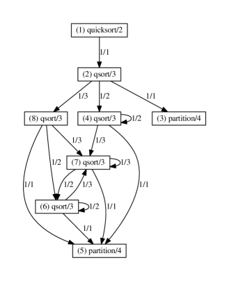
(1)	$\langle quicksort(Xs,Ys),~{}~{}\{Xs/g,Ys/ng\},~{}~{}\{Xs/g,Ys/any\}\rangle$
(2)	$\langle qsort(Xs,Ys,[]),~{}~{}\{Xs/g,Ys/ng\},~{}~{}\{Xs/g,Ys/any\}\rangle$
(3)	$\langle partition(Xs,X,L,R),~{}~{}\{Xs/g,X/g,L/ng,R/ng\}),~{}~{}\{Xs/g,X/g,L/any,R/any\})\rangle$
(4)	$\langle qsort(Xs,Ys,Zs),~{}~{}\{Xs/any,Ys/ng,Zs/g\}),~{}~{}\{Xs/any,Ys/any,Zs/g\})\rangle$
(5)	$\langle partition(Xs,X,L,R),~{}~{}\{Xs/any,X/any,L/ng,R/ng\}),~{}~{}\{Xs/any,X/any,L/any,R/any\})\rangle$
(6)	$\langle qsort(Xs,Ys,Zs),~{}~{}\{Xs/any,Ys/ng,Zs/any\},~{}~{}\{Xs/any,Ys/any,Zs/any\}\rangle$
(7)	$\langle qsort(Xs,Ys,[Z|Zs]),~{}~{}\{Xs/any,Ys/ng,Z/any,Zs/any\}),~{}~{}\{Xs/any,Ys/any,Z/any,Zs/any\})\rangle$
(8)	$\langle qsort(Xs,Ys,[Z|Zs]),~{}~{}\{Xs/any,Ys/ng,Z/g,Zs/any\},~{}~{}\{Xs/any,Ys/any,Z/g,Zs/any\}\rangle$

Figure 7: Analysis of quicksort/2.

quicksort/2/0 (entry)	quicksort/2/1/1	qsort/3/1/1	qsort/3/1/2	qsort/3/1/3
(1)	(2)	(3), (5)	(4), (6)	(7), (8)

The resulting single triples $\langle L,\lambda^{c},\lambda^{s}\rangle$ for each program point will be the following:

quicksort/2/0 (entry)	(1)	$\langle quicksort(Xs,Ys),~{}~{}\{Xs/g,Ys/ng\},~{}~{}\{Xs/g,Ys/any\}\rangle$
quicksort/2/1/1	(2)	$\langle qsort(Xs,Ys,[]),~{}~{}\{Xs/g,Ys/ng\},~{}~{}\{Xs/g,Ys/any\}\rangle$
qsort/3/1/1	(3) ’$\sqcup$’ (5)	$\langle partition(Xs,X,L,R),~{}~{}\{Xs/any,X/any,L/ng,R/ng\}),~{}~{}\{Xs/any,X/any,L/any,R/any\})\rangle$
qsort/3/1/2	(4) ’$\sqcup$’ (6)	$\langle qsort(Xs,Ys,Zs),~{}~{}\{Xs/any,Ys/ng,Zs/any\},~{}~{}\{Xs/any,Ys/any,Zs/any\}\rangle$
qsort/3/1/3	(7) ’$\sqcup$’ (8)	$\langle qsort(Xs,Ys,[Z|Zs]),~{}~{}\{Xs/any,Ys/ng,Z/any,Zs/any\},~{}~{}\{Xs/any,Ys/any,Z/g,Zs/any\}\rangle$

Let us compare the two analyses shown in Figs. 1 and 7. We already have their representation as one triple $\langle L,\lambda^{c},\lambda^{s}\rangle$ for each program point. The distances for each program point, computed as the average of the distance between its abstract call substitution and the distance between its abstract success substitution, is the following:
quicksort/2/0 (entry) quicksort/2/1/1 qsort/3/1/1 qsort/3/1/2 qsort/3/1/3 0.354 0.354 0.427 0.454 0.467

The final distance between the analysis could be the average of all of them, 0.411. Alternatively, we could assign different weights to each program point taking into account the structure of the program, and use a weighted average as final distance. For example, we could assign the weights of the table below, which would yield the final distance 0.378.

quicksort/2/0 (entry)	quicksort/2/1/1	qsort/3/1/1	qsort/3/1/2	qsort/3/1/3
$\frac{1}{2}$	$\frac{1}{4}$	$\frac{1}{12}$	$\frac{1}{12}$	$\frac{1}{12}$

0.B.2 Example of the tree distance

Let us compute the tree distance between the two analyses shown in Figs. 1 and 7. Fig. 8 shows the tree with distances between both analysis node to node. The and-nodes are omitted for simplicity. Each or-node is a quintuple $(P,Id_{1},Id_{2},D,W)$: $P$ is the predicate corresponding to that program point, $I_{1}$ is the identifier of the node in analysis 1 corresponding to that or-node, $I_{2}$ is the analogous in analysis 7, $D$ is the distance between the two nodes, and $W$ is the corresponding weight to the distance in that node when we apply the definition of the tree distance. We use a factor $\mu=\frac{1}{5}$, and the average of the distance between the call substitutions and the distance between the success substitutions as distance between nodes, using an abstract distance in the underlying groundness domain.

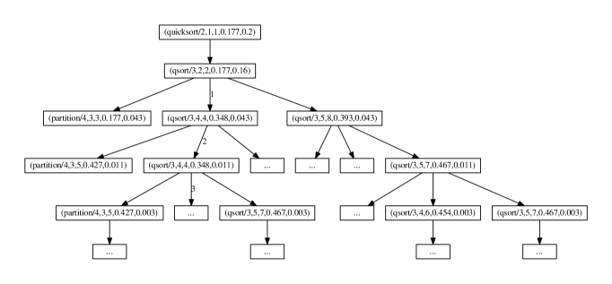
Figure 8: 3rd approach: whole abstract execution tree

If we follow the tree through the edges labelled 1,2,3…, we observe that we are visiting the same node over and over with decreasing weights $0.043,0.011,0.003\ldots=w\frac{1}{5}+w\frac{4}{5}\frac{1}{3}\frac{1}{5}+w\frac{4}{5}\frac{1}{3}\frac{4}{5}\frac{1}{3}\frac{1}{5}+\ldots$, where $w=1\frac{4}{5}\frac{1}{1}\frac{4}{5}\frac{1}{3}$. The sum of those weights converges ($\frac{1}{5}w\sum_{i=0}^{\infty}{(\frac{4}{5}\frac{1}{3})^{i}}=\frac{1}{5}w\frac{15}{11}$), but it is not trivial to compute in the general case and for all cases.

However, we can compute the final sum solving the following systems of equations, where the variable $X_{i,j}$ corresponds to the node $(P,i,j,D,W)$:

$\\ \begin{array}[]{l}\left\{\begin{array}[]{ll}X_{1,1}=\frac{1}{5}*0.177+\frac{4}{5}X_{2,2}\\ X_{2,2}=\frac{1}{5}*0.177+\frac{4}{5}\frac{1}{3}X_{3,3}+\frac{4}{5}\frac{1}{3}X_{4,4}+\frac{4}{5}\frac{1}{3}X_{5,8}\\ X_{3,3}=0.177\\ X_{4,4}=\frac{1}{5}*0.348+\frac{4}{5}\frac{1}{3}X_{3,5}+\frac{4}{5}\frac{1}{3}X_{4,4}+\frac{4}{5}\frac{1}{3}X_{5,7}\\ X_{5,8}=\frac{1}{5}*0.177+\frac{4}{5}\frac{1}{3}X_{3,5}+\frac{4}{5}\frac{1}{3}X_{4,6}+\frac{4}{5}\frac{1}{3}X_{5,7}\\ X_{3,5}=0.427\\ X_{5,7}=\frac{1}{5}*0.177+\frac{4}{5}\frac{1}{3}X_{3,5}+\frac{4}{5}\frac{1}{3}X_{4,6}+\frac{4}{5}\frac{1}{3}X_{5,7}\\ X_{4,6}=\frac{1}{5}*0.177+\frac{4}{5}\frac{1}{3}X_{3,5}+\frac{4}{5}\frac{1}{3}X_{4,6}+\frac{4}{5}\frac{1}{3}X_{5,7}\\ \end{array}\right.\par\end{array}\\$

References

- [1] E. Albert, P. Arenas, S. Genaim, G. Puebla, and D. Zanardini. Cost Analysis of Java Bytecode. In Proc. of ESOP’07, LNCS 4421, pages 157–172. Springer, 2007.
- [2] T. Armstrong, K. Marriott, P. Schachte, and H. Søndergaard. Boolean functions for dependency analysis: Algebraic properties and efficient representation. In Springer-Verlag, editor, Static Analysis Symposium, SAS’94.
- [3] Gourinath Banda and John P. Gallagher. Analysis of Linear Hybrid Systems in CLP. In Michael Hanus, editor, LOPSTR, volume 5438 of LNCS, pages 55–70. Springer, 2009.
- [4] Nikolaj Bjørner, Arie Gurfinkel, Kenneth L. McMillan, and Andrey Rybalchenko. Horn Clause Solvers for Program Verification. In Essays to Yuri Gurevich on his 75th Birthday, pages 24–51, 2015.
- [5] M. Bruynooghe. A Practical Framework for the Abstract Interpretation of Logic Programs. Journal of Logic Programming, 10:91–124, 1991.
- [6] F. Bueno, M. García de la Banda, and M. V. Hermenegildo. Effectiveness of Global Analysis in Strict Independence-Based Automatic Program Parallelization. In International Symposium on Logic Programming, pages 320–336. MIT Press, November 1994.
- [7] A. Cortesi, G. File, and W. Winsborough. Comparison of Abstract Interpretations. In Nineteenth International Colloquium on Automata, Languages, and Programming, volume 623. Springer-Verlag LNCS, 1992.
- [8] P. Cousot and R. Cousot. Abstract Interpretation: a Unified Lattice Model for Static Analysis of Programs by Construction or Approximation of Fixpoints. In Proc. of POPL’77, pages 238–252. ACM Press, 1977.
- [9] P.W. Dart and J. Zobel. A Regular Type Language for Logic Programs. In Types in Logic Programming, pages 157–187. MIT Press, 1992.
- [10] Emanuele De Angelis, Fabio Fioravanti, Alberto Pettorossi, and Maurizio Proietti. VeriMAP: A Tool for Verifying Programs through Transformations. In TACAS, ETAPS, pages 568–574, 2014.
- [11] Luc De Raedt and Jan Ramon. Deriving distance metrics from generality relations. Pattern Recogn. Lett., 30(3):187–191, February 2009.
- [12] S. K. Debray. Static Inference of Modes and Data Dependencies in Logic Programs. ACM Transactions on Programming Languages and Systems, 11(3):418–450, 1989.
- [13] Alessandra Di Pierro and Herbert Wiklicky. Measuring the precision of abstract interpretations. In Logic Based Program Synthesis and Transformation, pages 147–164, Berlin, Heidelberg, 2001. Springer Berlin Heidelberg.
- [14] I. Garcia-Contreras, J. F. Morales, and M. V. Hermenegildo. Semantic Code Browsing. TPLP (ICLP’16 Special Issue), 16(5-6):721–737, October 2016.
- [15] M. García de la Banda and M. V. Hermenegildo. A Practical Application of Sharing and Freeness Inference. In 1992 Workshop on Static Analysis WSA’92, number 81–82 in BIGRE, pages 118–125, Bourdeaux, France, September 1992. IRISA-Beaulieu.
- [16] M. García de la Banda, M. V. Hermenegildo, M. Bruynooghe, V. Dumortier, G. Janssens, and W. Simoens. Global Analysis of Constraint Logic Programs. ACM TOPLAS, 18(5), 1996.
- [17] S. Grebenshchikov, A. Gupta, N. P. Lopes, Co. Popeea, and A. Rybalchenko. HSF(C): A Software Verifier Based on Horn Clauses. In TACAS, pages 549–551, 2012.
- [18] George Grätzer. General Lattice Theory, second edition. 01 1998.
- [19] Arie Gurfinkel, Temesghen Kahsai, Anvesh Komuravelli, and Jorge A. Navas. The SeaHorn Verification Framework. In CAV, pages 343–361, 2015.
- [20] M. Hermenegildo, G. Puebla, F. Bueno, and P. Lopez-Garcia. Integrated Program Debugging, Verification, and Optimization Using Abstract Interpretation (and The Ciao System Preprocessor). Science of Comp. Progr., 58(1–2), 2005.
- [21] M. Hermenegildo, R. Warren, and S. K. Debray. Global Flow Analysis as a Practical Compilation Tool. JLP, 13(4):349–367, August 1992.
- [22] Alan Hutchinson. Metrics on terms and clauses. In Maarten van Someren and Gerhard Widmer, editors, Machine Learning: ECML-97, pages 138–145, Berlin, Heidelberg, 1997. Springer Berlin Heidelberg.
- [23] D. Jacobs and A. Langen. Accurate and Efficient Approximation of Variable Aliasing in Logic Programs. In North American Conference on Logic Programming, 1989.
- [24] B. Kafle, J. P. Gallagher, and J. F. Morales. RAHFT: A Tool for Verifying Horn Clauses Using Abstract Interpretation and Finite Tree Automata. In CAV, pages 261–268, 2016.
- [25] A. Kelly, A. Macdonald, K. Marriott, H. Sondergaard, P. Stuckey, and R. Yap. An optimizing compiler for CLP(R). In Proc. of Constraint Programming (CP’95). LNCS, Springer, 1995.
- [26] U. Liqat, S. Kerrison, A. Serrano, K. Georgiou, P. Lopez-Garcia, N. Grech, M. V. Hermenegildo, and K. Eder. Energy Consumption Analysis of Programs based on XMOS ISA-level Models. In LOPSTR, volume 8901 of LNCS, pages 72–90. Springer, 2014.
- [27] Francesco Logozzo, Corneliu Popeea, and Vincent Laviron. Towards a quantitative estimation of abstract interpretations (extended abstract). In Workshop on Quantitative Analysis of Software, June 2009.
- [28] Magnus Madsen, Ming-Ho Yee, and Ondrej Lhoták. From Datalog to FLIX: a Declarative Language for Fixed Points on Lattices. In PLDI, ACM, pages 194–208, 2016.
- [29] K. Marriott, H. Søndergaard, and N.D. Jones. Denotational Abstract Interpretation of Logic Programs. ACM Transactions on Programming Languages and Systems, 16(3):607–648, 1994.
- [30] K. Muthukumar and M. Hermenegildo. Determination of Variable Dependence Information at Compile-Time Through Abstract Interpretation. In NACLP’89, pages 166–189. MIT Press, October 1989.
- [31] K. Muthukumar and M. Hermenegildo. Combined Determination of Sharing and Freeness of Program Variables Through Abstract Interpretation. In ICLP’91, pages 49–63. MIT Press, June 1991.
- [32] J. Navas, F. Bueno, and M. V. Hermenegildo. Efficient Top-Down Set-Sharing Analysis Using Cliques. In 8th Int’l. Symp. on Practical Aspects of Declarative Languages (PADL’06), number 2819 in LNCS, pages 183–198. Springer, January 2006.
- [33] J. Navas, M. Méndez-Lojo, and M. V. Hermenegildo. User-Definable Resource Usage Bounds Analysis for Java Bytecode. In BYTECODE’09, volume 253 of ENTCS. Elsevier, March 2009.
- [34] Shan-Hwei Nienhuys-Cheng. Distance between herbrand interpretations: A measure for approximations to a target concept. In Nada Lavrač and Sašo Džeroski, editors, Inductive Logic Programming, pages 213–226, Berlin, Heidelberg, 1997. Springer Berlin Heidelberg.
- [35] G. Puebla, F. Bueno, and M. V. Hermenegildo. An Assertion Language for Constraint Logic Programs. In P. Deransart, M. V. Hermenegildo, and J. Maluszynski, editors, Analysis and Visualization Tools for Constraint Programming, number 1870 in LNCS, pages 23–61. Springer-Verlag, September 2000.
- [36] J. Ramon and M. Bruynooghe. A framework for defining distances between first-order logic objects. In 8th Intl. WS on Inductive Logic Programming, pages 271–280, 1998.
- [37] Pascal Sotin. Quantifying the Precision of Numerical Abstract Domains. Research report, INRIA, February 2010.
- [38] P. Van Roy and A.M. Despain. High-Performance Logic Programming with the Aquarius Prolog Compiler. IEEE Computer Magazine, pages 54–68, January 1992.